General mapping of multi-qu$d$it entanglement conditions to non-separability indicators for quantum optical fields

Abstract

We show that any multi-qudit entanglement witness leads to a non-separability indicator for quantum optical fields, which involves intensity correlations. We get, e.g., necessary and sufficient conditions for intensity or intensity-rate correlations to reveal polarization entanglement. We also derive separability conditions for experiments involving multiport interferometers, now feasible with integrated optics. We show advantages of using intensity rates rather than intensities, e.g., a mapping of Bell inequalities to ones for optical fields. The results have implication for studies of non-classicality of “macroscopic” systems of undefined or uncontrollable number of “particles”.

Non-classicality due to entanglement initially was studied using quantum optical multiphoton interferometry, see e.g., PAN . The experiments were constrained to defined photon number states, e.g., the two-photon polarization singlet ASPECT . This includes Greenberger-Horne-Zeilinger (GHZ) GHZ inspired multiphoton interference, with an interpretation that each detection event signals one photon. Spurious events of higher photon number counts contributed to a lower interferometric contrast. Still, states of undefined photon numbers, e.g., the squeezed vacuum, can be entangled BANASZEK ; BOUW ; MASZA-REVIEW .

This form of entanglement of quantum optical fields served e.g., to show that a strongly pumped two-mode (bright) squeezed state allows one to directly refute the ideas of EPR EPR , as it approximates their state, and a form of Bell’s Theorem can be shown for it BANASZEK . The trick was to use displaced parity observables. Recently it has been shown that this is also possible for four-mode bright squeezed vacuum ROSOLEK , which can be produced via type II parametric down-conversion, see e.g BOUW ; MASZA-REVIEW . In this case the state approximates a tensor product of two EPR states, and interestingly can also be thought of as a polarization “super-singlet” of undefined photon numbers DURKIN . The approach of Ref. ROSOLEK used (effectively) intensity observables, which are less experimentally cumbersome.

With the birth of quantum information science and technology, entanglement became a resource. We have an extended literature on detection of entanglement for systems of finite dimensions, essentially “particles”, see e.g., HORODECKIS . It is well known that not all entangled states violate Bell inequalities. Still there is theory of entanglement indicators, called usually witnesses, which allow to detect entanglement, even if a given state for finite dimensional systems (essentially, qu$d$its) does not violate any known Bell inequalities. The case of two-mode entanglement for optical fields was studied in trailblazing papers of SIMON ; DUAN , which discussed “two-party continuous variable systems”, and with a direct quantum optical formalism in HILLERY . The entanglement conditions reached in the papers did not involve intensity correlations.

An entanglement condition for four-mode fields, which was borrowing ideas from two spin-1/2 (two-qubit) correlations, involved correlations Stokes operators and was first discussed in BOUW . The resulting indicator was used to measure efficiency of an “entanglement laser”. The output of the “laser” was bright four-mode vacuum. We shall present here the most extensive generalization of such an approach, i.e., entanglement indicators for optical fields which are derivatives of multi-qudit entanglement witnesses involving intensity correlations. In Supplementary Material supp we give examples of entanglement conditions based on such an approach. Some of them are more tight versions of the entanglement conditions mentioned above.

As a growing part of the experimental effort is now directed at non-classical features of bright (intensive, “macroscopic”) beams of light, e.g., Lamas01 ; BOUW-2 ; Eckstein11 ; Iskhakov12 ; Iskhakov13 ; Kanseri13 ; Spasibko17 so the time is ripe for a comprehensive study of such entanglement conditions. All that may lead to some new schemes in quantum communication and quantum cryptography, perhaps on the lines of Ref. DURKIN . The emergence of integrated optics allows now to construct stable multiport interferometers Mattle95 ; Weihs96 ; Peruzzo11 ; Meany12 ; Metcalf13 ; Spagnolo13 ; Carolan15 ; Schaeff15 , and is our motivation of going beyond two times mode case.

We present a theory of mapping multi-qu$d$it entanglement witnesses HORODECKIS into entanglement indicators for quantum optical fields, which employ intensity correlations or correlations of intensity rates. By intensity rates we mean the ratio of intensity at a given local detector and the sum of intensities at all local detectors (in some case the second approach leads to better entanglement detection). The method may find applications also in studies of non-classicality of correlations in “macroscopic” many-body quantum systems of undefined or uncontrollable number of constituents, e.g., Bose-Einstein condensates SORENSEN , other specific states of cold atoms POLZIK ; sorensenPRL .

The essential ideas are presented for polarization measurements by two observers and the most simple model of intensity observable: photon-number in the observed mode. Next, we present further generalization of our approach, and examples employing specific indicators involving intensity correlations for unbiased multiport interferometers. We discuss generalizations to multi-party entanglement indicators. We show that the use of rates leads to a modification of quantum optical Glauber correlation functions, which gives a new tool for studying non-classicality, and that it also gives a general method of mapping standard Bell inequalities into ones for optical fields.

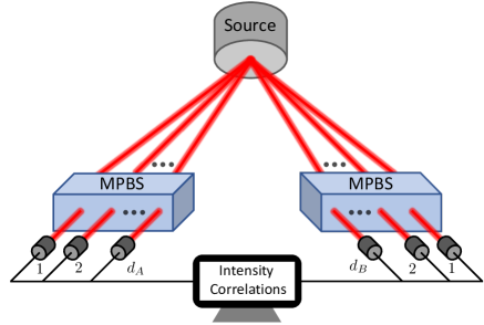
Figure 1: The experiments (two parties). Two multi-mode beams propagate to two spatially separated measurement stations. Each station consists of a $d$ input $d$ output tunable multi-port beamsplitter-interferometer (MPBS) and detectors at its outputs. For polarization measurements put $d_{A}=d_{B}=2$, and treat the paths as polarization modes.

We discuss spatially separated stations, $X=A,B,...$ with (passive) interferometers of $d_{X}$ input and output ports, FIG. 1. In each output there is a detector which measures intensity. One can assume either a pulsed source, sources acting synchronously ZUK-ZEIL-WEIN ; KALTENBAEK or that the measurement is performed within a short time gate. Each time gate, or pulsed emission, is treated as a repetition of the experiment building up averages of observables.

Stokes parameters.—For the description of polarization of light, the standard approach uses Stokes parameters. Using the photon numbers they read $\langle\hat{\Theta}_{j}\rangle=\langle\hat{a}_{j}^{\dagger}\hat{a}_{j}-\hat{a}_{{j}_{\perp}}^{\dagger}\hat{a}_{{j}_{\perp}}\rangle,$ where $j,j_{\perp}$ denote a pair of orthogonal polarizations of one of three mutually unbiased polarization bases $j=1,2,3$, e.g., $\{{H},{V}\},\{{45^{\circ}},{-45^{\circ}}\},\{{R},{L}\}$. The zeroth parameter $\langle\hat{\Theta}_{0}\rangle$ is the total intensity: $\langle\hat{N}\rangle=\langle\hat{a}_{j}^{\dagger}\hat{a}_{j}+\hat{a}_{{j}_{\perp}}^{\dagger}\hat{a}_{{j}_{\perp}}\rangle.$ Alternative normalized Stokes observables were studied by some of us zuko ; zuko1 ; zuko2 . They were first intorduced in HE , however a different technical approach was used. Following zuko one can put $\langle\hat{S}_{j}\rangle=\langle\hat{\Pi}\frac{(\hat{a}_{j}^{\dagger}\hat{a}_{j}-\hat{a}_{{j}_{\perp}}^{\dagger}\hat{a}_{{j}_{\perp}})}{\hat{N}}\hat{\Pi}\rangle,$ and $\langle\hat{S}_{0}\rangle=\langle\hat{\Pi}\rangle$, where $\hat{\Pi}=\mathbb{1}-\outerproduct{\Omega}{\Omega}$ and $|\Omega\rangle$ is the vacuum state for the considered modes, $\hat{a}_{j}|\Omega\rangle=\hat{a}_{j_{\perp}}|\Omega\rangle=0$. Operationally, in the $r$-th run of an experiment, we register photon numbers in the two exits of a polarization analyzer, $n^{r}_{j}$ and $n^{r}_{j_{\perp}}$, and divide their difference by their sum. If $n^{r}_{j}+n^{r}_{j_{\perp}}=0$ , the value is put as zero. This does not require any additional measurements, only the data are differently processed than in the standard approach. In zuko ; zuko1 ; zuko2 examples of two-party entanglement conditions and Bell inequalities using normalized Stokes operators were given. Here we present a general approach.

Map from two-qubit entanglement witnesses to entanglement indicators for fields involving Stokes parameters.—Pauli operators $\vec{\sigma}=(\hat{\sigma}_{1},\hat{\sigma}_{2},\hat{\sigma}_{3})$ and $\hat{\sigma}_{0}=\mathbb{1}$ form a basis in the real space of one-qubit observables. Thus, any two-qubit entanglement witness, $\hat{W}$, has the following expansion: $\hat{W}=\sum_{\mu,\nu}w_{\mu\nu}\hat{\sigma}_{\mu}^{A}\otimes\hat{\sigma}_{\nu}^{B}$, where $\mu,\nu=0,1,2,3$ and $w_{\mu\nu}$ are real coefficients. We have $\langle\hat{W}\rangle_{sep}\geq 0$, where $\langle\cdot\rangle_{sep}$ denotes an average for a separable state. We will show that with each witness $\hat{W}$ one can associate entanglement indicators for polarization measurements involving correlations of Stokes observables for quantum optical fields. The maps are $\hat{\sigma}_{\mu}^{A}\otimes\hat{\sigma}_{\nu}^{B}\to\hat{S}_{\mu}^{A}\hat{S}_{\nu}^{B}$ and $\hat{\sigma}_{\mu}^{A}\otimes\hat{\sigma}_{\nu}^{B}\to\hat{\Theta}_{\mu}^{A}\hat{\Theta}_{\nu}^{B}$, and they link $\hat{W}$ with its quantum optical analogues $\hat{\mathcal{W}}_{S}=\sum_{\mu,\nu}w_{\mu\nu}\hat{S}_{\mu}^{A}\hat{S}_{\nu}^{B},$ and $\hat{\mathcal{W}}_{\Theta}=\sum_{\mu,\nu}w_{\mu\nu}\hat{\Theta}_{\mu}^{A}\hat{\Theta}_{\nu}^{B},$ which fulfill $\langle\hat{\mathcal{W}}_{S}\rangle_{sep}\geq 0$ and $\langle\hat{\mathcal{W}}_{\Theta}\rangle_{sep}\geq 0$. The proof goes as follows.

Normalized Stokes operators case.—It is enough to prove that for any mixed state $\varrho$ one can find a $4\times 4$ density matrix $\mathbf{\mathfrak{\hat{R}}}^{AB}_{\varrho}$ for a pair of qubits, such that:

$$\frac{\langle{\hat{\mathcal{W}}_{S}}\rangle_{\varrho}}{\langle{\hat{\Pi}^{A}\hat{\Pi}^{B}}\rangle_{\varrho}}=\Tr\hat{W}\mathbf{\mathfrak{\hat{R}}}^{AB}_{\varrho}.$$ (1)

First, we show that (1) holds for any pure state $\ket{\psi^{AB}}$.

Let us denote the polarization basis $H$ and $V$ as $\hat{x}_{H}=\hat{x}_{1}$ and $\hat{x}_{V}=\hat{x}_{2}$. Normalized Stokes operators in arbitrary direction can be put as $\vec{m}\cdot\vec{S}^{X}$, where $\vec{m}$ is an arbitrary unit real vector, or in the matrix form $\sum_{kl}\hat{\Pi}^{X}\frac{{{\hat{x}}_{k}^{\dagger}}(\vec{m}\cdot\vec{\sigma})_{kl}{{\hat{x}_{l}}}}{\hat{N}^{X}}\hat{\Pi}^{X},$ with $\hat{x}=\hat{a}$ or $\hat{b}$ depending on the beam $X$, whereas $\hat{S}_{0}^{X}$ reads $\sum_{kl}\hat{\Pi}^{X}\frac{{{\hat{x}}_{k}^{\dagger}}\delta_{kl}{{\hat{x}_{l}}}}{\hat{N}^{X}}\hat{\Pi}^{X}.$ We introduce a set of states

$$\ket{\mathbf{\Psi}_{km}^{AB}}=\hat{a}_{k}\hat{b}_{m}\frac{1}{\sqrt{\hat{N}^{A}\hat{N}^{B}}}\hat{\Pi}^{A}\hat{\Pi}^{B}\ket{\psi^{AB}},$$ (2)

where $k,m\in\{1,2\}$. This allows us to put

$$\expectationvalue{\hat{S}_{\mu}^{A}\hat{S}_{\nu}^{B}}{\psi^{AB}} = \sum_{k,l=1}^{2}\sum_{m,n=1}^{2}\sigma^{kl}_{\mu}\sigma^{mn}_{\nu}\bra{\mathbf{\Psi}^{AB}_{km}}\ket{\mathbf{\Psi}^{AB}_{ln}}$$ (3)

$$= \Tr\hat{\sigma}_{{\mu}}^{A}\otimes\hat{\sigma}_{{\nu}}^{B}\hat{R}^{AB}_{\psi},$$

where the matrix elements of $\hat{R}^{AB}_{\psi}$ are $\bra{\mathbf{\Psi}^{AB}_{km}}\ket{\mathbf{\Psi}^{AB}_{ln}}$. As a Gramian matrix, ${\hat{R}}^{AB}_{\psi}$ is positive. Except for $|\psi^{AB}\rangle$ describing vacuum at one or both sides, we have $0<\Tr\hat{R}^{AB}_{\psi}=\langle\hat{\Pi}^{A}\hat{\Pi}^{B}\rangle\leq 1$. Thus, $\mathbf{\mathfrak{\hat{R}}}^{AB}_{\psi}=\hat{R}^{AB}_{\psi}/\langle\hat{\Pi}^{A}\hat{\Pi}^{B}\rangle$ is an admissible density matrix of two qubits.

For mixed states $\varrho$, i.e., convex combinations of $\ket{\psi^{AB}_{\lambda}}$’s with weights $p_{\lambda}$, one gets $\hat{R}^{AB}_{\varrho}=\sum_{\lambda}p_{\lambda}{\hat{R}}^{AB}_{\lambda}$ which is positive definite, and its trace is $\sum_{\lambda}p_{\lambda}\Tr\hat{R}^{AB}_{\lambda}\leq 1$. Thus after the re-normalization one gets a proper two-qubit density matrix $\mathbf{\mathfrak{\hat{R}}}^{AB}_{\varrho}$. As purity of a field state $\ket{\psi^{AB}_{\lambda}}$ does not warrant that the corresponding $\hat{R}^{AB}_{\lambda}$ is a projector, $\mathbf{\mathfrak{\hat{R}}}^{AB}_{\varrho}$ does not have to have the same convex expansion coefficients in terms of pure two-qubit states, as $\varrho$ in terms of $\ket{\psi^{AB}_{\lambda}}$’s.

For any separable pure state of two optical beams $|\psi^{AB}\rangle_{prod}$, defined as $F^{\dagger}_{A}F^{\dagger}_{B}|\Omega\rangle$, where $F^{\dagger}_{X}$ is a polynomial function of creation operators for beam (modes) $X$, and $|\Omega\rangle$ is the vacuum state of both beams, the matrix $\hat{R}^{AB}$ factorizes: $\hat{R}^{AB}=\hat{R}^{A}\hat{R}^{B}$. Simply, ${}_{prod}\bra{\mathbf{\Psi}^{AB}_{km}}\ket{\mathbf{\Psi}^{AB}_{ln}}_{prod}$ factorizes to $\bra{\mathbf{\Psi}^{A}_{k}}\ket{\mathbf{\Psi}^{A}_{l}}\bra{\mathbf{\Psi}^{B}_{m}}\ket{\mathbf{\Psi}^{B}_{n}},$ where $\bra{\mathbf{\Psi}^{X}_{k}}\ket{\mathbf{\Psi}^{X}_{l}}$ are elements of matrix $\hat{R}^{X}$ and $|\mathbf{\Psi}_{l}^{X}\rangle=\hat{x}_{l}\frac{1}{\sqrt{\hat{N}^{X}}}\hat{\Pi}^{X}F^{\dagger}_{X}|\Omega\rangle.$ As $\langle\Omega|F_{X}\hat{\Pi}^{X}F^{\dagger}_{X}|\Omega\rangle^{-1}\hat{R}^{X}$ can be shown to be a qubit density matrix and $\langle\hat{W}\rangle_{sep}\geq 0$, therefore for pure separable states of the optical beams $\langle\hat{\mathcal{W}}_{S}\rangle_{prod}\geq 0$. Obviously, $\langle\mathcal{\hat{W}}_{S}\rangle_{sep}\geq 0$ also for all mixed separable states.

Standard Stokes operators case.— Any standard Stokes operator can be put as $\vec{m}\cdot\vec{\Theta}^{X}=\sum_{kl}\hat{x}_{k}^{\dagger}(\vec{m}\cdot\vec{\sigma})_{kl}\hat{x}_{l}.$ We introduce state vectors $\ket{\mathbf{\Phi}_{jk}^{AB}}=\hat{a}_{j}\hat{b}_{k}\ket{\psi^{AB}}$. One has

$$\expectationvalue{\hat{\Theta}_{\mu}^{A}\hat{\Theta}_{\nu}^{B}}{\psi^{AB}}=\Tr\hat{\sigma}^{A}_{\mu}\hat{\sigma}^{B}_{\nu}\hat{P}^{AB},$$ (4)

where the matrix $\hat{P}^{AB}$ has entries $\bra{\mathbf{\Phi}_{km}^{AB}}\ket{\mathbf{\Phi}_{ln}^{AB}}$, it is positive definite, and its trace is $\langle\hat{N}_{A}\hat{N}_{B}\rangle.$ Thus, $\mathbf{\mathfrak{\hat{P}}}^{AB}=\hat{P}^{AB}/\langle\hat{N}^{A}\hat{N}^{B}\rangle$ is an admissible two-qubit density matrix, and one has $\langle\hat{\mathcal{W}}_{\Theta}\rangle_{\varrho}/\langle\hat{N}^{A}\hat{N}^{B}\rangle_{\varrho}=\Tr\hat{W}\mathbf{\mathfrak{\hat{P}}}^{AB}_{\varrho}.$ All that leads to $\langle\hat{\mathcal{W}}_{\Theta}\rangle_{sep}\geq 0$. Note that, for a general state $\mathbf{\mathfrak{\hat{R}}}^{AB}_{\varrho}$ does not have to be equal to $\mathbf{\mathfrak{\hat{P}}}^{AB}_{\varrho}$. Still, $\mathbf{\mathfrak{\hat{R}}}^{AB}=\mathbf{\mathfrak{\hat{P}}}^{AB}$ for states of defined photon numbers in both beams.

Reverse map.— Any linear separability condition expressible in terms of correlation functions of normalized Stokes Parameters reads: $\sum_{\mu\nu}\omega_{\mu\nu}\langle\hat{S}^{A}_{\mu}\hat{S}^{B}_{\nu}\rangle_{sep}\geq 0.$ As two-photon states, with one at A and the other at B, are possible field states, thus for any separable such state we must have $\sum_{\mu\nu}\omega_{\mu\nu}\langle\hat{S}^{A}_{\mu}\hat{S}^{B}_{\nu}\rangle_{sep-2-ph}\geq 0.$ This is algebraically equivalent to $\sum_{\mu\nu}\omega_{\mu\nu}\langle\hat{\sigma}_{\mu}\otimes\hat{\sigma}_{\nu}\rangle_{sep}\geq 0,$ for any two-qubit state. We get an entanglement witness. Therefore, we have an isomorphism. Similar proof applies to standard Stokes observables.

Examples.—In the Supplemental Material supp , we show some examples of entanglement indicators which can be derived with the above method. This includes a necessary and sufficient conditions for detection of entanglement of two optical beams with correlations of Stokes parameters of the two considered kinds.

Detection losses.— Consider the usual model of losses: a perfect detector in front of which is a beamsplitter of transmission amplitude ${\eta}$, with the reflection channel describing the losses. Then, $\langle\hat{\Theta}_{\mu}^{A}\hat{\Theta}_{\nu}^{B}\rangle$ scales down as $\eta^{A}\eta^{B}$ (see Sec. II in the Supplemental Material supp ), where $\eta^{X}$ for $X=A,B$ is the local detection efficiency. We have a full resistance of entanglement detection, using any $\hat{\mathcal{W}}_{\Theta}$, with respect to such losses. A different character of losses may lead to threshold efficiencies.

For the normalized Stokes parameters, it is enough to consider only pure states, because mixed ones, as convex combinations of such, cannot introduce anything new in entanglement conditions linear with respect to the density matrix. Any pure state is a superposition of Fock states $|F\rangle=|n_{i}^{A},n_{i_{\perp}}^{A},n_{j}^{B},n_{j_{\perp}}^{B}\rangle$, where $n_{i}^{X}$ denotes the number of $i$ polarized photons in beam $X$, and $\hat{S}_{\mu}^{A}\hat{S}_{\nu}^{B}$ are diagonal with respect to the Fock basis related with them. Thus, the dependence on efficiencies of the value of an entanglement indicator, in the case of a pure state, depends on the behavior of its Fock components. One can show, see Sec. II in the Supplemental Material supp , that ${\langle F_{\eta}|\hat{S}_{\mu}^{A}\hat{S}_{\nu}^{B}|F_{\eta}\rangle}=H_{F}{\langle F|\hat{S}_{\mu}^{A}\hat{S}_{\nu}^{B}|F\rangle},$ where $|F_{\eta}\rangle$ is the state $|F\rangle$ after the above described losses in both channels, and $H_{F}=\langle F_{\eta}|\hat{S}_{0}^{A}\hat{S}_{0}^{B}|F_{\eta}\rangle$, which reads $\prod_{X=A,B}[1-(1-\eta^{X})^{m^{X}}]$, where $m^{X}$ is the total number of photons in channel $X$, before the losses. Expanding $|F\rangle$ in terms of Fock states with respect to different polarizations than $i,i_{\perp}$ and $j,j_{\perp}$, does not change the values of $m^{X}$, and thus the formula stays put for any indices. Again we have a strong resistance of the entanglement indicators with respect to losses. Especially for states with high photon numbers, the entanglement conditions based on normalized Stokes parameters, may be more resistant to losses, because $0<\eta<1$ one has $\eta<1-(1-\eta)^{n}$.

Multi-party case.— Consider three parties, and the case of indicators of genuine three-beam entanglement. Any genuine three-qubit entanglement witness $\hat{W}^{(3)}$ has the property that it is positive for pure product three-qubit states $|\xi\rangle_{AB,C}=|\psi\rangle_{AB}|\phi\rangle_{C}$, for similar ones with qubits permuted, and for all convex combinations of such states. With any pure partial product state of the optical beams, e.g. $|\Xi\rangle_{AB,C}=F^{\dagger}_{AB}F^{\dagger}_{C}|\Omega\rangle$, where $F^{\dagger}_{AB}$ is an operator built of creation operators for beams $A$ and $B$, etc., one can associate, in a similar way as above, a partially factorizable three-qubit density matrix $\mathfrak{\hat{R}}^{AB}_{\psi}\mathfrak{\hat{R}}^{C}_{\phi}$. Thus, the homomorphism works. Generalizations are obvious.

General Theory.—Consider a beam of $d_{A}$ quantum optical modes propagating toward a measuring station $A$, and a beam of $d_{B}$ modes toward station $B$. We associate with the situation a $d_{A}\times d_{B}$ dimensional Hilbert Space, $\mathbb{C}^{d_{A}}\otimes\mathbb{C}^{d_{B}}$, which contains pure states of a pair of qudits of dimensions $d_{A}$ and $d_{B}$. For $X=A,B$, let $\hat{V}_{i}^{X}$, with $i=1,...,d_{X}^{2}$, be an orthonormal, i.e. $\Tr\hat{V}_{i}^{X}\hat{V}_{j}^{X}=\delta_{ij}$, Hermitian basis of the space of Hermitian operators acting on $\mathbb{C}^{d_{X}}$. Therefore, products $\hat{V}_{i}^{A}\otimes\hat{V}_{j}^{B}$ form an orthonormal basis of the space of Hermitian operators acting on $\mathbb{C}^{d_{A}}\otimes\mathbb{C}^{d_{B}}$. Thus, any entanglement witness for the pair of qudits, $\hat{W}$, can be expanded into

$$\hat{W}=\sum_{j=1}^{d_{A}^{2}}\sum_{k=1}^{d_{B}^{2}}w_{jk}\hat{V}_{j}^{A}\otimes\hat{V}_{k}^{B},$$ (5)

with real $w_{jk}$. The optimal expansion (with the minimal number of terms) is to use a Schmidt basis for $\hat{W}$.

Each $\hat{V}^{X}_{j}$ can be decomposed to a linear combination of its spectral projections linked with their respective eigenbases, $|x^{(j)}_{l}\rangle$, where $x=a$ or $b$ consistently with $X$ and $l=1,...,d_{X}$. If one fixes a certain pair of bases in $\mathbb{C}^{d_{A}}$ and $\mathbb{C}^{d_{B}}$ as “computational ones”, i.e., starting ones, denoted as $|l_{x}\rangle$, one can always find local unitary matrices $U^{X}(j)$ such that $U^{X}(j)|l_{x}\rangle=|x^{(j)}_{l}\rangle$. The construction of Reck et al. RECK fixes (phases in) a local multiport interferometer, which performs such a transformation. We shall call such interferometers $U^{X}(j)$ ones. In the case of field modes a passive interferometer performs the following mode transformation: $\sum_{k}U^{X}(j)_{lk}\hat{x}^{\dagger}_{k}=\hat{x}^{\dagger}_{l}(j)$, where $\hat{x}^{\dagger}_{l}(j)$ is the photon creation operator in the $l$-th exit mode of interferometer $U^{X}(j)$.

A two-party entanglement witness $\hat{\mathcal{W}}_{R}$ for optical fields, which uses correlations of intensity rates behind pairs of $U^{X}(j)$ interferometers can be constructed as follows. For the output $l_{x}$ of an interferometer, one defines rate observables as $\hat{r}_{l_{x}}=\hat{\Pi}^{X}\frac{\hat{n}_{l_{x}}}{\hat{N}^{X}}\hat{\Pi}^{X}$, where $\hat{N}^{X}=\sum_{l_{x}=1}^{d_{X}}\hat{n}_{l_{x}}$. The witness $\hat{W}$ expanded in terms of the computational basis:

$$\hat{W}=\sum_{k,m}^{{d}_{A}}\sum_{l,n}^{{d}_{B}}w_{klmn}|k_{a},l_{b}\rangle\langle m_{a},n_{b}|,$$ (6)

allows us to form an entanglement witness for fields:

$$\hat{\mathcal{W}}_{R}=\sum_{k,m}\sum_{l,n}w_{klmn}\hat{\Pi}^{A}\hat{\Pi}^{B}\frac{\hat{a}^{\dagger}_{k}\hat{b}^{\dagger}_{l}\hat{a}_{m}\hat{b}_{n}}{\hat{N}^{A}\hat{N}^{B}}\hat{\Pi}^{A}\hat{\Pi}^{B}.$$ (7)

For any pure state of the quantum beams $|\Psi\rangle$

$$\frac{\langle\Psi|\hat{\mathcal{W}}_{R}|\Psi\rangle}{\langle\Psi|\hat{\Pi}^{A}\hat{\Pi}^{B}|\Psi\rangle}=\Tr\hat{W}\hat{\mathcal{R}},$$ (8)

where the matrix $\hat{\mathcal{R}}$ has elements $r_{klmn}$

$$r_{klmn}=\frac{1}{\langle\Psi|\hat{\Pi}^{A}\hat{\Pi}^{B}|\Psi\rangle}\langle\Psi|\hat{\Pi}^{A}\hat{\Pi}^{B}\frac{\hat{a}^{\dagger}_{k}\hat{b}^{\dagger}_{l}\hat{a}_{m}\hat{b}_{n}}{\hat{N}^{A}\hat{N}^{B}}\hat{\Pi}^{A}\hat{\Pi}^{B}|\Psi\rangle.$$ (9)

Using a generalization of the earlier derivations one can show that $\hat{\mathcal{R}}$ is a two-qudit density matrix, and so on.

The actual measurements, to be correlations of local ones, should be performed using the sequence of pairs of $U^{X}(j)$ interferometers, which enter the expansion of the two-qudit entanglement witness (5). In the entanglement indicator the rates at output $x_{l}(j)$ of the given local interferometer $U^{X}(j)$ are multiplied by the respective eigenvalue of $\hat{V}_{j}^{X}$ related with the eigenstate $|x^{(j)}_{l}\rangle$.

To get an entanglement witness for intensities $\mathcal{\hat{W}}_{I}$ we take $\hat{W}$ and replace the computational basis kets and bras by suitable creation and annihilation operators:

$$\hat{\mathcal{W}}_{I}=\sum_{k,m}^{{d}_{A}}\sum_{l,n}^{{d}_{B}}w_{klmn}\hat{a}^{\dagger}_{k}\hat{b}^{\dagger}_{l}\hat{a}_{m}\hat{b}_{n}.$$ (10)

For any pure state of the quantum beams $|\Psi\rangle$ one has $\frac{\langle\Psi|\hat{\mathcal{W}}_{I}|\Psi\rangle}{\langle\Psi|\hat{N}_{A}\hat{N}_{B}|\Psi\rangle}=\Tr\hat{W}{\hat{\mathcal{P}}},$ where the matrix $\hat{\mathcal{P}}$ has elements $\frac{1}{\langle\Psi|\hat{N}_{A}\hat{N}_{B}|\Psi\rangle}\langle\Psi|\hat{a}^{\dagger}_{k}\hat{b}^{\dagger}_{l}\hat{a}_{m}\hat{b}_{n}|\Psi\rangle,$ and has all properties of a two-qudit density matrix.

Example showing further extension to unitary operator bases.—Let $d$ be a power of a prime number. Consider $d_{A}=d_{B}=d$ beams experiment (see Fig. 1), with families of $U^{X}(m)$ interferometers which link the computational basis of a qudit with an unbiased basis $m$, belonging to the full set of $d+1$ mutually unbiased ones WOOTERS ; MUBs . We introduce a set of unitary observables for a qudit: $\hat{q}_{k}(m)=\sum_{j=1}^{d}\omega^{jk}|j(m)\rangle\langle j(m)|,$ with $|j(m)\rangle=U(m)|j\rangle$ and it is the $j$-th member of $m$-th mutually unbiased basis, and $\omega=\exp(2\pi i/d)$. Operators $\hat{q}_{k}(m)/\sqrt{d}$ with $k=1,...,d-1$ and $m=0,...,d$ and $\hat{q}_{0}(0)/\sqrt{d}$ form an orthonormal basis in the Hilbert-Schmidt space of all $d\times d$ matrices (see Sec. III in the Supplemental Material supp ). Thus, we can expand any qudit density matrix as

$${\varrho}=\frac{1}{\sqrt{d}}\left[c_{0,0}\hat{q}_{0}(0)+\sum_{m=0}^{d}\sum_{k=1}^{d-1}c_{m,k}\hat{q}_{k}(m)\right],$$ (11)

where $c_{m,k}=\Tr\hat{q}_{k}^{\dagger}(m)\varrho/\sqrt{d},$ and $c_{0,0}=1/\sqrt{d}$. As the basis observables are unitary the expansion coefficients of an entanglement witness operator in terms of such tensor products of such bases are in general complex. This is no problem for theory, but renders useless a direct application in experiments, as one cannot expect the experimental averages to be real, and thus one has to introduce modifications. Below we present one.

The condition $\Tr\varrho^{2}\leq 1$ can be put as

$$\frac{1}{d}+\frac{1}{d}\sum_{m=0}^{d}\sum_{k=1}^{d-1}\left|\Tr\varrho\hat{q}_{k}(m)\right|^{2}\leq 1.$$ (12)

Thus, applying Cauchy-Schwartz estimate, we get immediately a separability condition for two qudits:

$$\sum_{m=0}^{d}\sum_{k=1}^{d-1}\left|\Tr\varrho^{AB}_{sep}\hat{q}^{A}_{k}(m)\hat{q}^{B\dagger}_{k}(m)\right|\leq(d-1).$$ (13)

Our general method defines a Cauchy-Schwartz-like separability condition homomorphic with (13) as

$$\sum_{m=0}^{d}\sum_{k=1}^{d-1}|\langle\hat{Q}_{k}^{A}(m)\hat{Q}_{k}^{B{\dagger}}(m)\rangle_{sep}|\leq(d-1)\langle\hat{\Pi}^{A}\hat{\Pi}^{B}\rangle_{sep},$$ (14)

where

$$\hat{Q}_{k}^{X}(m)=\sum_{j=1}^{d}\hat{\Pi}^{X}\frac{\omega^{jk}\hat{n}^{X}_{j}(m)}{\hat{N}^{X}}\hat{\Pi}^{X}.$$ (15)

Here $\hat{n}^{X}_{j}(m)=\hat{x}^{\dagger}_{j}(m)\hat{x}_{j}(m)$ is a photon number operator for output mode $j$ of a multiport $m$, at station $X$. For generalized observables based on intensity, one can introduce ${\hat{\chi}}_{k}(m)=\sum_{j=1}^{d}\omega^{jk}\hat{n}_{j}(m)$ to get the following separability condition:

$$\sum_{m=0}^{d}\sum_{k=1}^{d-1}|\langle{\hat{\chi}}_{k}^{A}(m){\hat{\chi}}_{k}^{B{\dagger}}(m)\rangle_{sep}|\leq(d-1)\langle\hat{N}^{A}\hat{N}^{B}\rangle_{sep}.$$ (16)

Supplemental Material presents other examples supp .

Implications for optical coherence theory.—The approach can be generalized further. Let us take as an example Glauber’s correlation functions for optical fields, say $G^{(4)}$ in the form of $\langle\hat{I}_{A}(\vec{x},t)\hat{I}_{B}(\vec{x}^{\prime},t^{\prime})\rangle$, where the intensity operator has the usual form of $I_{X}(\vec{x},t)=\hat{F}_{X}^{\dagger}(\vec{x},t)\hat{F}_{X}(\vec{x},t)$, with normal ordering requiring that operator $\hat{F}_{X}(\vec{x},t)$ is built out of local annihilation operators. The idea of normalized Stokes operators suggests the following alternative correlation function $\Gamma^{4}(\vec{x},t;\vec{x}^{\prime},t^{\prime})$ given by

$$\langle\Pi^{A}\Pi^{B}\frac{\hat{I}_{A}(\vec{x},t)\hat{I}_{B}(\vec{x}^{\prime},t^{\prime})}{\int_{a(A)}d\sigma(\vec{x})\hat{I}_{A}(\vec{x},t)\int_{a(B)}d\sigma(\vec{x}^{\prime})\hat{I}_{B}(\vec{x}^{\prime},t^{\prime})}\Pi^{A}\Pi^{B}\rangle,$$

where $a(X)$ denotes the overall aperture of the detectors in location $X$. Obviously one has $\int_{a(A)}d\sigma(\vec{x})\int_{a(B)}d\sigma(\vec{x}^{\prime})\Gamma^{4}(\vec{x},t;\vec{x}^{\prime},t^{\prime})=\langle\Pi^{A}\Pi^{B}\rangle$, and for fixed $t$ and $t^{\prime}$ one can define

$$\varrho(\vec{x},\vec{y},\vec{x}^{\prime}\vec{y}^{\prime})_{t,t^{\prime}}={\langle\Pi^{A}\Pi^{B}\rangle}^{-1}$$

$$\times\langle\Pi^{A}\Pi^{B}\frac{\hat{F}^{\dagger}_{A}(\vec{y},t)\hat{F}_{A}(\vec{x},t)\hat{F}^{\dagger}_{B}(\vec{y}^{\prime},t^{\prime})\hat{F}_{B}(\vec{x}^{\prime},t^{\prime})}{\int_{a(A)}d\sigma(\vec{x})\hat{I}_{A}(\vec{x},t)\int_{a(B)}d\sigma(\vec{x}^{\prime})\hat{I}_{B}(\vec{x}^{\prime},t^{\prime})}\Pi^{A}\Pi^{B}\rangle,$$

which behaves like a proper two-particle density matrix, provided one constrains the range of $\vec{x},\vec{y},\vec{x}^{\prime},\vec{y}^{\prime}$ to appropriate sets of apertures. As our earlier considerations use simplified forms of (General mapping of multi-qu$d$it entanglement conditions to non-separability indicators for quantum optical fields), it is evident that such correlation functions may help us to unveil non-classicality in situations in which the standard ones fail, see e.g. ROSOLEK .

Bell inequalities.—The above ideas allow one to introduce a general mapping of qudit Bell inequalities to the ones for optical fields. A two-qudit Bell inequality for a final number of local measurement settings $\alpha$ and $\beta$ has the following form:

$$\sum_{\alpha\beta}\sum_{i=1}^{d_{A}}\sum_{j=1}^{d_{B}}K^{ij}_{\alpha\beta}P_{ij}(\alpha,\beta)$$

$$+\sum_{i=1}^{d_{A}}\sum_{\alpha}N^{i}_{\alpha}P_{i}(\alpha)+\sum_{j=1}^{d_{B}}\sum_{\beta}M^{j}_{\beta}P_{j}(\beta)\leq L_{R},$$ (18)

where $P_{ij}(\alpha,\beta)$ denotes the probability of the qudits ending up respectively at detectors $i$ and $j$, when the local setting are as indicated, and $\sum_{j}P_{ij}(\alpha,\beta)=P_{i}(\alpha)$ and $P_{j}(\beta)=\sum_{i}P_{ij}(\alpha,\beta)$. The coefficient matrices $K,N,M$ are real, and $L_{R}$ is the maximum value allowed by local realism. The bound is calculated by putting $P_{ij}(\alpha,\beta)=D^{i}(\alpha)D^{j}(\beta)$ and $P_{i}(\alpha)=D^{i}(\alpha)$, $P_{j}(\beta)=D^{j}(\beta)$, with constraints $0\leq D^{i}(\alpha/\beta)\leq 1$, and $\sum_{i=1}^{d_{A/B}}D^{i}(\alpha/\beta)=1$. As for a given run of a quantum optical experiment local measured photon intensity rates $r_{i}(\alpha)$ and $r_{j}(\beta)$ satisfy exactly the same constraints. We can replace $P_{ij}(\alpha,\beta)\rightarrow\langle r_{i}(\alpha)r_{j}(\beta)\rangle_{LR}$, and $P_{i}(\alpha)\rightarrow\langle r_{i}(\alpha)\rangle_{LR}$, etc., where $\langle.\rangle_{LR}$ is an average in the case of local realism. The bound $L_{R}$ stays put. To get a Bell operator we further replace the above by rate observables $\hat{r}_{i}(\alpha)\hat{r}_{j}(\beta)$, etc. Thus any (multiparty) Bell inequality, see e.g. BELL-RMP , can be useful in quantum optical intensity (rates) correlation experiments. The presented methods for entanglement indicators and Bell inequalities allow also to get steering inequalities for quantum optics.

Conclusions.—We present tools for a construction of entanglement indicators for optical fields, inspired by the vast literature HORODECKIS on entanglement witnesses for finite dimensional quantum systems. The indicators would be handy for more intense light beams in states of undefined photon numbers, especially in the emerging field of integrated optics multi-spatial mode interferometry (see Supplemental Material supp for examples). One may expect applications in the case of many-body systems, e.g. for an analysis of non-classicality of correlations in Bose-Einstein condensates, like in the ones reported in SCHMIED .

Supplemental material

We give here several examples, and more details concerning some derivations. All separability conditions are generalizations or tighter versions of conditions presented in BOUW-2 ; BOUW ; zuko ; MULTIPORT ; MULTIPORT2 , which were derived using various less general approaches.

I Necessary and Sufficient conditions for intensity and rate correlations to reveal entanglement

Two-qubit states are separable if and only if their partial transposes are positive. Yu et al. derived an equivalent family of conditions for two-qubit states CHINY in a form of an inequality, which reads

$$\langle\hat{\sigma}_{1}^{A}\hat{\sigma}_{1}^{B}+\hat{\sigma}_{2}^{A}\hat{\sigma}_{2}^{B}\rangle^{2} + \langle\hat{\sigma}_{3}^{A}\hat{\sigma}_{0}^{{B}}+\hat{\sigma}_{0}^{{A}}\hat{\sigma}_{3}^{B}\rangle^{2}$$ (19)

$$\leq \langle\hat{\sigma}_{0}^{A}\hat{\sigma}_{0}^{B}+\hat{\sigma}_{3}^{A}\hat{\sigma}_{3}^{B}\rangle^{2},$$

where $\hat{\sigma}^{X}_{j}=\vec{n}^{X}_{j}\cdot\vec{\sigma}^{X}$ for $X=A,B$, and the unit vectors $\vec{n}^{X}_{j}$ form a right-handed Cartesian basis triad. If a two-qubit state is entangled, then there exists at least one pair of such triads for which the inequality is violated. The conditions can be put in a form of a family of entanglement witnesses:

$$W(\alpha)=\hat{\sigma}_{0}^{A}\hat{\sigma}_{0}^{B}+\hat{\sigma}_{3}^{A}\hat{\sigma}_{3}^{B} + \sin{\alpha}(\hat{\sigma}_{1}^{A}\hat{\sigma}_{1}^{B}+\hat{\sigma}_{2}^{A}\hat{\sigma}_{2}^{B})$$ (20)

$$+ \cos{\alpha}(\hat{\sigma}_{3}^{A}\hat{\sigma}_{0}^{{B}}+\hat{\sigma}_{0}^{{A}}\hat{\sigma}_{3}^{B}).$$

Our homomorphisms can be used to get the following zuko1 : for normalized Stokes operators

$$\langle\hat{S}_{1}^{A}\hat{S}_{1}^{B}+\hat{S}_{2}^{A}\hat{S}_{2}^{B}\rangle^{2} + \langle\hat{S}_{3}^{A}\hat{\Pi}^{{B}}+\hat{\Pi}^{{A}}\hat{S}_{3}^{B}\rangle^{2}$$ (21)

$$\leq \langle\hat{\Pi}^{A}\hat{\Pi}^{B}+\hat{S}_{3}^{A}\hat{S}_{3}^{B}\rangle^{2},$$

and for standard ones

$$\langle\hat{\Theta}_{1}^{A}\hat{\Theta}_{1}^{B}+\hat{\Theta}_{2}^{A}\hat{\Theta}_{2}^{B}\rangle^{2} + \langle\hat{\Theta}_{3}^{A}\hat{N}^{{B}}+\hat{N}^{{A}}\hat{\Theta}_{3}^{B}\rangle^{2}$$ (22)

$$\leq \langle\hat{N}^{A}\hat{N}^{B}+\hat{\Theta}_{3}^{A}\hat{\Theta}_{3}^{B}\rangle^{2}.$$

The homomorphisms warrant that the violations of conditions (21) and (22) are necessary and sufficient to detect entanglement via measurements of correlations of the Stokes observables. That is, any other condition is sub-optimal, including the ones presented in BOUW , Iskhakov12 and BOUW-2 for standard Stokes observables.

From the necessary and sufficient condition (21) one can derive its corollary, which is a necessary condition for separability:

$$\sum_{j=1}^{3}|\langle{\hat{S}}_{{j}}^{A}{\hat{S}}_{{j}}^{B}\rangle_{sep}|\leq\langle\hat{\Pi}^{A}\hat{\Pi}^{B}\rangle_{sep}.$$ (23)

The condition can be thought as a more tight refinement of the result in BOUW-2 . It can be derived using the fact that for two qubits any of the observables $\sum_{k}s_{k}\sigma^{A}_{k}\sigma^{B}_{k}+\sigma^{A}_{0}\sigma^{B}_{0}$, for arbitrary $s_{k}=\pm 1$ is non-negative for separable states. This can be reached via an application of the Cauchy inequality for a product pure states of a pair of qubits. Next we apply the homomorphism. One can also see that (23) is the separability condition (14) in the main text for $d=2$.

For the standard Stokes operators the associated separability condition (23) reads

$$\sum_{j=1}^{3}|\langle\hat{\Theta}_{j}^{A}\hat{\Theta}_{j}^{B}\rangle_{sep}|\leq\langle{\hat{N}}^{A}{\hat{N}}^{B}\rangle_{sep}.$$ (24)

This is a tighter version of the condition given in BOUW-2 .

For states, which locally lead to vanishing averages of local Stokes parameters, here $\langle\hat{S}^{A}_{i}\hat{\Pi}^{B}\rangle=0$, etc., (e.g., for an ideal four-mode bright squeezed vacuum, see below), the conditions (23) and (21) are equivalent. Thus, in such a case the Cauchy inequality based condition is necessary and sufficient for detection of entanglement with normalized Stokes operators. A similar statement can be produced for the analog condition involving traditional Stokes parameters $\Theta_{j}$, given by (24).

Cauchy-like inequality condition vs. EPR inspired approach.—Consider four-mode (bright) squeezed vacuum represented by

$$\ket{\Psi^{-}}=\frac{1}{\cosh^{2}\Gamma}\sum_{n=0}^{\infty}\sqrt{n+1}\tanh^{n}\Gamma{\color[rgb]{0,0,0}\ket{\psi^{n}_{-}}},$$ (25)

where $\Gamma$ describes a gain which is proportional to the pump power, and $\ket{\psi^{n}_{-}}$ reads

$$\ket{\psi^{n}_{-}}=\frac{1}{n!\sqrt{n+1}}\bigg{(}\hat{a}_{i}^{\dagger}\hat{b}_{i_{\perp}}^{\dagger}-\hat{a}_{i_{\perp}}^{\dagger}b_{i}^{\dagger}\bigg{)}^{n}\ket{\Omega},$$ (26)

where $\ket{\Omega}$ is the vacuum state.

Perfect EPR-type anti-correlations of which are the main trait of the state allow one to formulate the following appealing separability condition (Simon and Bouwmeester, BOUW ):

$$\sum_{j=1}^{3}\langle(\hat{\Theta}_{j}^{A}+\hat{\Theta}_{j}^{B})^{2}\rangle_{sep}\geq 2(\langle\hat{N}^{A}\rangle+\langle\hat{N}^{B}\rangle)_{sep}.$$ (27)

Note, that for $|\Psi^{-}\rangle$ and each $|\psi^{n}_{-}\rangle$ the left-hand side (LHS) of the above is vanishing.

The underlying inequality beyond the condition (27) can be extracted with the use of well-known operator identity (see e.g. KLYSHKO ):

$$\sum_{j=1}^{3}\hat{\Theta}_{j}^{2}=\hat{N}(\hat{N}+2).$$ (28)

Using this the (27) boils down to

$$-\sum_{j=1}^{3}\langle\hat{\Theta}_{j}^{A}\hat{\Theta}_{j}^{B}\rangle_{sep}\leq\frac{1}{2}\langle\hat{N}_{A}^{2}\rangle_{sep}+\frac{1}{2}\langle\hat{N}_{B}^{2}\rangle_{sep},$$ (29)

which by the way can be generalized to $2\sum_{j=1}^{3}|\langle\hat{\Theta}_{j}^{A}\hat{\Theta}_{j}^{B}\rangle_{sep}|\leq\langle\hat{N}_{A}^{2}\rangle_{sep}+\langle\hat{N}_{B}^{2}\rangle_{sep}.$

Simon-Bouwmeester EPR-like condition (27), or equivalently (29), cannot be considered as an entanglement indicator for fields $\hat{\mathcal{W}}_{\Theta}$ homomorphic in the way proposed here, with a two-qubit (linear) entanglement witness $\hat{W}$. Detection of entanglement with (27) depends on a detector efficiency. The threshold efficiency for entanglement detection, in the case of $2\times 2$ mode squeezed vacuum $|\Psi^{-}\rangle$ in (25), considered in BOUW is given by $\eta_{crit}=1/3$. It does not depend on the gain parameter $\Gamma$. Obviously, as $\langle\hat{N}_{A}\hat{N}_{B}\rangle\leq\frac{1}{2}\langle\hat{N}_{A}^{2}\rangle+\frac{1}{2}\langle\hat{N}_{B}^{2}\rangle,$ the inequality (29) is not optimal. A more optimal option is to estimate from below the LHS of (29) using a corollary of the Cauchy-like inequality $-\sum_{j=1}^{3}\langle\hat{\Theta}_{j}^{A}\hat{\Theta}_{j}^{B}\rangle\leq\langle\hat{N}^{A}\hat{N}^{B}\rangle$, which is tighter than (29). By combining (24) with (28) we get

$$\begin{multlined}\sum_{j=1}^{3}\langle(\hat{\Theta}_{j}^{A}+\hat{\Theta}_{j}^{B})^{2}\rangle_{sep}\\ \geq 2(\langle\hat{N}^{A}\rangle+\langle\hat{N}^{B}\rangle)_{sep}+\langle(\hat{N}^{A}-\hat{N}^{B})^{2}\rangle_{sep}.\end{multlined}\sum_{j=1}^{3}\langle(\hat{\Theta}_{j}^{A}+\hat{\Theta}_{j}^{B})^{2}\rangle_{sep}\\ \geq 2(\langle\hat{N}^{A}\rangle+\langle\hat{N}^{B}\rangle)_{sep}+\langle(\hat{N}^{A}-\hat{N}^{B})^{2}\rangle_{sep}.$$ (30)

The new EPR-like necessary condition for separability differs from the one of Simon and Bouwmeester by the second term on the RHS of (30). As the term is always non-negative, this is a stronger condition. For the standard quantum optical model of inefficient detection (see the main text, or Sec. II) the new condition holds for any efficiency. Note, that (28) does not contribute anything to the relation (30), because it is an operator identity. That is, the condition (30) reduces to (24).

For normalized Stokes parameters the EPR-like separability condition, which is an analog of (27), reads

$$\begin{multlined}\sum_{j=1}^{3}\left\langle\left({\hat{S}}_{j}^{A}+{\hat{S}}_{j}^{B}\right)^{2}\right\rangle_{sep}\\ \geq\left\langle\hat{\Pi}^{A}\frac{2}{\hat{N}^{A}}\hat{\Pi}^{A}+\hat{\Pi}^{B}\frac{2}{\hat{N}^{B}}\hat{\Pi}^{B}\right\rangle_{sep}.\end{multlined}\sum_{j=1}^{3}\left\langle\left({\hat{S}}_{j}^{A}+{\hat{S}}_{j}^{B}\right)^{2}\right\rangle_{sep}\\ \geq\left\langle\hat{\Pi}^{A}\frac{2}{\hat{N}^{A}}\hat{\Pi}^{A}+\hat{\Pi}^{B}\frac{2}{\hat{N}^{B}}\hat{\Pi}^{B}\right\rangle_{sep}.$$ (31)

For a derivation, see zuko (and see also MULTIPORT ; MULTIPORT2 for its generalizations to $d$ modes). Entanglement detection with (31) also depends on the detector efficiency, but for the considered bright squeezed vacuum state the threshold efficiency $\eta_{crit}$ decreases with growing $\Gamma$. The $\eta_{crit}$ is lower than $1/3$ for any finite $\Gamma$.

If one uses the Cauchy-like inequality (23) and the identity $\sum_{i=1}^{3}\hat{S}_{i}^{2}=\hat{\Pi}+\hat{\Pi}\frac{2}{\hat{N}}\hat{\Pi}$ (see zuko ), then the following tighter EPR-like separability condition emerges

$$\sum_{j=1}^{3}\left\langle\left({\hat{S}}_{j}^{A}+{\hat{S}}_{j}^{B}\right)^{2}\right\rangle_{sep}\geq\langle\hat{\Pi}^{A}\frac{2}{\hat{N}^{A}}\hat{\Pi}^{A}\rangle_{sep}$$

$$+\langle\hat{\Pi}^{B}\frac{2}{\hat{N}^{B}}\hat{\Pi}^{B}\rangle_{sep}+\langle(\hat{\Pi}^{A}-\hat{\Pi}^{B})^{2}\rangle_{sep}.$$ (32)

It is equivalent with the much simpler linear condition (23). The condition presented here has much more resistant to losses that the one derived in zuko , and generalized in MULTIPORT2 , here formula (31).

II Resistance with respect to losses

Here we derive the dependence on a detector efficiency of average values of entanglement indicators for optical fields $\hat{\mathcal{W}}_{\Theta}$ and $\hat{\mathcal{W}}_{S}$. Our reasoning can be extended to an arbitrary number of quantum optical modes and multi-party cases.

The loss model (an ideal detector and a beamsplitter of transmission amplitude $\sqrt{\eta}$ in front of it) is described by a beamsplitter transformation for the creation operators, see e.g. KLYSHKO , which reads

$$\begin{multlined}\hat{a}^{\dagger}_{j}(\eta)=\sqrt{\eta}\hat{a}^{\dagger}_{j}+\sqrt{1-\eta}\hat{c}^{\dagger}_{j},\end{multlined}\hat{a}^{\dagger}_{j}(\eta)=\sqrt{\eta}\hat{a}^{\dagger}_{j}+\sqrt{1-\eta}\hat{c}^{\dagger}_{j},$$ (33)

where $\hat{a}^{\dagger}_{j}$ refers to the detection channel in $j$-th mode and $\hat{c}^{\dagger}_{j}$ refers to the loss channel linked with the mode.

First, we shall analyze the problem for standard Stokes operators. Let $\ket{\psi^{AB}}$ be a pure state of the modes, before the photon losses. The unitary transformation $\hat{\mathcal{U}}(\eta)$ describing losses in all channels leads to $\hat{\mathcal{U}}(\eta)|\psi^{AB}\rangle=|\psi^{AB}(\eta)\rangle$, and we have

$$\expectationvalue{\mathcal{\hat{W}}_{{\Theta}}}{\psi^{AB}(\eta)}=\expectationvalue{\mathcal{\hat{W}}_{{\Theta}}(\eta)}{\psi^{AB}},$$ (34)

where $\mathcal{\hat{W}}_{{\Theta}}(\eta)=\hat{\mathcal{U}}^{\dagger}(\eta)\mathcal{\hat{W}}_{\Theta}\hat{\mathcal{U}}(\eta)$. A transformed photon number operator $\hat{n}_{j}(\eta)=\hat{a}_{j}^{\dagger}(\eta)\hat{a}_{j}(\eta)$ reads

$$\hat{n}_{j}(\eta) = (\sqrt{\eta}\hat{a}_{j}^{\dagger}+\sqrt{1-\eta}\hat{c}_{j}^{\dagger})(\sqrt{\eta}\hat{a}_{j}+\sqrt{1-\eta}\hat{c}_{j})$$

$$= \eta\hat{n}_{j}+\sqrt{\eta(1-\eta)}(\hat{c}_{j}^{\dagger}\hat{a}_{j}+\hat{a}_{j}^{\dagger}\hat{c}_{j})+(1-\eta)\hat{c}_{j}^{\dagger}\hat{c}_{j}.$$

Notice that as the original state $\ket{\psi^{AB}}$ does not contain photons in the loss channels, thus in $\expectationvalue{\hat{n}_{i}^{A}(\eta^{A})\hat{n}_{j}^{B}(\eta^{B})}{\psi^{AB}}$ only the first term of the second line of (II) survives. For the transmission amplitudes $\eta^{A}$ and $\eta^{B}$ of beams $A$ and $B$, we have

$$\expectationvalue{\hat{n}_{i}^{A}(\eta^{A})\hat{n}_{j}^{B}(\eta^{B})}{\psi^{AB}}=\eta^{A}\eta^{B}\expectationvalue{\hat{n}_{i}^{A}\hat{n}_{j}^{B}}{\psi^{AB}}.$$ (36)

From this we get the dependence of correlations of Stokes operators on detection efficiency in the form of $\langle\hat{\Theta}_{i}^{A}(\eta^{A})\hat{\Theta}_{j}^{B}(\eta^{B})\rangle=\eta^{A}\eta^{B}\langle\hat{\Theta}_{i}^{A}\hat{\Theta}_{j}^{B}\rangle$.

For normalized Stokes operators, the reasoning is as follows. For Fock states $|F\rangle=|n_{A_{i}},n_{A_{i_{\perp}}},m_{B_{i}},m_{B_{i_{\perp}}}\rangle$, it is enough to consider only the average value of $\hat{S}^{A}_{3}$ for state $|F_{A}\rangle=|n_{A_{H}},m_{A_{V}}\rangle$, which we shall denote for simplicity as $|n,m\rangle$. Obviously for such a state the intensity rate at the detector measuring output $H$, with the detection efficiency $\eta$ for each of the detectors in the station, reads

$$r_{1}(\eta) = \langle(n,m)_{\eta}|\hat{\Pi}_{A}\frac{\hat{n}_{H}}{\hat{n}_{H}+\hat{n}_{V}}\hat{\Pi}_{A}|(n,m)_{\eta}\rangle$$

$$= \sum_{k=1}^{n}\sum_{l=0}^{m}{{n}\choose{k}}{{m}\choose{l}}\frac{k}{k+l}\eta^{k+l}(1-\eta)^{n+m-k-l}.$$

First we notice that $k{{n}\choose{k}}={n}{{n-1}\choose{k-1}}$, and rewrite the first summation as from $k=0$ to $k=n-1$. Next, let us consider a function $f(\gamma,\eta)$ of the form

$$f(\gamma,\eta) = n\sum_{k=0}^{n-1}\sum_{l=0}^{m}{{n-1}\choose{k}}{{m}\choose{l}}\frac{1}{k+1+l}$$ (37)

$$\times\gamma^{k+1+l}(1-\eta)^{n-1+m-k-l},$$

which for $\gamma=\eta$ gives $r_{1}(\eta)$. Its derivative with respect to $\gamma$ reads

$$\frac{d}{d\gamma}f(\gamma,\eta)$$ (38)

$$= n\sum_{k=0}^{n-1}\sum_{l=0}^{m}{{n-1}\choose{k}}{{m}\choose{l}}\gamma^{k+l}(1-\eta)^{n-1+m-k-l}$$

$$= n(\gamma+1-\eta)^{n+m-1}.$$

This upon integration with respect to $\gamma$, with the initial condition $f(\gamma=0,\eta)=0$, gives for $\gamma=\eta$ the required result:

$$r_{1}(\eta)=\frac{n}{n+m}\big{(}1-(1-\eta)^{n+m}\big{)}.$$ (39)

It is easy to see that this result has a straightforward generalization to the case of more than two local detectors (e.g., see Fig. 1 in the main text). To calculate the dependence on $\eta$ of the rate at detector $i$, when we have altogether $d$ detectors at the station, we simply replace in the above formulas $\hat{n}_{H}$ by $\hat{n}_{i}$ and $\hat{n}_{V}$ by $\sum_{j\neq i}\hat{n}_{j}$, to get $r_{i}(\eta)=\frac{n}{n_{tot}}(1-(1-\eta)^{n_{tot}})$, where $n$ is the number of photons in a Fock state in mode $i$ and $n_{tot}$ is the total number of photons.

Note that for four-mode bright squeezed vacuum state (25) our entanglement condition for normalized Stokes parameters (23) is fully resilient with respect to losses of the kind described above. This is due to the fact that squeezed vacuum is a superposition entangled states (26), and each of them violates the separability criterion. As the Stokes operators do not change overall photon numbers on each of the sides of the experiments which we consider here, and states $\ket{\psi^{n}_{-}}$ contain $n$ photons in both beams $A$ and $B$, an inefficient detection in the case of $\ket{\psi^{n}_{-}}$ introduces the same reduction factor on both sides of condition (23). The violation of it holds for whatever value of $\eta$. The expectation values for the full squeezed state are simply weighted sum of expectation values for its components $|\psi^{n}_{-}\rangle$. The same can be shown for all other squeezed states, and linear separability conditions considered here, including the cases of $d>2$.

III Entanglement experiments involving multiport beamsplitters: homomorphism of single qudit observables and field operators

Proof of relation (11) of the main text for qu$d$it states.—We consider a set of unitary qudit observables of the following form in the main text

$$\hat{q}_{k}(m)=\sum_{j=1}^{d}\omega^{jk}|j(m)\rangle\langle j(m)|,$$ (40)

where $k=0,1,...,d-1$ and $\omega=\exp(2\pi i/d)$, and $\hat{U}(m)|j\rangle=|j(m)\rangle$ is a unitary transformation of a computational basis ($m=0$) to a vector of a different unbiased basis $m$. We assume that the bases $m\neq m^{\prime}$ are all mutually unbiased, and consider only dimensions in which we have $d+1$ mutually unbiased bases. We show that the operators $\hat{q}_{k}(m)/\sqrt{d}$ with $k=1,...,d-1$ and $m=0,...,d$, and $\hat{q}_{0}(0)=\openone$ form an orthonormal basis in the Hilbert-Schmidt space of (all) $d\times d$ matrices.

The orthonormality of the operators can be established as follows. We are to prove that

$$\frac{1}{d}\Tr\hat{q}_{k}^{\dagger}(m)\hat{q}_{k^{\prime}}(m^{\prime})=\delta_{mm^{\prime}}\delta_{kk^{\prime}}.$$ (41)

• For $k^{\prime}=0$, this is trivial because all $k\neq 0$ operators are traceless (as $\sum_{j=1}^{d}\omega^{jk}=d\delta_{k0}$).

• For $m\neq m^{\prime}$, with $k\neq 0$ and $k^{\prime}\neq 0$, one has

  $$\frac{1}{d}\sum_{l,j,j^{\prime}}\omega^{-jk+j^{\prime}k^{\prime}}\langle l(m)|j(m)\rangle\langle j(m)|j^{\prime}(m^{\prime})\rangle\langle j^{\prime}(m^{\prime})|l(m)\rangle$$ (42)

  $$= \frac{1}{d}\sum_{l,j^{\prime}}\omega^{-lk+j^{\prime}k^{\prime}}\langle l(m)|j^{\prime}(m^{\prime})\rangle\langle j^{\prime}(m^{\prime})|l(m)\rangle$$

  $$= \frac{1}{d^{2}}\sum_{l,j^{\prime}}\omega^{-lk+j^{\prime}k^{\prime}}=0,$$

  where we use the fact that for mutually unbiased bases $|\langle j^{\prime}(m^{\prime})|j(m)\rangle|^{2}=1/d$.

• For $m=m^{\prime}$, in the second line of (42) we have
  $\langle j^{\prime}(m^{\prime})|l(m)\rangle=\delta_{lj^{\prime}}$, and we get in the last line $\frac{1}{d}\sum_{l}\omega^{l(k-k^{\prime})}=\delta_{kk^{\prime}}.$

As we have $(d-1)(d+1)+1=d^{2}$ such orthonormal operators, the basis is complete. QED.

Remarks on the homomorphism.—We shall now show that for any pure state of a $d$-mode optical field $\ket{\psi}$, one can always find a $d\times d$ one qudit density matrix $\mathfrak{M}$ for which the following holds

$$\frac{\expectationvalue{\hat{Q}_{k}(m)}{\psi}}{\expectationvalue{\hat{\Pi}}{\psi}}=\Tr\hat{q}_{k}(m)\mathfrak{M},$$ (43)

where $\hat{Q}_{k}(m)$ is defined by (15) in the main text. For the expectation value, which reads

$$\bra{\psi}\hat{Q}_{k}(m)\ket{\psi}=\bra{\psi}\sum_{j=1}^{d}\hat{\Pi}\frac{a_{j}^{\dagger}(m)a_{j}(m)}{\hat{N}}\hat{\Pi}\,\omega^{jk}\ket{\psi},$$ (44)

we introduce a set of states

$$\ket{\phi_{j}(m)}=a_{j}(m)\frac{1}{\sqrt{\hat{N}}}\hat{\Pi}\ket{\psi},$$ (45)

which for $m=0$ gives

$$\ket{\phi_{j}(0)}=a_{j}\frac{1}{\sqrt{\hat{N}}}\hat{\Pi}\ket{\psi}.$$ (46)

Then, one can transform (44) into

$$\langle\hat{Q}_{k}(m)\rangle=\sum_{j=1}^{d}\langle\phi_{j}(m)|\phi_{j}(m)\rangle\omega^{jk}.$$ (47)

As it was mentioned in the main text, the unitary transformation of the creation operators between input and output beams is $\hat{a}_{l}^{\dagger}(m)=\sum_{r}{U}_{lr}(m)\hat{a}_{r}^{\dagger}$, where $\hat{a}^{\dagger}_{r}=\hat{a}^{\dagger}_{r}(m=0)$ is a reference operator and $U(m=0)=\mathbb{1}$. Thanks to this the state (45) can be put as

$$\ket{\phi_{j}(m)} = \sum_{s=1}^{d}U_{js}^{*}(m)a_{s}\frac{1}{\sqrt{\hat{N}}}\hat{\Pi}\ket{\psi}$$ (48)

$$= \sum_{s}U_{js}^{*}(m)\ket{\phi_{s}(0)}.$$

Therefore, (47) can be put as

$$\langle\hat{Q}_{k}(m)\rangle = \sum_{j,s,r=1}^{d}\omega^{jk}\bra{\phi_{r}(0)}{U}_{jr}(m)U_{js}^{*}(m)\ket{\phi_{s}(0)}.$$

Let us introduce a matrix, denoted by $M$, whose elements are $M_{sr}=\langle\phi_{r}(0)|\phi_{s}(0)\rangle$. Then

$$\sum_{r,s=1}^{d}\bra{\phi_{r}(0)}U_{jr}(m)U^{*}_{js}(m)\ket{\phi_{s}(0)}$$ (49)

becomes

$$\sum_{r,s=1}^{d}{U}_{jr}(m)M_{sr}U_{js}^{*}(m)=\left[U(m)M^{T}U^{\dagger}(m)\right]_{jj}.$$ (50)

Finally we arrive at

$$\langle\hat{Q}_{k}(m)\rangle=\sum_{j}\omega^{jk}\left[U(m)M^{T}U^{\dagger}(m)\right]_{jj},$$ (51)

where $M$ is a (positive definite) Gramian matrix. Its trace is given by $\Tr M=\langle\hat{\Pi}\rangle\leq 1$. We can normalize it to get $\mathfrak{M}=M/\langle\hat{\Pi}\rangle$, which is an admissible qudit density matrix.

Let us now turn back to qudits, and analyze the structure an expectation of the unitary observable (40). First, consider a pure state $\ket{\xi}$. The expectation value reads

$$\bra{\xi}\hat{q}_{k}(m)\ket{\xi} = \sum_{j,r,s}\omega^{jk}U_{js}(m){U}^{*}_{jr}(m)\langle r|\xi\rangle\langle\xi|s\rangle$$ (52)

$$= \sum_{j,r,s}\omega^{jk}U_{js}(m)M_{rs}^{\xi}U^{*}_{jr}(m)$$

$$= \sum_{j}\omega^{jk}\left[U(m)M^{\xi T}U^{\dagger}(m)\right]_{jj},$$

where we use $\ket{j(m)}=\sum_{r}U_{jr}(m)\ket{r}$ and introduce a density matrix $M^{\xi}$ for the state $\ket{\xi}$ of elements $M_{rs}^{\xi}=\langle r|\xi\rangle\langle\xi|s\rangle$. If we replace $\ket{\xi}$ by a density matrix given by ${\varrho}=\sum_{\lambda}p_{\lambda}\ket{\xi_{\lambda}}\bra{\xi_{\lambda}}$, then the expectation (52) becomes

$$\Tr\varrho\hat{q}_{k}(m) = \sum_{\lambda}p_{\lambda}\bra{\xi_{\lambda}}\hat{q}_{k}(m)\ket{\xi_{\lambda}}$$ (53)

$$= \sum_{j}\omega^{jk}\left[U(m)M^{\varrho T}U^{\dagger}(m)\right]_{jj},$$

where matrix $M^{\varrho}$ has elements given by $M^{\varrho}_{rs}=\sum_{\lambda}p_{\lambda}\langle r|\xi_{\lambda}\rangle\langle\xi_{\lambda}|s\rangle$. Therefore, (43) holds. Obviously, such reasoning can be generalized to the case of (mixed) states describing correlated beams $A$ and $B$, in the way it is done in the main text.

For intensity-based observables, we have a similar relation

$$\frac{\expectationvalue{{\hat{\chi}}_{k}(m)}{\psi}}{\expectationvalue{\hat{N}}{\psi}}=\Tr\hat{q}_{k}(m)\mathfrak{N},$$ (54)

where $\mathfrak{N}$ is a possible two-qudit density matrix. Note that in general $\mathfrak{M}\neq\mathfrak{N}$.

IV Noise resistance of Cauchy-Schwartz-like separability condition for Bright Squeezed Vacuum

Observables based on rates can in some cases allow a more noise resistant entanglement detection than the ones based directly on intensities.

Distortion noise.—We take as our working example a $d\times d$ mode bright squeezed vacuum in the presence of a specific type of noise, which can be treated as distortion of the state, which lowers the correlations between the beams.

IV.1 $2\times 2$ mode bright squeezed vacuum plus noise

We build our noise model in following steps. Let us introduce four squeezed vacuum states which are related with the Bell state basis for two qubits. To make our notation concise let us denote by $k=0$ the polarization $H$ and by $k=1$ polarization $V$, and let us define that the index values follow modulo 2 algebra. Then one can write down the following

$$\ket{\Xi(m,l)}=\frac{1}{\cosh^{2}\Gamma}\sum_{n=0}^{\infty}\frac{\tanh^{n}{\Gamma}}{n!}\left(\sum_{k}(-1)^{km}a^{\dagger}_{k}b^{\dagger}_{k+l}\right)^{n}|\Omega\rangle$$ (55)

and define squeezed vacua related with the Bell states as $\ket{\Xi(0,0)}=\ket{\Phi^{+}}$, $\ket{\Xi(0,1)}=\ket{\Psi^{+}}$, $\ket{\Xi(1,0)}=\ket{\Phi^{-}}$, and $\ket{\Xi(1,1)}=\ket{\Psi^{-}}$. This notation may look too dense here, but it will help us further on. Our noise model, which is an analog of the “white noise” in the case of two qubits, can be defined as

$$\varrho^{noise}=\frac{1}{4}(\outerproduct{\Psi^{-}}{\Psi^{-}}+\outerproduct{\Psi^{+}}{\Psi^{+}}+\outerproduct{\Phi^{-}}{\Phi^{-}}+\outerproduct{\Phi^{+}}{\Phi^{+}}).$$ (56)

The following properties of the noise are essential. For each $i$ and $j$,

$$\Tr\hat{S}_{i}^{A}\hat{S}_{j}^{B}\varrho^{noise}=0.$$ (57)

That is the noise itself such that it leads to vanishing correlations between components of the Stokes parameters. This is easy to see when one recalls the local unitary transformations, say on side $A$, (replaced here by mode transformations) which link the three other two-qubit Bell states with the singlet. Simply they are equivalent to $\pi$ rotations of Bloch sphere of side $A$ with respect to axes $z$, $x$, and $y$. The second property is

$$\expectationvalue{\hat{\Pi}^{A}\hat{\Pi}^{B}}{\Psi^{-}}=\Tr\hat{\Pi}^{A}\hat{\Pi}^{B}\varrho^{noise}.$$ (58)

For normalized Stokes operators.—Let us start with the analysis of noise in terms of the rate observables. Let $v$ be the visibility, which determines the following noisy state:

$$\varrho^{AB}=v\outerproduct{\Psi^{-}}{\Psi^{-}}+(1-v)\varrho^{noise},$$ (59)

where $0\leq v\leq 1$. We have to find the threshold $v$ above which our separability condition $\sum_{i=1}^{3}|\langle\hat{S}_{i}^{A}\hat{S}_{i}^{B}\rangle|_{sep}\leq\langle\hat{\Pi}^{A}\hat{\Pi}^{B}\rangle_{sep}$ fails to hold. It happens when

$$v\sum_{i=1}^{3}\left|\expectationvalue{{\hat{S}}_{i}^{A}{\hat{S}}_{i}^{B}}{\Psi^{-}}\right|>\expectationvalue{\hat{\Pi}^{A}\hat{\Pi}^{B}}{\Psi^{-}}.$$ (60)

This will be our measure of the resilience with respect to the noise.

Applying the technical facts that for $\ket{\Psi^{-}}$ one has $\expectationvalue{{\hat{S}}_{i}^{A}{\hat{S}}_{i}^{B}}{\Psi^{-}}=-\expectationvalue{({\hat{S}}_{i}^{A})^{2}}{\Psi^{-}}$ and $\expectationvalue{\hat{\Pi}^{A}\hat{\Pi}^{B}}{\Psi^{-}}=\expectationvalue{\hat{\Pi}^{A}}{\Psi^{-}}$, one gets

$$\sum_{i=1}^{3}\left|\expectationvalue{\hat{S}_{{i}}^{A}\hat{S}_{{i}}^{B}}{\Psi^{-}}\right|=\expectationvalue{\hat{\Pi}^{A}+\hat{\Pi}^{A}\frac{2}{\hat{N}^{A}}\hat{\Pi}^{A}}{\Psi^{-}}$$

and the condition for detection of entanglement reads

$$v\expectationvalue{\hat{\Pi}^{A}+\hat{\Pi}^{A}\frac{2}{\hat{N}^{A}}\hat{\Pi}^{A}}{\Psi^{-}}>\expectationvalue{\hat{\Pi}^{A}}{\Psi^{-}}.$$ (61)

The threshold visibility $v_{crit}$ is given by

$$v_{crit}=\frac{\expectationvalue{\hat{\Pi}^{A}}{\Psi^{-}}}{\expectationvalue{\hat{\Pi}^{A}+\hat{\Pi}^{A}\frac{2}{\hat{N}^{A}}\hat{\Pi}^{A}}{\Psi^{-}}}.$$ (62)

The respective terms of (62) are given by

$$\expectationvalue{\hat{\Pi}^{A}}{\Psi^{-}}=1-\frac{1}{\cosh^{4}\Gamma}=1-\sech^{4}\Gamma$$ (63)

that follows from the definition of $\langle\hat{\Pi}^{A}\rangle$ and

$$\expectationvalue{\hat{\Pi}^{A}\frac{1}{\hat{N}^{A}}\hat{\Pi}^{A}}{\Psi^{-}}$$

$$=\frac{2\tanh^{2}\Gamma}{\cosh^{4}\Gamma}{}_{3}F_{2}(1,1,3;2,2;\tanh^{2}\Gamma),$$ (64)

where ${}_{3}F_{2}(1,1,3;2,2;\tanh^{2}\Gamma)$ is generalized hypergeometric function.

For standard Stokes operators.—Following the same reasoning for observables based rates the threshold visibility $v_{crit}^{old}$ for observables based on intensities is given by

$$v_{crit}^{old}=\frac{\expectationvalue{(\hat{N}^{A})^{2}}{\Psi^{-}}}{\expectationvalue{\hat{N}^{A}(\hat{N}^{A}+2)}{\Psi^{-}}}.$$ (65)

We have

$$\expectationvalue{\hat{N}^{A}}{\Psi^{-}}=2\sinh^{2}\Gamma$$ (66)

and

$$\expectationvalue{(\hat{N}^{A})^{2}}{\Psi^{-}} = \frac{2\tanh^{2}\Gamma}{\cosh^{4}\Gamma}\frac{2\tanh^{2}\Gamma+1}{(1-2\tanh^{2}\Gamma)^{4}}$$ (67)

$$= \sinh^{2}\Gamma(3\cosh 2\Gamma-1).$$

The form of (67) was obtained as follows. Let us put $x=\tanh^{2}{\Gamma}$, and $c=\cosh^{4}{\Gamma}$. We have

$$\langle(\hat{N}^{A})^{2}\rangle=\frac{1}{c}\sum_{n=0}^{\infty}x^{n}(n+1)n^{2}=\frac{x}{c}\frac{d^{2}}{dx^{2}}\bigg{(}\sum_{n=0}^{\infty}nx^{n+1}\bigg{)}\\ =\frac{x}{c}\frac{d^{2}}{dx^{2}}\bigg{(}x^{2}\frac{d}{dx}\sum_{n=0}^{\infty}x^{n}\bigg{)}=\frac{x}{c}\frac{d^{2}}{dx^{2}}\bigg{(}x^{2}\frac{d}{dx}\bigg{(}\frac{1}{1-x}\bigg{)}\bigg{)}\\ =\frac{2x(2x+1)}{c(1-x)^{4}}.$$ (68)

Thus, the threshold visibility in function of the amplification gain $v_{crit}^{old}(\Gamma)$ for the “macroscopic singlet” $\ket{\Psi^{-}}$ is

$$v_{crit}^{old}(\Gamma)=\frac{3\cosh{2\Gamma}-1}{3\cosh{2\Gamma}+3}.$$ (69)

We compare the critical visibilities obtained with the two approaches (normalized vs. standard Stokes parameters) in Fig. 2.

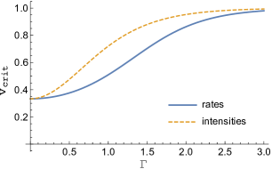
Figure 2: Comparison of critical visibilities to detect entanglement via the Cauchy-like condition, for four-mode squeezed vacuum $\ket{\Psi^{-}}$ mixed with “white” noise in (56). The upper curve is for standard Stokes parameters, and the lower for normalized ones. The latter one turns out to lead to a higher noise resistance. Note that the Cauchy-like condition is equivalent in the case of $\ket{\Psi^{-}}$, and the mixture of $\ket{\Psi^{-}}$ with the model noise, with the necessary and sufficient conditions to detect entanglement via measurement of Stokes parameters. Therefore, this graph shows the critical visibilities also for this case. One cannot do better. Obviously the graphs for $\ket{\Psi^{+}}$, $\ket{\Phi^{+}}$ and $\ket{\Phi^{-}}$ are identical. The asymptotic limit $v_{crit}=1/3$, for $\Gamma\rightarrow 0$, is concurrent with the white noise threshold for a two-qubit singlet.

IV.2 Unitary observables for $d$-mode

Multimode bright squeezed vacuum.—The bright squeezed vacuum is a state of light of undefined photon number which has, due to entanglement, perfect EPR correlations of numbers of photons between specific modes reaching $A$ and $B$. Such an entanglement can be observed in multimode parametric down-conversion emission. The interaction Hamiltonian of the process, for a classical pump, is essentially $\hat{H}=i\gamma\sum_{j=0}^{d-1}\hat{a}_{j}^{\dagger}\hat{b}_{j}^{\dagger}+h.c.$ where $\gamma$ is the coupling constant proportional to a pump power. Thus, $d\times d$ mode (bright) squeezed vacuum state is given by

$$\ket{\Psi_{BSV}^{d}}=\frac{1}{\cosh^{d}\Gamma}\sum_{n=0}^{\infty}\sqrt{\frac{(n+d-1)!}{n!(d-1)!}}\tanh^{n}\Gamma\ket{\psi^{n}_{d}},$$ (70)

where $\Gamma=\gamma t$ and $t$ is the interaction time, and

$$\ket{\psi^{n}_{d}}=\sqrt{\frac{n!(d-1)!}{(n+d-1)!}}\frac{1}{n!}\left(\sum_{j=0}^{d-1}\hat{a}_{j}^{\dagger}\hat{b}_{j}^{\dagger}\right)^{n}\ket{\Omega}.$$ (71)

Noise model.— If we consider the unitary observables, our noise model can look as follows: we build our noise model in following similar steps as for the $d=2$ case. Let us now index $k$ stand for local modes $k=0,1,...,d-1$ and we shall the modulo $d$ algebra for it. Then one can write down the following

$$\ket{\Xi^{d}(m,l)}=\frac{1}{\cosh^{d}\Gamma}\sum_{n=0}^{\infty}\frac{\tanh^{n}{\Gamma}}{n!}\left(\sum_{k}\omega^{km}a^{\dagger}_{k}b^{\dagger}_{k+l}\right)^{n}|\Omega\rangle$$ (72)

with $m$ and $l$ taking values $0,1,...,d-1$. Note that these squeezed $d$-mode vacua are analogs of the following Bell basis for a pair of qudits: $\frac{1}{\sqrt{d}}\sum_{k}\omega^{km}|k\rangle\otimes|k+l\rangle$. Our noise model is defined as

$$\varrho^{noise}=\frac{1}{d^{2}}\sum_{m,l}\outerproduct{\Xi^{d}(m,l)}{\Xi^{d}(m,l)}.$$ (73)

The following properties of the noise are essential for us. For each $i$ and $j$

$$\Tr\hat{Q}_{i}^{A}(m)\hat{Q}_{j}^{B\dagger}(m^{\prime})\varrho^{noise}=0,$$ (74)

and the second property is

$$\Tr(\hat{\Pi}^{A}\hat{\Pi}^{B}\varrho^{noise})=\expectationvalue{\hat{\Pi}^{A}\hat{\Pi}^{B}}{\Psi^{d}_{BSV}}.$$ (75)

We have the same relation for observables based on intensities.

Noise resistance.—Applying this model we get that entanglement detection is possible with the Cauchy-like condition for observables based on rates, in the case of $\ket{\Psi^{d}_{BSV}}$ mixed with the noise, if the threshold visibility $v_{crit}$ fulfills

$$v_{crit}=\frac{\expectationvalue{\hat{\Pi}^{A}}{\Psi^{d}_{BSV}}}{\expectationvalue{\hat{\Pi}^{A}+\hat{\Pi}^{A}\frac{d}{\hat{N}^{A}}\hat{\Pi}^{A}}{\Psi^{d}_{BSV}}}.$$ (76)

In case of observables based on intensities, we get

$$v_{crit}^{old}=\frac{\expectationvalue{(\hat{N}^{A})^{2}}{\Psi^{d}_{BSV}}}{\expectationvalue{\hat{N}^{A}(\hat{N}^{A}+d)}{\Psi^{d}_{BSV}}}.$$ (77)

IV.2.1 $3\times 3$ mode bright squeezed vacuum

In case of observables based on rates, the respective terms in (76) are as follows:

$$\expectationvalue{\hat{\Pi}^{A}\frac{3}{\hat{N}^{A}}\hat{\Pi}^{A}}{\Psi^{3}_{BSV}}$$

$$=\frac{1}{\cosh^{6}\Gamma}9\tanh^{2}\Gamma_{3}F_{2}(1,1,4;2,2;\tanh^{2}\Gamma)$$ (78)

and

$$\expectationvalue{\hat{\Pi}^{A}}{\Psi^{3}_{BSV}}=1-\sech^{6}\Gamma.$$ (79)

For observables based on intensities in (77) we have

$$\expectationvalue{\hat{N}^{A}}{\Psi^{3}_{BSV}}=3\sinh^{2}\Gamma$$ (80)

and

$$\expectationvalue{(\hat{N}^{A})^{2}}{\Psi^{3}_{BSV}} = \frac{1}{\cosh^{6}\Gamma}\frac{3\tanh^{2}\Gamma(3\tanh^{2}\Gamma+1)}{(1-\tanh^{2}\Gamma)^{5}}$$ (81)

$$= 3\sinh^{2}\Gamma+12\sinh^{4}\Gamma$$

The first equality of (81) can be obtained as (here, $x=\tanh^{2}\Gamma$ and $c=\cosh^{6}\Gamma$):

$$\langle(\hat{N}^{A})^{2}\rangle = \frac{1}{c}\sum_{n=0}^{\infty}\frac{(n+1)(n+2)}{2}n^{2}x^{n}$$ (82)

$$= \frac{x}{2c}\frac{d^{2}}{dx^{2}}\bigg{(}\sum_{n=0}^{\infty}n(n+2)x^{n+1}\bigg{)}$$

$$= \frac{x}{2c}\frac{d^{2}}{dx^{2}}\bigg{(}\frac{d}{dx}\bigg{(}\sum_{n=0}^{\infty}nx^{n+2}\bigg{)}\bigg{)}$$

$$= \frac{x}{2c}\frac{d^{3}}{dx^{3}}\bigg{(}x^{3}\frac{d}{dx}\sum_{n=0}^{\infty}x^{n}\bigg{)}$$

$$= \frac{x}{2c}\frac{d^{3}}{dx^{3}}\bigg{(}x^{3}\frac{d}{dx}\bigg{(}\frac{1}{1-x}\bigg{)}\bigg{)}$$

$$= \frac{1}{c}\frac{3x(3x+1)}{(1-x)^{5}}.$$

The threshold visibility in function of the amplification gain, $v_{crit}(\Gamma)$, for the macroscopic singlet $\ket{\Psi^{3}_{BSV}}$ is presented in Fig. 3.

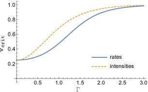
Figure 3: Noise resistance for $\ket{\Psi^{3}_{BSV}}$. Note that for a very weak pumping the visibility approaches $1/4$.

V Derivation of some formulas used in Sec. IV, and to obtain the general Cauchy-like separability condition

V.1 Formula 1

We shall show the following:

$$\sum_{m=0}^{d}\sum_{k=1}^{d-1}|\hat{Q}_{k}(m)|^{2}=(d-1)\left(\hat{\Pi}+\hat{\Pi}\frac{d}{\hat{N}}\hat{\Pi}\right).$$ (83)

Note that this is a generalization of the identity $\sum_{i=1}^{3}\hat{S}_{i}^{2}=\hat{\Pi}+\hat{\Pi}\frac{2}{\hat{N}}\hat{\Pi}$.

The field operators involving the unbiased interferometers, within the approach with rates (15) in the main text can be put as

$$\hat{Q}_{k}(m)=\sum_{l,l^{\prime}=1}^{d}\left(\sum_{j=1}^{d}\omega^{jk}U_{jl^{\prime}}(m)U^{*}_{jl}(m)\right)\hat{\Pi}\frac{a^{\dagger}_{l^{\prime}}a_{l}}{\hat{N}}\hat{\Pi},$$

and the formula for $\hat{Q}_{k}^{\dagger}$ is the Hermitian conjugate of the above. The following relations

$$\sum_{j=1}^{d}{U}_{jl^{\prime}}(m)U^{*}_{jl}(m)\omega^{jk}=[\hat{q}_{k}(m)]_{ll^{\prime}}$$ (84)

and

$$\sum_{j=1}^{d}U^{*}_{jl^{\prime}}(m){U}_{jl}(m)\omega^{-jk}=[{\hat{q}^{\dagger}_{k}(m)}]_{ll^{\prime}}$$ (85)

lead to

$$\hat{Q}_{k}(m)=\sum_{l,l^{\prime}=1}^{d}[\hat{q}_{k}(m)]_{ll^{\prime}}\hat{\Pi}\frac{a^{\dagger}_{l^{\prime}}a_{l}}{\hat{N}}\hat{\Pi},$$ (86)

where $\hat{q}_{k}(m)$ are the qudit operators (40). Therefore, we have

$$\sum_{m=0}^{d}\sum_{k=1}^{d-1}|\hat{Q}_{k}(m)|^{2}=\hat{\Pi}\frac{1}{\hat{N}}\sum_{ll^{\prime}nn^{\prime}=1}^{d}\left(\sum_{m=0}^{d}\sum_{k=1}^{d-1}\right.$$

$$\times[\hat{q}_{k}(m)]_{ll^{\prime}}[{\hat{q}^{\dagger}}_{k}(m)]_{nn^{\prime}}\bigg{)}a^{\dagger}_{l^{\prime}}a_{l}a^{\dagger}_{n}a_{n^{\prime}}\frac{1}{\hat{N}}\hat{\Pi}.$$ (87)

As the operators $\frac{1}{\sqrt{d}}\hat{q}_{k}(m)$ and $\hat{q}_{0}(0)=\openone$ form an orthonormal basis in the Hilbert-Schmidt space of $d\times d$ matrix, we have

$$\delta_{ll^{\prime}}\delta_{nn^{\prime}}+\sum_{m=0}^{d}\sum_{k=1}^{d-1}[\hat{q}_{k}(m)]_{ll^{\prime}}[{\hat{q}^{\dagger}}_{k}(m)]_{nn^{\prime}}=d\delta_{ln}\delta_{l^{\prime}n^{\prime}}.$$

All that, and $[a_{i},a_{j}^{\dagger}]=\delta_{ij}$, allow one to perform the following calculation:

$$\sum_{m=0}^{d}\sum_{k=1}^{d-1}|\hat{Q}_{k}(m)|^{2}$$ (88)

$$= \hat{\Pi}\frac{1}{\hat{N}}\sum_{ll^{\prime}nn^{\prime}=1}^{d}[d\delta_{ln}\delta_{l^{\prime}n^{\prime}}-\delta_{ll^{\prime}}\delta_{nn^{\prime}}]a^{\dagger}_{l^{\prime}}a_{l}a^{\dagger}_{n}a_{n^{\prime}}\frac{1}{\hat{N}}\hat{\Pi}$$

$$= \hat{\Pi}\frac{1}{\hat{N}}\left[-\sum_{ln}a^{\dagger}_{l}a_{l}a^{\dagger}_{n}a_{n}+d\sum_{ll^{\prime}}a^{\dagger}_{l^{\prime}}a_{l}a^{\dagger}_{l}a_{l^{\prime}}\right]\frac{1}{\hat{N}}\hat{\Pi}$$

$$= \hat{\Pi}\frac{1}{\hat{N}}\left[-\hat{N}^{2}+d\sum_{ll^{\prime}}a^{\dagger}_{l^{\prime}}a_{l^{\prime}}(a^{\dagger}_{l}a_{l}+1)-d\sum_{l}a^{\dagger}_{l}a_{l}\right]\frac{1}{\hat{N}}\hat{\Pi}$$

$$= \Pi\frac{1}{\hat{N}}\left[-\hat{N}^{2}+d\hat{N}^{2}+d^{2}\hat{N}-d\hat{N}\right]\frac{1}{\hat{N}}\hat{\Pi}$$

$$= \hat{\Pi}\left[(d-1)+\frac{d(d-1)}{\hat{N}}\right]\hat{\Pi}.$$

Thus, (83) holds.

An analogue relation for the observables involving intensities, which reads

$$\sum_{m=0}^{d}\sum_{k=1}^{d-1}|\hat{\chi}_{k}(m)|^{2}=(d-1)\hat{N}(\hat{N}+d),$$ (89)

can be obtained by similar steps. It is a generalization of (28).

V.2 Formula 2

We here calculate the expressions which enter of Cauchy-Schwartz-like separability conditions based on rates (14) and intensities (16) in the main text for a $d\times d$ mode bright squeezed vacuum. Some of the formulas are also used in the discussion of noise resistance.

Let us consider first the condition (16) in the main text: its LHS and RHS read

$$\rm{LHS} = \sum_{m=0}^{d}\sum_{k=1}^{d-1}\left|\expectationvalue{\hat{\chi}_{{k}}^{A}(m)\hat{\chi}_{{k}}^{{B\dagger}}(m)}{\Psi^{d}_{BSV}}\right|,$$

$$\rm{RHS} = (d-1)\expectationvalue{(\hat{N}^{A})^{2}}{\Psi^{d}_{BSV}}.$$ (90)

To get the formula for RHS we used

$$\expectationvalue{\hat{N}^{A}\hat{N}^{B}}{\Psi^{d}_{BSV}}=\expectationvalue{(\hat{N}^{A})^{2}}{\Psi^{d}_{BSV}}.$$ (91)

The action of $\hat{\chi}_{k}^{B}(m=0)$ on an unnormalized $\ket{\psi^{n}_{d}}$ of (71), which we put as $\ket{\phi^{n}}=\left(\sum_{j=1}^{d}\hat{a}_{j}^{\dagger}\hat{b}_{j}^{\dagger}\right)^{n}\ket{\Omega}$, is as follows

$$\hat{\chi}_{k}^{B}\left(\sum_{j=1}^{d}\hat{a}_{j}^{\dagger}\hat{b}_{j}^{\dagger}\right)^{n}\ket{\Omega}=\left(\sum_{j=1}^{d}\omega^{jk}\hat{b}_{j}^{\dagger}\hat{b}_{j}\right)\left(\sum_{j=1}^{d}\hat{a}_{j}^{\dagger}\hat{b}_{j}^{\dagger}\right)^{n}\ket{\Omega}.$$ (92)

Let us denote as $\hat{X}\equiv\hat{\chi}_{k}^{B}=\sum_{j=1}^{d}\omega^{jk}\hat{b}_{j}^{\dagger}\hat{b}_{j}$ and $\hat{Y}\equiv\sum_{j=1}^{d}\hat{a}_{j}^{\dagger}\hat{b}_{j}^{\dagger}$. Then, we have

$$[\hat{X},\hat{Y}]=\left[\sum_{j=1}^{d}\omega^{jk}\hat{b}_{j}^{\dagger}\hat{b}_{j},\sum_{j=1}^{d}\hat{a}_{j}^{\dagger}\hat{b}_{j}^{\dagger}\right]=\sum_{j=1}^{d}\omega^{jk}\hat{a}_{j}^{\dagger}\hat{b}_{j}^{\dagger}.$$ (93)

Next, we use the algebraic fact that if $[[\hat{X},\hat{Y}],\hat{Y}]=0$, then the following holds $[\hat{X},\hat{Y}^{n}]=n[\hat{X},\hat{Y}]\hat{Y}^{n-1}$ and $\hat{X}\hat{Y}^{n}=\hat{Y}^{n}\hat{X}+n[\hat{X},\hat{Y}]\hat{Y}^{n-1}$. Applying this relation to (92) we get

$${\hat{\chi}}_{k}^{B}\left(\sum_{j=1}^{d}\hat{a}_{j}^{\dagger}\hat{b}_{j}^{\dagger}\right)^{n}\ket{\Omega}=$$

$$n\left(\sum_{j=1}^{d}\omega^{jk}\hat{a}_{j}^{\dagger}\hat{b}_{j}^{\dagger}\right)\left(\sum_{j=1}^{d}\hat{a}_{j}^{\dagger}\hat{b}_{j}^{\dagger}\right)^{n-1}\ket{\Omega},$$ (94)

where we use $\sum_{j=1}^{d}\omega^{jk}\hat{b}_{j}^{\dagger}\hat{b}_{j}\ket{\Omega}=0$. We have the same relation if we replace $\hat{\chi}_{k}^{B}$ by $\hat{\chi}_{k}^{A}$ in (94), i.e.,

$${\hat{\chi}}_{k}^{A}\left(\sum_{j=1}^{d}\hat{a}_{j}^{\dagger}\hat{b}_{j}^{\dagger}\right)^{n}\ket{\Omega}={\hat{\chi}}_{k}^{B}\left(\sum_{j=1}^{d}\hat{a}_{j}^{\dagger}\hat{b}_{j}^{\dagger}\right)^{n}\ket{\Omega}.$$ (95)

The identity (95) holds for all $m=0,1,\dots,d$. In the case of $m\neq 0$ the formulas look the same if one employs creation and annihilation operators related with the interferometers $U(m)$ for $A$ and ${U}^{\dagger}(m)$ for $B$, and the fact that $\sum_{j=1}^{d}\hat{a}_{j}^{\dagger}\hat{b}_{j}^{\dagger}=\sum_{j=1}^{d}\hat{a}_{j}^{\dagger}(m)\hat{b}_{j}^{\dagger}(m)$, which is at the root of EPR correlations of the state. All that, and the identity (89), lead to

LHS $$= \sum_{m=0}^{d}\sum_{k=1}^{d-1}\expectationvalue{|{\hat{\chi}}_{{k}}^{A}(m)|^{2}}{\Psi^{d}_{BSV}}$$ (96)

$$= (d-1)\expectationvalue{\hat{N}^{A}(\hat{N}^{A}+d)}{\Psi^{d}_{BSV}}.$$

Thus, we get

$$\expectationvalue{\hat{N}^{A}(\hat{N}^{A}+d)}{\Psi^{d}_{BSV}}>\expectationvalue{({\hat{N}^{{A}}})^{2}}{\Psi^{d}_{BSV}},$$

for every $\Gamma$.

A reasoning following similar steps leads to a violation of the Cauchy-Schwartz-like separability condition (14) in the main text for observables involving rates, as for the bright squeezed vacuum we have in this case:

$$\expectationvalue{(\hat{\Pi}^{A}+\hat{\Pi}^{A}\frac{d}{\hat{N}^{A}}\hat{\Pi}^{A})}{\Psi^{d}_{BSV}}>\expectationvalue{\hat{\Pi}^{A}}{\Psi^{d}_{BSV}},$$

where $\hat{\Pi}^{A}=(\hat{\Pi}^{A})^{2}$ was used.

V.3 Property (74) of the noise model

The essential property of our noise is that for each $i$ and $j$ we get

$$\Tr\hat{\chi}_{i}^{A}(m)\hat{\chi_{j}}^{B\dagger}(m^{\prime})\varrho^{noise}=0,$$ (99)

and we have the same relation for observables based on rates. We shall prove (99) for $d>2$. For simplicity we will use the intensity approach. The proof for the rate observables is similar.

For an arbitrary $d$ all Bell-like maximally entangled states $\ket{\Xi^{d}(k,l)}$ are linked by a unitary transformation that acts on one subsystem. The transformation is as follows:

$$\hat{\mathcal{U}}^{\dagger}(k,l)\hat{b}^{\dagger}_{n}\hat{\mathcal{U}}(k,l)=\sum_{i=0}^{d-1}U(k,l)_{ni}\hat{b}^{\dagger}_{i}=\omega^{nk}\hat{b}^{\dagger}_{n+l},$$ (100)

where $\hat{b}^{\dagger}_{n}$ stands for $k=0$ and $l=0$. Respectively, for annihilation operators we have: $\hat{\mathcal{U}}^{\dagger}(k,l)\hat{b}_{n}\hat{\mathcal{U}}(k,l)=\sum_{i=0}^{d-1}\bar{U}(k,l)_{ni}\hat{b}_{i}=\omega^{-nk}\hat{b}_{n+l}.$ Using transformation (100) we can present any $\ket{\Xi^{d}(k,l)}$ as follows:

$$\ket{\Xi^{d}(k,l)}$$ (101)

$$= \frac{1}{\cosh^{d}\Gamma}\sum_{n=0}^{\infty}\frac{\tanh^{n}{\Gamma}}{n!}\left(\sum_{m}a^{\dagger}_{m}\hat{\mathcal{U}^{\dagger}}(k,l)b^{\dagger}_{m}\hat{\mathcal{U}}(k,l)\right)^{n}|\Omega\rangle$$

$$= \hat{\mathcal{U}^{\dagger}}(k,l)|\Psi^{d}_{BSV}\rangle.$$

Because this transformation is unitary we can replace the action of (100) on the state by its action on the observables. Thus, in order to prove (99) we shall show that for any $i,j\neq 0$

$$\langle{\Psi_{BSV}^{d}}|\sum_{k,l=0}^{d-1}\hat{\chi}_{i}^{A{}}(m)\hat{\mathcal{U}}(k,l)\hat{\chi}_{j}^{B\dagger}(m^{\prime})\hat{\mathcal{U}}^{\dagger}(k,l)|{\Psi_{BSV}^{d}}\rangle=0.$$ (102)

It turns out that the above holds because of the following operator identity

$$\sum_{k,l=0}^{d-1}\hat{\mathcal{U}}(k,l)\hat{\chi}_{j}^{B\dagger}(m^{\prime})\hat{\mathcal{U}}^{\dagger}(k,l)=0.$$ (103)

The reverse of transformation (100) can be expressed in the following way:

$$\hat{\mathcal{U}}(k,l)\hat{b}^{\dagger}_{n}\hat{\mathcal{U}}^{\dagger}(k,l)=\sum_{i=0}^{d-1}U^{-1}(k,l)_{ni}\hat{b}^{\dagger}_{i}=\omega^{-nk}\hat{b}^{\dagger}_{n-l}.$$ (104)

Note that $U^{-1}$ can be decomposed as follows $U^{-1}=Z^{k}X^{l}$, where $(Z^{k})_{rn}=\delta_{rn}\omega^{-nk}$, $(X^{l})_{ni}=\delta_{(n-l)i}$. Using the notation introduced above we get

$$\hat{\mathcal{U}}(k,l)\hat{\chi}^{B\dagger}_{j}\hat{\mathcal{U}^{\dagger}}(k,l)$$ (105)

$$= \hat{\mathcal{U}}(k,l)\sum_{r=0}^{d-1}\omega^{-rj}\hat{b}^{\dagger}_{r}(m^{\prime})\hat{b}_{r}(m^{\prime})\hat{\mathcal{U}}^{\dagger}(k,l)$$

$$= \sum_{r=0}^{d-1}\omega^{rj}\sum_{s=0}^{d-1}U_{rs}(m^{\prime})\sum_{t=0}^{d-1}(Z^{k}X^{l})_{st}\hat{b}^{\dagger}_{t}$$

$$\times \sum_{s^{\prime}=0}^{d-1}U^{*}_{rs^{\prime}}(m^{\prime})\sum_{t^{\prime}=0}^{d-1}(Z^{k}X^{l})^{*}_{s^{\prime}t^{\prime}}\hat{b}_{t^{\prime}}.$$

We have

$$\sum_{k,l=0}^{d-1}(Z^{k}X^{l})_{st}(\bar{Z}^{k}X^{l})_{s^{\prime}t^{\prime}}$$ (106)

$$= \sum_{k,l=0}^{d-1}\omega^{-sk}\delta_{(s-l)t}\omega^{s^{\prime}k}\delta_{(s^{\prime}-l)t^{\prime}}$$

$$= \sum_{l=0}^{d-1}\delta_{(s-l)t}\delta_{(s^{\prime}-l)t^{\prime}}\sum_{k=0}^{d-1}\omega^{-k(s-s^{\prime})}$$

$$= \delta_{s,s^{\prime}}\delta_{t,t^{\prime}}.$$

Combining (105) and (106) we get

$$\sum_{k,l=0}^{d-1}\hat{\mathcal{U}}(k,l)\hat{\chi}^{B\dagger}_{j}\hat{\mathcal{U}^{\dagger}}(k,l)$$ (107)

$$= \sum_{r=0}^{d-1}\omega^{-rj}\sum_{s,t=0}^{d-1}U_{rs}(m^{\prime})U^{*}_{rs}(m^{\prime})\hat{b}_{t}^{\dagger}\hat{b}_{t}$$

$$= \sum_{r=0}^{d-1}\omega^{-rj}\hat{N}^{B}=0.$$

Thus the identity (103) holds.

References

• (1) J.-W. Pan, Z. B. Chen, C. Y. Lu, H. Weinfurter, A. Zeilinger, and M. Żukowski, Rev. Mod. Phys. 84, 777 (2012).
• (2) A. Aspect, P. Grangier, and G. Roger, Phys. Rev. Lett. 49, 91 (1982).
• (3) D. M. Greenberger, M. A. Horne, and A. Zeilinger, Bell’s Theorem, Quantum Theory, and Conceptions of the Universe, M. Kafatos (Ed.), Kluwer, Dordrecht (1989), 69-72.
• (4) K. Banaszek and K. Wódkiewicz, Phys. Rev. A 58, 4345 (1998); Acta. Phys. Slov. 49, 491-500 (1999).
• (5) C. Simon and D. Bouwmeester, Phys. Rev. Lett. 91, 053601 (2003).
• (6) M. V. Chekhova, G. Leuchs, and M. Żukowski, Opt. Commun. 337, 27 (2015).
• (7) A. Einstein, B. Podolsky, and N. Rosen, Phys. Rev. 47, 777 (1935).
• (8) K. Rosołek, K. Kostrzewa, A. Dutta, W. Laskowski, M. Wieśniak, and M. Żukowski, Phys. Rev. A 95, 042119 (2017).
• (9) G. A. Durkin, C. Simon, and D, Bouwmeester, Phys. Rev. Lett. 88, 187902 (2002).
• (10) R. Horodecki, P. Horodecki, M. Horodecki, and K. Horodecki, Rev. Mod. Phys. 81, 865 (2009).
• (11) R. Simon, Phys. Rev. Lett. 84, 2726 (2000).
• (12) L. -M Duan, et al., Phys. Rev. Lett. 84, 2722 (2000).
• (13) M. Hillery and M. S. Zubairy, Phys. Rev. Lett. 96, 050503 (2006).
• (14) See Supplemental Material at [URL] for more details.
• (15) T. Sh. Iskhakov, I. N. Agafonov, M. V. Chekhova and G. Leuchs, Phys. Rev. Lett. 109, 150502 (2012).
• (16) B. Kanseri, T. Iskhakov, G. Rytikov, M. Chekhova and G. Leuchs, Phys. Rev. A 87, 032110 (2013).
• (17) H. S. Eisenberg, G. Khoury, G. A. Durkin, C. Simon, D. Bouwmeester, Phys. Rev. Lett. 93, 193901 (2004).
• (18) T. Sh. Iskhakov, K. Y. Spasibko, M. V. Chekhova and G. Leuchs, New Journal of Physics 15, 093036 (2013).
• (19) A. Lamas-Linares, J. C. Howell, D. Bouwmeester, Nature 412, 887–890 (2001).
• (20) A. Eckstein, A. Christ, P. J. Mosley and C. Silberhorn, Phys. Rev. Lett. 106, 013603 (2011).
• (21) K. Yu. Spasibko, D. A. Kopylov, V. L. Krutyanskiy, T. V. Murzina, G. Leuchs and M. V. Chekhova, Phys. Rev. Lett. 119, 223603 (2017).
• (22) K. Mattle, M. Michler, H. Weinfurter, A. Zeilinger and M. Żukowski, Appl. Phys. B 60, S111–7 (1995).
• (23) G. Weihs, M. Reck, H. Weinfurter and A. Zeilinger, Phys. Rev. A 54, 893 (1996).
• (24) A. Peruzzo, A. Laing, A. Politi, T. Rudolph and J. L. O’Brien, Nat. Commun. 2, 224 (2011).
• (25) T. Meany, M. Delanty, S. Gross, G. D. Marshall, M. J. Steel and M. J. Withford, Opt. Express 20, 26895 (2012).
• (26) B. J. Metcalf et al. Nat. Commun. 4, 1356 (2013).
• (27) N. Spagnolo, C. Vitelli, L. Aparo, P. Mataloni, F. Sciarrino, A. Crespi, R. Ramponi and R. Osellame, Nat. Commun. 4, 1606 (2013).
• (28) J. Carolan et al., Science 14, 711 (2015).
• (29) C. Schaeff, R. Polster, M. Huber, S. Ramelow and A. Zeilinger, Optica 2, 523 (2015).
• (30) A. Sørensen, L.-M. Duan, J. I. Cirac and P. Zoller, Nature 409, 63 (2001).
• (31) J. Hald, J. L. Sørensen, C. Schori, and E. S. Polzik, Phys. Rev. Lett. 83, 1319 (1999).
• (32) A. S. Sørensen and K. Mølmer, Phys. Rev. Lett. 86, 4431 (2001).
• (33) M. Żukowski, A. Zeilinger and H. Weinfurter, Ann. NY Acad. Sci. 755, 91 (1995).
• (34) R. Kaltenbaek, B. Blauensteiner, M. Żukowski, M. Aspelmeyer, and A. Zeilinger, Phys. Rev. Lett. 96, 240502 (2006).
• (35) M. Żukowski, W. Laskowski, and M. Wieśniak, Phys. Rev. A 95, 042113 (2017).
• (36) M. Żukowski, W. Laskowski, and M. Wieśniak, Phys. Scr. 91, 084001 (2016).
• (37) M. Żukowski, M. Wieśniak, and W. Laskowski, Phys. Rev. A 94, 020102(R) (2016).
• (38) Q. Y. He, M. D. Reid, T. G. Vaughan, C. Gross, M. Oberthaler, and P. D. Drummond, Phys. Rev. Lett. 106, 120405 (2011); Q. Y. He, T. G. Vaughan, P. D. Drummond, and M. D. Reid, New Journal of Physics 14, 093012 (2012).
• (39) M. Reck, A. Zeilinger, H. J. Bernstein, and P. Bertani, Phys. Rev. Lett. 73, 58 (1994).
• (40) W. K. Wootters and B. D. Fields, Ann. Phys. 191, 363 (1989).
• (41) I. D. Ivanovic, J. Phys. A: Math. Theor. 14, 3241 (1981).
• (42) N. Brunner, D. Cavalcanti, S. Pironio, V. Scarani, and S. Wehner, Rev. Mod. Phys. 86, 419 (2014).
• (43) R. Schmied, J.-D. Bancal, B. Allard, M. Fadel, V. Scarani, P. Treutlein, and N. Sangouard, Science 352, 441 (2016).
• (44) J. Ryu, M. Marciniak, M. Wieśniak, and M. Żukowski, J. Opt. 20, 044002 (2018).
• (45) J. Ryu, M. Marciniak, M. Wieśniak, D. Kaszlikowski, and M. Żukowski, Acta Phys. Pol. A 132, 1713 (2017).
• (46) S. Yu, J.-W. Pan, Z.-B. Chen, and Y.-D. Zhang, Phys. Rev. Lett. 91, 217903 (2003).
• (47) J.  M. Jauch and F. Rohrlich, The Theory of Photons and Electrons (Addison-Wesley, Reading, MA, 1955).