Optimization methods for MR image reconstruction
(Long version)

Abstract

The development of compressed sensing methods[1] for magnetic resonance (MR) image reconstruction[2] led to an explosion of research on models and optimization algorithms for MR imaging (MRI). Roughly 10 years after such methods first appeared in the MRI literature[3], the U.S. Food and Drug Administration (FDA) approved certain compressed sensing methods for commercial use[4, 5, 6], making compressed sensing a clinical success story for MRI. This review paper summarizes several key models and optimization algorithms for MR image reconstruction, including both the type of methods that have FDA approval for clinical use, as well as more recent methods being considered in the research community that use data-adaptive regularizers. Many algorithms have been devised that exploit the structure of the system model and regularizers used in MRI; this paper strives to collect such algorithms in a single survey. Many of the ideas used in optimization methods for MRI are also useful for solving other inverse problems.

I Introduction

I-A Scope

Although the paper title begins with “optimization methods,” in practice one first defines a model and cost function, and then applies an optimization algorithm. There are several ways to partition the space of models, cost functions and optimization methods for MRI reconstruction, such as: smooth vs non-smooth cost functions, static vs dynamic problems, single-coil vs multiple-coil data. This paper focuses on the static reconstruction problem because the dynamic case is rich enough to merit its own survey paper[7]. This paper emphasizes algorithms for multiple-coil data (parallel MRI[8, 9]) because modern systems all have multiple channels and advanced reconstruction methods with under-sampling are most likely to be used for parallel MRI scans. Main families of parallel MRI methods include “SENSE” methods that model the coil sensitivities in the image domain [10, 11], “GRAPPA” methods that model the effect of coil sensitivity in k-space [12], and “calibrationless” methods that use low-rank or joint sparsity properties [13, 14, 15, 16]. This paper considers all three approaches, emphasizing SENSE methods for simplicity.

I-B Measurement model

The signals recorded by the sensors (receive coils) in MR scanners are linear functions of the object’s transverse magnetization. That magnetization is a complicated and highly nonlinear function of the RF pulses, gradient waveforms, and tissue properties, governed by the physics of the Bloch equation [18, 19, 20]. Quantifying tissue properties using nonlinear models is a rich topic of its own[21][22, 23, 24, 25], but we focus here on the problem of reconstructing images of the transverse magnetization from MR measurements.

Ignoring noise, a vector $\mathop{{}\bm{s}}\nolimits\in\mathbb{C}^{M}$ of signal samples recorded by a MR receive coil is related (typically) to a discretized version $\bm{x}\in\mathbb{C}^{N}$ of the transverse magnetization via a linear Fourier relationship:

$$\mathop{{}\bm{s}}\nolimits=\bm{F}\bm{x},\quad F_{ij}=\mathop{{}{\operator@font exp}}\nolimits\left(-\imath 2\pi\vec{\nu}_{i}\cdot\vec{\mathrm{x}}_{j}\right),\ \begin{array}[]{c}i=1,\ldots,M\\ j=1,\ldots,N,\end{array}$$ (1)

where $\vec{\nu}_{i}$ denotes the k-space sample location of the $i$th sample (units cycles/cm) and $\vec{\mathrm{x}}_{j}$ denotes the spatial coordinates of the center of the $j$th pixel (units cm). In the usual case where the pixel coordinates $\left\{\vec{\mathrm{x}}_{j}\right\}$ and k-space sample locations $\left\{\vec{\nu}_{i}\right\}$ are both on appropriate Cartesian grids, matrix $\bm{F}$ is square corresponds to the (2D or 3D) discrete Fourier transform (DFT). In this case $\bm{F}^{-\!1}=\frac{1}{N}\bm{F}^{\prime}$ so reconstructing $\bm{x}$ from $\mathop{{}\bm{s}}\nolimits$ is simply an inverse fast Fourier transform (FFT), and that approach is used in many clinical MR scans.

The reconstruction problem becomes more interesting when the k-space sample locations are on a non-Cartesian grid[11, 26], when the scan is “accelerated” by recording $M<N$ samples, when non-Fourier effects like magnetic field inhomogeneity are considered [27] and/or when there are multiple receive coils. In parallel MRI, let $\mathop{{}\bm{s}_{l}}\nolimits$ denote the samples recorded by the $l$th of of $L$ receive coils. Then one replaces the model (1) with

$$\mathop{{}\bm{s}_{l}}\nolimits=\bm{F}\bm{C}_{l}\bm{x},$$ (2)

where $\bm{C}_{l}$ is a $N\times N$ diagonal matrix containing the coil sensitivity pattern of the $l$ coil on its diagonal. Note that $\bm{F}$ does not depend on $l$; all coils see the same k-space sampling pattern. Stacking up the measurements from all coils and accounting for noise yields the following basic forward model in MRI:

$$\begin{bmatrix}\bm{y}_{1}\\ \vdots\\ \bm{y}_{L}\end{bmatrix}=\bm{y}=\underbrace{(\bm{I}_{L}\otimes\bm{F})\bm{C}}_{\mbox{$\bm{A}$}}\bm{x}+\bm{\varepsilon},\ \bm{C}=\begin{bmatrix}\bm{C}_{1}\\ \vdots\\ \bm{C}_{L}\end{bmatrix},$$ (3)

where $\bm{A}\in\mathbb{C}^{ML\times N}$ denotes the system matrix, $\bm{y}\in\mathbb{C}^{ML}$ denotes the measured k-space data, and $\bm{x}\in\mathbb{C}^{N}$ denotes the latent image. The noise in k-space is well modeled as complex white Gaussian noise[28]. For extensions that consider other physics effects like relaxation and field inhomogeneity, see [19].

The goal in MR image reconstruction is to recover $\bm{x}$ from $\bm{y}$ using the model (3). All MR image reconstruction problems are under-determined because the magnetization of the underlying object being scanned is a space-limited continuous-space function on $\mathbb{R}^{3}$, yet only a finite number of samples are recorded. Nevertheless, the convention in MRI is to treat the object as a finite-dimensional vector $\bm{x}\in\mathbb{C}^{N}$ for which $M\geq N$ appropriate Cartesian k-space samples is considered “fully sampled” and any $M<N$ is considered “accelerated.” The term “compressed sensing” [29] in this setting might simply mean that the k-space sampling is $\bm{A}$ is a wide matrix, i.e., $LM<N$, or might imply that the sampling pattern satisfies some sufficient condition for ensuring good recovery of $\bm{x}$ from $\bm{y}$. Sampling pattern design is a topic of ongoing interest [30, 31, 32], with renewed interest in data-driven methods [33, 34, 35]. One MRI vendor uses a spiral phyllotaxis sampling pattern for 3D imaging [36] that emphasizes the center of k-space.

The matrix $\bm{F}$ in (3) is known prior to the scan, because the k-space sample locations $\left\{\vec{\nu}_{i}\right\}$ are controlled by the pulse sequence designer. (Calibration methods are sometimes needed for complicated k-space sampling patterns [37].) In contrast, the coil sensitivity maps $\left\{\bm{C}_{l}\right\}$ depend on the exact configuration of the receive coils for each patient. To use the model (3), one must determine the sensitivity maps from some patient-specific calibration data, e.g., by joint estimation [38, 39, 40, 41, 42], regularization[3][43], or subspace methods [44].

II Cost functions and algorithms

II-A Quadratic problems

When $ML\geq N$, i.e., when the total number of k-space samples acquired across all coils exceeds the number of unknown image pixel values, the linear model (3) is over-determined. If additionally $\bm{A}$ is well conditioned, which depends on the sampling pattern and coil sensitivity maps, then it is reasonable to consider an ordinary least-squares estimator

$$\mathop{{}\hat{\bm{x}}}\nolimits =\operatorname*{arg\,min}_{\bm{x}\in\mathbb{C}^{N}}\frac{1}{2}\left\|\bm{A}\bm{x}-\bm{y}\right\|_{2}^{2}=(\bm{A}^{\prime}\bm{A})^{-\!1}\bm{A}^{\prime}\bm{y}$$

$$=\left(\textstyle\sum_{l=1}^{L}\bm{C}_{l}^{\prime}\bm{F}^{\prime}\bm{F}\bm{C}_{l}\right)^{-\!1}\left(\textstyle\sum_{l=1}^{L}\bm{C}_{l}^{\prime}\bm{F}^{\prime}\bm{y}\right).$$ (4)

In particular, for fully sampled Cartesian k-space data where $\bm{F}^{-\!1}=\frac{1}{N}\bm{F}^{\prime},$ this least-squares solution simplifies to $\mathop{{}\hat{\bm{x}}}\nolimits=\left(\sum_{l=1}^{L}\bm{C}_{l}^{\prime}\bm{C}_{l}\right)^{-\!1}\left(\sum_{l=1}^{L}\bm{C}_{l}^{\prime}\bm{F}^{-\!1}\bm{y}\right),$ which is trivial to implement because each $\bm{C}_{l}$ is diagonal. This is known as the optimal coil combination approach [8]. For regularly under-sampled Cartesian data, where only every $n$th row of k-space is collected, the matrix $\bm{F}^{\prime}\bm{F}$ has a simple block structure with $n\times n$ blocks that facilitates non-iterative block-wise computation known as SENSE reconstruction [10]. This form of least-squares estimation is used widely in clinical MR systems.

II-B Regularized least-squares

For under-sampled problems $(ML<N)$ the LS solution (4) is not unique. Furthermore, even when $ML\geq N$ often $\bm{A}$ is poorly conditioned, particularly for non-Cartesian sampling. Some form of regularization is needed in such cases. Some early MRI reconstruction work used quadratically regularized cost functions leading to optimization problems of the form:

$$\mathop{{}\hat{\bm{x}}}\nolimits=\operatorname*{arg\,min}_{\bm{x}\in\mathbb{C}^{N}}\frac{1}{2}\left\|\bm{A}\bm{x}-\bm{y}\right\|_{2}^{2}+\upbeta\left\|\bm{T}\bm{x}\right\|_{2}^{2},$$ (5)

where $\upbeta>0$ denotes a regularization parameter and $\bm{T}$ denotes a $K\times N$ matrix transform such as finite differences. Some methods based on annihilation filters also have this form [47]. The conjugate gradient (CG) algorithm is well-suited to such quadratic cost functions [11, 27]. The Hessian matrix $\bm{A}^{\prime}\bm{A}+\upbeta\bm{T}^{\prime}\bm{T}$ often is approximately Toeplitz [48, 49], so CG with circulant preconditioning is particularly effective[50]. Although the quadratically regularized least-squares cost function (5) is passé in the compressed sensing era, CG is often an inner step for optimizing more complicated cost functions[51][45].

II-C Edge-preserving regularization

The drawback of the quadratically regularized cost function (5) with $\bm{T}$ as finite differences is that it blurs image edges. To avoid this blur, one can replace the quadratic regularizer $\left\|\bm{T}\bm{x}\right\|_{2}^{2}$ with a nonquadratic function $\mathop{{}\psi\left(\bm{T}\bm{x}\right)}\nolimits$ where typically $\mathop{{}\psi}\nolimits$ is convex and smooth, such as the Huber function[52], a hyperbola[53, 54], or the Fair potential function $\mathop{{}\psi\left(z\right)}\nolimits=\delta^{2}\left(\left|z/\delta\right|-\mathop{{}{\operator@font log}\left(1+\left|z/\delta\right|\right)}\nolimits\right),$ among others [55, Ch. 2] as follows:

$$\mathop{{}\hat{\bm{x}}}\nolimits=\operatorname*{arg\,min}_{\bm{x}\in\mathbb{C}^{N}}\mathop{{}\Psi\left(\bm{x}\right)}\nolimits\triangleq\frac{1}{2}\left\|\bm{A}\bm{x}-\bm{y}\right\|_{2}^{2}+\upbeta\mathop{{}\psi\left(\bm{T}\bm{x}\right)}\nolimits.$$ (6)

Such methods have their roots in Bayesian methods based on Markov random fields[56, 57]. The nonlinear CG algorithm is an effective optimization method for cost functions with such smooth edge-preserving regularizers. An interesting alternative is the complex-valued 3MG (majorize-minimize memory gradient) algorithm [54]. Another appropriate optimization algorithm is the optimized gradient method (OGM)[58], a first-order method having optimal worst-case performance among all first-order algorithms for convex cost functions with Lipschitz continuous gradients[59]. OGM has a convergence rate bound that is twice better than that of Nesterov’s fast gradient method[60]. A recent line-search OGM variant is even more attractive [61].

Fig. 1 compares two of these methods for the case where $\bm{T}$ is finite differences and $\mathop{{}\psi}\nolimits$ is the Fair potential with $\delta=0.1$, which approximates TV fairly closely while being smooth.

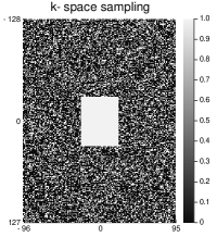
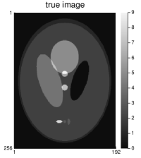
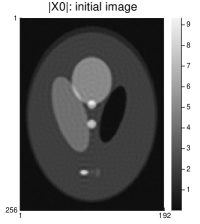
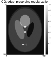
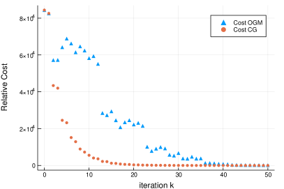
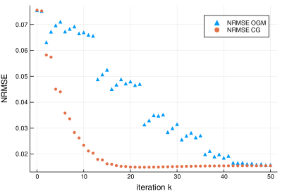
Figure 1: Comparison of CG and OGM convergence for single-coil MRI reconstruction with edge-preserving regularization (akin to anisotropic TV with corner rounding). From left to right: Top row: k-space sampling pattern where only 34% of the phase-encodes are collected, true image, initial image from zero-filled k-space data, minimizer $\mathop{{}\hat{\bm{x}}}\nolimits$ of (6). (Both CG and OGM converge to the same limit $\mathop{{}\hat{\bm{x}}}\nolimits$.) Bottom row: cost function $\mathop{{}\Psi\left(\bm{x}_{k}\right)}\nolimits$ in (6) and normalized root mean squared error (NRMSE) $\left\|\bm{x}_{k}-\bm{x}\right\|_{2}/\left\|\bm{x}\right\|_{2}$ versus iteration $k$.

II-D Sparsity models: synthesis form

Scan time in MRI is proportional to the number of k-space samples recorded. Reducing scan time in MRI can reduce cost, improve patient comfort, and reduce motion artifacts. Reducing the number of k-space samples $ML$ to well below $N$, necessitates stronger modeling assumptions about $\bm{x}$, and sparsity models are prevalent [62] [2]. Two main categories of sparsity models are the synthesis approach and the analysis approach. In a synthesis model, one assumes $\bm{x}=\bm{B}\bm{z}$ for some $N\times K$ matrix $\bm{B}$ where coefficient vector $\bm{z}\in\mathbb{C}^{K}$ should be sparse. In an analysis model, one assumes $\bm{T}\bm{x}$ is sparse, for some $K\times N$ transformation matrix $\bm{T}$.

A typical cost function for a synthesis model is

$$\mathop{{}\hat{\bm{x}}}\nolimits=\bm{B}\hat{\bm{z}},\quad\hat{\bm{z}}=\operatorname*{arg\,min}_{\bm{z}\in\mathbb{C}^{K}}\frac{1}{2}\left\|\bm{A}\bm{B}\bm{z}-\bm{y}\right\|_{2}^{2}+\upbeta\left\|\bm{z}\right\|_{1},$$ (7)

where the 1-norm is a convex relaxation of the $\ell_{0}$ counting measure that encourages $\bm{z}$ to be sparse. Typically $\bm{B}$ is a wide matrix (often called an over-complete dictionary) so that one can represent $\bm{x}$ well using only a fraction of the columns of $\bm{B}$. The optimization formulation (7) is also known as the LASSO problem [63, 64] and there are numerous algorithms for solving it. The classical approach for (7) is the iterative soft thresholding algorithm (ISTA)[65], also known as the proximal gradient method (PGM) [66] and proximal forward-backward splitting[67], having the simple form

$$\bm{z}_{k+1}=\text{soft}\left(\bm{z}_{k}-\bm{D}^{-\!1}\bm{B}^{\prime}\bm{A}^{\prime}(\bm{A}\bm{B}\bm{z}_{k}-\bm{y}),\upbeta/\bm{d}\right),$$ (8)

where the soft thresholding function is defined by $\text{soft}(z,c)=\mathop{{}{\operator@font sign}\left(z\right)}\nolimits\max(\left|z\right|-c,0)$ and $\bm{D}=\mathop{{}\mathsf{diag}\left\{\bm{d}\right\}}\nolimits$ is any positive definite diagonal matrix such that $\bm{D}-\bm{B}^{\prime}\bm{A}^{\prime}\bm{A}\bm{B}$ is positive semidefinite[68].

The ISTA update (8) applies to the 1-norm in (7). If we replace that 1-norm with some other function $\mathop{{}\psi\left(\bm{z}\right)}\nolimits$, then one replaces (8) with the more general PGM update of the form

$$\bm{z}_{k+1}=\text{prox}_{\upbeta\mathop{{}\psi}\nolimits}\left(\bm{z}_{k}-\bm{D}^{-\!1}\bm{B}^{\prime}\bm{A}^{\prime}(\bm{A}\bm{B}\bm{z}_{k}-\bm{y}),\upbeta/\bm{d}\right),$$

where the proximal operator is defined by

$$\mathop{{}{\operator@font prox}_{f}\left(\mathop{{}\bm{v}}\nolimits\right)}\nolimits\triangleq\operatorname*{arg\,min}_{\bm{x}}\frac{1}{2}\left\|\bm{x}-\mathop{{}\bm{v}}\nolimits\right\|_{2}^{2}+f(\bm{x}).$$

Traditionally $\bm{D}=|\!|\!|\bm{B}^{\prime}\bm{A}^{\prime}\bm{A}\bm{B}|\!|\!|_{2}\bm{I},$ but computing that spectral norm (via the power iteration) requires considerable computation for parallel MRI problems in general. However, for Cartesian sampling, $\bm{F}^{\prime}\bm{F}\preceq N\bm{I}$ so it suffices to have $N\bm{B}^{\prime}\bm{C}^{\prime}\bm{C}\bm{B}\preceq\bm{D}.$ Often the sensitivity maps are normalized such that $\bm{C}^{\prime}\bm{C}=\bm{I}$ in which case $N\bm{B}^{\prime}\bm{B}\preceq\bm{D}$ suffices. If in addition $\bm{B}^{\prime}$ is a Parseval tight frame, then $\bm{B}^{\prime}\bm{B}\preceq\bm{I}$ so using $\bm{D}=N\bm{I}$ is appropriate. For non-Cartesian sampling, or non-normalized sensitivity maps, or general choices of $\bm{B}$, finding $\bm{D}$ is more complicated[68].

Although ISTA is simple, it has an undesirably slow $O(1/k)$ convergence bound, where $k$ denotes the number of iterations. This limitation was first overcome by the fast iterative soft thresholding algorithm (FISTA) [69, 70], also known as the fast proximal gradient method (FPGM) that has an $O(1/k^{2})$ convergence bound. A recent extension of this line of proximal methods is the proximal optimized gradient method (POGM) that has worst-case convergence bound about twice better than that of FISTA/FPGM[71, 72]. Both FISTA and POGM are essentially as simple to implement as (8). Recent MRI studies have shown POGM converging faster than FISTA, as one would expect based on the convergence bounds[73, 74], particularly when combined with adaptive restart [71, 75]. So POGM (with restart) is a recommended method for optimization problems having the form (7). This topic remains an active research area with new variants of FISTA appearing recently [76]. Table 3 provides POGM pseudo-code for solving composite optimization problems like the MRI synthesis reconstruction model (7).

Fig. 2 shows that POGM converges faster than FISTA and ISTA for minimizing (7).

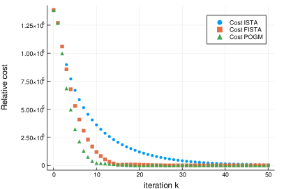
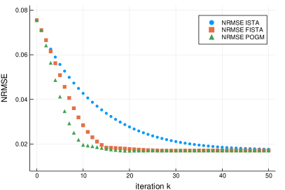
Figure 2: Comparison of ISTA/PGM, FISTA/FPGM and POGM for single-coil MRI reconstruction with orthogonal discrete wavelet transform sparsity regularizer using the 1-norm. Minimizer $\mathop{{}\hat{\bm{x}}}\nolimits$ of (7); cost function for (7); NRMSE versus iteration $k$. FISTA requires about 40% more iterations to converge than POGM, consistent with the $2\times$ better worst-case bound of POGM.

Initialize $\bm{w}_{0}=\bm{x}_{0},$ $\theta_{0}=1.$ Then for $k=1:N$:

$$\theta_{k} =\left\{\begin{array}[]{ll}\frac{1}{2}\left(1+\sqrt{4\theta_{k-1}^{2}+1}\right),&k<N\\ \frac{1}{2}\left(1+\sqrt{8\theta_{k-1}^{2}+1}\right),&k=N\end{array}\right.$$

$$\gamma_{k} =\frac{1}{L}\frac{2\theta_{k-1}+\theta_{k}-1}{\theta_{k}}$$

$$\bm{w}_{k} =\bm{x}_{k-1}-\frac{1}{L}\nabla f(\bm{x}_{k-1})$$

$$\bm{z}_{k} =\bm{w}_{k}+\frac{\theta_{k-1}-1}{\theta_{k}}(\bm{w}_{k}-\bm{w}_{k-1})+\frac{\theta_{k-1}}{\theta_{k}}(\bm{w}_{k}-\bm{x}_{k-1})$$

$$\hskip 20.00003pt+\frac{\theta_{k-1}-1}{L\gamma_{k-1}\theta_{k}}(\bm{z}_{k-1}-\bm{x}_{k-1})$$

$$\bm{x}_{k} =\mathop{{}{\operator@font prox}_{\gamma_{k}g}\left(\bm{z}_{k}\right)}\nolimits=\operatorname*{arg\,min}_{\bm{x}}\frac{1}{2}\left\|\bm{x}-\bm{z}_{k}\right\|_{2}^{2}+\gamma_{k}g(\bm{x})$$

Figure 3: POGM method [72] for minimizing $f(\bm{x})+g(\bm{x})$ where $f$ is convex with $L$-Lipschitz smooth gradient and $g$ is convex. See [71] for adaptive restart version.

II-E Sparsity models: analysis form

A potential drawback of the synthesis formulation (7) is that $\bm{x}\approx\bm{B}\bm{z}$ may be a more realistic assumption than the strict equality $\bm{x}=\bm{B}\bm{z}$ when $\bm{z}$ is sparse. The analysis approach avoids constraining $\mathop{{}\hat{\bm{x}}}\nolimits$ to lie in any such subspace (or union of subspaces when $\bm{B}$ is wide). For an analysis form sparsity model, a typical optimization problem involves a composite cost function consisting of the sum of a smooth term and a non-smooth term:

$$\mathop{{}\hat{\bm{x}}}\nolimits=\operatorname*{arg\,min}_{\bm{x}}\frac{1}{2}\left\|\bm{A}\bm{x}-\bm{y}\right\|_{2}^{2}+\upbeta\left\|\bm{T}\bm{x}\right\|_{1},$$ (9)

where $\bm{T}$ is a sparsifying operator such as a wavelet transform, or finite differences, or both [62]. The expression (9) is general enough to handle combinations of multiple regularizers, such as wavelets and finite differences [2], by stacking the operators in $\bm{T}$ and possibly allowing a weight 1-norm. When $\bm{T}$ is finite differences, the regularizer is called total variation (TV)[3], and combinations of TV and wavelet transforms are useful [2]. Although the details are proprietary, the FDA-approved method for compressed sensing MRI for at least one manufacturer is related to (9)[77] [78].

We write an ordinary 1-norm in (9), but some clinical MRI scanners use a weighted norm that regularizes the high-frequency components more [79].

When $\bm{T}$ is invertible, such as an orthogonal wavelet transform, one rewrites the optimization problem (9) as

$$\mathop{{}\hat{\bm{x}}}\nolimits=\bm{T}^{-\!1}\hat{\bm{z}},\quad\hat{\bm{z}}=\operatorname*{arg\,min}_{\bm{z}}\frac{1}{2}\left\|\bm{A}\bm{T}^{-\!1}\bm{z}-\bm{y}\right\|_{2}^{2}+\upbeta\left\|\bm{z}\right\|_{1},$$

which is simply a special case of (7) with $\bm{B}=\bm{T}^{-\!1}$. Typically $\bm{B}$ is wide and $\bm{T}$ is tall so this simplification is not possible in general.

In the general case (9) where $\bm{T}$ is not invertible, the optimization problem is much harder than (7) due to the non-differentiability of the 1-norm with the matrix $\bm{T}$. The non-invertible case (with redundant Haar wavelets) is used clinically [79, 80][78]. The PGM for (9) is

$$\bm{x}_{k+1}=\operatorname*{arg\,min}_{\bm{x}}\frac{\mathcal{L}}{2}\left\|\bm{x}-\tilde{\bm{x}}_{k}\right\|_{2}^{2}+\upbeta\left\|\bm{T}\bm{x}\right\|_{1},$$ (10)

where $\tilde{\bm{x}}_{k}\triangleq\bm{x}_{k}-\frac{1}{\mathcal{L}}\bm{A}^{\prime}(\bm{A}\bm{x}_{k}-\bm{y})$ denotes the usual gradient update and the Lipschitz constant is $\mathcal{L}=|\!|\!|\bm{A}|\!|\!|_{2}^{2}$. Unfortunately there is no simple solution for computing the proximal operator (defined after (8) above) in (10) in general, so inner iterative methods are required, typically involving dual formulations[81][69]. This challenge makes PGM and FPGM and POGM less attractive for (9) and has led to a vast literature on algorithms for problems like (9), with no consensus on what is best. The difficulty of (10) is the main drawback of analysis regularization, whereas a possible drawback of the synthesis regularization in (7) is that often $K\gg N$ for overcomplete $\bm{B}$.

II-E1 Approximate methods

One popular “work around” option is to “round the corner” of the 1-norm, making smooth approximations like $\left|z\right|\approx\sqrt{\left|z\right|^{2}+\epsilon}.$ This approximation is simply the hyperbola function that has a long history in the edge-preserving regularization literature. All of the gradient-based algorithms mentioned for edge-preserving regularization above are suitable candidates when a smooth function replaces the 1-norm. Smooth functions can shrink values towards zero, but their proximal operators never have a thresholding effect that induces sparsity by setting many values exactly to zero. Whether a thresholding effect is truly essential is an open question.

One way to overcome the challenge of the matrix $\bm{T}$ in the 1-norm in (9) is to replace (9) with the following alternative [82]:

$$\mathop{{}\hat{\bm{x}}}\nolimits =\operatorname*{arg\,min}_{\bm{x}}\frac{1}{2}\left\|\bm{A}\bm{x}-\bm{y}\right\|_{2}^{2}+\upbeta R_{\alpha}(\bm{x})$$

$$R_{\alpha}(\bm{x}) =\min_{\bm{z}}\frac{1}{2}\left\|\bm{T}\bm{x}-\bm{z}\right\|_{2}^{2}+\alpha\left\|\bm{z}\right\|_{1}$$ (11)

where $\alpha>0$. At first glance this formulation appears to enforce sparsity due to the presence of the 1-norm. However, one can solve for $\bm{z}$ and substitute back in to show that $R_{\alpha}(\bm{x})=\mathop{{}\psi\left(\bm{T}\bm{x},\alpha\right)}\nolimits$ where $\mathop{{}\psi}\nolimits$ is the Huber function with parameter $\alpha$, so (11) is simply another example of corner rounding with an approximate 1-norm. One can show $\frac{1}{\alpha}R_{\alpha}(\bm{x})\rightarrow\left\|\bm{T}\bm{x}\right\|_{1}$ as $\alpha\rightarrow 0$. A drawback of (11) is that one must choose the additional regularization parameter $\alpha$ that can affect both the image quality of $\mathop{{}\hat{\bm{x}}}\nolimits$ and the convergence rate of iterative algorithms for (11).

Another option is to use an iterative reweighted least-squares approach like FOCUSS [83] that approaches the 1-norm in the limit as the number of iterations grows, but is effectively equivalent to a corner-rounded 1-norm for any finite number of iterations. Hereafter we focus on methods that tackle the 1-norm directly without any such approximations.

II-E2 Variable splitting methods

Variable splitting methods replace (9) with an exactly equivalent constrained minimization problem involving an auxiliary variable such as $\bm{z}=\bm{T}\bm{x}$, e.g.,

$$\mathop{{}\hat{\bm{x}}}\nolimits=\operatorname*{arg\,min}_{\bm{x}}\min_{\bm{z}\,:\,\bm{z}=\bm{T}\bm{x}}\frac{1}{2}\left\|\bm{A}\bm{x}-\bm{y}\right\|_{2}^{2}+\upbeta\left\|\bm{z}\right\|_{1}.$$ (12)

This approach underlies the split Bregman algorithm[84], various augmented Lagrangian methods [45, 51], and the alternating direction multiplier method (ADMM) [85]. The augmented Lagrangian for (12) is

$$L(\bm{x},\bm{z};\bm{\gamma},\mu) =\frac{1}{2}\left\|\bm{A}\bm{x}-\bm{y}\right\|_{2}^{2}+\upbeta\left\|\bm{z}\right\|_{1}$$

$$+\mathop{{}{\operator@font real}\left\{\mathop{\langle\bm{\gamma},\,\bm{T}\bm{x}-\bm{z}\rangle}\nolimits\right\}}\nolimits+\frac{\mu}{2}\left\|\bm{T}\bm{x}-\bm{z}\right\|_{2}^{2},$$

where $\bm{\gamma}\in\mathbb{C}^{K}$ denotes the vector of Lagrange multipliers  and $\mu>0$ is an AL penalty parameter that affects the convergence rate but not the final image $\mathop{{}\hat{\bm{x}}}\nolimits$. Defining the scaled dual variable $\bm{\eta}\triangleq 1/\mu\bm{\gamma}$ and completing the square leads to the following scaled augmented Lagrangian:

$$L(\bm{x},\bm{z};\bm{\eta},\mu) =\frac{1}{2}\left\|\bm{A}\bm{x}-\bm{y}\right\|_{2}^{2}+\upbeta\left\|\bm{z}\right\|_{1}$$

$$\hskip 20.00003pt+\frac{\mu}{2}\left(\left\|\bm{T}\bm{x}-\bm{z}+\bm{\eta}\right\|_{2}^{2}-\left\|\bm{\eta}\right\|_{2}^{2}\right).$$

An augmented Lagrangian approach alternates between descent updates of the primal variables $\bm{x}$, $\bm{z}$ and an ascent update of the scaled dual variable $\bm{\eta}$. The $\bm{z}$ update is simply soft thresholding:

$$\bm{z}_{k+1}=\text{soft}(\bm{T}\bm{x}_{k}+\bm{\eta}_{k},\upbeta/\mu).$$

The $\bm{x}$ update minimizes a quadratic function:

$$\bm{x}_{k+1}=(\bm{A}^{\prime}\bm{A}+\mu\bm{T}^{\prime}\bm{T})^{-\!1}(\bm{A}^{\prime}\bm{y}+\mu\bm{T}^{\prime}(\bm{z}_{k+1}+\bm{\eta}_{k})).$$

A few CG iterations (with an appropriate preconditioner) is a natural choice for approximating the $\bm{x}$ update. Finally the $\bm{\eta}$ update is

$$\bm{\eta}_{k+1}=\bm{\eta}_{k}+(\bm{T}\bm{x}_{k+1}-\bm{z}_{k+1}).$$

The unit step size here ensures dual feasibility [86]. A drawback of variable splitting methods is the need to select the parameter $\mu$. Adaptive methods have been proposed to help with this tuning[86][87, 88]. The above updates of $\bm{x}$ and $\bm{z}$ are sequential; parallel ADMM updates are also possible [89, 90].

One could apply ADMM to the synthesis regularized problem (7), though again it would require parameter tuning that is unnecessary with POGM.

The conventional variable split in (12) ignores the specific structure of the MRI system matrix $\bm{A}$ in (3). Important properties of $\bm{A}$ include the fact that $\bm{F}^{\prime}\bm{F}$ is circulant (for Cartesian sampling) or Toeplitz (for non-Cartesian sampling) and that each coil sensitivity matrix $\bm{C}_{l}$ is diagonal. In contrast, the Gram matrix $\bm{A}^{\prime}\bm{A}$ for parallel MRI is harder to precondition, though possible[91, 92]. An alternative splitting that simplifies the updates is [45]:

$$\operatorname*{arg\,min}_{\bm{x}\in\mathbb{C}^{N}}\min_{\mathop{{}\bm{u}}\nolimits\in\mathbb{C}^{NL},\,\bm{z}\in\mathbb{C}^{K},\,\mathop{{}\bm{v}}\nolimits\in\mathbb{C}^{N}}\frac{1}{2}\left\|\bm{F}_{L}\mathop{{}\bm{u}}\nolimits-\bm{y}\right\|_{2}^{2}+\upbeta\left\|\bm{z}\right\|_{1}$$

$$\text{ sub. to }\mathop{{}\bm{u}}\nolimits=\bm{C}\bm{x},\ \bm{z}=\bm{T}\mathop{{}\bm{v}}\nolimits,\ \mathop{{}\bm{v}}\nolimits=\bm{x},$$ (13)

where $\bm{F}_{L}\triangleq\bm{I}_{L}\otimes\bm{F}.$ With this splitting, the $\bm{z}$ update again is simply soft thresholding, and the $\bm{x}$ update involves the diagonal matrix $\bm{C}^{\prime}\bm{C}$ which is trivial. The $\mathop{{}\bm{v}}\nolimits$ update involves the matrix $\bm{T}^{\prime}\bm{T}$ that is circulant for periodic boundary conditions or is very well suited to a circulant preconditioner otherwise, using simple FFT operations. The $\mathop{{}\bm{u}}\nolimits$ update involves the matrix $\bm{F}_{L}^{\prime}\bm{F}_{L}$ that is circulant or Toeplitz. This approach exploits the structure of $\bm{A}$ to simplify the updates; the primary drawback is that it requires selecting even more AL penalty parameters; condition number criteria can be helpful [45]. Many variations are possible, such as exploiting the fact that $\bm{T}^{\prime}\bm{T}$ has block tridiagonal structure when $\bm{T}$ involves finite differences [90]. Another splitting with fewer auxiliary variables leads to an inner update step that requires solving denoising problems similar to (10)[93].

II-E3 Primal-dual methods

A key idea behind duality-based methods is the fact:

$$\left\|\bm{T}\bm{x}\right\|_{1}=\max_{\bm{z}\in\mathbb{C}^{K}\,:\,\left\|\bm{z}\right\|_{\infty}\leq 1}\mathop{{}{\operator@font real}\left\{\mathop{\langle\bm{z},\,\bm{T}\bm{x}\rangle}\nolimits\right\}}\nolimits.$$

Thus the (nonsmooth) analysis regularized problem (9) is equivalent to this constrained problem:

$$\operatorname*{arg\,min}_{\bm{x}}\min_{\bm{z}\in\mathcal{Z}}\frac{1}{2}\left\|\bm{A}\bm{x}-\bm{y}\right\|_{2}^{2}+\upbeta\mathop{{}{\operator@font real}\left\{\mathop{\langle\bm{z},\,\bm{T}\bm{x}\rangle}\nolimits\right\}}\nolimits,$$ (14)

where $\mathcal{Z}\triangleq\left\{\bm{z}\in\mathbb{C}^{K}\mbox{ {\large$:$} }\left\|\bm{z}\right\|_{\infty}\leq 1\right\}.$ The primal-dual methods typically alternate between updating the primal variable $\bm{x}$ and the dual variable $\bm{z}$, using more convenient alternatives to (14) that involve separate multiplication by $\bm{A}$ and by $\bm{A}^{\prime}$ without requiring inner CG iterations. These methods provide convergence guarantees and acceleration techniques that lead to $O(1/k^{2})$ rates[94] [95, 93, 92, 96, 97, 98, 99, 100]. A drawback of such methods is they typically require power iterations to find a Lipschitz constant, and, like AL methods, have tuning parameters that affect the practical convergence rates. Finding a simple, convergent, and tuning-free method for the analysis regularized problem (9) remains an important open problem.

II-F Patch-based sparsity models

Using (9) with a finite-difference regularizer $R(\bm{x})=\left\|\bm{T}\bm{x}\right\|_{1}$ is essentially equivalent to using patches of size $2\times 1$. It is plausible that one can regularize better by considering larger patches that provide more context for distinguishing signal from noise. There are two primary modes of patch-based regularization: synthesis models and analysis methods.

A typical synthesis approach attempts to represent each patch using a sparse linear combination of atoms from some signal patch dictionary. Let $\bm{P}_{p}$ denote the $d\times N$ matrix that extracts the $p$th of $P$ patches (having $d$ pixels) when multiplied by an image vector $\bm{x}$. Then the synthesis model is that $\bm{P}_{p}\bm{x}\approx\bm{D}\bm{z}_{p}$ where $\bm{D}$ is a $d\times J$ dictionary, such as the discrete cosine transform (DCT) [101], and $\bm{z}_{p}\in\mathbb{C}^{J}$ is a sparse coefficient vector for the $p$th patch. Under this model, a natural regularizer is

$$R(\bm{x})=\min_{\left\{\bm{z}_{p}\right\}}\sum_{p=1}^{P}\frac{1}{2}\left\|\bm{P}_{p}\bm{x}-\bm{D}\bm{z}_{p}\right\|_{2}^{2}+\alpha\left\|\bm{z}_{p}\right\|_{1}.$$ (15)

See [101] for an extension to the case of multiple images. The regularizer has an inner minimization over the sparse coefficients $\left\{\bm{z}_{p}\right\}$, so the overall problem involves both optimizing the image $\bm{x}$ and those coefficients. This structure lends itself to alternating minimization algorithms. The work in [101] used ISTA for updating $\bm{z}_{p}$; the results in Fig. 2 suggest that POGM may be beneficial.

A typical analysis approach for patches assumes there is a sparsifying transform $\bm{\Omega}$ such that $\bm{\Omega}\bm{P}_{p}\bm{x}$ tend to be sparse. For example, [102] uses a directional wavelet transform for each patch. Under this model, a natural regularizer is

$$R(\bm{x})=\min_{\left\{\bm{z}_{p}\right\}}\sum_{p=1}^{P}\frac{1}{2}\left\|\bm{\Omega}\bm{P}_{p}\bm{x}-\bm{z}_{p}\right\|_{2}^{2}+\alpha\left\|\bm{z}_{p}\right\|_{1}.$$ (16)

Again a double minimization over the image $\bm{x}$ and the transform coefficients $\left\{\bm{z}_{p}\right\}$ is needed, so alternating minimization algorithms are natural. For alternating minimization (block coordinate descent), the update of each $\bm{z}_{p}$ is simply soft thresholding, and the update of $\bm{x}$ is a quadratic problem involving $\bm{A}^{\prime}\bm{A}+\upbeta\sum_{p}\bm{P}_{p}^{\prime}\bm{\Omega}^{\prime}\bm{\Omega}\bm{P}_{p}$. When the transform $\bm{\Omega}$ is unitary and the patches are selected with periodic boundary conditions and a stride of one pixel, then this simplifies to $\bm{A}^{\prime}\bm{A}+\upbeta\bm{I}$. A few inner iterations of the (preconditioned) CG algorithm is useful for the $\bm{x}$ update. Under these assumptions, and using just a single gradient descent update for $\bm{x}$, an alternating minimization algorithm for least-squares with regularizer (16) simply alternates between a denoising step and a gradient step:

$$\tilde{\bm{x}}_{k} =\textstyle\sum_{p=1}^{P}\bm{P}_{p}^{\prime}\bm{\Omega}^{\prime}\,\text{soft}\left(\bm{\Omega}\bm{P}_{p}\bm{x}_{k},\alpha\right)$$ (17)

$$\bm{x}_{k+1} =\bm{x}_{k}-(\bm{D}+\upbeta\bm{I})^{-\!1}\left(\bm{A}^{\prime}(\bm{A}\bm{x}-\bm{y})+\upbeta\tilde{\bm{x}}_{k}\right).$$

For this algorithm the cost function is monotonically nonincreasing.

II-G Adaptive regularization

The patch dictionary $\bm{D}$ in (15) or the sparsifying transform $\bm{\Omega}$ in (16) can be chosen based on mathematical models like the DCT, or they can be learned from a population of preexisting training data and then used in (15) or (16) for subsequent patients. A third possibility is to adapt $\bm{D}$ or $\bm{\Omega}$ to each specific patient[103, 104]. The “dictionary learning MRI” (DLMRI) approach [103] uses a non-convex regularizer of the following form:

$$R(\bm{x})=\min_{\bm{D}\in\mathcal{D}}\min_{\left\{\bm{z}_{p}\right\}}\sum_{p=1}^{P}\left\|\bm{P}_{p}\bm{x}-\bm{D}\bm{z}_{p}\right\|_{2}^{2}+\alpha\left\|\bm{z}_{p}\right\|_{1},$$ (18)

where $\mathcal{D}$ is the feasible set of dictionaries (typically constrained so that each atom has unit norm). Now there are three set of variables to optimize: $\bm{x}$, $\left\{\bm{z}_{p}\right\}$, $\bm{D}$, so alternating minimization methods are well suited. The update of the image $\bm{x}$ is a quadratic optimization subproblem, the $\bm{z}_{p}$ update is soft thresholding, and the $\bm{D}$ update is simple when considering one atom at a time[105]. This problem is nonconvex because of the $\bm{D}\bm{z}_{p}$ product, but there is some convergence theory for it [105].

The “transform learning MRI” (TLMRI) approach[104] uses a regularizer of this form:

$$R(\bm{x})=\min_{\bm{\Omega}}\min_{\left\{\bm{z}_{p}\right\}}\sum_{p=1}^{P}\left\|\bm{\Omega}\bm{P}_{p}\bm{x}-\bm{z}_{p}\right\|_{2}^{2}+\alpha\left\|\bm{z}_{p}\right\|_{1}+\gamma r(\bm{\Omega}),$$

where $r(\bm{\Omega})$ enforces or encourages properties of the sparsifying transform such as orthogonality. Again, alternating minimization methods are well suited; the $\bm{\Omega}$ update involves (small) SVD operations. See [106] for convergence theory and an extension to learning a union of sparsifying transforms.

II-H Convolutional regularizers

An alternative to patch-based regularization is to use convolutional sparsity models [107, 108, 109, 110]. A convolutional synthesis regularizer replaces (15) with

$$R(\bm{x})=\min_{\left\{\bm{z}_{k}\right\}}\frac{1}{2}\left\|\bm{x}-\textstyle\sum_{k=1}^{K}\bm{h}_{k}*\bm{z}_{k}\right\|_{2}^{2}+\alpha\left\|\bm{z}_{k}\right\|_{1},$$

where $\left\{\bm{h}_{k}\right\}$ is a set of filters learned from training images [107] (or from k-space data [111]) and $*$ denotes convolution. Again, alternating minimization algorithms are a natural choice because the $\bm{x}$ update is quadratic and the $\bm{z}_{k}$ update is a sparse coding problem for which proximal methods like POGM are well-suited[112].

A convolution analysis regularizer replaces (16) with

$$R(\bm{x})=\min_{\left\{\bm{z}_{k}\right\}}\sum_{k=1}^{K}\frac{1}{2}\left\|\bm{h}_{k}\ast\bm{x}-\bm{z}_{k}\right\|_{2}^{2}+\alpha\left\|\bm{z}_{k}\right\|_{1}.$$

Again, alternating minimization algorithms are effective, where the $\bm{z}_{k}$ update is soft thresholding. One can either learn the filters $\left\{\bm{h}_{k}\right\}$ from good quality (e.g., fully sampled) training data, or adapt the filters for each patient by jointly optimizing $\bm{x}$, $\left\{\bm{h}_{k}\right\}$ and $\left\{\bm{z}_{k}\right\}$ using alternating minimization. For such adaptive regularizers, constraints on the filters are essential [108, 109].

II-I Other methods

The summation in (17) is a particular type of patch-based denoising of the current image estimate $\bm{x}_{k}$. There are many other denoising methods, some of which have variational formulations well-suited to inverse problems, but many of which do not, such as nonlocal means (NLM)[113] and block-matching 3D (BM3D)[114]. One way to adapt most such denoising methods for image reconstruction is to use a plug-and-play ADMM approach[115, 116] that replaces a denoising step like (17) that originated from an optimization formulation with a general denoising procedure. See also [117].

II-J Non-SENSE methods

The measurement model (2) and (3) has a single latent image $\bm{x}$, viewed by each receive coil. An alternate formulation is to define a latent image for each coil $\bm{x}_{l}\triangleq\bm{C}_{l}\bm{x}$ and write the measurement model as $\bm{y}_{l}=\bm{F}\bm{x}_{l}+\bm{\varepsilon}_{l}.$ For such formulations, the problem becomes to reconstruct the $L$ images $\bm{X}=[\bm{x}_{1}\ \ldots\ \bm{x}_{L}]$ from the measurements, while considering relationships between those images. Because multiplication by the smooth sensitivity map $\bm{C}_{l}$ in the image domain corresponds to convolution with a small kernel in the frequency domain, any point in k-space can be approximated by a linear combination of its neighbors in all coil data [12]. This “GRAPPA modeling” leads to an approximate consistency condition $\mathop{{}{\operator@font\mathsf{vec}}\left(\bm{X}\right)}\nolimits\approx\bm{G}\mathop{{}{\operator@font\mathsf{vec}}\left(\bm{X}\right)}\nolimits$ where $\bm{G}$ is a matrix involving small k-space kernels that are learned from calibration data [12]. This relationship leads to “SPIRiT” [118] optimization problems like:

$$\hat{\bm{X}} =\operatorname*{arg\,min}_{\bm{X}\in\mathbb{C}^{N\times L}}\frac{1}{2}|\!|\!|\bm{F}\bm{X}-\bm{Y}|\!|\!|_{\mathrm{Frob}}^{2}$$

$$\hskip 20.00003pt+\upbeta_{1}\frac{1}{2}\left\|(\bm{G}-\bm{I})\mathop{{}{\operator@font\mathsf{vec}}\left(\bm{X}\right)}\nolimits\right\|_{2}^{2}+\upbeta_{2}R(\bm{X}),$$

where $\bm{Y}=[\bm{y}_{1}\ \ldots\ \bm{y}_{L}]\in\mathbb{C}^{M\times L}$ and $R(\bm{X})$ is a regularizer that encourages joint sparsity because all of the images $\left\{\bm{x}_{l}\right\}$ have edges in the same locations[119]. No sensitivity maps $\bm{C}$ are needed for this approach. When $\upbeta_{2}=0$ the problem is quadratic and CG is well suited[118]. Otherwise, ADMM is convenient for splitting this optimization problem into parts with easier updates[120, 121]. See [14, 15, 44, 13, 16, 122] for subspace and joint sparsity approaches that go further by circumventing finding the calibration matrix $\bm{G}$. The ESPIRiT approach uses the redundancy in k-space data from multiple coils to estimate sensitivity maps from the eigenvectors of a certain block-Hankel matrix [44]; this approach helps bridge the SENSE and GRAPPA approaches while building on related signal processing tools like subspace estimation[123] and multichannel blind deconvolution[124, 125].

III Summary

Although the title of this paper is “optimization methods for…” before selecting an optimization algorithm it is far more important (for under-sampled problems) to first select an appropriate cost function that captures useful prior information about the latent object $\bm{x}$. The literature is replete with numerous candidate models, each of which often lead to different optimization methods. Nevertheless, common ingredients arise in most formulations, such as alternating minimization (block coordinate descent) at the outer level, preconditioned CG for inner iterations related to quadratic terms, and soft thresholding or other proximal operators for nonsmooth terms that promote sparsity.

This survey has focused on 1-norm regularizers for simplicity, but (nonconvex) $p$ “norms” with $0\leq p<1$ have also been investigated and appear to be beneficial particularly for very undersampled measurements[126]. This survey considers a single image $\bm{x}$ but many MRI scan protocols involve several images with different contrast and it may be useful to reconstruct them jointly, e.g., by considering common sparsity or subspace models[127][128, 129, 130, 131, 132, 133, 134].

There are many open problems in optimization that are relevant to MRI. The analysis form regularized problem (9) remains challenging, and further investigation of analysis vs synthesis approaches is needed[135]. There has been considerable recent progress on finding optimal worst-case methods [59, 58, 61], but these optimality results are for very broad classes of cost functions, whereas the cost functions in MRI reconstruction have particular structure. Finding algorithms with optimal complexity (fastest possible convergence) for MRI-type cost functions would be valuable both for clinical practice and for facilitating research.

Finally, the current trend is to use convolutional neural network (CNN) methods to process under-sampled images, or for direct reconstruction, or as denoising operators[136, 137, 138]. (Finding stable approaches is crucial [139].) The stochastic gradient descent method (or a variant [140]) currently is the universal optimization tool for training CNN models. Many “deep learning” methods for MRI are based on network architectures that are “unrolled” versions of iterative optimization methods like PGM [141, 142, 143, 144, 145]. Thus, familiarity with “classical” optimization methods for MR image reconstruction is important even in the machine learning era.

IV Acknowledgement

The author thanks the reviewers for their detailed comments that improved the paper.

References

- [1] E. J. Candes and M. B. Wakin, “An introduction to compressive sampling,” IEEE Sig. Proc. Mag., vol. 25, no. 2, pp. 21–30, Mar. 2008.
- [2] M. Lustig, D. L. Donoho, J. M. Santos, and J. M. Pauly, “Compressed sensing MRI,” IEEE Sig. Proc. Mag., vol. 25, no. 2, pp. 72–82, Mar. 2008.
- [3] K. T. Block, M. Uecker, and J. Frahm, “Undersampled radial MRI with multiple coils. Iterative image reconstruction using a total variation constraint,” Mag. Res. Med., vol. 57, no. 6, pp. 1086–98, Jun. 2007.
- [4] FDA, “510k premarket notification of HyperSense (GE Medical Systems),” 2017. [Online]. Available: https://www.accessdata.fda.gov/scripts/cdrh/cfdocs/cfpmn/pmn.cfm?ID=K162722
- [5] ——, “510k premarket notification of Compressed Sensing Cardiac Cine (Siemens),” 2017. [Online]. Available: https://www.accessdata.fda.gov/scripts/cdrh/cfdocs/cfpmn/pmn.cfm?ID=K163312
- [6] ——, “510k premarket notification of Compressed SENSE,” 2018. [Online]. Available: https://www.accessdata.fda.gov/cdrh_docs/pdf17/K173079.pdf
- [7] A. G. Christodoulou and S. G. Lingala, “Accelerated dynamic MRI using learned representations: beyond compressed sensing,” IEEE Sig. Proc. Mag., 2019, this issue.
- [8] P. B. Roemer, W. A. Edelstein, C. E. Hayes, S. P. Souza, and O. M. Mueller, “The NMR phased array,” Mag. Res. Med., vol. 16, no. 2, pp. 192–225, Nov. 1990.
- [9] J. Hamilton, D. Franson, and N. Seiberlich, “Recent advances in parallel imaging for MRI,” Prog. in Nuclear Magnetic Resonance Spectroscopy, vol. 101, pp. 71–95, Aug. 2017.
- [10] K. P. Pruessmann, M. Weiger, M. B. Scheidegger, and P. Boesiger, “SENSE: sensitivity encoding for fast MRI,” Mag. Res. Med., vol. 42, no. 5, pp. 952–62, Nov. 1999.
- [11] K. P. Pruessmann, M. Weiger, P. Boernert, and P. Boesiger, “Advances in sensitivity encoding with arbitrary k-space trajectories,” Mag. Res. Med., vol. 46, no. 4, pp. 638–51, Oct. 2001.
- [12] M. A. Griswold, P. M. Jakob, R. M. Heidemann, M. Nittka, V. Jellus, J. Wang, B. Kiefer, and A. Haase, “Generalized autocalibrating partially parallel acquisitions (GRAPPA),” Mag. Res. Med., vol. 47, no. 6, pp. 1202–10, Jun. 2002.
- [13] P. J. Shin, P. E. Z. Larson, M. A. Ohliger, M. Elad, J. M. Pauly, D. B. Vigneron, and M. Lustig, “Calibrationless parallel imaging reconstruction based on structured low-rank matrix completion,” Mag. Res. Med., vol. 72, no. 4, pp. 959–70, Oct. 2014.
- [14] J. D. Trzasko and A. Manduca, “Calibrationless parallel MRI using CLEAR,” in Proc., IEEE Asilomar Conf. on Signals, Systems, and Comp., 2011, pp. 75–9.
- [15] A. Majumdar and R. K. Ward, “Calibration-less multi-coil MR image reconstruction,” Mag. Res. Im., vol. 30, no. 7, pp. 1032–45, 2012.
- [16] A. Balachandrasekaran, M. Mani, and M. Jacob, “Calibration-free B0 correction of EPI data using structured low rank matrix recovery,” 2018. [Online]. Available: http://arxiv.org/abs/1804.07436
- [17] J. Bezanson, A. Edelman, S. Karpinski, and V. B. Shah, “Julia: A fresh approach to numerical computing,” SIAM Review, vol. 59, no. 1, pp. 65–98, 2017.
- [18] G. A. Wright, “Magnetic resonance imaging,” IEEE Sig. Proc. Mag., vol. 14, no. 1, pp. 56–66, Jan. 1997.
- [19] J. A. Fessler, “Model-based image reconstruction for MRI,” IEEE Sig. Proc. Mag., vol. 27, no. 4, pp. 81–9, Jul. 2010, invited submission to special issue on medical imaging.
- [20] M. Doneva and L. Ying, “An overview of mathematical models for computational MRI,” IEEE Sig. Proc. Mag., 2019, this issue.
- [21] D. Ma, V. Gulani, N. Seiberlich, K. Liu, J. L. Sunshine, J. L. Duerk, and M. A. Griswold, “Magnetic resonance fingerprinting,” Nature, vol. 495, pp. 187–93, Mar. 2013.
- [22] G. Nataraj, J.-F. Nielsen, C. D. Scott, and J. A. Fessler, “Dictionary-free MRI PERK: Parameter estimation via regression with kernels,” IEEE Trans. Med. Imag., vol. 37, no. 9, pp. 2103–14, Sep. 2018.
- [23] H.-L. M. Cheng, N. Stikov, N. R. Ghugre, and G. A. Wright, “Practical medical applications of quantitative MR relaxometry,” J. Mag. Res. Im., vol. 36, no. 4, pp. 805–24, Oct. 2012.
- [24] B. Zhao, F. Lam, and Z.-P. Liang, “Model-based MR parameter mapping with sparsity constraints: parameter estimation and performance bounds,” IEEE Trans. Med. Imag., vol. 33, no. 9, pp. 1832–44, Sep. 2014.
- [25] B. B. Mehta, S. Coppo, D. F. McGivney, J. I. Hamilton, Y. Chen, Y. Jiang, D. Ma, N. Seiberlich, V. Gulani, and M. A. Griswold, “Magnetic resonance fingerprinting: a technical review,” Mag. Res. Med., vol. 81, no. 1, pp. 25–46, Jan. 2019.
- [26] J. A. Fessler and B. P. Sutton, “Nonuniform fast Fourier transforms using min-max interpolation,” IEEE Trans. Sig. Proc., vol. 51, no. 2, pp. 560–74, Feb. 2003.
- [27] B. P. Sutton, D. C. Noll, and J. A. Fessler, “Fast, iterative image reconstruction for MRI in the presence of field inhomogeneities,” IEEE Trans. Med. Imag., vol. 22, no. 2, pp. 178–88, Feb. 2003.
- [28] A. Macovski, “Noise in MRI,” Mag. Res. Med., vol. 36, no. 3, pp. 494–7, Sep. 1996.
- [29] J. C. Ye, “Compressed sensing MRI: a review from signal processing perspective,” BMC Biomedical Engineering, pp. 1–8, Mar. 2019.
- [30] B. Adcock, A. Hansen, and C. Poon, “Beyond consistent reconstructions: Optimality and sharp bounds for generalized sampling, and application to the uniform resampling problem,” SIAM J. Math. Anal., vol. 45, no. 5, pp. 3132–67, 2013.
- [31] B. Adcock and A. C. Hansen, “Generalized sampling and the stable and accurate reconstruction of piecewise analytic functions from their Fourier coefficients,” Mathematics of Computation, vol. 84, pp. 237–70, 2015. [Online]. Available: http://www.ams.org/journals/mcom/2015-84-291/S0025-5718-2014-02860-3/
- [32] B. Adcock, A. C. Hansen, C. Poon, and B. Roman, “Breaking the coherence barrier: A new theory for compressed sensing,” Forum of Mathematics, Sigma, vol. 5, no. e4, 2017.
- [33] L. Baldassarre, Y.-H. Li, J. Scarlett, B. Gozcu, I. Bogunovic, and V. Cevher, “Learning-based compressive subsampling,” IEEE J. Sel. Top. Sig. Proc., vol. 10, no. 4, pp. 809–22, Jun. 2016.
- [34] Y. Cao and D. N. Levin, “Feature-recognizing MRI,” Mag. Res. Med., vol. 30, no. 3, pp. 305–17, Sep. 1993.
- [35] B. Gozcu, R. K. Mahabadi, Y.-H. Li, E. Ilicak, T. Cukur, J. Scarlett, and V. Cevher, “Learning-based compressive MRI,” IEEE Trans. Med. Imag., vol. 37, no. 6, pp. 1394–406, Jun. 2018.
- [36] C. Forman, D. Piccini, R. Grimm, J. Hutter, J. Hornegger, and M. O. Zenge, “High-resolution 3D whole-heart coronary MRA: a study on the combination of data acquisition in multiple breath-holds and 1D residual respiratory motion compensation,” Mag. Res. Mat. Phys. Bio. Med., vol. 27, no. 5, pp. 435–43, Oct. 2014.
- [37] J. H. Duyn, Y. Yang, J. A. Frank, and J. W. van der Veen, “Simple correction method for k-space trajectory deviations in MRI,” J. Mag. Res., vol. 132, no. 1, pp. 150–3, May 1998.
- [38] L. Ying and J. Sheng, “Joint image reconstruction and sensitivity estimation in SENSE (JSENSE),” Mag. Res. Med., vol. 57, no. 6, pp. 1196–1202, Jun. 2007.
- [39] M. Uecker, T. Hohage, K. T. Block, and J. Frahm, “Image reconstruction by regularized nonlinear inversion - Joint estimation of coil sensitivities and image content,” Mag. Res. Med., vol. 60, no. 3, pp. 674–82, Sep. 2008.
- [40] Y.-J. Ma, W. Liu, X. Tang, and J.-H. Gao, “Improved SENSE imaging using accurate coil sensitivity maps generated by a global magnitude-phase fitting method,” Mag. Res. Med., vol. 74, no. 1, pp. 217–24, Jul. 2015.
- [41] H. She, R.-R. Chen, D. Liang, Y. Chang, and L. Ying, “Image reconstruction from phased-array data based on multichannel blind deconvolution,” Mag. Res. Im., vol. 33, no. 9, pp. 1106–13, Nov. 2015.
- [42] A. S. Irfan, A. Nisar, H. Shahzad, and H. Omer, “Sensitivity maps estimation using eigenvalues in sense reconstruction,” Applied Magnetic Resonance, vol. 47, no. 5, pp. 487–98, May 2016.
- [43] M. J. Allison, S. Ramani, and J. A. Fessler, “Accelerated regularized estimation of MR coil sensitivities using augmented Lagrangian methods,” IEEE Trans. Med. Imag., vol. 32, no. 3, pp. 556–64, Mar. 2013.
- [44] M. Uecker, P. Lai, M. J. Murphy, P. Virtue, M. Elad, J. M. Pauly, S. S. Vasanawala, and M. Lustig, “ESPIRiT-an eigenvalue approach to autocalibrating parallel MRI: Where SENSE meets GRAPPA,” Mag. Res. Med., vol. 71, no. 3, pp. 990–1001, Mar. 2014.
- [45] S. Ramani and J. A. Fessler, “Parallel MR image reconstruction using augmented Lagrangian methods,” IEEE Trans. Med. Imag., vol. 30, no. 3, pp. 694–706, Mar. 2011.
- [46] M. Buehrer, K. P. Pruessmann, P. Boesiger, and S. Kozerke, “Array compression for MRI with large coil arrays,” Mag. Res. Med., vol. 57, no. 6, pp. 1131–9, Jun. 2007.
- [47] G. Ongie and M. Jacob, “Off-the-grid recovery of piecewise constant images from few Fourier samples,” SIAM J. Imaging Sci., vol. 9, no. 3, pp. 1004–41, 2016.
- [48] F. Wajer and K. P. Pruessmann, “Major speedup of reconstruction for sensitivity encoding with arbitrary trajectories,” in Proc. Intl. Soc. Mag. Res. Med., 2001, p. 767. [Online]. Available: http://cds.ismrm.org/ismrm-2001/PDF3/0767.pdf
- [49] J. A. Fessler, S. Lee, V. T. Olafsson, H. R. Shi, and D. C. Noll, “Toeplitz-based iterative image reconstruction for MRI with correction for magnetic field inhomogeneity,” IEEE Trans. Sig. Proc., vol. 53, no. 9, pp. 3393–402, Sep. 2005.
- [50] R. H. Chan and M. K. Ng, “Conjugate gradient methods for Toeplitz systems,” SIAM Review, vol. 38, no. 3, pp. 427–82, Sep. 1996.
- [51] J. Aelterman, H. Q. Luong, B. Goossens, A. Pizurica, and W. Philips, “Augmented Lagrangian based reconstruction of non-uniformly sub-Nyquist sampled MRI data,” Signal Processing, vol. 91, no. 12, pp. 2731–42, Jan. 2011.
- [52] R. Boubertakh, J.-F. Giovannelli, A. De Cesare, and A. Herment, “Non-quadratic convex regularized reconstruction of MR images from spiral acquisitions,” Signal Processing, vol. 86, no. 9, pp. 2479–94, Sep. 2006.
- [53] S. Husse, Y. Goussard, and M. Idiert, “Extended forms of Geman & Yang algorithm: application to MRI reconstruction,” in Proc. IEEE Conf. Acoust. Speech Sig. Proc., vol. 3, 2004, pp. 513–16.
- [54] A. Florescu, E. Chouzenoux, J.-C. Pesquet, P. Ciuciu, and S. Ciochina, “A majorize-minimize memory gradient method for complex-valued inverse problems,” Signal Processing, vol. 103, pp. 285–95, Oct. 2014.
- [55] J. A. Fessler, Image reconstruction: Algorithms and analysis. ., 2006, book in preparation.
- [56] S. Geman and D. Geman, “Stochastic relaxation, Gibbs distributions, and Bayesian restoration of images,” IEEE Trans. Patt. Anal. Mach. Int., vol. 6, no. 6, pp. 721–41, Nov. 1984.
- [57] J. Besag, “On the statistical analysis of dirty pictures,” J. Royal Stat. Soc. Ser. B, vol. 48, no. 3, pp. 259–302, 1986. [Online]. Available: http://www.jstor.org/stable/2345426
- [58] D. Kim and J. A. Fessler, “Optimized first-order methods for smooth convex minimization,” Mathematical Programming, vol. 159, no. 1, pp. 81–107, Sep. 2016.
- [59] Y. Drori, “The exact information-based complexity of smooth convex minimization,” J. Complexity, vol. 39, pp. 1–16, Apr. 2017.
- [60] Y. Nesterov, “A method of solving a convex programming problem with convergence rate ,” Soviet Math. Dokl., vol. 27, no. 2, pp. 372–76, 1983. [Online]. Available: http://www.core.ucl.ac.be/~nesterov/Research/Papers/DAN83.pdf
- [61] Y. Drori and A. B. Taylor, “Efficient first-order methods for convex minimization: a constructive approach,” 2018. [Online]. Available: http://arxiv.org/abs/1803.05676
- [62] M. Lustig, D. Donoho, and J. M. Pauly, “Sparse MRI: The application of compressed sensing for rapid MR imaging,” Mag. Res. Med., vol. 58, no. 6, pp. 1182–95, Dec. 2007.
- [63] R. Tibshirani, “Regression shrinkage and selection via the LASSO,” J. Royal Stat. Soc. Ser. B, vol. 58, no. 1, pp. 267–88, 1996. [Online]. Available: http://www.jstor.org/stable/2346178
- [64] E. J. Candes and Y. Plan, “Near-ideal model selection by minimization,” Ann. Stat., vol. 37, no. 5a, pp. 2145–77, 2009.
- [65] I. Daubechies, M. Defrise, and C. De Mol, “An iterative thresholding algorithm for linear inverse problems with a sparsity constraint,” Comm. Pure Appl. Math., vol. 57, no. 11, pp. 1413–57, Nov. 2004.
- [66] P. L. Combettes and J.-C. Pesquet, “Proximal splitting methods in signal processing,” 2011, fixed-Point Algorithms for Inverse Problems in Science and Engineering, Springer, Optimization and Its Applications, pp 185-212.
- [67] P. Combettes and V. Wajs, “Signal recovery by proximal forward-backward splitting,” SIAM J. Multi. Mod. Sim., vol. 4, no. 4, pp. 1168–200, 2005.
- [68] M. J. Muckley, D. C. Noll, and J. A. Fessler, “Fast parallel MR image reconstruction via B1-based, adaptive restart, iterative soft thresholding algorithms (BARISTA),” IEEE Trans. Med. Imag., vol. 34, no. 2, pp. 578–88, Feb. 2015.
- [69] A. Beck and M. Teboulle, “Fast gradient-based algorithms for constrained total variation image denoising and deblurring problems,” IEEE Trans. Im. Proc., vol. 18, no. 11, pp. 2419–34, Nov. 2009.
- [70] ——, “A fast iterative shrinkage-thresholding algorithm for linear inverse problems,” SIAM J. Imaging Sci., vol. 2, no. 1, pp. 183–202, 2009.
- [71] D. Kim and J. A. Fessler, “Adaptive restart of the optimized gradient method for convex optimization,” J. Optim. Theory Appl., vol. 178, no. 1, pp. 240–63, Jul. 2018.
- [72] A. B. Taylor, J. M. Hendrickx, and F. Glineur, “Exact worst-case performance of first-order methods for composite convex optimization,” SIAM J. Optim., vol. 27, no. 3, pp. 1283–313, Jan. 2017.
- [73] L. El Gueddari, C. Lazarus, H. Carrie, A. Vignaud, and P. Ciuciu, “Self-calibrating nonlinear reconstruction algorithms for variable density sampling and parallel reception MRI,” in Proc. IEEE SAM, 2018, pp. 415–9.
- [74] C. Y. Lin and J. A. Fessler, “Efficient dynamic parallel MRI reconstruction for the low-rank plus sparse model,” IEEE Trans. Computational Imaging, vol. 5, no. 1, pp. 17–26, Mar. 2019.
- [75] B. O’Donoghue and E. Candes, “Adaptive restart for accelerated gradient schemes,” Found. Comp. Math., vol. 15, no. 3, pp. 715–32, Jun. 2015.
- [76] J. Liang and C.-B. Schonlieb, “Improving FISTA: Faster, smarter and greedier,” 2018. [Online]. Available: http://arxiv.org/abs/1811.01430
- [77] C. Forman, J. Wetzl, C. Hayes, and M. Schmidt, “Compressed Sensing: a Paradigm Shift in MRI,” Siemens MAGNETOM Flash, vol. 66, no. 3, 2016. [Online]. Available: http://www.siemens.com/magnetom-world
- [78] J. Wetzl, C. Forman, B. J. Wintersperger, L. D’Errico, M. Schmidt, B. Mailhe, A. Maier, and A. F. Stalder, “High-resolution dynamic CE-MRA of the thorax enabled by iterative TWIST reconstruction,” Mag. Res. Med., vol. 77, no. 2, pp. 833–40, Feb. 2017.
- [79] J. Liu, J. Rapin, T. Chang, A. Lefebvre, M. Zenge, E. Mueller, and M. S. Nadar, “Dynamic cardiac MRI reconstruction with weighted redundant Haar wavelets,” in Proc. Intl. Soc. Mag. Res. Med., 2012, p. 4249. [Online]. Available: http://cds.ismrm.org/protected/12MProceedings/files/4249.pdf
- [80] L. E. Ma, M. Markl, K. Chow, H. Huh, C. Forman, A. Vali, A. Greiser, J. Carr, S. Schnell, A. J. Barker, and N. Jin, “Aortic 4D flow MRI in 2 minutes using compressed sensing, respiratory controlled adaptive k-space reordering, and inline reconstruction,” Mag. Res. Med., vol. 81, no. 6, pp. 3675–90, Jun. 2019.
- [81] A. Chambolle, “An algorithm for total variation minimization and applications,” J. Math. Im. Vision, vol. 20, no. 1-2, pp. 89–97, Jan. 2004.
- [82] Y. Wang, J. Yang, W. Yin, and Y. Zhang, “A new alternating minimization algorithm for total variation image reconstruction,” SIAM J. Imaging Sci., vol. 1, no. 3, pp. 248–72, 2008.
- [83] J. C. Ye, S. Tak, Y. Han, and H. W. Park, “Projection reconstruction MR imaging using FOCUSS,” Mag. Res. Med., vol. 57, no. 4, pp. 764–75, Apr. 2007.
- [84] T. Goldstein and S. Osher, “The split Bregman method for L1-regularized problems,” SIAM J. Imaging Sci., vol. 2, no. 2, pp. 323–43, 2009.
- [85] J. Eckstein and D. P. Bertsekas, “On the Douglas-Rachford splitting method and the proximal point algorithm for maximal monotone operators,” Mathematical Programming, vol. 55, no. 1-3, pp. 293–318, Apr. 1992.
- [86] S. Boyd, N. Parikh, E. Chu, B. Peleato, and J. Eckstein, “Distributed optimization and statistical learning via the alternating direction method of multipliers,” Found. & Trends in Machine Learning, vol. 3, no. 1, pp. 1–122, 2010.
- [87] Z. Xu, M. A. T. Figueiredo, and T. Goldstein, “Adaptive ADMM with spectral penalty parameter selection,” in aistats, 2017, pp. 718–27. [Online]. Available: http://proceedings.mlr.press/v54/xu17a.html
- [88] B. Wohlberg, “ADMM penalty parameter selection by residual balancing,” 2017. [Online]. Available: http://arxiv.org/abs/1704.06209
- [89] J. Eckstein, “Parallel alternating direction multiplier decomposition of convex programs,” J. Optim. Theory Appl., vol. 80, no. 1, pp. 39–62, Jan. 1994.
- [90] M. Le and J. A. Fessler, “Efficient, convergent SENSE MRI reconstruction for non-periodic boundary conditions via tridiagonal solvers,” IEEE Trans. Computational Imaging, vol. 3, no. 1, pp. 11–21, Mar. 2017.
- [91] K. Koolstra, J. van Gemert, P. Boernert, A. Webb, and R. Remis, “Accelerating compressed sensing in parallel imaging reconstructions using an efficient circulant preconditioner for Cartesian trajectories,” Mag. Res. Med., vol. 81, no. 1, pp. 670–85, Jan. 2019.
- [92] F. Ong, M. Uecker, and M. Lustig, “Accelerating non-Cartesian MRI reconstruction convergence using k-space preconditioning,” 2019. [Online]. Available: http://arxiv.org/abs/1902.09657
- [93] Y. Chen, W. Hager, F. Huang, D. Phan, X. Ye, and W. Yin, “Fast algorithms for image reconstruction with application to partially parallel MR imaging,” SIAM J. Imaging Sci., vol. 5, no. 1, pp. 90–118, 2012.
- [94] A. Chambolle and T. Pock, “A first-order primal-dual algorithm for convex problems with applications to imaging,” J. Math. Im. Vision, vol. 40, no. 1, pp. 120–145, 2011.
- [95] T. Pock and A. Chambolle, “Diagonal preconditioning for first order primal-dual algorithms in convex optimization,” in Proc. Intl. Conf. Comp. Vision, 2011, pp. 1762–9.
- [96] P. L. Combettes and J. C. Pesquet, “Primal-dual splitting algorithm for solving inclusions with mixtures of composite, Lipschitzian, and parallel-sum type monotone operators,” Set-Valued Var Anal, vol. 20, no. 2, pp. 307–30, Jun. 2012.
- [97] L. Condat, “A primal-dual splitting method for convex optimization involving Lipschitzian, proximable and linear composite terms,” J. Optim. Theory Appl., vol. 158, no. 2, pp. 460–79, 2013.
- [98] E. Y. Sidky, J. H. Jorgensen, and X. Pan, “Convex optimization problem prototyping for image reconstruction in computed tomography with the Chambolle-Pock algorithm,” Phys. Med. Biol., vol. 57, no. 10, pp. 3065–92, May 2012.
- [99] B. C. Vu, “A splitting algorithm for dual monotone inclusions involving cocoercive operators,” Adv. in Comp. Math., vol. 38, no. 3, pp. 667–81, Apr. 2013.
- [100] T. Valkonen, “A primal-dual hybrid gradient method for nonlinear operators with applications to MRI,” Inverse Prob., vol. 30, no. 5, p. 055012, May 2014.
- [101] S. Wang, S. Tan, Y. Gao, Q. Liu, L. Ying, T. Xiao, Y. Liu, X. Liu, H. Zheng, and D. Liang, “Learning joint-sparse codes for calibration-free parallel MR imaging (LINDBERG),” IEEE Trans. Med. Imag., vol. 37, no. 1, pp. 251–61, Jan. 2018.
- [102] X. Qu, D. Guo, B. Ning, Y. Hou, Y. Lin, S. Cai, and Z. Chen, “Undersampled MRI reconstruction with patch-based directional wavelets,” Mag. Res. Im., vol. 30, no. 7, pp. 964–77, Sep. 2012.
- [103] S. Ravishankar and Y. Bresler, “MR image reconstruction from highly undersampled k-space data by dictionary learning,” IEEE Trans. Med. Imag., vol. 30, no. 5, pp. 1028–41, May 2011.
- [104] ——, “Efficient blind compressed sensing using sparsifying transforms with convergence guarantees and application to MRI,” SIAM J. Imaging Sci., vol. 8, no. 4, pp. 2519–57, 2015.
- [105] S. Ravishankar, R. R. Nadakuditi, and J. A. Fessler, “Efficient sum of outer products dictionary learning (SOUP-DIL) and its application to inverse problems,” IEEE Trans. Computational Imaging, vol. 3, no. 4, pp. 694–709, Dec. 2017.
- [106] S. Ravishankar and Y. Bresler, “Data-driven learning of a union of sparsifying transforms model for blind compressed sensing,” IEEE Trans. Computational Imaging, vol. 2, no. 3, pp. 294–309, Sep. 2016.
- [107] B. Wohlberg, “Efficient algorithms for convolutional sparse representations,” IEEE Trans. Im. Proc., vol. 25, no. 1, pp. 301–15, Jan. 2016.
- [108] I. Y. Chun and J. A. Fessler, “Convolutional dictionary learning: acceleration and convergence,” IEEE Trans. Im. Proc., vol. 27, no. 4, pp. 1697–712, Apr. 2018.
- [109] ——, “Convolutional analysis operator learning: Application to sparse-view CT,” in Proc., IEEE Asilomar Conf. on Signals, Systems, and Comp., 2018, pp. 1631–5, invited.
- [110] T. Nguyen-Duc and W.-K. Jeong, “Compressed sensing dynamic MRI reconstruction using multi-scale 3D convolutional sparse coding with elastic net regularization,” in Proc. IEEE Intl. Symp. Biomed. Imag., 2018, pp. 332–5.
- [111] F. Ong and M. Lustig, “k-space aware convolutional sparse coding: learning from undersampled k-space datasets for reconstruction,” in Proc. Intl. Soc. Mag. Res. Med., 2018, p. 3378. [Online]. Available: http://indexsmart.mirasmart.com/ISMRM2018/PDFfiles/3378.html
- [112] X. Zhang, H. Xiang, I. Y. Chun, M. Pilanci, and J. A. Fessler, “Accelerated convolutional sparse representation learning using sketching,” 2019.
- [113] A. Buades, B. Coll, and J. Morel, “Image denoising methods. A new nonlocal principle,” SIAM Review, vol. 52, no. 1, pp. 113–47, 2010.
- [114] K. Dabov, A. Foi, V. Katkovnik, and K. Egiazarian, “Image denoising by sparse 3-D transform-domain collaborative filtering,” IEEE Trans. Im. Proc., vol. 16, no. 8, pp. 2080–95, Aug. 2007.
- [115] S. H. Chan, X. Wang, and O. A. Elgendy, “Plug-and-play ADMM for image restoration: fixed-point convergence and applications,” IEEE Trans. Computational Imaging, vol. 3, no. 1, pp. 84–98, Mar. 2017.
- [116] G. T. Buzzard, S. H. Chan, S. Sreehari, and C. A. Bouman, “Plug-and-play unplugged: optimization-free reconstruction using consensus equilibrium,” SIAM J. Imaging Sci., vol. 11, no. 3, pp. 2001–20, Jan. 2018.
- [117] Y. Romano, M. Elad, and P. Milanfar, “The little engine that could: Regularization by denoising (RED),” SIAM J. Imaging Sci., vol. 10, no. 4, pp. 1804–44, 2017. [Online]. Available: http://doi.org/10.1137/16M1102884
- [118] M. Lustig and J. M. Pauly, “SPIRiT: Iterative self-consistent parallel imaging reconstruction from arbitrary k-space,” Mag. Res. Med., vol. 64, no. 2, pp. 457–71, Aug. 2010.
- [119] M. Murphy, M. Alley, J. Demmel, K. Keutzer, S. Vasanawala, and M. Lustig, “Fast -SPIRiT compressed sensing parallel imaging MRI: scalable parallel implementation and clinically feasible runtime,” IEEE Trans. Med. Imag., vol. 31, no. 6, pp. 1250–62, Jun. 2012.
- [120] D. Weller, S. Ramani, and J. A. Fessler, “Augmented Lagrangian with variable splitting for faster non-Cartesian L1-SPIRiT MR image reconstruction,” IEEE Trans. Med. Imag., vol. 33, no. 2, pp. 351–61, Feb. 2014.
- [121] J. Duan, Y. Liu, and P. Jing, “Efficient operator splitting algorithm for joint sparsity-regularized SPIRiT-based parallel MR imaging reconstruction,” Mag. Res. Im., vol. 46, pp. 81–9, Feb. 2018.
- [122] L. El Gueddari, P. Ciuciu, E. Chouzenoux, A. Vignaud, and J.-C. Pesquet, “Calibrationless OSCAR-based image reconstruction in compressed sensing parallel MRI,” in Proc. IEEE Intl. Symp. Biomed. Imag., 2019, pp. 1532–6.
- [123] H. Krim and M. Viberg, “Two decades of array signal processing research: the parametric approach,” IEEE Sig. Proc. Mag., vol. 13, no. 4, pp. 67–94, Jul. 1996.
- [124] G. Harikumar and Y. Bresler, “Perfect blind restoration of images blurred by multiple filters: theory and efficient algorithms,” IEEE Trans. Im. Proc., vol. 8, no. 2, pp. 202–19, Feb. 1999.
- [125] B. Sharif and Y. Bresler, “Generic feasibility of perfect reconstruction with short FIR filters in multichannel systems,” IEEE Trans. Sig. Proc., vol. 59, no. 12, pp. 5814–29, Dec. 2011.
- [126] J. Trzasko and A. Manduca, “Highly undersampled magnetic resonance image reconstruction via homotopic -minimization,” IEEE Trans. Med. Imag., vol. 28, no. 1, pp. 106–21, Jan. 2009.
- [127] M. Doneva, P. Boernert, H. Eggers, C. Stehning, J. Sénégas, and A. Mertins, “Compressed sensing reconstruction for magnetic resonance parameter mapping,” Mag. Res. Med., vol. 64, no. 4, pp. 1114–20, Oct. 2010.
- [128] J. V. Velikina, A. L. Alexander, and A. Samsonov, “Accelerating MR parameter mapping using sparsity-promoting regularization in parametric dimension,” Mag. Res. Med., vol. 70, no. 5, pp. 1263–73, Nov. 2013.
- [129] M. Davies, G. Puy, P. Vandergheynst, and Y. Wiaux, “A compressed sensing framework for magnetic resonance fingerprinting,” SIAM J. Imaging Sci., vol. 7, no. 4, pp. 2623–56, 2014.
- [130] B. Zhao, W. Lu, T. K. Hitchens, F. Lam, C. Ho, and Z.-P. Liang, “Accelerated MR parameter mapping with low-rank and sparsity constraints,” Mag. Res. Med., vol. 74, no. 2, pp. 489–98, Aug. 2015.
- [131] D. Lee, K. H. Jin, E. Y. Kim, S.-H. Park, and J. C. Ye, “Acceleration of MR parameter mapping using annihilating filter-based low rank Hankel matrix (ALOHA),” Mag. Res. Med., vol. 76, no. 6, pp. 1848–64, Dec. 2016.
- [132] J. Asslander, M. A. Cloos, F. Knoll, D. K. Sodickson, J. Hennig, and R. Lattanzi, “Low rank alternating direction method of multipliers reconstruction for MR fingerprinting,” Mag. Res. Med., vol. 79, no. 1, pp. 83–96, Jan. 2018.
- [133] B. Zhao, K. Setsompop, E. Adalsteinsson, B. Gagoski, H. Ye, D. Ma, Y. Jiang, P. Ellen Grant, M. A. Griswold, and L. L. Wald, “Improved magnetic resonance fingerprinting reconstruction with low-rank and subspace modeling,” Mag. Res. Med., vol. 79, no. 2, pp. 933–42, Feb. 2018.
- [134] M. V. W. Zibetti, A. Sharafi, R. Otazo, and R. R. Regatte, “Accelerating 3D-T1 mapping of cartilage using compressed sensing with different sparse and low rank models,” Mag. Res. Med., vol. 80, no. 4, pp. 1475–91, Oct. 2018.
- [135] H. Cherkaoui, L. El Gueddari, C. Lazarus, A. Grigis, F. Poupon, A. Vignaud, S. Farrens, J.-L. Starck, and P. Ciuciu, “Analysis vs synthesis-based regularization for combined compressed sensing and parallel MRI reconstruction at 7 Tesla,” in EUSIPCO, 2018, pp. 36–40.
- [136] M. Akcakaya, “Deep learning methods for parallel magnetic resonance imaging reconstruction,” IEEE Sig. Proc. Mag., 2019, this issue.
- [137] J. T. Cheng, “Compressed sensing: from research to clinical practice with data-driven learning,” IEEE Sig. Proc. Mag., 2019, this issue.
- [138] D. Liang, “Intelligent fast MRI: learning-based image reconstruction,” IEEE Sig. Proc. Mag., 2019, this issue.
- [139] V. Antun, F. Renna, C. Poon, B. Adcock, and A. C. Hansen, “On instabilities of deep learning in image reconstruction - Does AI come at a cost?” 2019. [Online]. Available: http://arxiv.org/abs/1902.05300
- [140] D. P. Kingma and J. Ba, “Adam: A method for stochastic optimization,” 2014. [Online]. Available: http://arxiv.org/abs/1412.6980
- [141] H. K. Aggarwal, M. P. Mani, and M. Jacob, “MoDL: model-based deep learning architecture for inverse problems,” IEEE Trans. Med. Imag., vol. 38, no. 2, pp. 394–405, Feb. 2019.
- [142] M. Mardani, Q. Sun, S. Vasanawala, V. Papyan, H. Monajemi, J. M. Pauly, and D. Donoho, “Neural proximal gradient descent for compressive imaging,” in Neural Info. Proc. Sys., 2018. [Online]. Available: http://arxiv.org/abs/1806.03963
- [143] D. Lee, J. Yoo, S. Tak, and J. C. Ye, “Deep residual learning for accelerated MRI using magnitude and phase networks,” IEEE Trans. Biomed. Engin., vol. 65, no. 9, pp. 1985–95, Sep. 2018.
- [144] K. Hammernik, T. Klatzer, E. Kobler, M. P. Recht, D. K. Sodickson, T. Pock, and F. Knoll, “Learning a variational network for reconstruction of accelerated MRI data,” Mag. Res. Med., vol. 79, no. 6, pp. 3055–71, Jun. 2018.
- [145] S. Ravishankar, A. Lahiri, C. Blocker, and J. A. Fessler, “Deep dictionary-transform learning for image reconstruction,” in Proc. IEEE Intl. Symp. Biomed. Imag., 2018, pp. 1208–12.