Stable Backward Diffusion Models that Minimise Convex Energies

Abstract

The inverse problem of backward diffusion is known to be ill-posed and highly unstable. Backward diffusion processes appear naturally in image enhancement and deblurring applications. It is therefore greatly desirable to establish a backward diffusion model which implements a smart stabilisation approach that can be used in combination with an easy to handle numerical scheme. So far, existing stabilisation strategies in literature require sophisticated numerics to solve the underlying initial value problem. We derive a class of space-discrete one-dimensional backward diffusion as gradient descent of energies where we gain stability by imposing range constraints. Interestingly, these energies are even convex. Furthermore, we establish a comprehensive theory for the time-continuous evolution and we show that stability carries over to a simple explicit time discretisation of our model. Finally, we confirm the stability and usefulness of our technique in experiments in which we enhance the contrast of digital greyscale and colour images.
Mathematics Subject Classification (2010):
76R50 60J60 58J65 37N30 37N40 65D18 68U10

1 Introduction

Forward diffusion processes are well-suited to describe the smoothing of a given signal or image. This process of blurring implies a loss of high frequencies or details in the original data. As a result, the inverse problem, backward diffusion, suffers from deficient information which are needed to uniquely reconstruct the original data. The introduction of noise due to measured data increases this difficulty even further. Consequently, a solution to the inverse problem – if it exists at all – is highly sensitive and heavily depends on the input data: Even the smallest perturbation in the initial data can have a large impact on the evolution and may cause large deviations. Therefore, it becomes clear that backward diffusion processes necessitate further stabilisation.

Previous Work on Backward Diffusion.

Already more than 60 years ago, John [26] discussed the quality of a numerical solution to the inverse diffusion problem given that a solution exists, and that it is bounded and non-negative. Since then, a large number of different regularisation methods have evolved which achieve stability by bounding the noise of the measured and the unperturbed data [49], by operator splitting [27], by Fourier regularisation [13], or by a modified Tikhonov regulariser [55]. Hào and Duc [23] suggest a mollification method where stability for the inverse diffusion problem follows from a convolution with the Dirichlet kernel. In [24] the same authors provide a regularisation method for backward parabolic equations with time-dependent coefficients. Ternat et al. [51] suggest low-pass filters and fourth-order regularisation terms for stabilisation.

Backward parabolic differential equations also enjoy high popularity in the image analysis community where they have e.g. been used for image restoration and image deblurring respectively. The first contribution to backward diffusion dates back to 1955 when Kovásznay and Joseph [28] proposed to use the scaled negative Laplacian for contour enhancement. Gabor [14] observed that the isotropy of the Laplacian operator leads to amplification of accidental noise at contour lines at the same time it enhances the contour lines. As a remedy, he proposed to restrict the contrast enhancement to the orthogonal contour direction and – in a second step – suggested additional smoothing in tangent direction. Lindenbaum et al. [29] make use of averaged derivatives in order to improve the directional sensitive filter by Gabor. However, the authors point out that smoothing in only one direction favours the emergence of artefacts in nearly isotropic image regions. They recommend to use the Perona-Malik filter [40] instead. Forces of Perona-Malik type are also used by Pollak et al. [43] who specify a family of evolution equations to sharpen edges and suppress noise in the context of image segmentation. In [50], ter Haar Romeny et al. stress the influence of higher order time derivatives on the Gaussian deblurred image. Referring to the heat equation, the authors express the time derivatives in the spatial domain and approximate them using Gaussian derivatives. Steiner et al. [47] highlight how backward diffusion can be used for feature enhancement in planar curves.

In the field of image processing, a frequently used stabilisation technique constrains the extrema in order to enforce a maximum-minimum principle. This is e.g. implemented in the inverse diffusion filter of Osher and Rudin [38]. It imposes zero diffusivities at extrema and applies backward diffusion everywhere else. The so-called forward-and-backward (FAB) diffusion of Gilboa et al. [19] follows a slightly different approach. Closely related to the Perona-Malik filter [40] it uses negative diffusivities for a specific range of gradient magnitudes. On the other hand, it imposes forward diffusion for values of low and zero gradient magnitude. By doing so, the filter prevents the output values from exploding at extrema. However, it is worth mentioning that – so far – all adequate implementations of inverse diffusion processes with forward or zero diffusivities at extrema require sophisticated numerical schemes. They use e.g. minmod discretisations of the Laplacian [38], nonstandard finite difference approximations of the squared gradient magnitude [53], and splittings into two-pixel interactions [54].

Another, less popular stabilisation approach implies the application of a fidelity term and has been used to penalise deviations from the input image [6, 46] or from the average grey value of the desired range [45]. Consequently, both the weights of the fidelity and the diffusion term control the range of the filtered image.

Further methods achieve stabilisation using a regularisation strategy built on FFT-based operators [7, 8, 9] and by the restriction to polynomials of fixed finite degree [25]. Mair et al. [31] discuss the well-posedness of deblurring Gaussian blur in the discrete image domain based on analytic number theory.

In summary, the presented methods offer an insight into the challenge of handling backward diffusion in practice and underline the demand for careful stabilisation strategies and sophisticated numerical methods.

In our paper we are going to present an alternative approach to deal with backward diffusion problems. It prefers smarter modelling over smarter numerics. To understand it better, it is useful to recapitulate some relations between diffusion and energy minimisation.

Diffusion and Energy Minimisation.

For the sake of convenience we assume a one-dimensional evolution that smoothes an initial signal $f:[a,b]\to\mathbb{R}$. In this context, the original signal $f$ serves as initial state of the diffusion equation

$$\partial_{t}u=\partial_{x}\bigl{(}g(u_{x}^{2})\,u_{x}\bigr{)}$$ (1)

where $u=u(x,t)$ represents the filtered outcome with $u(x,0)=f(x)$. Additionally, let $u_{x}=\partial_{x}u$ and assume reflecting boundary conditions at $x=a$ and $x=b$. Given a nonnegative diffusivity function $g$, growing diffusion times $t$ lead to simpler representations of the input signal. From Perona and Malik’s work [40] we know that the smoothing effect at signal edges can be reduced if $g$ is a decreasing function of the contrast $u_{x}^{2}$. As long as the flux function $\varPhi(u_{x}):=g(u_{x}^{2})\,u_{x}$ is strictly increasing in $u_{x}$ the corresponding forward diffusion process $\partial_{t}u=\varPhi^{\prime}(u_{x})u_{xx}$ involves no edge sharpening. This diffusion can be regarded as the gradient descent evolution which minimises the energy

$$E[u]=\int_{a}^{b}\varPsi(u_{x}^{2})\,\mathrm{d}x.$$ (2)

The potential function $\tilde{\varPsi}(u_{x})=\varPsi(u_{x}^{2})$ is strictly convex in $u_{x}$, increasing in $u_{x}^{2}$, and fulfils $\varPsi^{\prime}(u_{x}^{2})=g(u_{x}^{2})$. Furthermore, the energy functional has a flat minimiser which is – due to the strict convexity of the energy functional – unique. The gradient descent / diffusion evolution is well-posed and converges towards this minimiser for $t\to\infty$. Due to this classical emergence of well-posed forward diffusion from strictly convex energies it seems natural to believe that backward diffusion processes are necessarily associated with non-convex energies. However, as we will see, this conjecture is wrong.

Our Contribution.

In our article, we show that a specific class of backward diffusion processes are gradient descent evolutions of energies that have one unexpected property: They are convex! Our second innovation is the incorporation of a specific constraint: We impose reflecting boundary conditions in the diffusion co-domain. This means that in case of greyscale images with an allowed grey value range of $(0,255)$ the occurring values are mirrored at the boundary positions $0$ and $255$. While such range constraints have shown their usefulness in some other context (see e.g. [34]), to our knowledge they have never been used for stabilising backward diffusions. For our novel backward diffusion models, we show also a surprising numerical fact: A simple explicit scheme turns out to be stable and convergent. Last but not least, we apply our models to the contrast enhancement of greyscale and colour images.

This article is a revised version of our conference contribution [4] which we extend in several aspects. First, we enhance our model for convex backward diffusion to support not only a global and weighted setting but also a localised variant. We analyse this extended model in terms of stability and convergence towards a unique minimiser. Furthermore, we formulate a simple explicit scheme for our newly proposed approach which shares all important properties with the time-continuous evolution. In this context, we provide a detailed discussion on the selection of suitable time step sizes. Additionally, we suggest two new applications: global contrast enhancement of digital colour images and local contrast enhancement of digital grey and colour images.

Structure of the Paper.

In Section 2, we present our model for convex backward diffusion with range constraints. We describe a general approach which allows to formulate weighted local and global evolutions. Section 3 includes proofs for model properties such as range and rank-order preservation as well as convergence analysis and the derivation of explicit steady-state solutions. Section 4 provides a simple explicit scheme which can be used to solve the occurring initial-value problem. In Section 5, we explain how to enhance the global and local contrast of digital images using the proposed model. Furthermore, we discuss the relation to existing literature on contrast enhancement. In Section 6, we draw conclusions from our findings and give an outlook on future research.

2 Model

Let us now explore the roots of our model and derive – in a second step – the particle evolution which forms the heart of our method and which is given by the gradient descent of a convex energy.

2.1 Motivation from Swarm Dynamics

The idea behind our model goes back to the scenario of describing a one-dimensional evolution of particles within a closed system. Recent literature on mathematical swarm models employs a pairwise potential $U:\mathbb{R}^{n}\to\mathbb{R}$ to characterise the behaviour of individual particles (see e.g. [10, 11, 12, 15, 17] and the references therein). The potential function allows to steer attractive and repulsive forces among swarm mates. Physically simplified models like [16] neglect inertia and describe the individual particle velocity d $\mathclap{\partial_{t}\bm{v}_{i}}$ v within a swarm of size $N$ directly as

$$\partial_{t}\bm{v}_{i}=-\sum\limits_{\scriptstyle j=1\atop\scriptstyle j\neq i}^{N}\bm{\nabla}U(|\bm{v}_{i}-\bm{v}_{j}|),\qquad i=1,\ldots,N,$$ (3)

where $\bm{v}_{i}$ and $\bm{v}_{j}$ denote particle positions in $\mathbb{R}^{n}$. These models are also referred to as first order models. Often they are inspired by biology and describe long-range attractive and short-range repulsive behaviour between swarm members. The interplay of attractive and repulsive forces leads to flocking and allows to gain stability for the whole swarm. Inverting this behaviour – resulting in short-range attractive and long-range repulsive forces – leads to a highly unstable scenario in which the swarm splits up into small separating groups which might never reach a point where they stand still. One would expect that a restriction to repulsive forces only will increase this instability even further. However, we will present a model which copes well with exactly this situation.

Figure 1: Four particles with positions in $(0,1)$ and their reflections at the left and right domain boundary (labelled _l and _r accordingly). Particle 2, for example, gets repelled by the particles $1,3,4,1_{l},2_{r},3_{r},4_{r}$.

In our set-up every particle moves within the open interval $(0,1)$ and has an interaction radius of size $1$. Keeping this in mind, let us briefly examine the two main assumptions of the evolution. First, there exist reflections for all particles at the left and right domain boundary. Secondly, the particles repel each other and – furthermore – get repelled by the reflections. However, due to the limited viewing range, only one of the two reflections of a certain particle is considered at any given time, namely the one which is closer to the reference particle (see Figure 1). A special case occurs if the reference particle is located at position 0.5: the repulsive forces of both of its own reflections equal out.

2.2 Discrete Variational Model

We propose a dynamical system which has its roots in a spatial discretisation of the energy functional (2). Furthermore, we make use of a decreasing energy function $\varPsi:\mathbb{R}_{0}^{+}\to\mathbb{R}$ and a global range constraint on $u$. The corresponding flux function $\varPhi$ is defined as $\varPhi(s):=\varPsi^{\prime}(s^{2})s$.
Our goal is to describe the evolution of one-dimensional – not necessarily distinct – particle positions $v_{i}\in(0,1)$, where $i=1,\ldots,N$. Therefore, we extend the position vector $\bm{v}=(v_{1},\ldots,v_{N})^{\mathrm{T}}$ with the additional coordinates $v_{N+1},\ldots,v_{2N}$ defined as $v_{2N+1-i}:=2-v_{i}\in(1,2)$. This extended position vector $\bm{v}\in(0,2)^{2N}$ allows to evaluate the energy function

$$E(\bm{v},\bm{W})=\frac{1}{4}\cdot\sum\limits_{i=1}^{2N}\sum\limits_{j=1}^{2N}w_{i,j}\cdot\varPsi((v_{j}-v_{i})^{2}),$$ (4)

which models the repulsion potential between all positions $v_{i}$ and $v_{j}$. The coefficient $w_{i,j}$ denotes entry $j$ in row $i$ of a constant non-negative weight matrix $\bm{W}=(w_{i,j})\in(\mathbb{R}_{0}^{+})^{2N\times 2N}$. It models the importance of the interaction between position $v_{i}$ and $v_{j}$. All diagonal elements of the weight matrix are positive, i.e. $w_{i,i}>0,\forall i\in\{1,2,\ldots,2N\}$. In addition, we assume that the weights for all extended positions are the same as those for the original ones. Namely, we have

$$w_{i,j}=w_{i,\,2N+1-j}=w_{2N+1-i,\,j}=w_{2N+1-i,\,2N+1-j}$$ (5)

for $1\leq i,j\leq N$.
For the penaliser function $\varPsi$ we impose several restrictions which we discuss subsequently. Table 1 shows one reasonable class of functions $\varPsi_{a,n}$ as well as the corresponding diffusivities $\varPsi^{\prime}_{a,n}$ and flux functions $\varPhi_{a,n}$. In Figure 2 we provide an illustration of three functions using $a=1$ and $n=1,2,3$.

$\varPsi_{a,n}(s^{2})$	$\varPsi^{\prime}_{a,n}(s^{2})$	$\varPhi_{a,n}(s)$
$a\cdot\big{(}(s-1)^{2n}-1\big{)}$	$\frac{a\cdot n}{s}\cdot(s-1)^{2n-1}$	$a\cdot n\cdot(s-1)^{2n-1}$

Table 1: One exemplary class of penaliser functions $\varPsi(s^{2})$ for $s\in[0,1]$ with $n\in\mathbb{N}$, $a>0$ and corresponding diffusivity $\varPsi^{\prime}(s^{2})$ and flux $\varPhi(s)$ functions.

Figure 2: Top: Exemplary penaliser functions $\tilde{\varPsi}_{1,1}$, $\tilde{\varPsi}_{1,2}$, and $\tilde{\varPsi}_{1,3}$ extended to the interval $[-1,3]$ by imposing symmetry and periodicity with $\tilde{\varPsi}_{a,n}(s):=\varPsi_{a,n}(s^{2})$. Middle: Corresponding diffusivities $\tilde{\varPsi}^{\prime}_{1,1}$, $\tilde{\varPsi}^{\prime}_{1,2}$, and $\tilde{\varPsi}^{\prime}_{1,3}$ with $\tilde{\varPsi}^{\prime}_{a,n}(s):=\varPsi^{\prime}_{a,n}(s^{2})$. Bottom: Corresponding flux functions $\varPhi_{1,1}$, $\varPhi_{1,2}$, and $\varPhi_{1,3}$ with $\varPhi_{a,n}(s)=\varPsi^{\prime}_{a,n}(s^{2})s$.

The penaliser is constructed following a three step procedure. First, the function $\varPsi(s^{2})$ is defined as a continuously differentiable, decreasing, and strictly convex function for $s\in[0,1]$ with $\varPsi(0)=0$ and $\varPhi_{-}(1)=0$ (left-sided derivative). Next, $\varPsi$ is extended to $[-1,1]$ by symmetry and to $\mathbb{R}$ by periodicity $\varPsi\bigl{(}(2+s)^{2}\bigr{)}=\varPsi(s^{2})$. This results in a penaliser $\varPsi(s^{2})$ which is continuously differentiable everywhere except at even integers, where it is still continuous. Note that $\varPsi(s^{2})$ is increasing on $[-1,0]$ and $[1,2]$. The flux $\varPhi$ is continuous and increasing in $(0,2)$ with jump discontinuities at $0$ and $2$ (see Figure 2). Furthermore, we have that $\varPhi(s)=-\varPhi(-s)$ and $\varPhi(2+s)=\varPhi(s)$. Exploiting the properties of $\varPsi$ allows us to rewrite (4) without the redundant entries $v_{N+1},\ldots,v_{2N}$ as

$$E(\bm{v},\bm{W})=\frac{1}{2}\cdot\sum\limits_{i=1}^{N}\sum\limits_{j=1}^{N}w_{i,j}\cdot\bigg{(}\varPsi((v_{j}-v_{i})^{2})\,+\varPsi((v_{j}+v_{i})^{2})\bigg{)}.$$ (6)

A gradient descent for (4) is given by

$$\partial_{t}v_{i}=-\partial_{v_{i}}E(\bm{v},\bm{W})=\sum\limits_{j\in J_{1}^{i}}w_{i,j}\cdot\varPhi(v_{j}-v_{i}),\quad i=1,\ldots,2N,$$ (7)

where $v_{i}$ now are functions of the time $t$ and

$$J_{1}^{i}:=\{j\in\{1,2,\ldots,2N\}\,|\,v_{j}\neq v_{i}\}.$$ (8)

Note that for $1\leq i,j\leq N$, thus $|v_{j}-v_{i}|<1$, the flux $\varPhi(v_{j}-v_{i})$ is negative for $v_{j}>v_{i}$ and positive otherwise, thus driving $v_{i}$ always away from $v_{j}$. This implies that we have negative diffusivities $\varPsi^{\prime}$ for all $|v_{j}-v_{i}|<1$. Due to the convexity of $\varPsi(s^{2})$, the absolute values of the repulsive forces $\varPhi$ are decreasing with the distance between $v_{i}$ and $v_{j}$. We remark that the jumps of $\varPhi$ at $0$ and $2$ are not problematic here, as all positions $v_{i}$ and $v_{j}$ in the argument of $\varPhi$ are distinct by the definition of $J_{1}^{i}$.

Let us discuss shortly how the interval constraint for the $v_{i}$, $i=1,\ldots,N$, is enforced in (4) and (7). First, notice that $v_{2N+1-i}$ for $i=1,\ldots,N$ is the reflection of $v_{i}$ on the right interval boundary $1$. For $v_{i}$ and $v_{2N+1-j}$ with $1\leq i,j\leq N$ and $v_{2N+1-j}-v_{i}<1$ there is a repulsive force due to $\varPhi(v_{2N+1-j}-v_{i})<0$ that drives $v_{i}$ and $v_{2N+1-j}$ away from the right interval boundary. The closer $v_{i}$ and $v_{2N+1-j}$ come to this boundary, the stronger is the repulsion. For $v_{2N+1-j}-v_{i}>1$, we have $\varPhi(v_{2N+1-j}-v_{i})>0$. By $\varPhi(v_{2N+1-j}-v_{i})=\varPhi\bigl{(}(2-v_{j})-v_{i}\bigr{)}=\varPhi\bigl{(}(-v_{j})-v_{i}\bigr{)}$, this can equally be interpreted as a repulsion between $v_{i}$ and $-v_{j}$ where $-v_{j}$ is the reflection of $v_{j}$ at the left interval boundary $0$. In this case the interaction between $v_{i}$ and $v_{2N+1-j}$ drives $v_{i}$ and $-v_{j}$ away from the left interval boundary. Recapitulating both possible cases, it becomes clear that every $v_{i}$ is either repelled from the reflection of $v_{j}$ at the left or at the right interval boundary, but never from both at the same time. As $\partial_{t}v_{2N+1-i}=-\partial_{t}v_{i}$ holds in (7), the symmetry of $\bm{v}$ is preserved. Dropping the redundant entries $v_{N+1},\ldots,v_{2N}$, Equation (7) can be rewritten as

$$\partial_{t}v_{i}=\sum\limits_{j\in J_{2}^{i}}w_{i,j}\cdot\varPhi(v_{j}-v_{i})-\sum\limits_{j=1}^{N}w_{i,j}\cdot\varPhi(v_{j}+v_{i}),$$ (9)

for $i=1,\ldots,N$, where the second sum expresses the repulsions between original and reflected coordinates in a symmetric way. The set $J_{2}^{i}$ is defined as

$$J_{2}^{i}:=\{j\in\{1,2,\ldots,N\}\,|\,v_{j}\neq v_{i}\}.$$ (10)

Equation (9) denotes a formulation for pure repulsion amongst $N$ different positions $v_{i}$ with stabilisation being achieved through the consideration of their reflections at the domain boundary. It is worth mentioning that within (6) and (9) we only make use of the first $N\times N$ entries of $\bm{W}$. In the following, we denote this submatrix by $\bm{\tilde{W}}$ and refer to its elements as $\tilde{w}_{i,j}$. Given an initial vector $\bm{f}\in(0,1)^{N}$ and initialising $v_{i}(0)=f_{i}$, $v_{2N+1-i}(0)=2-f_{i}$ for $i=1,\ldots,N$, the gradient descent (7) and (9) evolves $\bm{v}$ towards a minimiser of $E$.

3 Theory

Below we provide a detailed analysis of the evolution and discuss its main properties. For this purpose we consider the Hessian of (6) whose entries for $1\leq i\leq N$ read

$$\partial_{v_{i}v_{i}}E(\bm{v},\bm{\tilde{W}})=\sum\limits_{\mathclap{j\in J_{2}^{i}}}\tilde{w}_{i,j}\cdot\varPhi^{\prime}(v_{j}-v_{i})+\sum\limits_{j=1}^{N}\tilde{w}_{i,j}\cdot\varPhi^{\prime}(v_{j}+v_{i}),$$ (11)

$$\partial_{v_{i}v_{j}}E(\bm{v},\bm{\tilde{W}})=\begin{cases}\tilde{w}_{i,j}\cdot\big{(}\varPhi^{\prime}(v_{j}+v_{i})\,-\varPhi^{\prime}(v_{j}-v_{i})\big{)},&\forall j\in J_{2}^{i},\\[11.38109pt] \,\tilde{w}_{i,j}\cdot\varPhi^{\prime}(v_{j}+v_{i}),&\forall j\in J_{3}^{i},\end{cases}$$ (12)

where

$$J_{3}^{i}:=\{j\in\{1,2,\ldots,N\}\,|\,v_{i}=v_{j}\}.$$ (13)

3.1 General Results

In a first step, let us investigate the well-posedness of the underlying initial value problem in the sense of Hadamard [22].

Theorem 3.1 (Well-Posedness)

Let $\varPsi=\varPsi_{a,n}$ as defined in Table 1. Then the initial value problem (9) is well-posed since

1. it has a solution,

2. the solution is unique, and

3. it depends continuously on the initial conditions.

Proof

The initial value problem (9) can be written as

$$\bm{\dot{v}}(t) =\bm{f}(\bm{v}(t)):=-\bm{\nabla}_{\bm{v}}E(\bm{v}(t),\bm{W})$$ (14)

$$\bm{v}(0) =\bm{v}_{0}$$ (15)

with $\bm{v}(t)\in\mathbb{R}^{2N}$ and $t\in\mathbb{R}_{0}^{+}$ where we make use of the fact that $\bm{W}$ is a constant weight matrix.

In case $\bm{f}(\bm{v}(t))$ is continuously differentiable and Lipschitz continuous all three conditions (a)–(c) hold. Existence and uniqueness directly follow from [39, chapter 3.1, Theorem 3]. Continuous dependence on the initial conditions is guaranteed due to [39, chapter 2.3, Theorem 1] which is based on Gronwall’s Lemma [21]. Thus, let us now prove differentiability and Lipschitz continuity of $\bm{f}(\bm{v}(t))$.

Differentiability:

Differentiability follows from the fact that all functions $\varPhi_{a,n}$ are continuously differentiable. As a consequence the partial derivatives of (8) w.r.t. $v_{i}$ exist for $i=1,\ldots,2N$.

Lipschitz Continuity:

The Gershgorin circle theorem [18] allows to estimate a valid Lipschitz constant $L$ as an upper bound of the spectral radius of the Jacobian of (9). For $1\leq i\leq N$ the entries read

$$\partial_{v_{i}}(\partial_{t}v_{i})= -\sum\limits_{j\in J_{2}^{i}}\tilde{w}_{i,j}\cdot\big{(}\varPhi^{\prime}(v_{j}-v_{i})+\varPhi^{\prime}(v_{j}+v_{i})\big{)}-2\cdot\sum\limits_{j\in J_{3}^{i}}\tilde{w}_{i,j}\cdot\varPhi^{\prime}(v_{j}+v_{i}),$$ (16)

$$\partial_{v_{j}}(\partial_{t}v_{i})= \begin{cases}\tilde{w}_{i,j}\cdot\big{(}\varPhi^{\prime}(v_{j}-v_{i})-\varPhi^{\prime}(v_{j}+v_{i})\big{)},&\forall j\in J_{2}^{i},\\[5.69054pt] -\tilde{w}_{i,j}\cdot\varPhi^{\prime}(v_{j}+v_{i}),&\forall j\in J_{3}^{i}.\end{cases}$$ (17)

The radii of the Gershgorin discs fulfil

$$\begin{split}r_{i}&=\sum\limits_{\begin{subarray}{c}j=1\\ j\neq i\end{subarray}}^{N}\big{|}\partial_{v_{j}}(\partial_{t}v_{i})\big{|}\\ &=\sum\limits_{j\in J_{2}^{i}}\tilde{w}_{i,j}\cdot|\varPhi^{\prime}(v_{j}-v_{i})-\varPhi^{\prime}(v_{j}+v_{i})|+\sum\limits_{\begin{subarray}{c}j\in J_{3}^{i}\\ j\neq i\end{subarray}}\tilde{w}_{i,j}\cdot|\varPhi^{\prime}(v_{j}+v_{i})|\\ &<\sum\limits_{j\in J_{2}^{i}}\tilde{w}_{i,j}\cdot|\varPhi^{\prime}(v_{j}-v_{i})-\varPhi^{\prime}(v_{j}+v_{i})|+\sum\limits_{j\in J_{3}^{i}}\tilde{w}_{i,j}\cdot|\varPhi^{\prime}(v_{j}+v_{i})|\\ &=:\tilde{r}_{i},\qquad i=1,\ldots,N.\end{split}$$ (18)

Then we have $|\lambda_{i}-\partial_{v_{i}}(\partial_{t}v_{i})|<\tilde{r}_{i}$ for $1\leq i\leq N$ where $\lambda_{i}$ denotes the $i$-th eigenvalue of the Jacobian of (9). This leads to the bounds

$$\lambda_{i} <\begin{aligned} &\sum\limits_{j\in J_{2}^{i}}\tilde{w}_{i,j}\cdot\big{(}|\varPhi^{\prime}(v_{j}-v_{i})-\varPhi^{\prime}(v_{j}+v_{i})|\,-(\varPhi^{\prime}(v_{j}-v_{i})+\varPhi^{\prime}(v_{j}+v_{i}))\big{)}\\ &+\sum\limits_{j\in J_{3}^{i}}\tilde{w}_{i,j}\cdot\big{(}|\varPhi^{\prime}(v_{j}+v_{i})|-2\cdot\varPhi^{\prime}(v_{j}+v_{i})\big{)}\end{aligned}$$

$$\leq\begin{aligned} &\sum\limits_{j\in J_{2}^{i}}\tilde{w}_{i,j}\cdot\big{(}|\varPhi^{\prime}(v_{j}-v_{i})|+|\varPhi^{\prime}(v_{j}+v_{i})|\,+|\varPhi^{\prime}(v_{j}-v_{i})|+|\varPhi^{\prime}(v_{j}+v_{i})|\big{)}\\ &+\sum\limits_{j\in J_{3}^{i}}\tilde{w}_{i,j}\cdot\big{(}|\varPhi^{\prime}(v_{j}+v_{i})|+2\cdot|\varPhi^{\prime}(v_{j}+v_{i})|\big{)}\end{aligned}$$

$$\leq 4\cdot L_{\varPhi}\cdot\sum\limits_{j\in J_{2}^{i}}\tilde{w}_{i,j}+3\cdot L_{\varPhi}\cdot\sum\limits_{j\in J_{3}^{i}}\tilde{w}_{i,j}$$

$$<4\cdot L_{\varPhi}\cdot\sum\limits_{j=1}^{N}\tilde{w}_{i,j},\qquad i=1,\ldots,N,$$ (19)

where $L_{\varPhi}$ represents the Lipschitz constant of the flux function $\varPhi$. Using the same reasoning one can show that

$$\lambda_{i}>-4\cdot L_{\varPhi}\cdot\sum\limits_{j=1}^{N}\tilde{w}_{i,j},\qquad i=1,\ldots,N.$$ (20)

Consequently, an upper bound for the spectral radius – and thus for the Lipschitz constant $L$ of the gradient of (9) – reads

$$L\leq\max\limits_{1\leq i\leq N}|\lambda_{i}|<4\cdot L_{\varPhi}\cdot\max\limits_{1\leq i\leq N}\sum\limits_{j=1}^{N}\tilde{w}_{i,j}=:L_{\mathrm{max}}.$$ (21)

For our specific class of flux functions $\varPhi_{a,n}$ a valid Lipschitz constant $L_{\varPhi}$ is given by

$$L_{\varPhi}=a\cdot n\cdot(2n-1)\cdot 2^{2n-2}$$ (22)

such that we have

$$L<4\cdot a\cdot n\cdot(2n-1)\cdot 2^{2n-2}\cdot\max\limits_{1\leq i\leq N}\sum\limits_{j=1}^{N}\tilde{w}_{i,j}.$$ (23)

This concludes the proof. ∎ Next, let us show that no position $v_{i}$ can ever reach or cross the interval boundaries $0$ and $1$.

Theorem 3.2 (Avoidance of Range Interval Boundaries)

For any weighting matrix $\bm{\tilde{W}}\in(\mathbb{R}_{0}^{+})^{N\times N}$ all $N$ positions $v_{i}$ which evolve according to (9) and have an arbitrary initial value in $(0,1)$ do not reach the domain boundaries 0 and 1 for any time $t\geq 0$.

Proof

Equation (9) can be written as

$$\partial_{t}v_{i}=\sum\limits_{j\in J_{2}^{i}}\tilde{w}_{i,j}\cdot\bigg{(}\varPhi(v_{j}-v_{i})-\varPhi(v_{j}+v_{i})\bigg{)}\\ -\sum\limits_{j\in J_{3}^{i}}\tilde{w}_{i,j}\cdot\varPhi(2v_{i}),$$ (24)

where $1\leq i\leq N$. Notice that for $j\in J_{2}^{i}$ we have

$$\lim\limits_{v_{i}\to 0^{+}}\varPhi(v_{j}-v_{i})-\varPhi(v_{j}+v_{i}) = 0\enspace,$$ (25)

$$\lim\limits_{v_{i}\to 1^{-}}\varPhi(v_{j}-v_{i})-\varPhi(v_{j}+v_{i}) = 0\enspace,$$ (26)

where the latter follows from the periodicity of $\varPhi$. Consequently, any position $v_{i}$ which gets arbitrarily close to one of the domain boundaries 0 or 1 experiences no impact by positions $v_{j}$ with $j\in J_{2}^{i}$, and the first sum in (24) gets zero. The definition of $\varPsi(s^{2})$ implies that

$$\varPsi^{\prime}(s^{2})<0, \quad\forall s\in(0,1),$$ (27)

$$\varPsi^{\prime}(s^{2})>0, \quad\forall s\in(1,2),$$ (28)

from which it follows for $1\leq i\leq N$ that

$$-\varPhi(2v_{i})>0, \quad\forall v_{i}\in\left(0,\frac{1}{2}\right),$$ (29)

$$-\varPhi(2v_{i})<0, \quad\forall v_{i}\in\left(\frac{1}{2},1\right).$$ (30)

Now remember that $\bm{\tilde{W}}\in(\mathbb{R}_{0}^{+})^{N\times N}$ and $\tilde{w}_{i,i}>0$. In combination with (29) and (30) we get

$$\lim\limits_{v_{i}\to 0^{+}}\partial_{t}v_{i}>0\quad\mbox{and}\quad\lim\limits_{v_{i}\to 1^{-}}\partial_{t}v_{i}<0\enspace,$$ (31)

which concludes the proof.∎

Let us for a moment assume that the penaliser function is given by $\varPsi=\varPsi_{a,n}$ from Table 1. Below, we prove that this implies convergence to the global minimum of the energy $E(\bm{v},\bm{\tilde{W}})$.

Theorem 3.3 (Convergence for $\varPsi=\varPsi_{a,n=1}$)

For $t\to\infty$, given a penaliser $\varPsi_{a,1}$ with arbitrary $a>0$, any initial configuration $\bm{v}\in(0,1)^{N}$ converges to a unique steady state $\bm{v}^{*}$ which is the global minimiser of the energy given in (6).

Proof

As a sum of convex functions, (6) is convex. Therefore, the function $V(\bm{v},\bm{\tilde{W}}):=E(\bm{v},\bm{\tilde{W}})-E(\bm{v}^{*},\bm{\tilde{W}})$ (where $\bm{v}^{*}$ is the equilibrium point) is a Lyapunov function with $V(\bm{v}^{*},\bm{\tilde{W}})=0$ and $V(\bm{v},\bm{\tilde{W}})>0$ for all $\bm{v}\neq\bm{v}^{*}$. Furthermore, we have

$$\partial_{t}V(\bm{v},\bm{\tilde{W}})=-\sum\limits_{i=1}^{N}\big{(}\partial_{v_{i}}E(\bm{v},\bm{\tilde{W}})\big{)}^{2}\leq 0\enspace.$$ (32)

According to Gershgorin’s theorem [18], one can show that the Hessian matrix of (6) is positive definite for $\varPsi=\varPsi_{a,1}$ from which it follows that $E(\bm{v},\bm{\tilde{W}})$ has a strict (global) minimum. This implies that the inequality in (32) becomes strict except in case of $\bm{v}=\bm{v}^{*}$, and guarantees asymptotic Lyapunov stability [30] of $\bm{v}^{*}$. Thus, we have convergence to $\bm{v}^{*}$ for $t\to\infty$.∎

Remark 1

Theorem 3.3 can be extended to the case of $n=2$ and – in a weaker formulation – to arbitrary $n\in\mathbb{N}$. The proofs for both cases are based on a straightforward application of the Gershgorin circle theorem. For details we refer to the supplementary material.

1. Given that $\varPsi=\varPsi_{a,n=2}$, let us assume that one of the following two conditions

   • $v_{i}\neq\frac{1}{2}$, or

   • there exists $j\in J_{2}^{i}$ for which $v_{j}\neq 1-v_{i}$ and $\tilde{w}_{i,j}>0$,

   is fulfilled for every $i\in[1,N]$ and $t\geq 0$. Then the Hessian matrix of (6) is positive definite and convergence to the strict global minimum of $E(\bm{v},\bm{\tilde{W}})$ follows.

2. For all penaliser functions $\varPsi=\varPsi_{a,n}$, one can show that the Hessian matrix of (6) is positive semi-definite. This means that our method converges to a global minimum of $E(\bm{v},\bm{\tilde{W}})$. However, this minimum does not have to be unique.

In general, the steady-state solution of (9) depends on the definition of the penaliser function $\varPsi$. Based on (24), and assuming that $\varPsi=\varPsi_{a,n}$, a minimiser of $E(\bm{v},\bm{\tilde{W}})$ necessarily fulfils the equation

$$0=\sum\limits_{j\in J_{2}^{i}}\tilde{w}_{i,j}\cdot\big{(}(v_{j}^{*}-v_{i}^{*}-1)^{2n-1}-(v_{j}^{*}+v_{i}^{*}-1)^{2n-1}\big{)}-\sum\limits_{j\in J_{3}^{i}}\tilde{w}_{i,j}\cdot(2v_{i}^{*}-1)^{2n-1},$$ (33)

where $i=1,\ldots,N$.

3.2 Global Model

If all positions $v_{i}$ interact with each other during the evolution, i.e. $\tilde{w}_{i,j}>0$ for $1\leq i,j\leq N$, we speak of our model as acting globally. Below, we prove the existence of weight matrices $\bm{\tilde{W}}$ for which distinct positions $v_{i}$ and $v_{j}$ (with $i\neq j$) can never become equal (assuming that the positions $v_{i}$, $i=1,\ldots,N$, are distinct for $t=0$). This implies that the initial rank-order of $v_{i}$ is preserved throughout the evolution.

Theorem 3.4 (Distinctness of $v_{i}$ and $v_{j}$)

Among $N$ initially distinct positions $v_{i}\in(0,1)$ evolving according to (9), no two ever become equal if $\tilde{w}_{j,k}=\tilde{w}_{i,k}>0$ for $1\leq i,j,k\leq N,\,i\neq j$.

Proof

Given $N$ distinct positions $v_{i}\in(0,1)$, equation (9) can be written as

$$\partial_{t}v_{i}=\sum\limits_{\scriptstyle k=1\atop\scriptstyle k\neq i}^{N}\tilde{w}_{i,k}\cdot\varPhi(v_{k}-v_{i})-\sum\limits_{k=1}^{N}\tilde{w}_{i,k}\cdot\varPhi(v_{k}+v_{i}),$$ (34)

for $i=1,\ldots,N$. We use this equation to derive the difference

$$\partial_{t}\left(v_{j}-v_{i}\right)= \,(\tilde{w}_{j,i}+\tilde{w}_{i,j})\cdot\varPhi(v_{i}-v_{j})$$ (35)

$$+\sum\limits_{\mathclap{\scriptstyle k=1\atop\scriptstyle k\neq i,j}}^{N}\bigg{(}\tilde{w}_{j,k}\cdot\varPhi(v_{k}-v_{j})\,-\tilde{w}_{i,k}\cdot\varPhi(v_{k}-v_{i})\bigg{)}$$

$$-\sum\limits_{k=1}^{N}\bigg{(}\tilde{w}_{j,k}\cdot\varPhi(v_{k}+v_{j})\,-\tilde{w}_{i,k}\cdot\varPhi(v_{k}+v_{i})\bigg{)},$$

where $1\leq i,j\leq N$. Assume w.l.o.g. that $v_{j}>v_{i}$ and consider (35) in the limit $v_{j}-v_{i}\to 0$. Then we have

$$\lim\limits_{v_{j}-v_{i}\to 0}(\tilde{w}_{j,i}+\tilde{w}_{i,j})\cdot\varPhi(v_{i}-v_{j})>0,$$ (36)

if $\tilde{w}_{j,i}+\tilde{w}_{i,j}>0$, which every global model fulfils by the assumption that $\tilde{w}_{i,j}>0$ for $1\leq i,j\leq N$. This follows from the fact that $\varPhi(s)>0$ for $s\in(-1,0)$. Furthermore, we have

$$\lim\limits_{v_{j}-v_{i}\to 0} \hphantom{-}\sum\limits_{\scriptstyle k=1\atop\scriptstyle k\neq i,j}^{N}\bigg{(}\tilde{w}_{j,k}\cdot\varPhi(v_{k}-v_{j})-\tilde{w}_{i,k}\cdot\varPhi(v_{k}-v_{i})\bigg{)}$$

$$-\sum\limits_{k=1}^{N}\bigg{(}\tilde{w}_{j,k}\cdot\varPhi(v_{k}+v_{j})-\tilde{w}_{i,k}\cdot\varPhi(v_{k}+v_{i})\bigg{)}$$

$$= \hphantom{-}\sum\limits_{\scriptstyle k=1\atop\scriptstyle k\neq i,j}^{N}(\tilde{w}_{j,k}-\tilde{w}_{i,k})\cdot\varPhi(v_{k}-v_{i})-\sum\limits_{k=1}^{N}(\tilde{w}_{j,k}-\tilde{w}_{i,k})\cdot\varPhi(v_{k}+v_{i})$$

$$= \,\,0\quad\text{if $\tilde{w}_{j,k}=\tilde{w}_{i,k}$ for $1\leq k\leq N$}.$$ (37)

In conclusion, we can guarantee for global models with distinct particle positions that

$$\lim\limits_{v_{j}-v_{i}\to 0}\partial_{t}\left(v_{j}-v_{i}\right)>0,$$ (38)

if $\tilde{w}_{j,k}=\tilde{w}_{i,k}$ where $1\leq i,j,k\leq N$ and $i\neq j$. According to (38), $v_{j}$ will always start moving away from $v_{i}$ (and vice versa) when the difference between both gets sufficiently small. Since the initial positions are distinct, it follows that $v_{i}\neq v_{j}$ for $i\neq j$ for all times $t$.∎

A special case occurs if all entries of the weight matrix $\bm{\tilde{W}}$ are set to $1$ – i.e. $\bm{\tilde{W}}=\bm{1}\bm{1}^{\mathrm{T}}$ with $\bm{1}:=(1,\ldots,1)^{\mathrm{T}}\in\mathbb{R}^{N}$. For this scenario, we obtain an analytic steady-state solution which is independent of the penaliser $\varPsi$:

Theorem 3.5 (Analytic Steady-State Solution for $\bm{\tilde{W}}=\mathbf{1}\mathbf{1}^{\mathrm{T}}$)

Under the assumption that $(v_{i})$ is in increasing order, $\bm{\tilde{W}}=\mathbf{1}\mathbf{1}^{\mathrm{T}}$, and that $\varPsi(s^{2})$ is twice continuously differentiable in $(0,2)$ the unique minimiser of (4) is given by $\bm{v}^{*}=(v_{1}^{*},\ldots,v_{2N}^{*})^{\mathrm{T}}$, $v_{i}^{*}=(i-\nicefrac{{1}}{{2}})/N$, $i=1,\ldots,2N$.

Proof

With $\bm{\tilde{W}}=\mathbf{1}\mathbf{1}^{\mathrm{T}}$, Equation (4) can be rewritten without the redundant entries of $\bm{v}$ as

$$E(\bm{v})=\sum\limits_{i=1}^{N-1}\sum\limits_{j=i+1}^{N}\varPsi((v_{j}-v_{i})^{2})+\frac{1}{2}\cdot\sum\limits_{i=1}^{N}\varPsi(4v_{i}^{2})+\sum\limits_{i=1}^{N-1}\sum\limits_{j=i+1}^{N}\varPsi((v_{j}+v_{i})^{2}).$$ (39)

From this, one can verify by straightforward, albeit lengthy calculations that $\bm{\nabla}E(\bm{v}^{*})=0$. Moreover, one finds that the Hessian of $E$ at $\bm{v}^{*}$ is

$$\mathrm{D}^{2}E(\bm{v}^{*})=\sum\limits_{k=1}^{N}\bm{A}_{k}\varPhi^{\prime}\left(\frac{k}{N}\right).$$ (40)

Here, $\bm{A}_{k}$ are sparse symmetric $N\times N$-matrices given by

$$\bm{A}_{k} =2\bm{I}-\bm{T}_{k}-\bm{T}_{-k}+\bm{H}_{k+1}+\bm{H}_{2N-k+1},$$ (41)

$$\bm{A}_{N} =\bm{I}+\bm{H}_{N+1},$$ (42)

for $k=1,\ldots,N-1$, where the unit matrix $\bm{I}$, the single-diagonal Toeplitz matrices $\bm{T}_{k}$, and the single-antidiagonal Hankel matrices $\bm{H}_{k}$ are defined as

$$\bm{I} =\bigl{(}\delta_{i,j}\bigr{)}_{i,j=1}^{N}\enspace,$$ (43)

$$\bm{T}_{k} =\bigl{(}\delta_{j-i,k}\bigr{)}_{i,j=1}^{N}\enspace,$$ (44)

$$\bm{H}_{k} =\bigl{(}\delta_{i+j,k}\bigr{)}_{i,j=1}^{N}\enspace.$$ (45)

Here, $\delta_{i,j}$ denotes the Kronecker symbol, $\delta_{i,j}=1$ if $i=j$, and $\delta_{i,j}=0$ otherwise. All $\bm{A}_{k}$, $k=1,\ldots,N$ are weakly diagonally dominant with positive diagonal, thus positive semidefinite by Gershgorin’s Theorem. Moreover, the tridiagonal matrix $\bm{A}_{1}$ is of full rank, thus even positive definite. By strict convexity of $\varPsi(s^{2})$, all $\varPhi^{\prime}(\nicefrac{{k}}{{N}})$ are positive, thus $\mathrm{D}^{2}E(\bm{v}^{*})$ is positive definite.

As a consequence, the steady state of the gradient descent (9) for any initial data $\bm{f}$ (with arbitrary rank-order) can – under the condition that $\bm{\tilde{W}}=\bm{1}\bm{1}^{\mathrm{T}}$ – be computed directly by sorting the $f_{i}$: Let $\sigma$ be the permutation of $\{1,\ldots,N\}$ for which $(f_{\sigma^{-1}(i)})_{i=1,\ldots,N}$ is increasing (this is what a sorting algorithm computes), the steady state is given by $v_{i}^{*}=(\sigma(i)-\nicefrac{{1}}{{2}})/N$ for $i=1,\ldots,N$ (cf. Figure 3).∎

initial state

steady state

Figure 3: Application of the global model to a system of 7 particles with weight matrix $\bm{\tilde{W}}=\bm{1}\bm{1}^{\mathrm{T}}$.

initial state

steady state

Figure 4: Application of the global model to a system of 7 particles with $\tilde{w}_{i,k}=\nicefrac{{1}}{{k}}$ for $1\leq i,k\leq N$.

Additionally, we present an analytic expression for the steady state of the global model given a penaliser function $\varPsi=\varPsi_{a,n}$ (cf. Table 1) with $n=1$.

Theorem 3.6 (Analytic Steady-State Solution for $\varPsi=\varPsi_{a,n=1}$)

Given $N$ distinct positions $v_{i}$ in increasing order and a penaliser function $\varPsi=\varPsi_{a,n=1}$, the unique minimiser of (4) is given by

$$v_{i}^{*}=\frac{\sum\limits_{j=1}^{i}\tilde{w}_{i,j}-\frac{1}{2}\tilde{w}_{i,i}}{\sum\limits_{j=1}^{N}\tilde{w}_{i,j}}\enspace,\qquad i=1,\ldots,N.$$ (46)

Proof

The presented minimiser follows directly from (33). Figure 4 provides an illustration of the steady state. ∎

Finally, and in case all entries of the weight matrix $\bm{\tilde{W}}$ are set to $1$, we show that the global model converges – independently of $\varPsi$ – to a unique steady state:

Theorem 3.7 (Convergence for $\bm{\tilde{W}}=\mathbf{1}\mathbf{1}^{\mathrm{T}}$)

Given that $\bm{\tilde{W}}=\mathbf{1}\mathbf{1}^{\mathrm{T}}$, any initial configuration $\bm{v}\in(0,1)^{N}$ with distinct entries converges to a unique steady state $\bm{v}^{*}$ for $t\to\infty$. This is the global minimiser of the energy given in (6).

Proof

Using the same reasoning as in the proof for Theorem 3.3 we know that inequality (32) holds. Due to the positive definiteness of (40) it follows that $E(\bm{v},\bm{\tilde{W}})$ has a strict (global) minimum which implies that the inequality in (32) becomes strict except in case of $\bm{v}=\bm{v}^{*}$. This guarantees asymptotic Lyapunov stability of $\bm{v}^{*}$ and thus convergence to $\bm{v}^{*}$ for $t\to\infty$.

3.3 Relation to Variational Signal and Image Filtering

Let us now interpret $v_{1},\ldots,v_{N}$ as samples of a smooth 1D signal $u:\Omega\to[0,1]$ over an interval $\Omega$ of the real axis, taken at sampling positions $x_{i}=x_{0}+i\,h$ with grid mesh size $h>0$. We consider the model (4) with $w_{i,j}:=\gamma(|x_{j}-x_{i}|)$, where $\gamma:\mathbb{R}_{0}^{+}\to[0,1]$ is a non-increasing weighting function with compact support $[0,\varrho)$.

Theorem 3.8 (Space-Continuous Energy)

Equation (4) can be considered as a discretisation of

$$E[u]=\frac{1}{2}\int\limits_{\Omega}\bigl{(}W(u_{x}^{2})+B(u)\bigr{)}\,\mathrm{d}x$$ (47)

with penaliser $W(u_{x}^{2})\approx C\,\varPsi(u_{x}^{2})$ and barrier function $B(u)\approx D\,\varPsi(4u^{2})$, where $C$ and $D$ are positive constants.

Remark 2

1. The penaliser $W$ is decreasing and convex in $u_{x}$. The barrier function $B$ is convex and it enforces the interval constraint on $u$ by favouring values $u$ away from the interval boundaries. The discrete penaliser $\varPsi$ generates both the penaliser $W$ for derivatives and the barrier function $B$.

2. Note that by construction of $W$ the diffusivity
   $g(u_{x}^{2}):=W^{\prime}(u_{x}^{2})\sim\varPsi^{\prime}(u_{x}^{2})$ has a singularity at $0$ with $-\infty$ as limit.

3. The cut-off of $\gamma$ at radius $\varrho$ implies the locality of the functional (47) that can thereby be linked to a diffusion equation of type (1). Without a cut-off, a nonlocal diffusion equation would arise instead.

Proof (of Theorem 3.8)

We notice first that $v_{j}-v_{i}$ and $v_{i}+v_{j}$ for $1\leq i,j\leq N$ are first-order approximations of $(j-i)\,h\,u_{x}(x_{i})$ and $2u(x_{i})$, respectively.

Derivation of the Penaliser $W$.

Assume first for simplicity that $\varPsi(s^{2})=-\kappa s$, $\kappa>0$ is linear in $s$ on $[0,1]$ (thus not strictly convex). Then we have for a part of the inner sums of (4) corresponding to a fixed $i$:

$$\begin{split}\frac{1}{2}\biggl{(}\sum\limits_{j=1}^{N}&\gamma(|x_{j}-x_{i}|)\cdot\varPsi\bigl{(}(v_{j}-v_{i})^{2}\bigr{)}+\sum\limits_{\mathclap{j=N+1}}^{2N}\gamma(|x_{j}-x_{2N+1-i}|)\cdot\varPsi\bigl{(}(v_{j}-v_{2N+1-i})^{2}\bigr{)}\biggr{)}\\ &=\sum\limits_{j=1}^{N}\gamma(|x_{j}-x_{i}|)\cdot\varPsi\bigl{(}(|v_{j}-v_{i}|)^{2}\bigr{)}\\ &\approx-\kappa\,h\,u_{x}(x_{i})\sum\limits_{j=1}^{N}\gamma(|j-i|\,h)\cdot|j-i|\\ &=h\,\varPsi\bigl{(}u_{x}(x_{i})^{2}\bigr{)}\sum\limits_{k=1-i}^{N-i}|k|\,\gamma(|k|\,h)\\ &\approx h\varPsi(u_{x}(x_{i})^{2})\cdot\frac{2}{h^{2}}\int_{0}^{\varrho}z\gamma(z)\mathrm{d}z\\ &=:hC\varPsi(u_{x}(x_{i})^{2}),\hskip 86.72267pt\end{split}$$ (48)

where in the last step the sum over $k=1-i,\ldots,N-i$ has been replaced with a sum over $k=-\lfloor\varrho/h\rfloor,\dots,\lfloor\varrho/h\rfloor$, thus introducing a cutoff error for those locations $x_{i}$ that are within the distance $\varrho$ from the interval ends. Summation over $i=1,\ldots,N$ approximates $\int_{\Omega}C\varPsi(u_{x}^{2})\mathrm{d}x$ from which we can read off $W(u_{x}^{2})\approx C\varPsi(u_{x}^{2})$.

For $\varPsi(s^{2})$ that are non-linear in $s$, $\varPsi(u_{x}(x_{i})^{2})$ in (48) is changed into a weighted sum of $\varPsi\bigl{(}(ku_{x}(x_{i}))^{2}\bigr{)}$ for $k=1,\ldots,N-1$, which still amounts to a decreasing function $W(u_{x}^{2})$ that is convex in $u_{x}$. Qualitatively, $W^{\prime}$ then behaves the same way as before.

Derivation of the Barrier Function $B$.

Collecting the summands of (4) that were not used in (48), we have, again for fixed $i$,

$$\begin{split}\frac{1}{2}\biggl{(}\sum\limits_{{j=N+1}}^{2N}&\gamma\bigl{(}|x_{j}-x_{i}|\bigr{)}\cdot\varPsi\bigl{(}(v_{j}-v_{i})^{2}\bigr{)}+\sum\limits_{j=1}^{N}\gamma\bigl{(}|x_{j}-x_{2N+1-i}|\bigr{)}\cdot\varPsi\bigl{(}(v_{j}-v_{2N+1-i})^{2}\bigr{)}\biggr{)}\\ &=\sum\limits_{j=1}^{N}\gamma\bigl{(}|x_{j}-x_{i}|\bigr{)}\cdot\varPsi\bigl{(}(v_{i}+v_{j})^{2}\bigr{)}\\ &\approx\left(\frac{2}{h}\int_{0}^{\varrho}\gamma(z)\mathrm{d}z+1\right)\cdot\varPsi(4u(x_{i})^{2})\\ &=:hD\cdot\varPsi(4u(x_{i})^{2}),\hskip 86.72267pt\end{split}$$ (49)

and thus after summation over $i$ analogous to the previous step $\int_{\Omega}B(u)\,\mathrm{d}x$ with $B(u)\approx D\varPsi(4u^{2})$.∎

Similar derivations can be made for patches of 2D images. A point worth noticing is that the barrier function $B$ is bounded. This differs from usual continuous models where such barrier functions tend to infinity at the interval boundaries. However, for each given sampling grid and patch size the barrier function is just strong enough to prevent $W$ from pushing the values out of the interval.

4 Explicit Time Discretisation

Up to this point we have established a theory for the time-continuous evolution of particle positions. In order to be able to employ our model in simulations and applications we need to discretise (9) in time. Subsequently, we provide a simple yet powerful discretisation which preserves all important properties of the time-continuous model. An approximation of the time derivative in (9) by forward differences yields the explicit scheme

$$v_{i}^{k+1}=\,\,v_{i}^{k}+\tau\cdot\sum\limits_{\ell\in J_{2}^{i}}\tilde{w}_{i,\ell}\cdot\varPhi(v_{\ell}^{k}-v_{i}^{k})-\tau\cdot\sum\limits_{\ell=1}^{N}\tilde{w}_{i,\ell}\cdot\varPhi(v_{\ell}^{k}+v_{i}^{k}),$$ (50)

for $i=1,\ldots,N$, where $\tau$ denotes the time step size and an upper index $k$ refers to the time $k\tau$. In the following, we derive necessary conditions for which the explicit scheme preserves the position range $(0,1)$ and the position ordering. Furthermore, we show convergence of (50) in dependence of $\tau$.

Theorem 4.1 (Avoidance of Range Interval Boundaries of the Explicit Scheme)

Let $L_{\varPhi}$ be the Lipschitz constant of $\varPhi$ restricted to the interval $(0,2)$. Moreover, let $0<v_{i}^{k}<1$, for every $1\leq i\leq N$, and assume that the time step size $\tau$ of the explicit scheme (50) satisfies

$$0<\tau<\frac{1}{2\cdot L_{\varPhi}\cdot\max\limits_{1\leq i\leq N}\sum\limits_{\ell=1}^{N}\tilde{w}_{i,\ell}}\enspace.$$ (51)

Then it follows that $0<v_{i}^{k+1}<1$ for every $1\leq i\leq N$.

Proof

In accordance with (24) the explicit scheme (50) can be written as

$$v_{i}^{k+1}=\,\,v_{i}^{k}+\tau\cdot\sum\limits_{\ell\in J_{2}^{i}}\tilde{w}_{i,\ell}\cdot\Big{(}\varPhi(v_{\ell}^{k}-v_{i}^{k})-\varPhi(v_{\ell}^{k}+v_{i}^{k})\Big{)}-\tau\cdot\sum\limits_{\ell\in J_{3}^{i}}\tilde{w}_{i,\ell}\cdot\varPhi(2v_{i}^{k}),$$ (52)

where $i=1,\ldots,N$. Now assume that $0<v_{i}^{k},v_{j}^{k}<1$ and let us examine the contribution of the two summation terms in (52). We need to distinguish the following five cases:
1. If $v_{i}^{k}=v_{j}^{k}\leq\frac{1}{2}$ then $2v_{i}^{k}\in(0,1]$. Thus,

$$0\leq-\varPhi(2v_{i}^{k}).$$ (53)

2. If $\frac{1}{2}<v_{i}^{k}=v_{j}^{k}$ then $2v_{i}^{k}\in(1,2)$. Thus, using $\varPhi(1)=0$,

$$|\varPhi(2v_{i}^{k})|=|\varPhi(2v_{i}^{k})-\varPhi(1)|\leq|2v_{i}^{k}-1|\cdot L_{\varPhi}<2v_{i}^{k}\cdot L_{\varPhi}.$$ (54)

3. If $v_{i}^{k}<v_{j}^{k}$ then $v_{j}^{k}-v_{i}^{k},\,v_{j}^{k}+v_{i}^{k}\in(0,2)$. Thus,

$$|\varPhi(v_{j}^{k}+v_{i}^{k})-\varPhi(v_{j}^{k}-v_{i}^{k})|\leq L_{\varPhi}\cdot 2v_{i}^{k}.$$ (55)

4. If $v_{j}^{k}<v_{i}^{k}\leq\frac{1}{2}$ then $v_{j}^{k}-v_{i}^{k}\in(-1,0)$ and $v_{j}^{k}+v_{i}^{k}\in(0,1)$. Thus,

$$0 \leq\varPhi(v_{j}^{k}-v_{i}^{k})-\varPhi(v_{j}^{k}+v_{i}^{k}),$$ (56)

$$0 \leq-\varPhi(2v_{i}^{k}).$$ (57)

5. Finally, if $v_{j}^{k}<v_{i}^{k}$ and $\frac{1}{2}<v_{i}^{k}$, using the periodicity of $\varPhi$ we get

$$|\varPhi(v_{j}^{k}-v_{i}^{k})-\varPhi(v_{j}^{k}+v_{i}^{k})|=|\varPhi(v_{j}^{k}+v_{i}^{k})-\varPhi(2+v_{j}^{k}-v_{i}^{k})|\leq 2v_{i}^{k}\cdot L_{\varPhi}.$$ (58)

Combining (50) with (51) and (53)–(58) we obtain that

$$v_{i}^{k+1}-v_{i}^{k}= -\tau\cdot\sum\limits_{\ell\in J_{2}^{i}}\tilde{w}_{i,\ell}\cdot\Big{(}\varPhi(v_{\ell}^{k}+v_{i}^{k})-\varPhi(v_{\ell}^{k}-v_{i}^{k})\Big{)}-\tau\cdot\sum\limits_{\ell\in J_{3}^{i}}\tilde{w}_{i,\ell}\cdot\varPhi(2v_{i}^{k})$$

$$\geq -\tau\cdot L_{\varPhi}\cdot 2v_{i}^{k}\cdot\sum\limits_{\ell=1}^{N}\tilde{w}_{i,\ell}$$

$$> -v_{i}^{k},$$ (59)

from which it directly follows that $v_{i}^{k+1}>0$, as claimed.
The proof for $v_{i}^{k+1}<1$ is straightforward. Assume w.l.o.g. that $\tilde{v}_{i}^{k}:=1-v_{i}^{k}$. For the reasons given above, we obtain $\tilde{v}_{i}^{k+1}>0$. Consequently, $1-v_{i}^{k+1}>0$ and $v_{i}^{k+1}<1$ follows.∎

Theorem 4.2 (Rank-Order Preservation of the Explicit Scheme)

Let $L_{\varPhi}$ be the Lipschitz constant of $\varPhi$ restricted to the interval $(0,2)$. Furthermore, let $v_{i}^{0}$, for $i=1,\ldots,N$, denote the initially distinct positions in $(0,1)$ and – in accordance with Theorem 3.4 – let the weight matrix $\bm{\tilde{W}}$ have constant columns, i.e. $\tilde{w}_{j,\ell}=\tilde{w}_{i,\ell}$ for $1\leq i,j,\ell\leq N$. Moreover, let $0<v_{i}^{k}<v_{j}^{k}<1$ and assume that the time step size $\tau$ used in the explicit scheme (50) satisfies

$$0<\tau<\frac{1}{2\cdot L_{\varPhi}\cdot\max\limits_{1\leq i\leq N}\sum\limits_{\ell=1}^{N}\tilde{w}_{i,\ell}}\,.$$ (60)

Then we have $v_{i}^{k+1}<v_{j}^{k+1}$.

Proof

For distinct positions, (50) reads

$$v_{i}^{k+1}=\,\,v_{i}^{k}+\tau\cdot\sum\limits_{\scriptstyle\ell=1\atop\scriptstyle\ell\neq i}^{N}\tilde{w}_{i,\ell}\cdot\varPhi(v_{\ell}^{k}-v_{i}^{k})-\tau\cdot\sum\limits_{\ell=1}^{N}\tilde{w}_{i,\ell}\cdot\varPhi(v_{\ell}^{k}+v_{i}^{k})$$ (61)

for $i=1,\ldots,N$. Considering this explicit discretisation for $\partial_{t}v_{i}$ and $\partial_{t}v_{j}$ we obtain for $i,j\in\{1,2,\ldots,N\}$:

$$\begin{split}v_{j}^{k+1}-v_{i}^{k+1}=&\,\,v_{j}^{k}-v_{i}^{k}+\tau\cdot(\tilde{w}_{j,i}+\tilde{w}_{i,j})\cdot\varPhi(v_{i}^{k}-v_{j}^{k})\\ &\hskip 2.15277pt+\,\tau\cdot\sum\limits_{\mathclap{\scriptstyle\ell=1\atop\scriptstyle\ell\neq i,j}}^{N}\Big{(}\tilde{w}_{j,\ell}\cdot\varPhi(v_{\ell}^{k}-v_{j}^{k})-\tilde{w}_{i,\ell}\cdot\varPhi(v_{\ell}^{k}-v_{i}^{k})\Big{)}\\ &\hskip 2.15277pt-\,\tau\cdot\sum\limits_{\ell=1}^{N}\Big{(}\tilde{w}_{j,\ell}\cdot\varPhi(v_{\ell}^{k}+v_{j}^{k})-\tilde{w}_{i,\ell}\cdot\varPhi(v_{\ell}^{k}+v_{i}^{k})\Big{)}.\end{split}$$ (62)

Now remember that $v_{i}^{k}<v_{j}^{k}$ by assumption and that – as a consequence –

$$\tau\cdot(\tilde{w}_{j,i}+\tilde{w}_{i,j})\cdot\varPhi(v_{i}^{k}-v_{j}^{k})>0.$$ (63)

Using the fact that $\tilde{w}_{j,k}=\tilde{w}_{i,k}$ for $1\leq i,j,k\leq N$ and that $\varPhi$ is Lipschitz in $(0,2)$, we also know that

$$T_{1} :=\tau\cdot\sum\limits_{\scriptstyle\ell=1\atop\scriptstyle\ell\neq i,j}^{N}\Big{|}\tilde{w}_{j,\ell}\cdot\varPhi(v_{\ell}^{k}-v_{j}^{k})-\tilde{w}_{i,\ell}\cdot\varPhi(v_{\ell}^{k}-v_{i}^{k})\Big{|}$$

$$=\tau\cdot\sum\limits_{\scriptstyle\ell=1\atop\scriptstyle\ell\neq i,j}^{N}\tilde{w}_{j,\ell}\cdot\Big{|}\varPhi(v_{\ell}^{k}-v_{j}^{k})-\varPhi(v_{\ell}^{k}-v_{i}^{k})\Big{|}$$

$$\leq\tau\cdot L_{\varPhi}\cdot|v_{i}^{k}-v_{j}^{k}|\cdot\sum\limits_{\scriptstyle\ell=1\atop\scriptstyle\ell\neq i,j}^{N}\tilde{w}_{j,\ell}\enspace,$$ (64)

$$T_{2} :=\tau\cdot\sum\limits_{\ell=1}^{N}\Big{|}\tilde{w}_{j,\ell}\cdot\varPhi(v_{\ell}^{k}+v_{j}^{k})-\tilde{w}_{i,\ell}\cdot\varPhi(v_{\ell}^{k}+v_{i}^{k})\Big{|}$$

$$=\tau\cdot\sum\limits_{\ell=1}^{N}\tilde{w}_{j,\ell}\cdot\Big{|}\varPhi(v_{\ell}^{k}+v_{j}^{k})-\varPhi(v_{\ell}^{k}+v_{i}^{k})\Big{|}$$

$$\leq\tau\cdot L_{\varPhi}\cdot|v_{j}^{k}-v_{i}^{k}|\cdot\sum\limits_{\ell=1}^{N}\tilde{w}_{j,\ell}\,.$$ (65)

Let the time step size $\tau$ fulfil (60). Then we can write

$$T_{1}+T_{2}<2\cdot L_{\varPhi}\cdot 2\cdot|v_{j}^{k}-v_{i}^{k}|\cdot\sum\limits_{\ell=1}^{N}\tilde{w}_{j,\ell}<v_{j}^{k}-v_{i}^{k}.$$ (66)

In combination with $T_{1},T_{2}\geq 0$, it follows that

$$T_{2}-T_{1}\geq-T_{2}-T_{1}>-(v_{j}^{k}-v_{i}^{k}),$$ (67)

and we immediately know that $v_{j}^{k}-v_{i}^{k}-T_{1}+T_{2}>0$. Together with (62) and (63) we get $0<v_{j}^{k+1}-v_{i}^{k+1}$, as claimed.∎

Theorem 4.3 (Convergence of the Explicit Scheme)

Let (6) be a twice continuously differentiable convex function. Then the explicit scheme (50) converges for time step sizes

$$0<\tau\leq\frac{1}{2\cdot L_{\varPhi}\cdot\max\limits_{1\leq i\leq N}\sum\limits_{j=1}^{N}\tilde{w}_{i,j}}<\frac{2}{L},$$ (68)

where $L_{\varPhi}$ denotes the Lipschitz constant of $\varPhi$ restricted to the interval $(0,2)$ and $L$ refers to the Lipschitz constant of the gradient of (6).

Proof

Convergence of the gradient method to the global minimum of $E(\bm{v},\tilde{\bm{W}})$ is well-known for continuously differentiable convex functions with Lipschitz continuous gradient and time step sizes $0<\tau<2/L$ (see e.g. [33, Theorem 2.1.14]). A valid Lipschitz constant is given by $L_{\mathrm{max}}$ as defined in (21). Consequently, the time step sizes $\tau$ need to fulfil (68) in order to ensure convergence of (50). The smaller or equal relation results from (21). The latter defines $L_{\mathrm{max}}>L$ such that $\tau=2/L_{\mathrm{max}}$ represents a valid time step size.∎

Remark 3 (Optimal Time Step Size)

The optimal time step size, i.e. the value of $\tau$ which leads to most rapid descent, is given by $\tau=1/L$ (see e.g. [33, Section 2.1.5]). Thus, we suggest to use $\tau=1/L_{\mathrm{max}}$.

5 Application to Image Enhancement

Now that we have presented a stable and convergent numerical scheme, we apply (50) to enhance the contrast of digital greyscale and colour images. Throughout all experiments we use $\varPsi=\varPsi_{1,1}$ (cf. Table 1 and Figure 2).

5.1 Greyscale Images

The application of the proposed model to greyscale images follows the ideas presented in [5]. We define a digital greyscale image as a mapping $f:\{1,\ldots,n_{x}\}\times\{1,\ldots,n_{y}\}\to[0,1]$. Note that all grey values are mapped to the interval $(0,1)$ to ensure the validity of our model before processing. The grid position of the $i$-th image pixel is given by the vector $\bm{x}_{i}$ whereas $v_{i}$ denotes the corresponding grey value. Subsequently, we will see that a well-considered choice of the weighting matrix $\bm{\tilde{W}}$ allows either to enhance the global or the local contrast of a given image.

5.1.1 Global Contrast Enhancement

For global contrast enhancement we make use of the global model as discussed in Section 3.2. Only the $N$ different occurring grey values $v_{i}$ – and not their positions in the image – are considered. We let every entry $\tilde{w}_{i,j}$ of the weighting matrix denote the frequency of grey value $v_{j}$ in the image. Assuming an 8-bit greyscale image this leads to a weighting matrix of size $256\times 256$ which is independent of the image size. As illustrated in Figure 5, global contrast enhancement can be achieved in two ways:

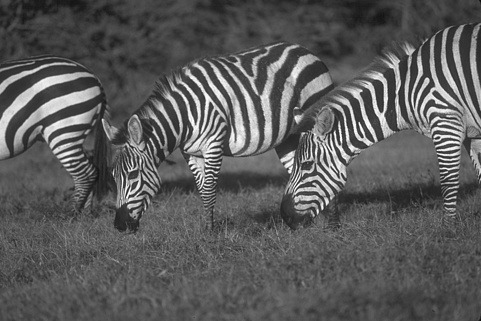
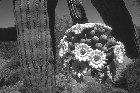
Original image $t=2\cdot 10^{-6}$ Steady state (46)

Figure 5: Global contrast enhancement using $\varPhi=\varPhi_{1,1}$ and greyscale versions of images from the BSDS500 [2].

As a first option one can use the explicit scheme (50) to describe the evolution of all grey values $v_{i}$ up to some time $t$ (see column two of Figure 5). The amount of contrast enhancement grows with increasing values of $t$. In our experiments an image size of $481\times 321$ pixels and the application of the flux function $\varPhi_{1,1}$ with $L_{\varPhi}=1$ imply an upper bound of $1/(2\cdot 481\cdot 321)$ for $\tau$. Thus, we can achieve the time $t=2\cdot 10^{-6}$ in Figure 5 in a single iteration. If one is only interested in an enhanced version of the original image with maximum global contrast there is an alternative, namely the derived steady state solution for linear flux functions (46). The results are shown in the last column of Figure 5. This figure also confirms that the solution of the explicit scheme (50) converges to the steady-state solution (46) for $t\to\infty$. From (46) it is clear that this steady state is equivalent to histogram equalisation. In summary, this means that the application of our global model to greyscale images offers an evolution equation histogram equalisation which allows to control the amount of contrast enhancement in an intuitive way through the time parameter $t$.

5.1.2 Local Contrast Enhancement

In order to achieve local contrast enhancement we use our model to describe the evolution of grey values $v_{i}$ at all $n_{x}\cdot n_{y}$ image grid positions. The change of every grey value $v_{i}$ depends on all grey values within a disk-shaped neighbourhood of radius $\varrho$ around its grid position $\bm{x}_{i}$. We assume that

$$\tilde{w}_{i,j}:=\gamma(|\bm{x}_{j}-\bm{x}_{i}|),\qquad\forall i,j\in\{1,2,\ldots,N\},$$ (69)

where we weight the spatial distance $|\bm{x}_{j}-\bm{x}_{i}|$ by a function $\gamma:\mathbb{R}_{0}^{+}\to[0,1]$ with compact support $[0,\varrho)$ which fulfils

$$\gamma(x)\in(0,1], \text{if }x<\varrho,$$ (70)

$$\gamma(x)=0, \text{if }x\geq\varrho.$$

The choice of $\gamma$ is application dependent. However, it usually makes sense to define $\gamma(x)$ as a non-increasing function in $x$. Possible choices are e.g.

$$\gamma_{1}(x) =\begin{cases}1,&\text{if }x<\varrho,\\ 0,&\text{else},\end{cases}$$ (71)

$$\gamma_{2}(x) =\begin{cases}1-6\frac{x^{2}}{\varrho^{2}}+6\frac{x^{3}}{\varrho^{3}},&\text{if }0\leq x<\frac{\varrho}{2},\\ 2\cdot(1-\frac{x}{\varrho})^{3},&\text{if }\frac{\varrho}{2}\leq x<\varrho,\\ 0,&\text{else},\end{cases}$$ (72)

which are both sketched in Figure 6.

Figure 6: Box function $\gamma_{1}$ and scaled cubic B-spline $\gamma_{2}$.

When applying this local model to images we make use of mirroring boundary conditions in order to avoid artefacts at the image boundaries. Figure 7 provides an example for local contrast enhancement of digital greyscale images.

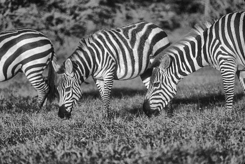
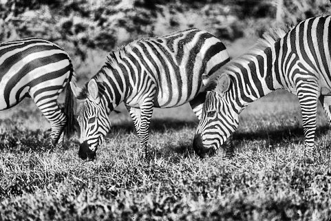
Original image $t=2\cdot 10^{-5}$ $t=4\cdot 10^{-5}$

Figure 7: Local contrast enhancement using $\varPhi=\varPhi_{1,1}$, $\gamma=\gamma_{1}$, $\varrho=60$, and greyscale versions of images from the BSDS500 [2].

Again, we describe the grey value evolution with the explicit scheme (50). Furthermore, we use $\gamma_{1}$ to model the influence of neighbouring grey values. As is evident from Figure 7, increasing the values for $t$ goes along with enhanced local contrast.

5.2 Colour Images

Based on the assumption that our input data is given in sRGB colour space [48] (in the following denoted by RGB) we represent a digital colour image by the mapping $f:\{1,\ldots,n_{x}\}\times\{1,\ldots,n_{y}\}\to[0,1]^{3}$. Subsequently, our aim is the contrast enhancement of digital colour images without distorting the colour information. This means that we only want to adapt the luminance but not the chromaticity of a given image. For this purpose, we convert the given image data to YCbCr colour space [44, Section 3.5] since this representation provides a separate luminance channel. Next, we perform contrast enhancement on the luminance channel only. Just as for greyscale images we map all Y-values to the interval $(0,1)$ to fulfil our model requirements. After enhancing the contrast, we transform the colour information of the image back to RGB colour space.

At this point it is important to mention that the colour gamut of the RGB colour space is a subset of the YCbCr colour gamut and during the conversion process of colour coordinates from YCbCr to RGB colour space the so-called colour gamut problem may occur: Colours from the YCbCr colour gamut may lie outside the RGB colour gamut and thus cannot be represented in RGB colour coordinates. Naik and Murthy [32] state that a simple clipping of the values to the bounds creates undesired shift of hue and may lead to colour artefacts. In order to avoid the colour gamut problem we adapt the ideas presented by Nikolova and Steidl [34] which are based on the intensity representation of the HSI colour space [20, Section 6.2.3]. Using the original and enhanced intensities, they define an affine colour mapping and transform the original RGB values. This preserves the hue and results in an enhanced RGB image. It is straightforward to show that their algorithms are valid for any intensity $\hat{f}$ of type

$$\hat{f}=c_{r}\cdot r+c_{g}\cdot g+c_{b}\cdot b,$$ (73)

with $c_{r}+c_{g}+c_{b}=1$ and $c_{r},c_{g},c_{b}\in[0,1]$, where $r$, $g$, and $b$ denote RGB colour coordinates. Thus, they are applicable to the luminance representation of the YCbCr colour space, too, i.e. $c_{r}=0.299$, $c_{g}=0.587$, $c_{b}=0.114$. Tian and Cohen make use of the same idea in [52]. As in [34], our result image is a convex combination of the outcomes of a multiplicative and an additive algorithm (see [34, Algorithm 4 and 5]) with coefficients $\lambda$ and $1-\lambda$ for $\lambda\in[0,1]$. During our experiments we use a fixed value of $\lambda=0.5$ (for details on how to choose $\lambda$ we refer to [34]). An overview of our strategy for contrast enhancement of digital colour value images is given in Figure 8.

Figure 8: Procedure of contrast enhancement for digital colour images following [34].

5.2.1 Global Contrast Enhancement

Again, we apply the global model from Section 3.2 in order to achieve global contrast enhancement. As mentioned before, we consider the $N$ different occurring Y-values of the YCbCr representation of the input image and denote them by $v_{i}$ (similar to Section 5.1.1 we neglect their positions in the image). Every entry of the weighting matrix $\tilde{w}_{i,j}$ contains the number of occurences of the value $v_{j}$ in the Y-channel of the image. It becomes clear that the application of our model – in this setting – basically comes down to histogram equalisation of the Y-channel. Figure 9 shows the resulting RGB images after global contrast enhancement. Similar to the greyscale scenario, we can either apply the explicit scheme (50) or – for $\varPhi=\varPhi_{a,1}$ – estimate the steady state solution following (46). For the first case the amount of contrast enhancement grows with the positive time parameter $t$. The second column of Figure 9 shows the results for $\varPhi=\varPhi_{1,1}$ given time $t$. The corresponding steady state solutions are illustrated in the last column of Figure 9.

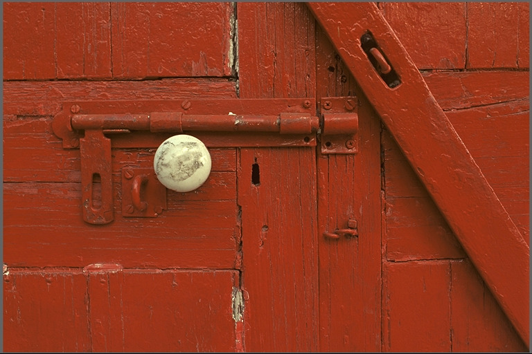
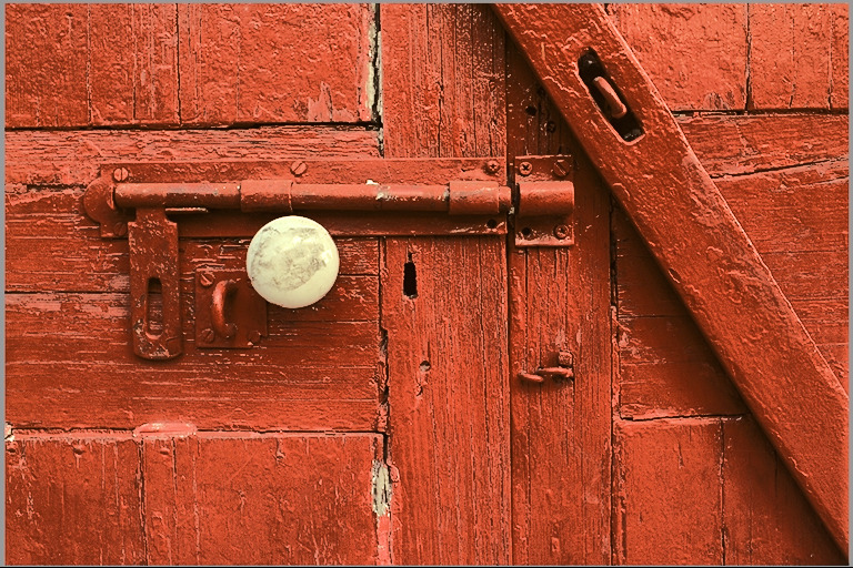
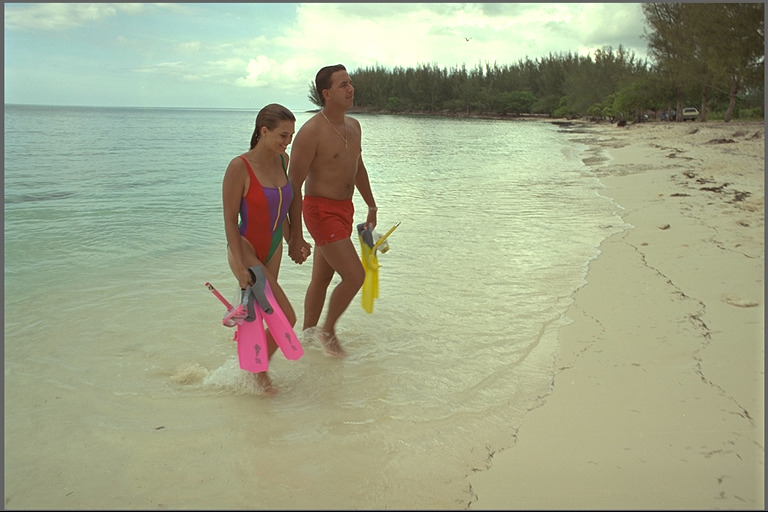
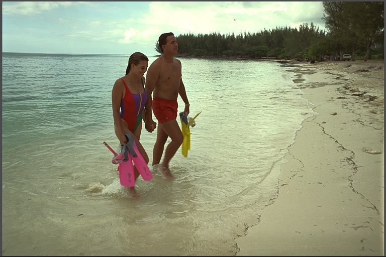
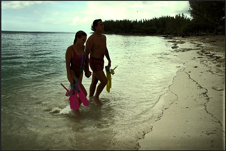
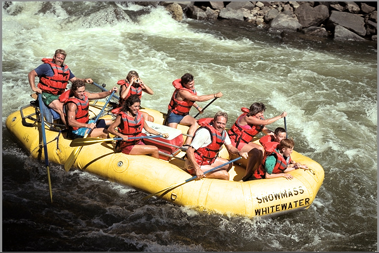
Original image $t=5\cdot 10^{-7}$ Steady state (46)

Figure 9: Global contrast enhancement using $\varPhi=\varPhi_{1,1}$, $\lambda=0.5$, and images from [1].

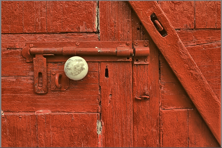
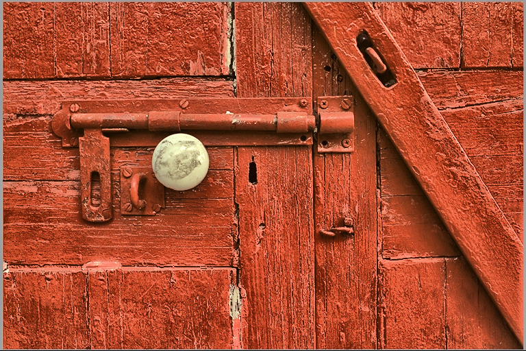
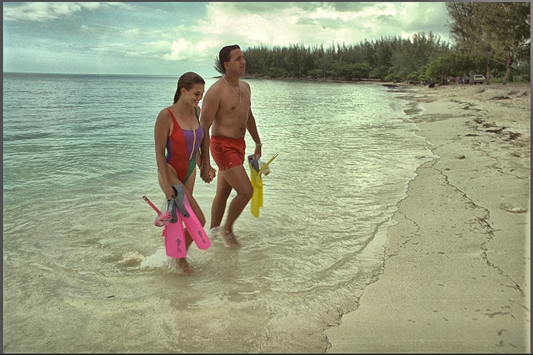
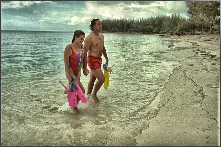
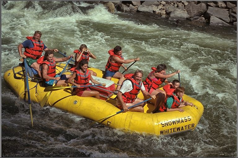
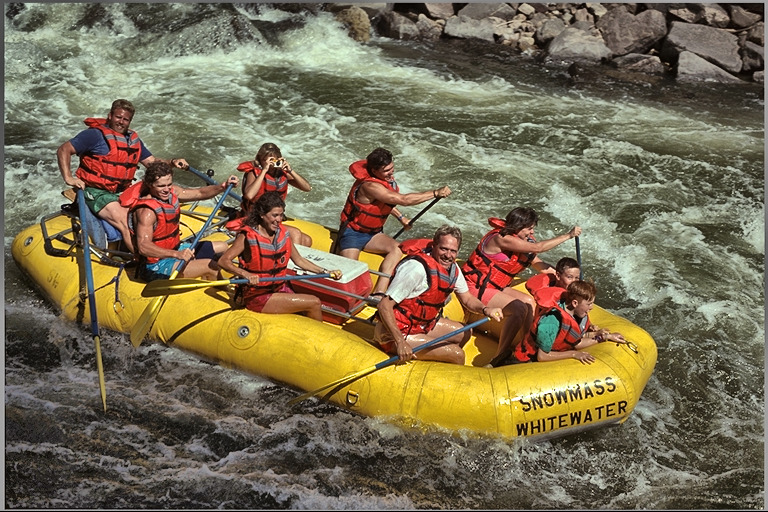
Original image $t=1\cdot 10^{-5}$ $t=2\cdot 10^{-5}$

Figure 10: Local contrast enhancement using $\varPhi=\varPhi_{1,1}$, $\gamma=\gamma_{1}$, $\varrho=60$, $\lambda=0.5$, and images from [1].

5.2.2 Local Contrast Enhancement

In a similar manner – and adapting the ideas from Subsection 5.1.2 – we achieve local contrast enhancement in colour images. For this purpose we describe the evolution of Y-values $v_{i}$ at all $n_{x}\cdot n_{y}$ image grid positions using a disk-shaped neighbourhood of radius $\varrho$ around the corresponding grid positions $\bm{x}_{i}$. The entries of the weighting matrix $\bm{\tilde{W}}$ follow (69). In combination with mirrored boundary conditions the explicit scheme (50) allows to increase the local contrast of an image with growing $t$. Figure 10 shows exemplary results for $\varPhi=\varPhi_{1,1}$ and $\gamma=\gamma_{1}$ (cf. (71)). Note, how well – in comparison to the global set-up in Figure 9 – the structure of the door gets enhanced while the details of the door knob are preserved. The differences are even larger in the second image: For both the couple in the foreground and the background scenery, contrast increases which implies visibility also for larger times $t$.

5.3 Parameters

In total, our model has up to six parameters: $\varPhi$, $\tau$, $t$, $\lambda$, $\varrho$, and $\gamma$. During our experiments we have fixed $\varPhi(s)$ to the linear flux function $\varPhi_{1,1}(s)$ and $\lambda$ to $0.5$. Valid bounds for the time step size $\tau$ are given in Theorems 4.1–4.3. From the theory in Section 3 and the subsequent experiments on greyscale and colour images it becomes clear that the amount of contrast enhancement grows with the diffusion time. Thus, it remains to discuss the influence of the parameters $\varrho$ and $\gamma$. We found out that the neighbourhood radius $\varrho$ affects the diffusion time and controls the amount of perceived local contrast enhancement, i.e. it steers the localisation of the contrast enhancement process. Whereas small radii lead to high contrast in already small image areas, the size of image sections with high contrast increases with $\varrho$. For sufficiently large values of $\varrho$ global histogram equalisation is approximated. Another interesting point is the choice of the weighting function $\gamma$. Overall, choosing $\gamma=\gamma_{1}$ leads to more homogeneous contrast enhancement resulting in smoother perception. For $\gamma=\gamma_{2}$ the focus always lies on the neighbourhood centre which implies even more enhancement of local structures than in the preceding case. In summary, $\gamma_{2}$ leads to more enhancement which, however, also creates undesired effects in smooth or noisy regions. Thus, we prefer $\gamma_{1}$ over $\gamma_{2}$. Further experiments which visualise the effect of the parameters can be found in the supplementary material.

5.4 Related Work from an Application Perspective

Now that we have demonstrated the applicability of our model to digital images we want to discuss briefly its relation to other existing theories in the context of image processing.

As mentioned in Section 5.1.1, applying the global model – with the entries of $\bm{\tilde{W}}$ representing the grey value frequencies – is identical to histogram equalisation (a common formulation can e.g. be found in [20]). Furthermore, there exist other closely related histogram specification techniques – such as [45, 35, 36] – which can have the same steady state. If we compare our evolution with the histogram modification flow introduced by Sapiro and Caselles [45], we see that their flow can also be translated into a combination of repulsion among grey-values and a barrier function. However, in [45] the repulsive force is constant, and the barrier function quadratic. Thus, they cannot be derived from the same kind of interaction between the $v_{i}$ and their reflected counterparts as in our paper.

Referring to Section 5.1.2, there also exist well-known approaches which aim to enhance the local image contrast such as adaptive histogram equalisation – see [42] and the references therein – or contrast limited adaptive histogram equalisation [56]. The latter technique tries to overcome the over-amplification of noise in mostly homogeneous image regions when using adaptive histogram equalisation. Both approaches share the basic idea with our approach in Section 5.1.2 and perform histogram equalisation for each pixel, i.e. the mapping function for every pixel is determined using a neighbourhood of predefined size and its corresponding histogram.

Another related research topic is the rich field of colour image enhancement which we broach in Section 5.2. A short review of existing methods – as well as two new ideas – is presented in [3]. Therein, Bassiou and Kotropoulus also mention the colour gamut problem for methods which perform contrast enhancement in a different colour space and transform colour coordinates to RGB afterwards. Of particular interest are the publications by Naik and Murthy [32] and Nikolova and Steidl [34] whose ideas are used in Section 5.2. Both of them suggest – based on an affine colour transform – strategies to overcome the colour gamut problem while avoiding colour artefacts in the resulting image. A recent approach which also makes use of these ideas is presented by Tian and Cohen [52]. Ojo et al. [37] make use of the HSV colour space to avoid the colour gamut problem when enhancing the contrast of colour images. A variational approach for contrast enhancement which tries to approximate the hue of the input image was recently published by Pierre et al. [41].

6 Conclusions and Outlook

In our paper we have presented a mathematical model which describes pure backward diffusion as gradient descent of strictly convex energies. The underlying evolution makes use of ideas from the area of collective behaviour and – in terms of the latter – our model can be understood as a fully repulsive discrete first order swarm model. Not only it is surprising that our model allows backward diffusion to be formulated as a convex optimisation problem but also that it is sufficient to impose reflecting boundary conditions in the diffusion co-domain in order to guarantee stability. This strategy is contrary to existing approaches which either assume forward or zero diffusion at extrema or add classical fidelity terms to avoid instabilities. Furthermore, discretisation of our model does not require sophisticated numerics. We have proven that a straightforward explicit scheme is sufficient to preserve the stability of the time-continuous evolution. In our experiments, we show that our model can directly be applied to contrast enhancement of digital greyscale and colour images.

We see our contribution mainly as an example of stable modelling of backward parabolic evolutions that create neither theoretical nor numerical problems. We are convinced that this concept has far more widespread applications in inverse problems, image processing, and computer vision. Exploring them will be part of our future research.

Acknowledgements

Our research on intrinsic stability properties of specific backward diffusion processes goes back to 2005, when Joachim Weickert was visiting Mila Nikolova in Paris. Unfortunately the diffusion equation considered at that time did not have the expected properties, such that it took one more decade to come up with more appropriate models. Leif Bergerhoff wishes to thank Antoine Gautier and Peter Ochs for fruitful discussions around the topic of the paper. This project has received funding from the DFG Cluster of Excellence Multimodal Computing and Interaction and from the European Union’s Horizon 2020 research and innovation programme (grant agreement No 741215, ERC Advanced Grant INCOVID). This is gratefully acknowledged.

References

- [1] Kodak Lossless True Color Image Suite. http://www.r0k.us/graphics/kodak/, last visited August 31, 2018
- [2] Arbelaez, P., Maire, M., Fowlkes, C., Malik, J.: Contour detection and hierarchical image segmentation. IEEE Transactions on Pattern Analysis and Machine Intelligence 33(5), 898–916 (2011)
- [3] Bassiou, N., Kotropoulos, C.: Color image histogram equalization by absolute discounting back-off. Computer Vision and Image Understanding 107(1), 108–122 (Jul 2007)
- [4] Bergerhoff, L., Cárdenas, M., Weickert, J., Welk, M.: Modelling stable backward diffusion and repulsive swarms with convex energies and range constraints. In: Pelillo, M., Hancock, E. (eds.) Energy Minimization Methods in Computer Vision and Pattern Recognition, 11th International Conference, EMMCVPR 2017, Venice, Italy. Lecture Notes in Computer Science, vol. 10746, pp. 409–423. Springer, Cham (Mar 2018)
- [5] Bergerhoff, L., Weickert, J.: Modelling image processing with discrete first-order swarms. In: Pillay, N., Engelbrecht, P.A., Abraham, A., du Plessis, C.M., Snášel, V., Muda, K.A. (eds.) Advances in Nature and Biologically Inspired Computing, vol. 419, pp. 261–270. Springer, Cham (2016)
- [6] Carasso, A., Sanderson, J., Hyman, J.: Digital removal of random media image degradations by solving the diffusion equation backwards in time. SIAM Journal on Numerical Analysis 15(2), 344–367 (Apr 1978)
- [7] Carasso, A.S.: Compensating operators and stable backward in time marching in nonlinear parabolic equations. GEM - International Journal on Geomathematics 5(1), 1–16 (Apr 2014)
- [8] Carasso, A.S.: Stable explicit time marching in well-posed or ill-posed nonlinear parabolic equations. Inverse Problems in Science and Engineering 24(8), 1364–1384 (2016)
- [9] Carasso, A.S.: Stabilized Richardson leapfrog scheme in explicit stepwise computation of forward or backward nonlinear parabolic equations. Inverse Problems in Science and Engineering 25(12), 1719–1742 (2017)
- [10] Carrillo, J.A., Fornasier, M., Toscani, G., Vecil, F.: Particle, kinetic, and hydrodynamic models of swarming. In: Naldi, G., Pareschi, L., Toscani, G. (eds.) Mathematical Modeling of Collective Behavior in Socio-Economic and Life Sciences, pp. 297–336. Birkhäuser, Boston (2010)
- [11] Chuang, Y.L., Huang, Y.R., D’Orsogna, M.R., Bertozzi, A.L.: Multi-vehicle flocking: Scalability of cooperative control algorithms using pairwise potentials. In: 2007 IEEE International Conference on Robotics and Automation, ICRA 2007, 10-14 April 2007, Roma, Italy. pp. 2292–2299 (2007)
- [12] D’Orsogna, M.R., Chuang, Y.L., Bertozzi, A.L., Chayes, L.S.: Self-propelled particles with soft-core interactions: Patterns, stability, and collapse. Physical Review Letters 96, 104302 (Mar 2006)
- [13] Fu, C.L., Xiong, X.T., Qian, Z.: Fourier regularization for a backward heat equation. Journal of Mathematical Analysis and Applications 331(1), 472–480 (2007)
- [14] Gabor, D.: Information theory in electron microscopy. Laboratory Investigation 14, 801–807 (Jun 1965)
- [15] Gazi, V., Fidan, B.: Coordination and control of multi-agent dynamic systems: Models and approaches. In: Sahin, E., Spears, W.M., Winfield, A.F.T. (eds.) Swarm Robotics, Lecture Notes in Computer Science, vol. 4433, pp. 71–102. Springer, Berlin (2007)
- [16] Gazi, V., Passino, K.M.: Stability analysis of swarms. IEEE Transactions on Automatic Control 48(4), 692–697 (Apr 2003)
- [17] Gazi, V., Passino, K.M.: Stability analysis of social foraging swarms. IEEE Transactions on Systems, Man, and Cybernetics, Part B: Cybernetics 34(1), 539–557 (Feb 2004)
- [18] Gerschgorin, S.: Über die Abgrenzung der Eigenwerte einer Matrix. Bulletin de l’Académie des Sciences de l’URSS. Classe des sciences mathématiques et naturelles pp. 749–754 (1931)
- [19] Gilboa, G., Sochen, N.A., Zeevi, Y.Y.: Forward-and-backward diffusion processes for adaptive image enhancement and denoising. IEEE Transactions on Image Processing 11(7), 689–703 (2002)
- [20] Gonzalez, R., Woods, R.: Digital Image Processing. Prentice-Hall, Upper Saddle River, NJ, USA, third edn. (2008)
- [21] Gronwall, T.H.: Note on the derivatives with respect to a parameter of the solutions of a system of differential equations. Annals of Mathematics 20(4), 292–296 (Jul 1919)
- [22] Hadamard, J.: Sur les problèmes aux dérivées partielles et leur signification physique. Princeton University Bulletin 13, 49–52 (1902)
- [23] Hào, D.N., Duc, N.V.: Stability results for the heat equation backward in time. Journal of Mathematical Analysis and Applications 353(2), 627–641 (May 2009)
- [24] Hào, D.N., Duc, N.V.: Stability results for backward parabolic equations with time-dependent coefficients. Inverse Problems 27(2), 025003 (Jan 2011)
- [25] Hummel, R.A., Kimia, B.B., Zucker, S.W.: Deblurring Gaussian blur. Computer Vision, Graphics, and Image Processing 38(1), 66–80 (Apr 1987)
- [26] John, F.: Numerical solution of the equation of heat conduction for preceding times. Annali di Matematica Pura ed Applicata 40(1), 129–142 (Dec 1955)
- [27] Kirkup, S., Wadsworth, M.: Solution of inverse diffusion problems by operator-splitting methods. Applied Mathematical Modelling 26(10), 1003–1018 (2002)
- [28] Kovásznay, L.S.G., Joseph, H.M.: Image processing. Proceedings of the IRE 43(5), 560–570 (May 1955)
- [29] Lindenbaum, M., Fischer, M., Bruckstein, A.M.: On Gabor’s contribution to image enhancement. Pattern Recognition 27(1), 1–8 (Jan 1994)
- [30] Lyapunov, A.M.: The general problem of the stability of motion. International Journal of Control 55(3), 531–534 (1992)
- [31] Mair, B.A., Wilson, D.C., Reti, Z.: Deblurring the discrete Gaussian blur. In: Proceedings of the Workshop on Mathematical Methods in Biomedical Image Analysis. pp. 273–277. IEEE, Los Alamitos (Jun 1996)
- [32] Naik, S.K., Murthy, C.A.: Hue-preserving color image enhancement without gamut problem. IEEE Transactions on Image Processing 12(12), 1591–1598 (Dec 2003)
- [33] Nesterov, Y.: Introductory Lectures On Convex Optimization. Springer, New York (2004)
- [34] Nikolova, M., Steidl, G.: Fast hue and range preserving histogram specification: Theory and new algorithms for color image enhancement. IEEE Transactions on Image Processing 23(9), 4087–4100 (Sep 2014)
- [35] Nikolova, M., Steidl, G.: Fast ordering algorithm for exact histogram specification. IEEE Transactions on Image Processing 23(12), 5274–5283 (Dec 2014)
- [36] Nikolova, M., Wen, Y.W., Chan, R.: Exact histogram specification for digital images using a variational approach. Journal of Mathematical Imaging and Vision 46(3), 309–325 (Jul 2013)
- [37] Ojo, J.A., Solomon, I.D., Adeniran, S.A.: Colour-preserving contrast enhancement algorithm for images. In: Chen, L., Kapoor, S., Bhatia, R. (eds.) Emerging Trends and Advanced Technologies for Computational Intelligence: Extended and Selected Results from the Science and Information Conference 2015. pp. 207–222. Springer, Cham (2016)
- [38] Osher, S., Rudin, L.: Shocks and other nonlinear filtering applied to image processing. In: Tescher, A.G. (ed.) Applications of Digital Image Processing XIV, Proceedings of SPIE, vol. 1567, pp. 414–431. SPIE Press, Bellingham (1991)
- [39] Perko, L.: Differential Equations and Dynamical Systems. No. 7 in Texts in Applied Mathematics, Springer, third edn. (2001)
- [40] Perona, P., Malik, J.: Scale space and edge detection using anisotropic diffusion. IEEE Transactions on Pattern Analysis and Machine Intelligence 12, 629–639 (1990)
- [41] Pierre, F., Aujol, J.F., Bugeau, A., Steidl, G., Ta, V.T.: Variational contrast enhancement of gray-scale and RGB images. Journal of Mathematical Imaging and Vision 57(1), 99–116 (Jan 2017)
- [42] Pizer, S.M., Amburn, E.P., Austin, J.D., Cromartie, R., Geselowitz, A., Greer, T., ter Haar Romeny, B.M., Zimmerman, J.B., Zuiderveld, K.: Adaptive histogram equalization and its variations. Computer Vision, Graphics, and Image Processing 39(3), 355–368 (1987)
- [43] Pollak, I., Willsky, A.S., Krim, H.: Image segmentation and edge enhancement with stabilized inverse diffusion equations. IEEE Transactions on Image Processing 9(2), 256–266 (Feb 2000)
- [44] Pratt, W.K.: Digital Image Processing. Wiley & Sons, New York, third edn. (2001)
- [45] Sapiro, G., Caselles, V.: Histogram modification via differential equations. Journal of Differential Equations 135, 238–268 (1997)
- [46] Sochen, N.A., Zeevi, Y.Y.: Resolution enhancement of colored images by inverse diffusion processes. In: Proc. 1998 IEEE International Conference on Acoustics, Speech and Signal Processing. pp. 2853–2856. Seattle, WA (May 1998)
- [47] Steiner, A., Kimmel, R., Bruckstein, A.M.: Planar shape enhancement and exaggeration. Graphical Models and Image Processing 60(2), 112–124 (Mar 1998)
- [48] Stokes, M., Anderson, M., Chandrasekar, S., Motta, R.: A standard default color space for the internet - sRGB (version 1.10). https://www.w3.org/Graphics/Color/sRGB (Nov 1996), last visited August 31, 2018
- [49] Tautenhahn, U., Schröter, T.: On optimal regularization methods for the backward heat equation. Zeitschrift für Analysis und ihre Anwendungen 15(2), 475–493 (1996)
- [50] ter Haar Romeny, B.M., Florack, L.M.J., de Swart, M., Wilting, J., Viergever, M.A.: Deblurring Gaussian blur. In: Bookstein, F.L., Duncan, J.S., Lange, N., Wilson, D.C. (eds.) Mathematical Methods in Medical Imaging III, Proceedings of SPIE, vol. 2299, pp. 139–148. SPIE Press, Bellingham (Jul 1994)
- [51] Ternat, F., Orellana, O., Daripa, P.: Two stable methods with numerical experiments for solving the backward heat equation. Applied Numerical Mathematics 61(2), 266–284 (Feb 2011)
- [52] Tian, Q.C., Cohen, L.D.: Color consistency for photo collections without gamut problems. In: Amsaleg, L., Guðmundsson, G., Gurrin, C., Jónsson, B., Satoh, S. (eds.) MultiMedia Modeling: 23rd International Conference, MMM 2017, Reykjavik, Iceland, January 4-6, 2017, Proceedings, Part I. pp. 90–101. Springer, Cham (Jan 2017)
- [53] Welk, M., Gilboa, G., Weickert, J.: Theoretical foundations for discrete forward-and-backward diffusion filtering. In: Tai, X.C., Mørken, K., Lysaker, M., Lie, K.A. (eds.) Scale Space and Variational Methods in Computer Vision, Lecture Notes in Computer Science, vol. 5567, pp. 527–538. Springer, Berlin (2009)
- [54] Welk, M., Weickert, J., Gilboa, G.: A discrete theory and efficient algorithms for forward-and-backward diffusion filtering. Journal of Mathematical Imaging and Vision 60(9), 1399–1426 (Nov 2018)
- [55] Zhao, Z., Meng, Z.: A modified Tikhonov regularization method for a backward heat equation. Inverse Problems in Science and Engineering 19(8), 1175–1182 (2011)
- [56] Zuiderveld, K.: Contrast Limited Adaptive Histogram Equalization. In: Heckbert, P.S. (ed.) Graphics Gems IV, pp. 474–485. Academic Press Professional, Inc., San Diego, CA, USA (1994)