Inferring the covariant $\Theta$-exact noncommutative coupling in the top quark pair production at linear colliders

Abstract

A novel non-minimal interaction of neutral right-handed fermion and abelian gauge field in the covariant $\Theta$-exact noncommutative standard model (NCSM) which is invariant under Very Special Relativity (VSR) Lorentz subgroup, opens an avenue to study the top quark pair production at linear colliders. Here the non-minimal coupling is denoted as $\kappa$ and the noncommutative (NC) scale $\Lambda$. In this work, we consider two types of analysis, one is without considering helicity basis technique and another, considering helicity of the initial and final state particles. Further, the realistic electron and positron beam polarization are taken into account to measure the NC parameters. In the first case, when $\kappa$ is positive and certain values of $\Lambda$, we found that a specific threshold value of machine energy (optimal energy in the units of GeV) $\sqrt{s_{0}}$ ($\simeq 2.52~{}\Lambda+39$ ) may be quite useful to look for the signature of the spacetime noncommutativity with unpolarized beam. The statistical $\chi^{2}$ analysis of the azimuthal anisotropy which is due to broken rotational invariance about the beam axis, is quite possible when $\kappa$ takes negative value $0>\kappa>-0.596$ which persuade a lower limit on NC scale $\Lambda$ ($1.0\,\text{to}\,2.4\,\text{TeV}$) at $\kappa_{max}=-0.296$ with $95\%$ C.L according to luminosity ranging from $100\,fb^{-1}\text{to}1000\,fb^{-1}$ at machine energy $\sqrt{s}=1.4\,\text{TeV}\,\text{and}\,3.0\,\text{TeV}$. In another case, we perform detailed analysis for the polarized and unpolarized electron-positron beam to probe spacetime noncommutativity in light of following observables like azimuthal anisotropy, helicity correlation, and top quark helicity left-right asymmetry. The polarization of the initial beam $\{P_{e^{-}},P_{e^{+}}\}=\{-0.8,0.3\}(\{-0.8,0.6\})$ enhances the ranges of lower limit on $\Lambda$, $i.e.\,1.13\,\text{to}\,2.80\,\text{TeV}$ at $\kappa_{max}$ alongside the $\kappa_{max}$ enhanced into $-0.5445\,(-0.607)$ $95\%$C.L accord with luminosity and machine energy. Finally, we studied the intriguing mixing of the UV and the IR by invoking a specific structure of noncommutative anti-symmetric tensor $\Theta_{\mu\nu}$ which is invariant under translational $T(2)$ VSR Lorentz subgroup.

1 Introduction

After the discovery of the Higgs boson (the only missing link of the standard model) at the Large Hadron Collider (LHC) at CERN, the Standard Model (SM) of Particle Physics, despite its inability of explaining the higgs hierarchy problem, neutrino mass problem, baryon asymmetry etc, is now widely believed to be a low energy effective field theory. Now if there is physics beyond the standard model (BSM), it is expected to show up at the TeV energy colliders i.e. at the LHC or at the upcoming electron-positron Linear Collider. Among the class of BSM models, supersymmetry, extra dimension, space-time noncommutativity are found to be quite interesting because of their rich phenomenological content. A host of phenomenological investigations have already been made and are available in the literature.

The gravity which becomes strong at the TeV energy scale in large extra dimensional model ADD ; AADD , makes the spacetime noncommutative (i.e. fuzzy) at the TeV scale. The signature of the TeV scale spacetime noncommutativity can be found at the TeV energy electron-positron linear collider or hadron colliders. Snyder’s pioneering work Snyder and the recent advancement in low energy string theory manifests the fact that spacetime can be noncommutative CDS ; DH ; SW ; SST and it has generated a lot of enthusiasm about the TeV scale spacetime noncommutativity among the particle physics community. In 1996, Witten et.al., Witten ; HW has suggested that one can probe the stringy effects by lowering the threshold value of noncommutativity to TeV, a scale which is not so far from present or future collider energy scale.

Now at high energy when gravity becomes strong, the spacetime coordinates become an operator $\hat{x}_{\mu}$. They no longer commute, satisfying the algebra

$$[\hat{x}_{\mu},\hat{x}_{\nu}]=i\Theta_{\mu\nu}=\frac{ic_{\mu\nu}}{\Lambda^{2}}$$ (1)

Here $\Theta_{\mu\nu}$ (of mass dimension $-2$) is real and antisymmetric tensor. $c_{\mu\nu}$ is the antisymmetric constant and $\Lambda$, the noncommutative scale. In the noncommutative space, the ordinary product between fields is replaced by Moyal-Weyl(MW) DN ; RJ ; JS star($\star$) product defined by

$$(f\star g)(x)=exp\left(\frac{i}{2}\Theta_{\mu\nu}\partial_{x^{\mu}}\partial_{y^{\nu}}\right)f(x)g(y)|_{y=x}.$$ (2)

In the theoretical point of view, it is expected that the spacetime noncommutative (NC) field theories should reduce into a commutative field theory when $\Theta\rightarrow 0$ or whenever the momenta of the field quanta are much smaller than $1/\sqrt{|\Theta|}$. Although such naive expectation is valid at tree level interaction but it suffers by infamous UV/IR mixing phenomenon at the loop level which is shown by Filk and Minwalla in filk ; YMNC1 ; Minwalla ; IRseiberg1 respectively. The UV/IR mixing arises due to non-planar Feynman diagram at loop level, precisely due to Moyal phase. But in the NC gauge theory, the expansion of Moyal star product between fields breaks the invariance of the truncated action. Seiberg and Witten SW formulated a map as a power series of $\Theta$ which relates the NC gauge theory and commutative gauge theory, thereby the NC action is gauge invariant at any order $\Theta$. There are two types of map which are, the expansion of $\Theta$ with keeping gauge field all order and the expansion of gauge field with keeping $\Theta$ all order namely $\Theta$-expanded and $\Theta$-exact Seiberg-Witten map (SW map) respectively. The $\Theta$-expanded SW map for matter field $\psi$, gauge field $A^{\mu}$ are written as a power series of the noncommutative parameter $\Theta$ as follows DH ; SW ; Witten ; HW ; DN ; RJ ; JS

$$\widehat{\psi}(x,\Theta) = \psi(x)+\Theta\psi^{(1)}+\Theta^{2}\psi^{(2)}+\cdots$$ (3)

$$\widehat{A}_{\mu}(x,\Theta) = A_{\mu}(x)+\Theta A_{\mu}^{(1)}+\Theta^{2}A_{\mu}^{(2)}+\cdots$$ (4)

The second order ($e^{2}$), third order($e^{3}$) and further expansions of $\Theta$-exact SW maps are rather complicated than $\Theta$-expanded SW map construction due to gauge structure degrees of freedom Trampetic3 . In the $\Theta$-expanded approach, the NC theory is renormalizable in linear order at one-loop level Minwalla . In the $\Theta$-exact SW map approach, the UV/IR mixing is related to phase factor of distinctive star product between commutative fields. The phenomenological implications of the $\Theta$-exact SW map and properties of UV/IR mixing pursued extensively in ref Trampetic4 ; Martin1 . There are enormous amount of work has been done considering Moyal-Weyl (MW) approach Minwalla ; MWURIR1 ; MWURIR2 ; MWURIR3 ; MWURIR4 ; MWURIR5 ; MWURIR6 as well as Seiberg-Witten Map approach SWURIR1 ; SWURIR2 ; SWURIR3 ; SWURIR4 ; SWURIR5 ; SWURIR6 ; SWURIR7 ; SWURIR8 ; SWURIR9 ; HKT3 in order to remove the UV/IR mixing. The role of supersymmetric Yang-Mills theory in the noncommutative UV/IR mixing petrov1 ; petrov2 ; Trampetic1 ; Trampetic2 ; ABJM were extensively scrutinized to overcome the divergences which appeared in the field non-local interaction. Other class of NC theories namely, non-geometric theories like $\kappa$-Minkowski spacetime and Snyder spacetime also exhibits the UV/IR mixing at one-loop level kappa1 ; Snyder1 ; Snyder2 . In general, the UV/IR mixing is the universal property of all NCQFT. But in the ref kappa2 , it is shown that the truncated $\kappa$-deformed action does not possess the UV/IR mixing due to implementation of the $\kappa$-deformed star products in the $\kappa$-Minkowski spacetime which evades the integral measure problems. On the contrary, in the Snyder-type star product in the Snyder spacetime, the $\phi^{4}$ interaction breaks the translational invariance as well as it celebrates the UV/IR mixing at the one-loop tadpole contribution to the two-point function Snyder1 ; Snyder2 . The non-associativity induces such UV/IR mixing in the Synder NC scalar field theory in both momentum-conserving as well as momentum-nonconserving approach. Moreover notwithstanding the UV/IR mixing, the covariant $\Theta$-exact NC theory HKT1 has cosmological implications on the decoupling/coupling temperature of right-handed neutrino at the early universe ptolemy1 ; ptolemy2 ; astro2020 as well as primordial nucleosynthesis HT and ultra high energy (UHE) cosmic ray experiments HKT2 .

In the phenomenological point of view, based on the MW approach, the Moller scattering, Bhabha scattering and electron-photon scattering were first studied in ref HPR ; Hewett . The processes $\gamma\gamma\to e^{+}e^{-}$ and $\gamma\gamma\to\gamma\gamma$ were investigated in Mathews ; Rizzo . A review on NC phenomenology is available here HKM . A lot of NC phenomenology using the Seiberg-Witten technique is available. Calmet et.al., CJSWW ; CW first constructed the standard model in the noncommutative spacetime, which is the minimal version of the Noncommutative Standard Model (mNCSM). There exists another version, called non-minimal version of NCSM i.e. nmNCSM Melic in which besides the usual mNCSM interaction vertices, a host of new vertices e.g. triple neutral gauge boson vertices also arises which are found to be absent in the mNCSM and of course in the SM. These new vertices lead to several interesting decays e.g. $Z\to\gamma\gamma,~{}gg$ which are forbidden in the SM. These were studied in BDDSTW ; AJSW ; DST ; BLRT1 ; EH1 . In the SW map approach, ref AOR first investigated the neutral vector boson ($\gamma$, $z$) pair production in the noncommutative spacetime at the LHC and they obtained the bound on the noncommutative scale $\Lambda\geq 1~{}\rm{TeV}$. The $W^{\pm}$ pair production Ohl also studied and found that the azimuthal distribution is oscillatory corresponding to $\Lambda_{NC}=0.7~{}\rm{TeV}$, which differs significantly from the flat distribution obtained in the SM. Recently, in AEN the single top quark production at LHC found that the cross section deviates significantly from the standard model for $\Lambda_{NC}\geq 0.98~{}\rm{TeV}$. We first studied SELVA1 the impact of mNCSM on the top quark pair production in the expanded SW map approach at electron-positron linear collider considering the effect of earth rotation. The impact of mNCSM on Higgstralung process in linear collider studied by us using $\Theta$-exact SW map in SELVA2 . For the first time, the Drell-Yan process in the nmNCSM, we investigated the exotic photon-gluon-gluon and $Z$-boson-gluon-gluon interaction at the LHC and obtained $\Lambda_{NC}\geq 0.4~{}\rm{TeV}$ SELVA3 . In the present work we study the effect of spacetime noncommutativity on the pair production of top quarks production using helicity technique in the TeV energy electron-positron collider within the context of covariant $\Theta$-exact NCSM. We predominantly focusing on certain center of mass energy of the electron-positron collision which is future plan of the CLICCLIC1 ; CLIC2 .

The content of the paper is as follows. In Sec.2, we briefly describe the covariant $\Theta$-exact NCSM and the Light-like noncommutativity from Cohen-Glashow’s Very Special Relativity (VSR) theory. We further obtain the cross-section of the top quark pair production in $e^{-}~{}e^{+}$ collision in the $\Theta$-exact NCSM. In Sec.3, we studied the cross-section of the top quark pair production in $e^{+}\,e^{-}$ collision by constructing the NC observables $\Delta\sigma$ and obtaing bounds on them, finding thus the optimal collision energy, for a given $\kappa$ and $\Lambda$ respecticely, at which one should look for the signature for spacetime noncommutativity. We also discuss the azimuthal anisotropy and investigate its sensitivity on the NC scale $\Lambda$ and the non-minimal coupling $\kappa$. We performed detailed helicity analysis for $t\overline{t}$ production at Sec.4. From top quark and anti-top quark helicity correlation and left-tight top asymmetry, we obtain constrain on $\Lambda$ for different $\kappa$ values, we also performed the polarized beam analysis to obtain lower bound on $\Lambda$. In Sec.5, we summarize and conclude. In appendix, we have shown that the removal of UV/IR mixing and UV divergence free neutrino self energy correction in the $\Theta$-exact NCSM by choosing VSR T(2) invariant $\Theta_{\mu\nu}$. Finally, we have presented the matrix element expressions for top pair production with and without considering the helicity amplitude analysis.

2 Covariant $\Theta$-exact Noncommutative Standard Model (NCSM)

The construction of NCSM is based on enveloping the $SU(N)$ Lie algebra via Seiberg-Witten map. The SW map is a map between the NC fields and commutative spacetime fields which satisfies the gauge equivalence principle and gauge consistency principle. The power series expansion of the noncommutative tensor ($\Theta^{\mu\nu}$) known as $\Theta$-expanded SW map and power series expansion of the gauge field ($V^{\mu}$) namely $\Theta$-exact SW map. In the $\Theta$-expanded SW map approach, the fields are expanded like order by order $\Theta$ but it perpetuate in all order gauge field. Similarly, in the $\Theta$-exact SW map, the fields are expanded order by order gauge field but it accommodate all order $\Theta$ terms. The $\Theta$-exact SW map has few advantages while deriving tree-level SM field interaction by keeping terms up to the order $\mathcal{O}(V^{\mu})$ as well as the renormalized field, coupling and mass up to one loop. In the NCSM, the Higgs scalar field $\widehat{\Phi}$ is a functional of two gauge fields and it transforms covariantly under gauge transformation. Eventually, Higgs scalar field takes hybrid SW map and hybrid gauge transformation to preserve the gauge covariant Yukawa terms in the Yukawa sector. So the Higgs scalar field can couple with left-handed and right-handed SM fermions via the "left" charge and the "right" charge of the fermion. However, the scalar field is not a different particle, in contrast, it has different NC representation of SW mapMelicEW . Extending this approach to the gauge sector as well as fermion sector, we get the hybrid SW map for fermion fields and gauge fieldsHKT1 ; STWR ; HT ; HKT2 . One can derive the $\Theta$-exact hybrid SW map for NC fields which are given as follows,
Fermion (lepton) hybrid Seiberg-Witten map:

$$\widehat{\Psi}_{L} = \Psi_{L}-\frac{\Theta^{\mu\nu}}{2}\left(g\,A^{a}_{\mu}T^{a}+Y_{L}\,g_{Y}B_{\mu}\right)\bullet\partial_{\nu}\Psi_{L}-\Theta^{\mu\nu}\,\kappa\,g_{Y}\,B_{\mu}\circledast\partial_{\nu}\Psi_{L}+\mathcal{O}(V^{2})\Psi_{L}$$

$$\widehat{l}_{R} = l_{R}-\frac{\Theta^{\mu\nu}}{2}(Y_{R}\,g_{Y}B_{\mu})\bullet\partial_{\nu}l_{R}-\Theta^{\mu\nu}\,\kappa\,g_{Y}\,B_{\mu}\circledast\partial_{\nu}l_{R}+\mathcal{O}(V^{2})l_{R}$$

$$\widehat{\nu}_{R} = \nu_{R}-\Theta^{\mu\nu}\,\kappa\,g_{Y}\,B_{\mu}\circledast\partial_{\nu}\nu_{R}+\mathcal{O}(V^{2})\nu_{R}$$ (5)

The gauge transformations are defined as

$$\delta_{\widehat{\Lambda}}\left(\begin{array}[]{c}\widehat{\nu}_{L}\\ \widehat{l}_{L}\end{array}\right) = i\,g_{Y}\,\left[(Y_{L}+\kappa)\widehat{\Lambda}\star\left(\begin{array}[]{c}\widehat{\nu}_{L}\\ \widehat{l}_{L}\end{array}\right)-\kappa\left(\begin{array}[]{c}\widehat{\nu}_{L}\\ \widehat{l}_{L}\end{array}\right)\star\widehat{\Lambda}\right]$$ (12)

$$\delta_{\widehat{\Lambda}}\widehat{l}_{R} = i\,g_{Y}\,\left[(Y_{R}+\kappa)\widehat{\Lambda}\star\widehat{l}_{R}-\kappa\,\widehat{l}_{R}\star\widehat{\Lambda}\right]$$ (13)

Here $\kappa$ is the fermion non-minimal coupling, $\widehat{\Lambda}$ is NC gauge parameter and $Y_{L},Y_{R}$ are lepton hypercharges and $g,g_{Y}$ are the $SU(2)_{L},U(1)_{Y}$ gauge couplings, respectively. The gauge potential $V^{\mu}$, defined by the SM group $G_{SM}=U(1)_{Y}\otimes SU(2)_{L}\otimes SU(3)_{C}$, can be written as

$$V_{\mu}(x)=g_{Y}\,YB_{\mu}(x)+g\,\sum_{a=1}^{3}T^{a}_{L}A_{\mu}^{a}(x)+g_{s}\sum_{b=1}^{8}T^{b}_{s}G_{\mu}^{b}(x).$$

The products (used above) are defined as

$$f\,\star\,g=f\left(e^{\frac{i}{2}\overleftarrow{\partial}_{\mu}\Theta^{\mu\nu}\overrightarrow{\partial}_{\nu}}\right)g\,;\quad f\,\bullet\,g=f\left(\frac{e^{\frac{i}{2}\overleftarrow{\partial}_{\mu}\Theta^{\mu\nu}\overrightarrow{\partial}_{\nu}}-1}{\frac{i}{2}\overleftarrow{\partial}_{\mu}\Theta^{\mu\nu}\overrightarrow{\partial}_{\nu}}\right)g\,;\quad f\,\circledast\,g=f\left(\frac{\sin\left(\frac{1}{2}\overleftarrow{\partial}_{\mu}\Theta^{\mu\nu}\overrightarrow{\partial}_{\nu}\right)}{\frac{i}{2}\overleftarrow{\partial}_{\mu}\Theta^{\mu\nu}\overrightarrow{\partial}_{\nu}}\right)g$$ (14)

In the equation(14), $\Theta^{\mu\nu}$ is the constant antisymmetric tensor which can have arbitrary structure. Upon imposing some special spacetime group symmetry such, one can get particular conserved symmetry quantity which may reduce certain degrees of freedom in the choice of representation of $\Theta^{\mu\nu}$.

2.1 Light-like noncommutativity from Cohen-Glashow VSR theory

The Poincare group symmetry is the fundamental symmetry in high energy particle physics which is postulated by special theory of relativity. At high energies (say over the Planck energy), it is believed that the usual description of the space-time is typically no longer valid, the Lorentz symmetry is violated over the minimal length scale. Hence one cannot have full Lorentz symmetry group at such minimal length scale, which is required to be extended at such minimal length scale (high energy).
In the minimal Cohen-Glashow Very Special Relativity (VSR) theoryCGVSR , the VSR subgroups are defined under certain symmetry with space-time translation and 2-parametric proper subgroup of Lorentz group $SO(3,1)$ whose generators are $K_{x}+J_{y}$ and $K_{y}-J_{x}$. Here $\bf{K}$ and $\bf{J}$ are the generators of boost and rotation, respectively.
The representation of the VSR subgroups are the representation of the Lorentz group instinctively but not vice-versa. The VSR subgroups are $T(2),\,E(2),\,HOM(2)$ and $SIM(2)$, respectively. Here, $T(2)$ is the $2$-parametric translation group on two dimensional plane. The group generators are $T_{1}=K_{x}+J_{y}$ and $T_{2}=K_{y}-J_{x}$ which satisfy $[T_{1}\,,\,T_{2}]=0$. The subgroup $E(2)$ is the $3$-parametric group on two dimensional Euclidean motion with $T_{1},\,T_{2}$ and $J_{z}$ as the group generators. The subgroup $HOM(2)$ is the group of orientation-preserving similarity invariant group or Homotheties group. The generators of $HOM(2)$ group are $T_{1},\,T_{2}$ and $K_{z}$. Finally, $SIM(2)$ is the $4$-parametric isomorphic group of similitude group and the group generators are $T_{1},\,T_{2},\,J_{z}$ and $K_{z}$.

Among the four VSR subgroups, $T(2)$ is the only sub group which admits Lorentz symmetry on the noncommutative tensor $\Theta^{\mu\nu}$ in the Moyal space. The invariant condition can be written as CXVSR1 ; CXVSR2 ; NCVSR

$$\Lambda_{i\,\,\alpha}^{\mu}\Lambda_{i\,\,\beta}^{\nu}\Theta^{\alpha\beta}=\Theta^{\mu\nu}$$ (15)

where the $T(2)$ subgroup elements are $\Lambda_{1}=e^{i\xi T_{1}}$ and $\Lambda_{2}=e^{i\chi T_{2}}$ and the infinitesimal transformation gives

$$T^{\mu}_{i\,\,\alpha}\Theta^{\alpha\nu}+T^{\nu}_{i\,\,\beta}\Theta^{\mu\beta}=0$$ (16)

One can construct two quantities in the Moyal space which are related to noncommutative scale and smallest volume of the spacetime as follows

$$\zeta^{4}=\Theta_{\mu\nu}\Theta^{\mu\nu}\quad\quad L^{4}=\epsilon^{\alpha\beta\mu\nu}\Theta_{\mu\nu}\Theta_{\alpha\beta}$$

Depending on the choice of $\zeta$ and $L$, we can classify the noncommutativityCarroll1 . We are interested in which $\zeta^{4}=0$ and $L^{4}=0$ namely, light-like noncommutativity.

$$\zeta^{4}=\Theta_{\mu\nu}\Theta^{\mu\nu}\,\equiv\,0;\quad\quad L^{4}=\epsilon^{\alpha\beta\mu\nu}\Theta_{\mu\nu}\Theta_{\alpha\beta}\,\equiv\,0;$$ (17)

Interestingly, the choice of $\zeta^{4}=0$, $\Theta^{\mu\nu}$ removes the UV/IR mixing as well as UV divergences typically in the $\Theta$-exact SW map noncommutative field theory which we showed in the appendix A.1. By imposing the condition(16) and $\zeta^{4}=0$, we get the solution

$$\Theta^{0i}=-\Theta^{3i}\quad\quad i=1,2.$$ (18)

The elements of the $T_{1}$ and $T_{2}$ are $(T_{1})^{0}_{\,1}=(T_{1})^{1}_{\,0}=(T_{1})^{1}_{\,3}=i,\quad(T_{1})^{3}_{\,1}=-i$ and $(T_{2})^{0}_{\,2}=(T_{2})^{2}_{\,0}=(T_{2})^{2}_{\,3}=i,\quad(T_{2})^{3}_{\,2}=-i$. Finally, we obtain the light-like noncommutative antisymmetric tensor ($\Theta_{\mu\nu}\Theta^{\mu\nu}=0$)as follows

$$\Theta^{\mu\nu}=\frac{1}{\Lambda^{2}}\left(\begin{array}[]{cccc}0&-a&-b&0\\ a&0&0&-a\\ b&0&0&-b\\ 0&a&b&0\end{array}\right)$$ (19)

The above $\Theta^{\mu\nu}$ although breaks the rotational invariance but it preserves translation symmetry which is invariant under $T(2)$ subgroup. There are two real free parameters $a$ and $b$ and one can assume $b=0$ (or $a=0$) for the sake of simplicity. We have taken the following structure of $\Theta^{\mu\nu}$, which admits azimuthal anisotropy by virtue of broken rotational symmetry. Eventually, it reduces the computational complexity in the removal of UV/IR mixing in the NC field theory as well which shown in the appendix A.1.

$$\Theta^{\mu\nu}=\frac{1}{\Lambda^{2}}\left(\begin{array}[]{cccc}0&-1&0&0\\ 1&0&0&-1\\ 0&0&0&0\\ 0&1&0&0\end{array}\right)$$ (20)

The above mentioned antisymmetric tensor (20) is the class of light-like, but we follows $(0,1,2,3)$ basis instead of light-cone basis$(+,-,1,2)$.

2.2 Top quark pair production in the Covariant $\Theta$-exact NCSM

The non-zero commutator of the $U(1)_{Y}$ abelian gauge field and SM fermion provides the non-minimal interaction in the background antisymmetric tensor field. Such type of background tensor interaction equally acts on the SM fermion field e.g. quarks, leptons or left handed, right handed particle, irrespective of their group representation. In this scenario, although the neutral current interactions get modified, the charged current interaction doesn’t. The electroweak covariant derivative of the $\Theta$-exact NCSM can be written as follows

$$D_{\mu\,L}\,\widehat{\Psi}_{L} = \partial_{\mu\,L}\,\widehat{\Psi}_{L}-ig\,\widehat{A}_{\mu\,L}^{a}T^{a}\star\widehat{\Psi}_{L}-i(Y_{\Psi_{L}}+\kappa)\,g_{Y}\,\widehat{B}_{\mu}\star\widehat{\Psi}_{L}+i\kappa\,g_{Y}\,\widehat{\Psi}_{L}\star\widehat{B}_{\mu}$$ (21)

$$D_{\mu\,R}\,\widehat{\Psi}_{R} = \partial_{\mu\,R}\,\widehat{\Psi}_{R}-i(Y_{\Psi_{R}}+\kappa)\,g_{Y}\,\widehat{B}_{\mu}\star\widehat{\Psi}_{R}+i\kappa\,g_{Y}\,\widehat{\Psi}_{R}\star\widehat{B}_{\mu}$$ (22)

where $\kappa$ is the non-minimal coupling of the fermion. The equations (21,22) contain terms that comprises the neutral fermion interaction (gauge-invariant) with the SM photon. A detailed study on the photon-neutrino interaction and its related phenomenology can be found in STWR ; HKT3 .

One can derive the Feynman rule from the lepton actionHKT1 ; Wang ; wang1 ; wang2 by using equation (21,22) and equation (5) as follows
Photon-Fermion-Fermion interaction:

$$ie\,Q_{f}\,\gamma_{\mu}+\frac{e}{2}\left\{iQ_{f}\widetilde{F}_{\bullet}(p_{i},p_{o})-2\,\kappa\,\widetilde{F}_{\circledast}(p_{i},p_{o})\right\}\left[(p_{o}\Theta)_{\mu}(\not{p}_{i}-m)+(\not{p}_{o}-m)(\Theta p_{i})_{\mu}+(p_{i}\Theta p_{o})\gamma_{\mu}\right]$$

(23)

$Z$ boson-Fermion-Fermion interaction:

$$\frac{ie}{\sin 2\theta_{w}}\,\gamma_{\mu}(C_{vf}-C_{af}\gamma_{5})+$$ (24)

$$\frac{ie}{\sin 2\theta_{w}}\,\left\{\frac{i}{2}\widetilde{F}_{\bullet}(p_{i},p_{o})\right\}\left[(p_{o}\Theta)_{\mu}(\not{p}_{i}-m)+(\not{p}_{o}-m)(\Theta p_{i})_{\mu}+(p_{i}\Theta p_{o})\gamma_{\mu}\right](C_{vf}-C_{af}\gamma_{5})$$

$$+ \kappa\,e\,\tan\theta_{w}\widetilde{F}_{\circledast}(p_{i},p_{o})\left[(p_{o}\Theta)_{\mu}(\not{p}_{i}-m)+(\not{p}_{o}-m)(\Theta p_{i})_{\mu}+(p_{i}\Theta p_{o})\gamma_{\mu}\right]$$

Here $\widetilde{F}_{\bullet}(p_{i},p_{o})=2(\frac{e^{i(p_{i}\Theta p_{o})/2}-1}{ip_{i}\Theta p_{o}})$ and $\widetilde{F}_{\circledast}(p_{i},p_{o})=2(\frac{\sin((p_{i}\Theta p_{o})/2)}{p_{i}\Theta p_{o}})$, $p_{i}$ and $p_{o}$ are the ingoing and outgoing fermion momenta towards vertex. Also $p_{i}\Theta p_{o}=p_{i}^{\mu}\Theta_{\mu\nu}p_{o}^{\nu}$ and $\theta_{w}$ is the Weinberg angle.
Let us consider the top-quark pair production process in electron-positron which proceeds via the $S$-channel exchange of $\gamma$ and $Z$ bosons i.e. $e^{-}e^{+}\xrightarrow{\gamma/Z}t\overline{t}$.

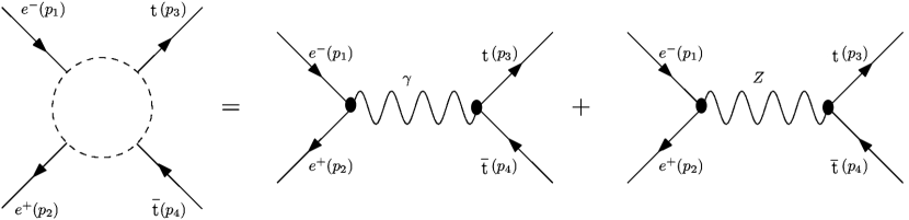
Figure 1: Feynman diagram for top quark pair production at linear colliders

The processes we consider are the tree-level processes and the external particles are on-shell. Applying the equation of motion to the external particles and using $\Theta_{\mu\nu}$ (given in equation 20), the Feynman rules are simplified as

$$i\,e\,Q_{e}\gamma_{\mu}\,\,$$ (25)

$$\frac{i\,e}{\sin 2\theta_{w}}\gamma_{\mu}(C_{ve}-C_{ae}\gamma_{5})$$ (26)

for $\gamma-e-e$ and $Z-e-e$ interaction vertices, respectively. Because of the specific choice of $\Theta_{\mu\nu}$ (equation 20), we find $p_{1}\Theta p_{2}=0$ and other momentum dependent simply vanishes by virtue of the equation of motion and the result turns out to be equivalent to the SM interaction. Here $Q_{e}$ is the electron charge and $C_{ve}$ and $C_{ae}$ are the vector and the axial-vector coupling of the electron with the $Z$ boson. On the other hand $p_{4}\Theta p_{3}\neq 0$, and we get

$$i\,e\,Q_{t}\gamma_{\mu}\,e^{i\frac{p_{4}\Theta p_{3}}{2}}-2\,\kappa\,e\,\gamma_{\mu}\sin\left(\frac{p_{4}\Theta p_{3}}{2}\right)$$ (27)

$$\frac{i\,e}{\sin 2\theta_{w}}\gamma_{\mu}(C_{vt}-C_{at}\gamma_{5})\,e^{i\frac{p_{4}\Theta p_{3}}{2}}+2\,\kappa\,e\,\tan\theta_{w}\,\gamma_{\mu}\sin\left(\frac{p_{4}\Theta p_{3}}{2}\right)$$ (28)

for $\gamma-t-t$ and $Z-t-t$ vertices respectively. Here $Q_{t}$ is the top quark charge and $C_{vt}$ and $C_{at}$ are the vector and the axial-vector couplings of the top quark with the $Z$ boson. Note that $C_{vf}=T_{3f}-2Q_{f}sin^{2}\theta_{w}$ and $C_{af}=T_{3f}$, where $f=e,t$.

Top pair differential cross section
The top pair production proceeds via the $s$ channel exchange of photon($\gamma$) and $Z$ boson and the tree level Feynman diagrams are shown in the Fig.1. The total noncommutative differential cross section can be written as

$$\frac{d\sigma^{NC}}{d\Omega}=\frac{d\sigma^{\gamma}}{d\Omega}+\frac{d\sigma^{Z}}{d\Omega}+\frac{d\sigma^{\gamma Z}}{d\Omega}.$$

The detailed calculations of NC differential cross section are given in the appendix A.2. The signature of the noncommutativity arises due to the term $\frac{p_{4}\Theta p_{3}}{2}=\left(\frac{s\,\beta}{4\Lambda^{2}}\right)\sin\theta\,\cos\phi$. Here $\theta$ is the polar angle which is defined with respect to the electron beam axis i.e along the $z$-axis and $\phi$ is the azimuthal angle. Since $\frac{d\sigma^{NC}}{d\Omega}$ is proportional to the momentum $\Theta$ weighted product $p_{4}\Theta p_{3}$, the azimuthal distribution possibly throw some light for probing the fermion non-minimal coupling $\kappa$ as a noncommutative signal.

3 Inferring the $\Theta$-exact NC coupling $\kappa$ and NC scale $\Lambda$

The $\Theta$-exact covariant non-minimal coupling $\kappa$ appears linearly in the differential cross section expressions from equations 52-57, while the NC scale ($\Lambda$) arises in the argument of the oscillatory function. In fact, there is no correlation between the non-minimal coupling $\kappa$ and the NC scale $\Lambda$. To see this, let us consider the photon mediated process,the differential cross section of which is given in equation 52. It has the term $4\,\kappa(\kappa+Q_{t})$. Notice that, the NC contribution will vanish either for $\kappa=0$ or $\kappa=-Q_{t}$ for all values of $\Lambda$. In the $V-A$ vertex, direct and interference terms of the differential cross-section, the coupling $\kappa$ appears as a linear function. To analyze the noncommutative effect, we next construct the NC correction observable

$$\Delta\sigma=\sigma^{NC}-\sigma^{SM}$$

In Fig.2, we have made the contour plot in the plane of $\kappa$ and $\Lambda$ corresponding to different $\Delta\sigma$ values which ranges from $10\%$ to $30\%$ correction with respect to

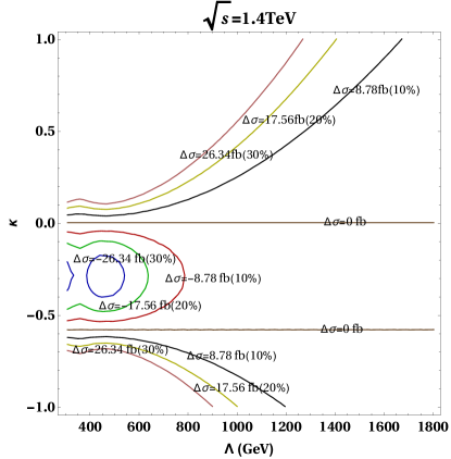
Figure 2: The figure depicts the correction in NC cross-section ($\Delta\sigma$ in fb) with respect to the standard model ($\sigma_{SM}^{1.4}=87.833\,fb,\,\sigma_{SM}^{3.0}=19.402\,fb$) in the presence of non-vanishing covariant $\theta$-exact coupling $\kappa$ at CLIC for $\sqrt{s}=1.4$ TeV (Left plot) and for $\sqrt{s}=3.0$ TeV (Right plot) respectively. Also shown the percentage of corresponding correction with respect to SM within the brackets.

SM cross section corresponding to the machine energy $\sqrt{s}=1.4$ TeV and $\sqrt{s}=3.0$ TeV, respectively. We see that the lower bound on $\Lambda$ increases with $\kappa$ as long as $\kappa$ is positive. From the plot, we find that the NC contribution vanishes at $\kappa=0$ and $\kappa\simeq-0.596$. This behaviour can be understood from the photon mediated process whose contribution is the predominant one. Here, specific domain of negative $\kappa$, exhibits the negative residual NC effects ($\Delta\sigma=-ve$), null effects i.e. $\Delta\sigma=0$ and positive residual NC effects ($\Delta\sigma=+ve$) as shown in Fig.2 for distinctive range of $\Lambda$ corresponding to the machine energy $\sqrt{s}=1.4$ TeV and $\sqrt{s}=3.0$ TeV, respectively. The negative residual cross section tells that the SM cross section is greater than the NC cross section. So we can classify the $\kappa$ parameter region as the region where the coupling ($\kappa$) is positive, the residual cross section is positive and the region where the coupling ($\kappa$) is negative, the residual cross section can be either negative, zero or positive. The negative residual effect, bounded by the region $\kappa\in[0,-0.596]$, gives rise a lower bound on the NC scale $\Lambda$. In the negative $\kappa$ region, as $\kappa$ increases from $0$ to $\kappa_{max}$, for a given $\Delta\sigma$, the lower bound on $\Lambda$ increases, and it then start decreases as $\kappa$ varies from $\kappa_{max}$ up to $-0.596$ it decreases the lower bound on $\Lambda$. For $\kappa_{max}=-0.298$, one finds the lower bound on NC scale as $\Lambda\geq 780(1680)$ GeV (at the machine energy $\sqrt{s}=1.4(3.0)$TeV) corresponding to $\Delta\sigma\sim 10\%$. On the other hand the positive residual effects are monotonically increasing (decreasing) effects in the region where $\kappa\geq 0$ ($\kappa\leq-0.596$).

3.1 Optimal collision energy

The positive residual region in the Fig.2 illustrates the monotonic behaviour of the coupling $\kappa$ with respect to the NC scale $\Lambda$, but it does not pinpoint where one can look for the NC signature. In contrast, it is not easier to locate the NC signature by arbitrarily scanning over the wide range of the collision energy. In Fig.3 (Left plot), the positive Kurtosis distribution exhibits that the NC contribution in the top pair production cross section first increases with the machine energy and then starts decreasing after a certain threshold machine energy for a specific value of $\Lambda$ at a fixed coupling $\kappa$.

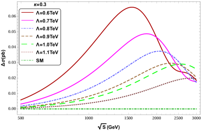
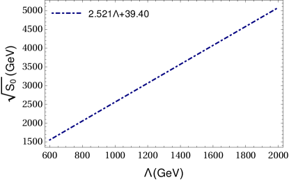
Figure 3: The left figure shows that the difference between NC total cross section and SM cross section ($\Delta\sigma=\sigma_{NCSM}-\sigma_{SM}$) as of a function of machine energy $\sqrt{s}$ and right figure shows probe of NC effects at optimum collision energy respectively.

It is true for all value of $\Lambda$ and $\kappa$. This machine threshold energy (also called the optimal machine energy) may be quite useful to look for the signature of the spacetime noncommutativity. One can obtain the linear relation by connecting all optimal collision energy (say $\sqrt{s_{0}}$) for respective value of the NC scale $\Lambda$ for a given $\kappa$. The optimal collision energy expressions for different $\kappa$ value can be written as

$$\sqrt{s_{0}} = 2.52151\,\Lambda+39.067\,\quad\,(\kappa=0.1)$$ (29)

$$\sqrt{s_{0}} = 2.52105\,\Lambda+39.443\,\quad\,(\kappa=0.3)$$ (30)

$$\sqrt{s_{0}} = 2.52107\,\Lambda+39.428\,\quad\,(\kappa=0.5)$$ (31)

Here the NC scale $\Lambda$ and the optimum collision energy $\sqrt{s_{0}}$ are in units of GeV. Notice that the optimal collision energy abruptly follows $2.5$ times (approx) the NC scale $\Lambda$. The Fig.3 (Right plot) shows that the allowed region (below line) of optimum lower limit of the NC scale which is obtained by optimum condition. These optimum region are not necessarily lower limit of the NC scale because the amount of NC cross section correction ($\bigtriangleup\sigma$) is not taken into account. Further, Fig.3 (Left plot) attains optimum point at certain value of machine energy ($\sqrt{s}$) for each NC scale which is known as optimum lower limit. This is the evident of the $TeV$ scale spacetime noncommutativity which is residing under the line $2.5\,\Lambda$ (approx). The positive value of $\kappa$ doesn’t affect the optimal collision energy relation but it plays an important role in the magnitude of the excess total cross section (see Fig.2). We see that one requires the collision energy to be greater than the NC scale in order to probe the spacetime noncommutativity at the future collider.

3.2 Inferring $\kappa$ in the light of azimuthal anisotropy

The azimuthal angular distribution of the top quarks pair (after reconstructing the $p_{T}$ of the top quark) can be an useful tool to probe the beyond the standard model (BSM) physics. Since $\Theta^{0i}\neq 0$ in our $\Theta^{\mu\nu}$ structure which is invariant under VSR Lorentz group symmetry, it makes NC theory rotationally non invariant.

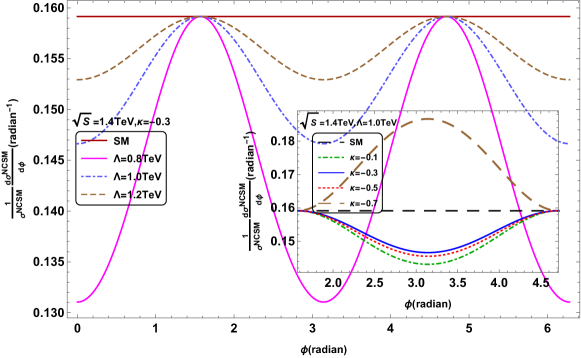
Figure 4: The figure shows normalized azimuthal anisotropy when $\kappa=-0.3$ at $\sqrt{s}=1.4$TeV. Inset shows that the normalized azimuthal anisotropy for $\kappa<0$ and the azimuthal angle $\phi$ taken between $\frac{\pi}{2}$ and $3\frac{\pi}{2}$.

Here the non zero $\Theta^{0i}$ produces the azimuthal anisotropy through momentum weighted $\Theta$ product which is $p_{4}\Theta p_{3}$. The amplitude of the anisotropy is gradually decreases by $f(1/\Lambda^{2})$. Depending up on the values of $\kappa$, the normalized azimuthal distribution has two different behaviour which is $\cos^{2}(f(1/\Lambda^{2})\cos[\phi])$ for $0>\kappa>-0.596$ in Fig.4 and $\sin^{2}(f(1/\Lambda^{2})\cos[\phi])$ for $\kappa>0$ and $\kappa<-0.596$ in Fig.5.

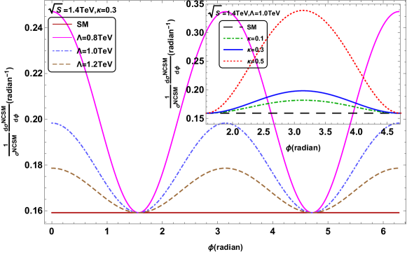
Figure 5: Same as Fig.4 for $\kappa=0.3$ at $\sqrt{s}=1.4$TeV. Inset shows that the normalized azimuthal anisotropy for $\kappa>0$ and the azimuthal angle $\phi$ taken between $\frac{\pi}{2}$ and $3\frac{\pi}{2}$.

This behaviour dominantly coming from equation 52 in the domain $0>\kappa>-0.596$ and $\kappa>0$ and $\kappa<-0.596$ respectively. However, the prediction of the signature of spacetime noncommutativity in these two domain are quite different. The domain $\kappa>0$ has discussed in the above Sec.3.1 and the allowed region of the optimum lower bound on $\Lambda$ are shown in Fig.3 (Right plot). The statistical analysis is the prominent way to find the signature of the spacetime noncommutativity which can be considered in the domain where $0>\kappa>-0.596$. So one can choose the azimuthal anisotropy as an observable to do statistical analysis namely $\chi^{2}$ analysis. The azimuthal asymmetry would give the fluctuated (excess or less) number of events around standard model flat value from $\phi=0$ to $\phi=2\pi$.

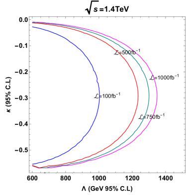
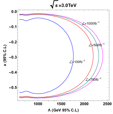
Figure 6: The left (right) figure depicts $\chi^{2}$ statistical test ($95\%C.L$) of the noncommutative signal event arises due to azimuthal anisotropy at $\sqrt{s}=1.4$ TeV ($\sqrt{s}=3.0$ TeV).

Here we have taken twelve bins, each has $\phi=\pi/6$ and totally eleven d.o.f in the $\chi^{2}$ value. The $\chi^{2}$ has defined as

$$\chi^{2}(\Lambda)=\sum_{i=1}^{12}\frac{(N_{i}^{NCSM}(\Lambda)-N_{i}^{SM})^{2}}{N_{i}^{SM}};\quad\,\quad N_{i}=\mathcal{L}\int\frac{d\sigma_{i}}{d\phi}d\phi$$

The Fig.6 depicts the statistical value of $\chi^{2}_{0.050}=19.675$ for both $\sqrt{s}=1.4$ TeV and $\sqrt{s}=3.0$ TeV for given integrated luminosity $\mathcal{L}$. Thus the luminosity contours excludes the lower bound at $95\%$ confidence level in the $\kappa-\Lambda$ plane.

Integrated luminosity ($\mathcal{L}$)	$100\,fb^{-1}$	$500\,fb^{-1}$	$750\,fb^{-1}$	$1000\,fb^{-1}$
Lower limit on $\Lambda$: $\sqrt{s}=1.4$TeV	$1.011\,TeV$	$1.235\,TeV$	$1.306\,TeV$	$1.352\,TeV$
Lower limit on $\Lambda$: $\sqrt{s}=3.0$TeV	$1.775\,TeV$	$2.20\,TeV$	$2.318\,TeV$	$2.406\,TeV$

Table 1: The lower bound on noncommutative scale $\Lambda$ ($95\%$C.L) obtained by $\chi^{2}$ analysis at $\kappa_{max}=-0.296$ for four different integrated luminosity.

The lower limit on the NC scale $\Lambda$ ($95\%$C.L) at $\kappa_{max}=-0.296$ is given below in table.1. Here one can notice that the noncommutative scale is sensitive to the integrated luminosity ($\mathcal{L}$) which is more clearly given in the Fig.13. The slope of the luminosity curve in the Fig.13 (red curve) is smaller in the higher luminosity region than the lower luminosity region. Such type of luminosity sensitivity has noticed in Zahra ; PTEP . In PTEP , authors considered profile likelihood ratio for two hypothesis test which is signal$+$background and background. We consider the background events as a SM $t\overline{t}$ pair events, thus our analysis simply boils down in to $\chi^{2}$. So one can compare the behaviour of $\Lambda$ from those two different approaches which are quite same results though they are different final production states too.

4 Helicity amplitude techniques in $\Theta$-exact NCSM

The study of polarization allows us to probe the chirality of the interactions between the top quark and gauge bosons in the SM as well as NCSM. The top polarization can be clearly analyzed in the $e^{-}e^{+}$ collider from $t\,\overline{t}$ pair production. We define the spin of the top quark and anti-top quark as shown in the Fig.7 at the production plane, so the transverse momentum of the top quark is zero and the spin four-vectors are back to back in the center of mass frame.

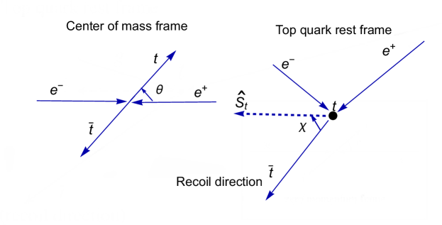
Figure 7: Top and anti-top production in the COM frame and top spin vector in the top rest frame.

Here $\widehat{s}$ is the spin vector of the top quark which makes an angle $\chi$ with anti-top quark in the recoil direction. In the special case, we take the spin angle $\chi=0$ or $\pi$, which tells that the spin direction is along the direction of the top quark momentum and it defines the helicity states of the top quark in the $t\,\overline{t}$ rest frame. If the massive top quark four momentum is $P^{\mu}=(E;\,\overrightarrow{\textbf{p}})$ then the spin four-vector defined asHaber ; HelicLC

$$s^{\mu}=(2\lambda)\frac{1}{m}(|\overrightarrow{\textbf{p}}|;\,E\,\widehat{\textbf{p}})$$ (32)

Here $(2\lambda)=\pm 1$ is the twice of the spin $1/2$ particle helicity ($\lambda$) and the spin four-vector satisfies $s.p=0$ and $s.s=-1$. One can derive the helicity projection operators as follows

$$u(p,\lambda)\,\overline{u}(p,\lambda) = \frac{1}{2}(1+\gamma_{5}\not{s})(\not{p}+m)$$ (33)

$$v(p,\lambda)\,\overline{v}(p,\lambda) = \frac{1}{2}(1+\gamma_{5}\not{s})(\not{p}-m)$$ (34)

Here we works in the commutative limit of the spacetime noncommutativity which does not change the Lorentz structure of the top quark spin. The generic differential cross section in the helicity amplitude technique at the center of mass frame (CM) for $a(\lambda_{a})+b(\lambda_{b})\longrightarrow c(\lambda_{c})+d(\lambda_{d})$ is

$$\frac{d\sigma}{d\Omega_{CM}}=\frac{1}{64\pi\,s}\left(\frac{p_{f}}{p_{i}}\right)\sum_{\lambda_{a}\lambda_{b}\lambda_{c}\lambda_{d}}|\mathcal{M}_{\lambda_{a}\lambda_{b};\lambda_{c}\lambda_{d}}|^{2}$$

Here $p_{i}(p_{f})$ is the initial (final) CM momentum, $\sqrt{s}$ is the CM-energy and $d\Omega_{CM}=d\cos\theta d\phi$. The detailed expressions for matrix element squared of all non vanishing helicity states are given in the appendix A.3.

4.1 Helicity correlation and top quark left-right asymmetry

Helicity correlation
The top quark is the heavier quark in the standard model. It decays weakly into $b$ quark and $W$ boson before hadranization process happens. In fact the lifetime ($\tau_{t}\approx 5\times 10^{-25}$s) of the top quark is lesser than hadranization time ($\tau_{QCD}\approx 1/\Lambda_{QCD}=(200\,MeV)^{-1}\approx 3.3\times 10^{-24}$s)Peskin ; Bigi ; spincorr as well as spin-decorrelation time ($\tau_{spin}\approx m_{t}/\Lambda^{2}_{QCD}\approx 3\times 10^{-21}$s) from spin-spin interactions with the light quarks generated in the fragmentation processspincorrbook ; D0 .

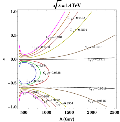
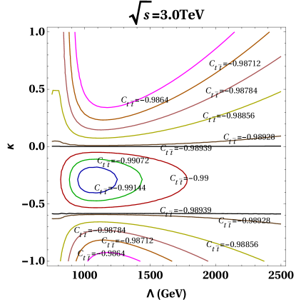
Figure 8: Helicity correlation between the top and anti-top quark.

If the top quark spins are correlated when they are produced as a pair then their decay products are correlated with their spin and hence the decay products of the top quarks are correlated by naturally. The $t\,\overline{t}$ spin correlation reported in the CDF II detector CDFII ; D0 by reconstructing lepton plus jets decay channel from $p\,\overline{p}$ collisions. The measurement agrees with the SM QCD calculation by adding gluon fusion process. But the decay width of the top quark has deviation from SM calculationCDF . In the case of spacetime noncommutativity, the top decay were studied in the minimal $\Theta$-expanded NCSMnamit ; najafa ; Zahra2 .
However this non-minimal $\Theta$-exact SW map approach will not participate in the tree level top decay, it appears only in the loop level. Since there is no right-handed $W$ boson in the NCSM and we extended non-minimal star product among abelian gauge field and SM fermions with satisfying the gauge transformation which is given in equation.13, one cannot have a non-minimal coupling $\kappa$ with top quark in the charged current. Thus the effect of spacetime noncommutativity on spin correlation can be determined from the top quark pair production.

Considering the top pair production, the measured spin correlation depends on the choice of the spin basis. There are three types of basisParkelc , which are i) beam line basis ii) helicity basis and iii) off-diagonal basis. Here we work in the helicity basis (which admits the center of mass frame in which the top spin axis is defined) to find the top quark spin correlation. The helicity correlation factor defined asParkelc ; Parkelhc

$$C_{t\overline{t}}=\frac{\sigma_{LL}+\sigma_{RR}-\sigma_{LR}-\sigma_{RL}}{\sigma_{LL}+\sigma_{RR}+\sigma_{LR}+\sigma_{RL}}$$ (35)

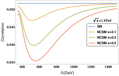
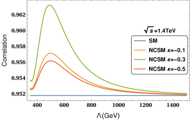
Figure 9: Helicity correlation ($|C_{t\overline{t}}|$) between the top and anti-top quark at $\sqrt{s}=1.4$ TeV in the presence of positive values of non-minimal coupling $\kappa$ (Left plot) and also negative (Right plot).

Here $\sigma_{ij}\quad(i,j=L,R)$ represents the total cross section of the final state top, anti-top helicity. Notice that $\sigma_{LL}\equiv\sigma_{RR}=0$ when $\beta=1$ i.e $\sqrt{s}>>m_{t}$ which is ultra-relativistic limit. In the ultra-relativistic limit, the helicity correlation is $C_{t\overline{t}}=-1$ when $LR$ configuration equals to $RL$ configuration in the $t\overline{t}$ pair production which are solely due to left-right helicity symmetry at high energy.

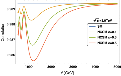
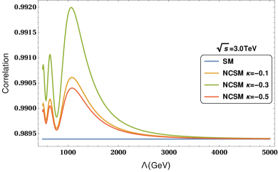
Figure 10: Same as Fig.9 for $\sqrt{s}=3.0$ TeV.

The top quark SM helicity correlation as shown in Fig.8, which are $C_{t\overline{t}}=-0.9518(-0.9894)$ at $\sqrt{s}=1.4(3.0)$ TeV respectively. Here the negative sign emphasize that the opposite final state helicity cross section are usually dominant over the one with same helicity final state cross section in the $e^{-}e^{+}$ colliders. In the region where $\kappa>0$ and $\kappa<-0.596$, the NC helicity correlation is lesser than the SM helicity correlation for all values of NC scale $\Lambda$ and when $\Lambda\rightarrow\infty$ one recovers the SM results. The another region $0>\kappa>-0.596$, the value of $C_{t\overline{t}}$ reduces gradually when the NC scale increases. But here the NC helicity correlation are greater than the SM correlation.

Notice that the region $\Lambda<350$GeV at$\sqrt{s}=1.4$TeV and $\Lambda<800$GeV at$\sqrt{s}=3.0$TeV are excluded because which are arises due to unphysical oscillatory behaviour near lower values of NC scale. The top quark correlations for $\kappa>0$ and $\kappa<-0.596$ are given in Fig.9 and Fig.10 which shows that the optimal correlation values than SM value are located at $\Lambda\approx 520$ GeV ($\sqrt{s}=1.4$ TeV) and $\Lambda\approx 1150$ GeV ($\sqrt{s}=3.0$ TeV) respectively. Thus one can conclude that if any measured helicity correlation deviates from SM, our result will put a lower bound on NC scale which are $\Lambda\geq 520$GeV ($\sqrt{s}=1.4$TeV) and $\Lambda\geq 1150$GeV ($\sqrt{s}=3.0$TeV) respectively. The non-minimal coupling $\kappa$ can be arbitrary in the positive region which can be restricted by statistical significance of the experimental results but in the negative region it can be taken as $\kappa_{max}=-0.296$.

Top quark left-right asymmetry
In the top quark pair production, we can predict the dominant helicity of the top quark by calculating the top quark left-right asymmetry. The polarized top quark decay produced $b$ quark and longitudinally polarized $W$ boson dominantly. The ratio of the decay rate for polarized top quark and unpolarized top quark ($F_{0}=\left[\Gamma(t\rightarrow b\,W_{L})/\Gamma^{total}(t\rightarrow b\,W)\right]$) was measured by CDFCDF which is $F_{0}=0.91\pm 0.37\pm 0.13$. The SM value is $F_{0}=0.701$.

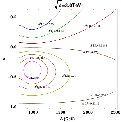
Figure 11: Final state top quark left-right asymmetry

In the non-minimal model, there is no change in the decay rate, however, it gives an insight about non-minimal coupling $\kappa$ and NC scale $\Lambda$ when left handed top quark produced from $e^{-}e^{+}$ annihilation. Thus it is useful to compute top quark left-right asymmetrytoplrasy1 ; toplrasy2 .

$$A^{t}_{LR}=\frac{\sigma(e^{-}e^{+}\longrightarrow t_{L}\overline{t})-\sigma(e^{-}e^{+}\longrightarrow t_{R}\overline{t})}{\sigma(e^{-}e^{+}\longrightarrow t\overline{t})}$$ (36)

In the numerator while obtaining cross section, we have summed over the initial state helicity for electron and positron as well as final state hecility of the anti-top quark except final state top quark helicity, in the denominator, we have summed over all the helicity states on the incoming and outgoing particles. In Fig.11, we have shown the contour plots in the $\kappa-\Lambda$ plane corresponding to different values of left-right asymmetry ($A^{t}_{LR}$) of top quark. The standard model $A^{t}_{LR}$ increases with the increase in the machine energy, as the production cross-section for left handed top quark is higher than the right handed top quark production at high energy limit. In the SM, one finds the top quark left-right asymmetry $20.8\%(21.45\%)$ at the machine energy $\sqrt{s}=1.4(3.0)$ TeV. In the negative $\kappa$ region, $\kappa_{max}\simeq-0.43$ we get the asymmetry $25\%$ (approx) corresponding to $\Lambda=840$ GeV at the machine energy $\sqrt{s}=1.4$ TeV. Similarly, for $\sqrt{s}=3.0$ TeV, one find asymmetry upto $28\%$ (approx) for $\Lambda=1670$ GeV.

4.2 Polarized beam analysis

In general, the electron and positron beams can have two types of polarizations which are transverse and longitudinal polarization. Since we consider the bunch of massless electrons as a beam at linear colliders, the transverse polarizations are negligible, thus one can define the total cross section with arbitrary longitudinal polarization ($P_{e^{-}},P_{e^{+}}$) given by

$$\sigma_{P_{e^{-}}P_{e^{+}}}=\frac{(1-P_{e^{-}})}{2}\frac{(1+P_{e^{+}})}{2}\sigma_{LR}+\frac{(1+P_{e^{-}})}{2}\frac{(1-P_{e^{+}})}{2}\sigma_{RL}$$ (37)

Where $\sigma_{LR}$ is the total cross section of the top pair production when the initial left-handed $e^{-}$ beams and initial right-handed $e^{+}$ beams are considered if fully polarized at $P_{e^{-}}=-1,P_{e^{+}}=+1$. The $\sigma_{RL}$ is defined analogously.

$$\sigma_{LR}=\sum_{h_{t},h_{\overline{t}}}\sigma_{L\,R\,h_{t}\,h_{\overline{t}}}\,\quad\,\sigma_{RL}=\sum_{h_{t},h_{\overline{t}}}\sigma_{R\,L\,h_{t}\,h_{\overline{t}}}$$ (38)

Here $h_{t}$ and $h_{\overline{t}}$ correspond to the helicity states of the top and anti-top quarks, which are summed over.The total cross section will enhance when electron and positron beams are polarized and the signs of $P_{e^{-}}$ and $P_{e^{+}}$ are opposite. This can be realized when the total cross section written in terms of effective polarization as given belowHaber ; HelicLC .

$$\sigma_{P_{e^{-}}P_{e^{+}}}=(1-P_{e^{-}}P_{e^{+}})\sigma_{0}(1-P_{eff}A_{LR})$$

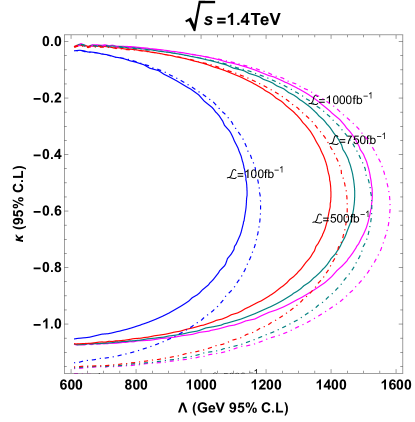
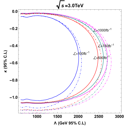
Figure 12: The figure depicts $\chi^{2}$ statistical test ($95\%C.L$) of polarized the noncommutative signal event arises due to azimuthal anisotropy only considering the $-^{ve}$ region of the $\kappa$.The color line corresponds to $P_{e^{-}}=-80\%,P_{e^{+}}=30\%$ and dot-dashed color line corresponds to $P_{e^{-}}=-80\%,P_{e^{+}}=60\%$ for various integrated luminosity $\int\mathcal{L}\,dt=100({\color[rgb]{0,0,1}blue}),\,500({\color[rgb]{1,0,0}red}),\,750({\color[rgb]{0,0.5,0.5}cyan})\,fb^{-1}$ and $1000({\color[rgb]{1,0,1}megenta})\,fb^{-1}$ at CLIC $\sqrt{s}=1.4$ TeV (left) and $\sqrt{s}=3.0$ TeV (right).

Integrated luminosity ($\mathcal{L}$)	$100\,fb^{-1}$	$500\,fb^{-1}$	$750\,fb^{-1}$	$1000\,fb^{-1}$
$\kappa_{max}=-0.5445$ and $P_{\{e^{-},e^{+}\}}=\{-0.8\,,\,0.3\}$
Lower limit on $\Lambda$: $\sqrt{s}=1.4$TeV	$1.131\,TeV$	$1.390\,TeV$	$1.462\,TeV$	$1.517\,TeV$
Lower limit on $\Lambda$: $\sqrt{s}=3.0$TeV	$2.000\,TeV$	$2.474\,TeV$	$2.606\,TeV$	$2.703\,TeV$
$\kappa_{max}=-0.607$ and $P_{\{e^{-},e^{+}\}}=\{-0.8\,,\,0.6\}$
Lower limit on $\Lambda$: $\sqrt{s}=1.4$TeV	$1.172\,TeV$	$1.440\,TeV$	$1.514\,TeV$	$1.570\,TeV$
Lower limit on $\Lambda$: $\sqrt{s}=3.0$TeV	$2.075\,TeV$	$2.560\,TeV$	$2.70\,TeV$	$2.80\,TeV$

Table 2: The lower bound on noncommutative scale $\Lambda$ ($95\%$C.L) and $\kappa_{max}=\{-0.5445\,,\,-0.607\}$ obtained by $\chi^{2}$ analysis when $P_{\{e^{-},e^{+}\}}=\{-0.8\,,\,0.3\}$ and $P_{\{e^{-},e^{+}\}}=\{-0.8\,,\,0.6\}$ for four different integrated luminosity.

Here the unpolarized total cross section $\sigma_{0}=(\sigma_{LR}+\sigma_{RL})/4$, left-right asymmetry $A_{LR}=(\sigma_{LR}-\sigma_{RL})/(\sigma_{LR}+\sigma_{RL})$ and effective polarization $P_{eff}=(P_{e^{-}}-P_{e^{+}})/(1-P_{e^{-}}P_{e^{+}})$. The $P_{eff}$ can be achieved $-1$ when $P_{e^{-}}=-1.0\,,P_{e^{+}}=0.0$ and $P_{e^{-}}=-1.0\,,P_{e^{+}}=1.0$. So that the total cross section enhanced by $\sigma_{\{-1,0\}}=\sigma_{0}+\sigma_{0}\,A_{LR}$ and $\sigma_{\{-1,1\}}=2(\sigma_{0}+\sigma_{0}\,A_{LR})=2\sigma_{\{-1,0\}}$ respectively. In the future linear colliders, the polarization can be studied with $P_{e^{-}}=-0.8\,,P_{e^{+}}=0.3$ and $P_{e^{-}}=-0.8\,,P_{e^{+}}=0.6$ which will enhance the total cross section significantly by following expressions

$$\sigma_{\{-0.8,0.3\}} = 1.24\,\sigma_{0}+1.1\,\sigma_{0}\,A_{LR}$$ (39)

$$\sigma_{\{-0.8,0.6\}} = 1.48\,\sigma_{0}+1.4\,\sigma_{0}\,A_{LR}$$ (40)

Note that the above set of equations are same for all new physics as well as for the standard model. The beam polarization enhances the new physics signal ($S$) and suppresses the background ($B$) rates by significant increment of $S/B$ or $S/\sqrt{B}$.

In our analysis $\sigma_{0}$ and $A_{LR}$ are function of $\Lambda$. We made $\chi^{2}$ test for polarized beam analysis by keeping the azimuthal anisotropy as an observable. The polarization enhances the lower limit on NC scale and non minimal coupling $\kappa_{max}$ also. The lower bound on noncommutative scale is given in the table.2 for four values of integrated luminosity.

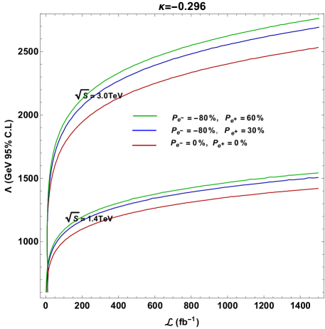
Figure 13: The figure depicts $\chi^{2}$ statistical test ($95\%C.L$) of polarized noncommutative signal event arises due to azimuthal anisotropy.

The sensitivity of the NC scale $\Lambda$ on integrated luminosity of the polarized electron positron beam has given in the Fig.13. In the above Fig.12 we have seen that the polarization has pushed $\kappa_{max}=-0.296$ into $\kappa_{max}=-0.607$ when $P_{\{e^{-}\,,\,e^{+}\}}=\{-0.8\,,\,0.6\}$. But one can compare the lower bound on NC scale with the unpolarized beam and partially polarized beam luminosity for fixed value of $\kappa_{max}$ at $-0.296$ which is shown in the Fig.13. There are significant enhancement in the lower limit of the NC scale. If any one of the beam fully polarized and another one has unpolarized (fully polarized) which gives $P_{eff}=100\%$ and one can get two (four) times enhancement in the total cross section.

5 Summary and conclusion

We study the top quark pair production $e^{+}e^{-}\stackrel{{\scriptstyle\gamma,Z}}{{\longrightarrow}}t\overline{t}$ at the TeV energy linear collider in the non-minimal NCSM within the framework of covariant $\Theta$-exact Seiberg-Witten approach. Although the NC tensor $\Theta_{\mu\nu}$ breaks the rotational invariance due to $\Theta_{0i}\neq 0$, however, it preserves the translational symmetry which is invariant under the $T(2)$ subgroup of VSR. We study the NC cross section correction observable $\Delta\sigma=\sigma^{NC}-\sigma^{SM}$ corresponding to the machine energy $\sqrt{s}=1.4$ TeV as well as $\sqrt{s}=3.0$ TeV, and presented our result in terms of the non-minimal coupling $\kappa$ and the NC scale $\Lambda$ corresponding to positive and negative $\Delta\sigma$. For $\kappa_{max}=-0.296$, we find the lower bound on the NC scale $\Lambda\geq 780(1680)$ GeV corresponding to $\Delta\sigma\sim 10\%$ at the machine energy $\sqrt{s}=1.4(3.0)$ TeV. For a specific value of $\Lambda$ at a fixed positive coupling $\kappa$, we found a specific optimal collision energy relation which is $\sqrt{s_{0}}=2.52105~{}\Lambda+39.443$, may be quite useful to look for the signature of the spacetime noncommutativity. The normalized azimuthal distribution is found to vary according to $cos^{2}[f(1/\Lambda^{2})sin\theta cos\phi]$ for $0>\kappa>-0.596$ and $sin^{2}[f(1/\Lambda^{2})sin\theta cos\phi]$ for $\kappa>0$ and $\kappa<-0.596$. A statistical $\chi^{2}$ analysis of the azimuthal anisotropy gives rise a lower bound on $\Lambda=1.0,~{}1.2,~{}1.3,~{}1.35$ TeV corresponding to linear collider luminosity ${\mathcal{L}}=100,~{}500,~{}750,~{}1000~{}\rm{fb^{-1}}$ for $\kappa_{max}=-0.296$ at the machine energy $\sqrt{s}=1.4$ TeV.
We perform a detailed helicity analysis of the $t~{}\overline{t}$ production. We present the helicity correlation $C_{t{\overline{t}}}$ of the final state top quark and anti-top quark produced with a certain helicity and found that such a correlation which is constant at $\sqrt{s}=1.4(3.0)$ TeV i.e. $C^{SM}_{t{\overline{t}}}=-0.9518\,,\,(-0.9894)$ respectively, varies with the NC scale $\Lambda$ for different coupling constant $\kappa$ in the NCSM.We investigate the sensitivities of the top quark left-right asymmetry $A^{t}_{LR}$ on the non-minimal coupling $\kappa$ and the NC scale $\Lambda$ and find that the asymmetry is about $25\%$ in the non-minimal NCSM with $\kappa_{max}=-0.43$ corresponding to $\Lambda=840~{}$ GeV at the machine energy $\sqrt{s}=1.4$ TeV. Further, we perform a detailed $\chi^{2}$ analysis for the polarized electron-polarized beam with $P_{e^{-}}=-80\%$ and $P_{e^{+}}=60\%$ corresponding to the machine energy $\sqrt{s}=1.4~{}(3.0)$ TeV for different machine luminosities. We obtain the lower bound on $\Lambda=1.17(2.08),~{}1.44(2.56),~{}1.51(2.70),~{}1.57(2.80)$ corresponding to the machine luminosity ${\mathcal{L}}=100,~{}500,~{}750,~{}1000~{}\rm{fb^{-1}}$ for $\kappa_{max}=-0.607$. Finally, we studied the intriguing mixing of the UV and the IR by invoking a specific structure of noncommutative anti-symmetric tensor $\Theta_{\mu\nu}$ which is invariant under translational $T(2)$ VSR Lorentz sub group given in the appendix A.1.

Appendix A Removal of UV/IR mixing and NC helicity amplitude calculation

A.1 Removal of UV/IR mixing in the one loop calculation

There are several attempts has been made to solve/remove the UV/IR mixing which are appears as phase factor due to Moyal product between NC fields in the spacetime noncommutative field theory. In the $\Theta-$expanded Seiberg-Witten map approach, the UV/IR mixing disappears MWURIR1 ; SWURIR5 and the renormalibility has under control up to one loop $\mathcal{O}(\Theta)$. But in the case of $\Theta-$exact Seiberg-Witten map approach, the UV/IR mixing are present until the noncommutative tensor $\Theta^{\mu\nu}$ takes the special structure. The specific structure of the $\Theta^{\mu\nu}$ removes the both singularity in the $\Theta-$exact as well as covariant $\Theta-$exact noncommutative field theory which is given in SWURIR8 ; HKT3 ; SWURIR9 . But those structure of $\Theta^{\mu\nu}$ given in SWURIR8 ; SWURIR9 violates the VSR $T(2)$ translation property.

Here, we have shown that our choice of $\Theta^{\mu\nu}$ removes the UV/IR mixing which satisfy the translational invariant under VSR group. Since $\Theta^{0i}\neq 0$ in our case, thus the azimuthal anisotropy play an unique feature to probe the spacetime noncommutativity at particle colliders.
In order to remove the UV/IR mixing at one-loop self energy correction, R. Horvat et.al.,SWURIR9 ; HKT3 introduced non-minimal fermion coupling ($\kappa$) in the $U(1)$ gauge theory following manner

$$S^{U(1)}_{f}=\int-\frac{1}{4}f_{\mu\nu}f^{\mu\nu}+i\overline{\psi}\not{\partial}\psi-i\Theta^{ij}\overline{\psi}\gamma^{\mu}\left(\frac{1}{2}f_{ij}\circledast\partial_{\mu}\psi-\kappa f_{\mu i}\circledast\partial_{j}\psi\right)$$ (41)

Where $f_{\mu\nu}=\partial_{\mu}a_{\nu}-\partial_{\nu}a_{\mu}$. Eventually, we get following feyman rule for massless neutral fermion-fermion- photon interaction

$$-e\widetilde{F}_{\circledast}(p,q)\left[\kappa\left(\not{q}(\Theta p)^{\mu}-(q\Theta p)\gamma^{\mu}\right)-(\Theta q)^{\mu}\not{p}\right]$$ (42)

Here $p$ is the fermion momentum which flows towards vertex and $q$ is the photon incoming momentum. Note that

$$[f,g]_{\star}=i\Theta^{ij}\partial_{i}f\circledast\partial_{j}g$$

In principle,

$$[A_{\mu},\psi]_{\star}=A_{\mu}\star\psi-\psi\star A_{\mu}$$

Thus the covariant derivative for neutral fermion can be written as

$$D_{\mu}\psi=\partial_{\mu}\psi-i\kappa\,[A_{\mu},\psi]_{\star}$$

When $\kappa=0$, we get the commutative interaction which is not consider in eqn. 42. We can realize that $\kappa$ is the non-minimal NC coupling, the strength of the neutral fermion and abelian gauge field interaction is proportional to $\kappa\,e$, which is shown in eqn.23. We follow the $SU_{\star}(2)_{L}\otimes U_{\star}(1)_{Y}$ fermion action which is given in HKT1 ; HKT3 , allows the interaction between neutral right handed fermion and abelian gauge field in the constant anti-symmetric background field.

Figure 14: Neutral fermion (Neutrino) one-loop self energy Feynman diagram ($\Sigma_{1}$).

Let us consider the massless neutral fermion one-loop self energy correction in the covariant $\Theta-$exact NCSM as follows

$$\Sigma_{1} = -(\kappa\,e)^{2}\mu^{4-D}\int\frac{d^{D}q}{(2\pi)^{D}}\,\frac{-i\eta_{\mu\nu}}{q^{2}}\,\widetilde{F}_{\circledast}(p,q)\,\left[(q\Theta p)\gamma^{\mu}+\not{p}(\Theta q)^{\mu}-\not{q}(\Theta p)^{\mu}\right]\,\frac{i\not{p}+\not{q}}{(p+q)^{2}}$$ (43)

$$\widetilde{F}_{\circledast}(p,q)\left[-(q\Theta p)\gamma^{\nu}-\not{p}(\Theta q)^{\nu}+\not{q}(\Theta p)^{\nu}\right]$$

Where $\widetilde{F}_{\circledast}(p,q)=2\left(\frac{\sin((q\Theta p)/2)}{q\Theta p}\right)$. Our results and ref HKT3 results are differs only by multiplication factor which is $\kappa^{2}$. Apart from bubble diagram other tadpole one-loop diagrams ($\Sigma_{3}\,,\,\Sigma_{4}$) vanishes due to charge conjugation symmetry ($\Theta^{\mu\nu}_{C}=-\Theta^{\mu\nu}$) as shown in ref HKT3 . The four field tadpole (2-fermion 2-photon) one-loop ($\Sigma_{2}$) vanishes which can be easily viewed when $\eta_{\mu\nu}V^{\mu\nu}_{3}(p,-p,q,q)=0$, the four field interaction $V^{\mu\nu}_{3}(p,-p,q,q)$ can get from eqn (2.10) in refHKT3 . Eventually, the non-vanishing bubble diagram (as shown in fig.14) has to be evaluate. We follow

• presence of $q\Theta p$ dimensionless scalar quantity in the denominator, we use HQET parametrization HQET to combine all quadratic and linear denominator.

• we use Schwinger technique to turn the denominator into Gaussian integrals and absorb NC phase factor into that.

• we calculate all the integrals which are presented in the numerator by using Gradshteyn .

In field theory, if the Hamiltonian has positivity properties then we can analytically continue to imaginary values of time along adopting the Weyl’s unitarity trick which leads Euclidean field theory of causal propagation with positive energies. The analytic continuation is defined by the rotation of the vector in the complex plane an angle of $\pi/2$ about the origin namely Wick rotation. Therefore one can go from Minkowski spacetime to Euclidean spacetime by replacing the time $t$ by $i\,t$ and the energy $p^{0}$ by $i\,p^{0}$. In our NCQFT, the analytic continuation demands that the noncommutative space-time (NCST) component $\Theta^{0i}$ undergo $\Theta^{0i}\rightarrow-i\Theta^{0i}$ and leaves invariant Moyal phase ($q\Theta p$) under Wick rotation JT1 ; JT2 . Here the time component of four momenta undergo $q^{0}\rightarrow iq^{0}$ and $p^{0}\rightarrow ip^{0}$ by Wick rotation, $q$ is loop momenta and $p$ is external momenta. The noncommutative space-space (NCSS) component remains same like three-momenta ($p^{i}$) by Wick rotation. After Schwinger parametrization, we get the same Euclidean integrals which is shown in ref HKT3 . The integrals $I_{123}$ equation (A.1), $I_{456}$ equation (A.7) and $I_{789}$ equation (A.8) in ref HKT3 has to satisfy the important unitarity condition thereby the Euclidean term $(\widetilde{p})^{2}(=(\Theta p)^{2})$ should be positive. Such term arises from the Schwinger parametrization and redefined loop momenta $l$. The loop momenta $l$ is still invariant by Wick rotation using the dual property of VSR NC tensor i.e duality of NCST ($\Theta^{0i}$) and NCSS ($\Theta^{3i}$). We can back to Euclidean to Minkowski by analytic continuation. In order to do that, we have to prove $(\widetilde{p})^{2}$ is positive in Minkowski spacetime, otherwise the integral would not converge and can’t achieve unitarity JT1 ; JT2 . Our case we get,

$$\widetilde{p}^{2}=\frac{1}{\Lambda^{4}}(a^{2}+b^{2}).(p_{0}-p_{3})^{2}=\theta^{2}p_{-}^{2}\,\,\Longrightarrow\,\,\text{Always positive}$$

Here $a$ and $b$ are real and $\theta^{2}=\frac{1}{\Lambda^{4}}(a^{2}+b^{2})$ and $p_{-}$ is the back-ward lightcone momentum of the propagating neutral particle. Since $\widetilde{p}^{2}$ is positive, the Light like spacetime VSR noncommutativity obeys the unitarity property perturbatively. After long calculation we get simplified equation 43 for $D=4-\epsilon$ and in $\epsilon\rightarrow 0$ limit,

$$\Sigma_{1}=-(\kappa\,e)^{2}\gamma_{\mu}\left[p^{\mu}\mathcal{A}+(\Theta\Theta p)^{\mu}\frac{p^{2}}{(\Theta p)^{2}}\mathcal{B}\right]$$ (44)

Here

$$\mathcal{A} = \frac{1}{(4\pi)^{2}}\left[(S_{1}+2S_{2})\mathcal{A}_{1}+(1+S_{1}+S_{2})\mathcal{A}_{2}\right]$$ (45)

$$\mathcal{B} = -\frac{2}{(4\pi)^{2}}\mathcal{A}_{2}$$ (46)

$$\mathcal{A}_{1} = \frac{2}{\epsilon}+\ln\left(\pi e^{\gamma_{E}}\mu^{2}(\Theta p)^{2}\right)+\frac{1}{2}\sum_{k=1}^{\infty}\frac{\sqrt{\pi}}{\Gamma\left(k+1\right)\Gamma\left(k+\frac{3}{2}\right)}\left(\frac{p^{2}(\Theta p)^{2}}{16}\right)^{k}\mathcal{A}_{3}$$

$$\mathcal{A}_{2} = 2-\frac{1}{2}\sum_{k=0}^{\infty}\frac{\sqrt{\pi}\,\Gamma\left(k+\frac{1}{2}\right)}{\Gamma\left(k+1\right)\Gamma\left(k+\frac{3}{2}\right)\Gamma\left(k+\frac{5}{2}\right)}\left(\frac{p^{2}(\Theta p)^{2}}{16}\right)^{k+1}\left(\mathcal{A}_{3}+\psi_{0}\left(k+\frac{1}{2}\right)-\psi_{0}\left(k+\frac{5}{2}\right)\right)$$

$$\mathcal{A}_{3} = \ln\left(\frac{p^{2}(\Theta p)^{2}}{16}\right)-\psi_{0}\left(k+1\right)-\psi_{0}\left(k+\frac{3}{2}\right)$$ (47)

Where $\psi_{0}(z)$ are di-gamma functions and $\gamma_{E}\simeq-0.577215$ is Euler-Mascheroni constant. Further $S_{1}$ and $S_{2}$ are scale independent $\Theta$ ratios. We get the scalar quantity $\Theta_{\mu\nu}\Theta^{\mu\nu}$ in $S_{1}$ which arises after integrating the loop momenta.

$$S_{1}=p^{2}\frac{\Theta_{\mu\nu}\Theta^{\mu\nu}}{(\Theta p)^{2}}\,;\quad\,S_{2}=p^{2}\frac{(\Theta\Theta p)^{2}}{(\Theta p)^{4}};$$ (48)

We know that $(\Theta p)^{2}$ is always positive, then the above equations are valid in the Minkowski spacetime, Which means that the Euclidean 4D space results are same in the Minkowski 4D spacetime by analytic continuation according to Weyl’s trick in field theoryJT1 ; JT2 . By looking at the equation 17, one can conclude that $S_{1}=0$ and by using equation 20, we get $(\Theta\Theta p)^{2}=0$ for all value of $p$. The UV/IR mixing and hard $1/\epsilon$ UV divergence vanishes but IR divergence still present in the NC theory.

$$\Sigma_{1}=(\kappa\,e)^{2}\frac{1}{(4\pi)^{2}}\left[\not{p}-2\not{\tipaupperaccent[-.2ex]{3}{\tipaupperaccent{3}{p}}}\frac{p^{2}}{(\Theta p)^{2}}\right]\mathcal{A}_{2}$$ (49)

Here $\tipaupperaccent[-.2ex]{3}{\tipaupperaccent{3}{p}}^{\mu}=(\Theta\Theta p)^{\mu}=\Theta^{\mu\nu}\Theta_{\nu\rho}p^{\rho}$. Interestingly, $\not{\tipaupperaccent[-.2ex]{3}{\tipaupperaccent{3}{p}}}$ can be written as $\frac{(\tipaupperaccent[-.2ex]{3}{\tipaupperaccent{3}{p}})^{2}}{\not{\tipaupperaccent[-.2ex]{3}{\tipaupperaccent{3}{p}}}}$, and $(\tipaupperaccent[-.2ex]{3}{\tipaupperaccent{3}{p}})^{2}=0\,\forall\,p$ by VSR, thereby the quadratic IR singularity disappears. At last, we have arrived the logarithmic IR singularity with convergent sum of $f^{k}(p,\widetilde{p})$ as follows,

$$\Sigma_{1}=(\kappa\,e)^{2}\frac{\not{p}}{8\pi^{2}}\left[1-\frac{\sqrt{\pi}}{4}\,\left(\frac{p^{2}\widetilde{p}^{2}}{16}\right)\left\{\ln\left(\frac{p^{2}\widetilde{p}^{2}}{16}\right)\sum_{k=0}^{\infty}\,f^{k}(p,\widetilde{p})+\sum_{k=0}^{\infty}\,\psi_{0}^{k}\,f^{k}(p,\widetilde{p})\right\}\right]$$ (50)

$$\text{Here}\,f^{k}(p,\widetilde{p})=\frac{\left(\frac{p^{2}\widetilde{p}^{2}}{16}\right)^{k}\,\Gamma\left(k+\frac{1}{2}\right)}{\Gamma\left(k+1\right)\Gamma\left(k+\frac{3}{2}\right)\Gamma\left(k+\frac{5}{2}\right)}\,,\,\,\text{ and}\,\,\psi_{0}^{k}\,\,\text{is related to di-gamma function, }$$

$$\text{which is }\,\,\psi_{0}^{k}=\psi_{0}(k+1/2)-\psi_{0}(k+1)-\psi_{0}(k+3/2)-\psi_{0}(k+5/2)$$

The IR divergence pay the attention on motion of the particle inside noncommutative plane which results that the spatial extension $\Theta p$ cannot shrink to zero SWURIR8 . On the other hand, the IR singularity can be removed by re-summing the propagator analogous to finite temperature field theory and introducing appropriate counter term in the interaction Lagrangian. We will discuss more in the near future work.

In the scalar field theory, the mass of the scalar is far from UV scale, thus one can think of the naturalness of the scalar mass UV physics knows nothing about the theory in the far IR. Instead of introducing the new symmetries and extra-dimensions one might hope that connecting the far IR and far UV can solve the naturalness problem craig . Interestingly, the NCQFT and quantum gravity exhibit the UV/IR mixing by its nature. Recently proposed weak gravity conjecture (WGC) vafa ; WGC on the form of hierarchical UV/IR mixing restricts the mass of the scalar to a IR scale far below the UV scale which is associated to quantum gravity. Here we have given a glimpse of WGC on non-vanishing NC scale parameter $\Theta$ which was considered in qhuang ; mli . Consider the construction of the soliton in $2+1$ dimensional NC scalar field theory, in general $2l+1$ dimensional theorysoliton1 ; soliton2 one can understand the feature of the NC parameter $\Theta$. Where $l$ is $1,2,...$ According to Derrick theorem, the kinetic and potential energies are decreases when all length scale are shrinks as $L\rightarrow\lambda L$, consequently no finite-size minimum can occur at $\lambda\rightarrow 0$. But in the NC scenario, the Derrick theorem fails by existence of classically stable GMS soliton soliton1 ; soliton2 in the presence of distinguished length scale $\sqrt{\Theta}$ especially in $2+1$ spacetime. Here $\Theta$ is the eigen value of the $\Theta^{\mu\,\nu}$. In the weak gravity limit, the soliton is presented in the two-dimensional consistent quantum gravity system which is of reduction in the higher dimension. If the gravity coupling increases these soliton disappears then there are no more massive particle and S-matrix breaks down. Thereby the quantum theory survives only in the weak gravity region. Based on Nima Arkani-Hamed et.al., weak gravity conjecturevafa , the authors in ref qhuang ; mli proposed the NC version of weak gravity conjecture for scalar field theories which is the effect of gravity would give a much smaller correction to the scalar field theory, thus in higher dimension

$$\left(\frac{\lambda}{\mu^{2}}\right)^{\alpha}\gtrsim G$$ (51)

Thereby we get the solution for $\Theta$ when the massive soliton will generate a deficit angle in the metric which satisfies $(8\pi\,G\,E)<2\pi$ is

$$\frac{1}{G}\gtrsim\frac{\Theta\,\mu^{2}}{(\lambda/\mu^{2})^{\alpha}}\geqslant\left(\frac{\mu^{2}}{\lambda}\right)^{\alpha}.$$

Where $E$ is the soliton energy, $G$ is the Newton’s constant which is proportional to $M_{\text{pl}}^{-2}$ in $D$ dimension and $\mu\,,\,\lambda$ and $\alpha=2/(n-2)$ are mass of the scalar, coupling of $n$ interacting scalar and $\mathcal{O}(1)$ parameter for $n=4$ in $D$ dimension respectively. It is naturally gives SM electroweak scale is lower than Planck scale i.e. $(\mu/\sqrt{\lambda})\lesssim M_{\text{pl}}$ assuming in the $3+1$ spacetime and when $\Theta$ takes

$$\Theta\geqslant\frac{1}{\mu^{2}}$$

Though the results are trivial but there is no supportive evident for this conjecture mli when the NC soliton to be presented in the $3+1$ dimensional spacetime. But the conjecture 51 is similar to WGC given in ref vafa for scalar field theories. Although the $2+1$ and $3+1$ dimensional spacetime solitonic solution turns into equivalent when considering the $\phi^{3}$ scalar interaction which is shown in mli i.e $\Theta\geqslant\frac{1}{\mu^{2}}$. In addition, the local degrees of freedom per spacetime point for $D$ dimensional spacetime is $D(D-3)/2$. Thus, there is no propagation of the gravity(massless) in $D=3$ dimensional spacetime.

A.2 NC differential cross section

Here we present the covariant $\Theta$-exact NCSM differential calculation by using VSR T(2) invariant antisymmetric tensor $\Theta_{\mu\nu}$. One can calculate the differential cross section by using the Feynman rule given in (25,26,27,28).
For the photon mediated process, one finds

$$\frac{d\sigma^{\gamma}}{d\Omega}=\left(\frac{\alpha^{2}\beta A_{f}Q_{e}^{2}}{16s}\right)\left((1+\cos^{2}\theta)+\left(\frac{4m^{2}}{s}\right)\sin^{2}\theta\right)\left(Q_{t}^{2}+f_{\gamma}(\kappa,\Lambda,\sqrt{s})\right)$$ (52)

where the NC contribution stems from

$$f_{\gamma}(\kappa,\Lambda,\sqrt{s})=4\kappa(\kappa+Q_{t})\sin^{2}\left(\frac{p_{4}\Theta p_{3}}{2}\right)$$ (53)

The signature of the noncommutativity arises from the term $\frac{p_{4}\Theta p_{3}}{2}=\left(\frac{s\,\beta}{4\Lambda^{2}}\right)\sin\theta\,\cos\phi$. Here $\theta$ is the polar angle which is defined w.r.t the electron beam axis i.e along the $z$-axis and $\phi$ is the azimuthal angle. The factor $\beta=\sqrt{1-\frac{4m_{t}^{2}}{s}}$ and $s$ is the squared c.o.m energy.
Similarly, the differential cross section for the $Z$ boson mediated $s$ channel process can be written as

$$\frac{d\sigma^{Z}}{d\Omega} = \left(\frac{\alpha^{2}\beta A_{f}}{16\sin^{4}2\theta_{w}((s-m_{Z})^{2}+(\Gamma_{Z}m_{z})^{2})}\right)\Biggl{\{}f_{SM}^{Z}+f_{Z}(\kappa,\Lambda,\sqrt{s})\Biggr{\}}$$ (54)

where

$$f_{SM}^{Z} = s(\beta\cos\theta)^{2}(C_{ae}^{2}+C_{ve}^{2})(C_{at}^{2}+C_{vt}^{2})+8s\beta\cos\theta C_{ae}C_{ve}C_{at}C_{vt}$$ (55)

$$+(C_{ae}^{2}+C_{ve}^{2})\left((s-4m^{2})C_{at}^{2}+(s+4m^{2})C_{vt}^{2}\right),$$

$$f_{Z}(\kappa,\Lambda,\sqrt{s}) = (s-4m^{2})\cos^{2}\theta(2\sin\theta_{w})^{2}\Biggl{\{}(C_{at}^{2}+C_{vt}^{2})2\kappa C_{ve}$$

$$-8\kappa s\beta\cos\theta C_{at}C_{ve}(2\sin\theta_{w})^{2}\sin^{2}\left(\frac{p_{4}\Theta p_{3}}{2}\right)$$

$$+(C_{ae}^{2}+C_{ve}^{2})((2\kappa\sin\theta_{w})^{2}\sin^{2}\left(\frac{p_{4}\Theta p_{3}}{2}\right)+2\kappa C_{vt})\Biggr{\}}.$$

The photon and the $Z$ boson mediated diagrams interfere and contributes to the differential cross section given by

$$\frac{d\sigma^{\gamma Z}}{d\Omega} = \left(\frac{\alpha^{2}\beta A_{f}}{16s\sin^{2}2\theta_{w}((s-m_{Z})^{2}+(\Gamma_{Z}m_{z})^{2})}\right)$$ (56)

$$\Biggl{\{}2(s-m_{Z})^{2}Q_{e}Q_{t}\left(2s\beta\cos\theta C_{ae}C_{at}+\left((1+\cos^{2}\theta)+\left(\frac{4m^{2}}{s}\right)\sin^{2}\theta\right)C_{ve}C_{vt}\right)$$

$$+f_{\gamma Z}(\kappa,\Lambda,\sqrt{s})\Biggr{\}}$$

The term which contains the noncommutative correction is given by

$$f_{\gamma Z}(\kappa,\Lambda,\sqrt{s}) = 4Q_{e}\kappa s\beta\cos\theta C_{ae}C_{at}\sin\left(\frac{p_{4}\Theta p_{3}}{2}\right)\Biggl{\{}2(s-m_{Z})^{2}\sin\left(\frac{p_{4}\Theta p_{3}}{2}\right)$$ (57)

$$-2(m_{Z}\Gamma_{Z})\cos\left(\frac{p_{4}\Theta p_{3}}{2}\right)\Biggr{\}}$$

$$+s\left((1+\cos^{2}\theta)+\left(\frac{4m^{2}}{s}\right)\sin^{2}\theta\right)C_{ve}Q_{e}\sin\left(\frac{p_{4}\Theta p_{3}}{2}\right)$$

$$\Biggl{\{}2(s-m_{Z})^{2}\sin\left(\frac{p_{4}\Theta p_{3}}{2}\right)\left[2\kappa C_{vt}-\kappa(2\sin\theta_{w})^{2}(2\kappa+Q_{t})\right]$$

$$-2(m_{Z}\Gamma_{Z})\cos\left(\frac{p_{4}\Theta p_{3}}{2}\right)\left[\kappa Q_{t}(2\sin\theta_{w})^{2}-2\kappa C_{vt}\right]\Biggr{\}}$$

Here $m$ is the top quark mass and $A_{f}=C_{f}\times 4\times 0.389\times 10^{9}$. The factor $C_{f}(=3)$ is the quark color factor and other one is a $\rm{GeV^{-2}}$ to $\rm{pb}$ conversion factor.

A.3 NC matrix elements square in the helicity amplitude technique

Here we present the NC matrix elements square in the helicity amplitude analysis. We can calculate the helicity differential cross section by using the Feynman rule 23 and 24. For the photon ($\gamma$) mediated $t~{}\overline{t}$ process, the differential cross section

$$\frac{d\sigma^{\gamma}}{d\Omega}=\frac{\beta{\mathcal{A}}_{f}}{64\pi^{2}s}\quad\sum_{h_{e^{-}},h_{e^{+}},\,h_{t},\,h_{\overline{t}}}|\mathcal{M}_{\gamma}|^{2}_{h_{e^{-}}h_{e^{+}}\,h_{t}\,h_{\overline{t}}}$$ (58)

Here ${\mathcal{A}}_{f}=C_{f}\times 1\times 0.389\times 10^{9}$. $h_{f}~{}(=\lambda)$ is the helicity of the fermions $f=e^{\pm}$ and $t,\,\overline{t}$. The amplitude square $|{\mathcal{M}}_{\gamma}|^{2}_{h_{e^{-}}h_{e^{+}}\,h_{t}\,h_{\overline{t}}}$ for different helicity combination of the initial and final state particles are given by,

$$|\mathcal{M}_{\gamma}|^{2}_{LRLL} = |\mathcal{M}_{\gamma}|^{2}_{LRRR}=|\mathcal{M}_{\gamma}|^{2}_{RLLL}=|\mathcal{M}_{\gamma}|^{2}_{RLRR}={\mathcal{F}}\sin^{2}\theta$$ (59)

$$|\mathcal{M}_{\gamma}|^{2}_{LRLR} = |\mathcal{M}_{\gamma}|^{2}_{RLLR}={\mathcal{F}}\left(\frac{1+\cos\theta}{2}\right)^{2}$$ (60)

$$|\mathcal{M}_{\gamma}|^{2}_{LRRL} = |\mathcal{M}_{\gamma}|^{2}_{RLRL}={\mathcal{F}}\left(\frac{1-\cos\theta}{2}\right)^{2}$$ (61)

Here ${\mathcal{F}}=64\pi^{2}\alpha^{2}m^{2}\,Q_{e}^{2}\left(Q_{t}^{2}+f^{h}_{\gamma}(\kappa,\Lambda,\sqrt{s})\right)$, $L$ and $R$ represents the left-handed and the right-handed helicity of the scattering particles (i.e. initial and final state particles). For the $Z$ boson mediated $t~{}\overline{t}$ process, the differential cross section

$$\frac{d\sigma^{Z}}{d\Omega}=\frac{\beta\mathcal{A}_{f}}{64\pi^{2}s\,\sin^{4}2\theta_{w}[(s-m_{Z}^{2})^{2}+(m_{Z}\Gamma_{Z})^{2}]}\quad\sum_{h_{e^{-}},h_{e^{+}},\,h_{t},\,h_{\overline{t}}}|\mathcal{M}_{Z}|^{2}_{h_{e^{-}}h_{e^{+}}\,h_{t}\,h_{\overline{t}}}$$

The amplitude square $|\mathcal{M}_{Z}|^{2}_{h_{e^{-}}h_{e^{+}}\,h_{t}\,h_{\overline{t}}}$ for different helicity combination of the initial and final state particles are given by,

$$|\mathcal{M}_{Z}|^{2}_{LRLL} = |\mathcal{M}_{Z}|^{2}_{LRRR}=64\pi^{2}\alpha^{2}m^{2}\,(4s)(g_{lez})^{2}\left(C_{vt}^{2}+f^{h}_{Z\,0}(\kappa,\Lambda,\sqrt{s})\right)\sin^{2}\theta$$ (62)

$$|\mathcal{M}_{Z}|^{2}_{RLLL} = |\mathcal{M}_{Z}|^{2}_{RLRR}=64\pi^{2}\alpha^{2}m^{2}\,(4s)(g_{rez})^{2}\left(C_{vt}^{2}+f^{h}_{Z\,0}(\kappa,\Lambda,\sqrt{s})\right)\sin^{2}\theta$$ (63)

$$|\mathcal{M}_{Z}|^{2}_{LRLR} = 64\pi^{2}\alpha^{2}\,(s)(g_{lez})^{2}(1+\cos\theta)^{2}\Biggr{\{}C_{at}(C_{at}(s-4m^{2})+C_{vt}\,s\,\beta)$$ (64)

$$+s\,C_{vt}(C_{vt}+C_{at}\,\beta)+f^{h}_{Z\,+}(\kappa,\Lambda,\sqrt{s})\Biggr{\}}$$

$$|\mathcal{M}_{Z}|^{2}_{RLLR} = 64\pi^{2}\alpha^{2}\,(s)(g_{rez})^{2}(1+\cos\theta)^{2}\Biggr{\{}C_{at}(C_{at}(s-4m^{2})+C_{vt}\,s\,\beta)$$ (65)

$$+s\,C_{vt}(C_{vt}+C_{at}\,\beta)+f^{h}_{Z\,+}(\kappa,\Lambda,\sqrt{s})\Biggr{\}}$$

$$|\mathcal{M}_{Z}|^{2}_{LRRL} = 64\pi^{2}\alpha^{2}\,(s)(g_{lez})^{2}(1-\cos\theta)^{2}\Biggr{\{}C_{at}(C_{at}(s-4m^{2})-C_{vt}\,s\,\beta)$$ (66)

$$+s\,C_{vt}(C_{vt}-C_{at}\,\beta)+f^{h}_{Z\,-}(\kappa,\Lambda,\sqrt{s})\Biggr{\}}$$

$$|\mathcal{M}_{Z}|^{2}_{RLRL} = 64\pi^{2}\alpha^{2}\,(s)(g_{rez})^{2}(1-\cos\theta)^{2}\Biggr{\{}C_{at}(C_{at}(s-4m^{2})-C_{vt}\,s\,\beta)$$ (67)

$$+s\,C_{vt}(C_{vt}-C_{at}\,\beta)+f^{h}_{Z\,-}(\kappa,\Lambda,\sqrt{s})\Biggr{\}}$$

Finally, the interference term arising from the $\gamma$ and $Z$ boson mediated diagrams, is

$$\frac{d\sigma^{\gamma Z}}{d\Omega}=\frac{\beta\mathcal{A}_{f}}{64\pi^{2}s\,\sin^{2}2\theta_{w}[(s-m_{Z}^{2})^{2}+(m_{Z}\Gamma_{Z})^{2}]}\quad\sum_{h_{e^{-}},h_{e^{+}},\,h_{t},\,h_{\overline{t}}}|\mathcal{M}_{\gamma Z}|^{2}_{h_{e^{-}}h_{e^{+}}\,h_{t}\,h_{\overline{t}}}$$ (68)

The amplitude square $|\mathcal{M}_{\gamma Z}|^{2}_{h_{e^{-}}h_{e^{+}}\,h_{t}\,h_{\overline{t}}}$ for different helicity combination of the initial and final state particles are given by,

$$|\mathcal{M}_{\gamma Z}|^{2}_{LRLL} = |\mathcal{M}_{\gamma Z}|^{2}_{LRRR}=64\pi^{2}\alpha^{2}4m^{2}\,Q_{e}\,g_{lez}\sin^{2}\theta\Biggr{\{}(s-m^{2}_{Z})Q_{t}C_{vt}$$ (69)

$$+f^{h}_{\gamma Z\,0}(\kappa,\Lambda,\sqrt{s})\Biggr{\}}$$

$$|\mathcal{M}_{\gamma Z}|^{2}_{RLLL} = |\mathcal{M}_{\gamma Z}|^{2}_{RLRR}=64\pi^{2}\alpha^{2}4m^{2}\,Q_{e}\,g_{rez}\sin^{2}\theta\Biggr{\{}(s-m^{2}_{Z})Q_{t}C_{vt}$$ (70)

$$+f^{h}_{\gamma Z\,0}(\kappa,\Lambda,\sqrt{s})\Biggr{\}}$$

$$|\mathcal{M}_{\gamma Z}|^{2}_{LRLR} = 64\pi^{2}\alpha^{2}\,(s)Q_{e}\,g_{lez}\,(1+\cos\theta)^{2}\Biggr{\{}(s-m^{2}_{Z})Q_{t}(C_{vt}+C_{at}\,\beta)$$ (71)

$$-f^{h}_{\gamma Z\,+}(\kappa,\Lambda,\sqrt{s})\Biggr{\}}$$

$$|\mathcal{M}_{\gamma Z}|^{2}_{RLLR} = 64\pi^{2}\alpha^{2}\,(s)Q_{e}\,g_{rez}\,(1+\cos\theta)^{2}\Biggr{\{}(s-m^{2}_{Z})Q_{t}(C_{vt}+C_{at}\,\beta)$$ (72)

$$-f^{h}_{\gamma Z\,+}(\kappa,\Lambda,\sqrt{s})\Biggr{\}}$$

$$|\mathcal{M}_{\gamma Z}|^{2}_{LRRL} = 64\pi^{2}\alpha^{2}\,(s)Q_{e}\,g_{lez}\,(1-\cos\theta)^{2}\Biggr{\{}(s-m^{2}_{Z})Q_{t}(C_{vt}-C_{at}\,\beta)$$ (73)

$$-f^{h}_{\gamma Z\,-}(\kappa,\Lambda,\sqrt{s})\Biggr{\}}$$

$$|\mathcal{M}_{\gamma Z}|^{2}_{RLRL} = 64\pi^{2}\alpha^{2}\,(s)Q_{e}\,g_{rez}\,(1-\cos\theta)^{2}\Biggr{\{}(s-m^{2}_{Z})Q_{t}(C_{vt}-C_{at}\,\beta)$$ (74)

$$-f^{h}_{\gamma Z\,-}(\kappa,\Lambda,\sqrt{s})\Biggr{\}}$$

We see that the noncommutative contribution for the top pair production at the linear collider as calculated by using the helicity amplitude techniques, solely depends on the following VSR sub-group $T(2)$ invariant functions $f^{h}_{\gamma},f^{h}_{Z0},f^{h}_{Z\pm},f^{h}_{\gamma Z0},f^{h}_{\gamma Z\pm}$ which are defined below:

$$f^{h}_{\gamma}(\kappa,\Lambda,\sqrt{s}) = 2(2\kappa)(\kappa+Q_{t})\sin^{2}\left(\frac{p_{4}\Theta p_{3}}{2}\right)$$ (75)

$$f^{h}_{Z0}(\kappa,\Lambda,\sqrt{s}) = (2\sin\theta_{w})^{2}\sin^{2}\left(\frac{p_{4}\Theta p_{3}}{2}\right)\left[(2\kappa\sin^{2}\theta_{w})^{2}+2\kappa C_{vt}\right]$$ (76)

$$f^{h}_{Z\pm}(\kappa,\Lambda,\sqrt{s}) = s(2\sin\theta_{w})^{2}\sin\left(\frac{p_{4}\Theta p_{3}}{2}\right)\Biggl{\{}\kappa\,C_{vt}$$ (77)

$$+\sin\left(\frac{p_{4}\Theta p_{3}}{2}\right)[(2\,\kappa\sin\theta_{w})^{2}\mp 2\,\kappa\,C_{at}]\Biggr{\}}$$

$$f^{h}_{\gamma Z0}(\kappa,\Lambda,\sqrt{s}) = (s-m^{2}_{Z})\sin\left(\frac{p_{4}\Theta p_{3}}{2}\right)\Biggl{\{}2\sin\left(\frac{p_{4}\Theta p_{3}}{2}\right)(2\kappa\sin\theta_{w})^{2}$$

$$+\kappa\,\cos\left(\frac{p_{4}\Theta p_{3}}{2}\right)[2\,C_{vt}+Q_{t}(2\,\sin\theta_{w})^{2}]\Biggr{\}}$$

$$+(m_{Z}\Gamma_{Z})\kappa\,\sin^{2}\left(\frac{p_{4}\Theta p_{3}}{2}\right)[2\,C_{vt}-Q_{t}(2\,\sin\theta_{w})^{2}]$$ (78)

$$f^{h}_{\gamma Z\pm}(\kappa,\Lambda,\sqrt{s}) = (s-m^{2}_{Z})\sin^{2}\left(\frac{p_{4}\Theta p_{3}}{2}\right)\Biggl{\{}2(2\kappa\sin\theta_{w})^{2}+Q_{t}\,\kappa\,(2\sin\theta_{w})^{2}$$ (79)

$$+2\,\kappa\,(C_{vt}\pm C_{at}\,\beta)\Biggr{\}}+(m_{Z}\Gamma_{Z})\sin\left(\frac{p_{4}\Theta p_{3}}{2}\right)\cos\left(\frac{p_{4}\Theta p_{3}}{2}\right)$$

$$\Biggl{[}2\kappa\,(C_{vt}\pm C_{at}\,\beta)+\kappa\,Q_{t}(2\,\sin\theta_{w})^{2}\Biggr{]}$$

It is worthwhile to note that the set of equations from 59 to 79 are, in principle, applicable to any generic fermion pair production $e^{-}e^{+}\xrightarrow{\gamma/Z}f\,\overline{f}$ at the Linear Collider. In case the final particles are leptons, one need to replace $C_{vt},C_{at},Q_{t}$ and $m$ by $C_{vl},C_{al},Q_{l},m_{l}$ and $C_{f}=1$, respectively. Similarly, for quarks, one can substitute charge,mass and couplings of the quarks accordingly. Furthermore, these equations can easily be extended to partonic level pair production at the LHC as well. For gluon calculation, one has to compute proper polarization contribution. Assuming the partons to be massless, we can substitute $Q_{e}=Q_{quark},\,g_{lez}=g_{lqz}$ and $g_{rez}=g_{rqz}$ in above equations (59-79). Here we take

$$g_{lfz}=T^{f}_{3}-Q_{f}\sin^{2}\theta_{w}\quad\quad g_{rfz}=-Q_{f}\sin^{2}\theta_{w}$$

Finally, one needs to substitute the proper average color factor as well.

- (1) N. Arkani-Hamed, S. Dimopoulos and G. Dvali, The hierarchy problem and new dimensions at a millimeter, Phys. Lett. B429, 263 (1998).
- (2) I. Antoniadis, N. Arkani-Hamed, S. Dimopoulos and G. Dvali, New dimensions at a millimeter to a fermi and superstrings at a TeV, Phys. Lett. B436, 257 (1998).
- (3) H.S. Snyder, Quantized Space-Time, Phys. Rev. 71, 38 (1947).
- (4) A. Connes, M. R. Douglas and A. Schwarz, Noncommutative geometry and Matrix theory:compactification on tori, JHEP 02, 003 (1998).
- (5) M. R. Douglas and C. Hull, D-branes and the noncommutative torus, JHEP 02, 008 (1998).
- (6) N. Seiberg and E. Witten, String Theory and Noncommutative Geometry, JHEP 09, 032 (1999).
- (7) N. Seiberg, L. Suskind and N. Toumbas, Strings in Background Electric Field, Space/Time Noncommutativity and A New Noncritical String Theory, JHEP 06, 021 (2000).
- (8) E. Witten, Strong Coupling Expansion Of Calabi-Yau Compactification, Nucl. Phys. B471, 135 (1996).
- (9) P. Horava and E. Witten, Heterotic and Type I String Dynamics from Eleven Dimensions, Nucl. Phys. B460, 506 (1996).
- (10) M. R. Douglas and N. Nekrasov, Noncommutative field theory, Rev. Mod. Phys. 73, 977 (2001).
- (11) I. F. Riad and M. M. Sheikh-Jabbari, Noncommutative QED and Anomalous Dipole Moments, JHEP 08, 45 (2000).
- (12) B. Jurco and P. Schupp, Noncommutative Yang-Mills from equivalence of star products, Eur. Phys. J. C 14, 367 (2000).
- (13) T. Filk, Divergencies in a field theory on quantum space, Phys. Lett. B376, 53 (1996)
- (14) C. P. Martin and D. Sanchez-Ruiz, The one loop UV divergent structure of Yang-Mills theory on noncommutative , Phys. Rev. Lett. 83, 476 (1999).
- (15) Shiraz Minwalla, Mark Van Raamsdonk, Nathan Seiberg, Noncommutative perturbative dynamics, JHEP 02, 020 (2000).
- (16) Mark Van Raamsdonk, Nathan Seiberg, Comments on noncommutative perturbative dynamics, JHEP 03, 035 (2000).
- (17) A. F. Ferrari, H. O. Girotti, M. Gomes, A. Yu. Petrov, A. A. Ribeiro, V. O. Rivelles, A. J. da Silva, Superfield covariant analysis of the divergence structure of noncommutative supersymmetric , Phys. Rev. D 69, 025008 (2004).
- (18) A. F. Ferrari, H. O. Girotti, M. Gomes, A. Yu. Petrov, A. A. Ribeiro, V. O. Rivelles, A. J. da Silva, Towards a consistent noncommutative supersymmetric Yang-Mills theory: Superfield covariant analysis, Phys. Rev. D 70, 085012 (2004).
- (19) Josip Trampetic and Jiangyang You, -exact Seiberg-Witten maps at order , Phys. Rev. D 91, 125027 (2015).
- (20) R. Horvat, J. Trampetic and J. You, Photon self-interaction on deformed spacetime, Phys. Rev. D 92, 125006 (2015).
- (21) C. P. Martin, J. Trampetic and J. You, Super Yang-Mills and -exact Seiberg-Witten map: absence of quadratic noncommutative IR divergences, JHEP 05, 169 (2016).
- (22) Carmelo P. Martin, Josip Trampetic, Jiangyang You, Equivalence of quantum field theories related by the -exact Seiberg-Witten map, Phys. Rev. D 94, 041703(R) (2016).
- (23) Carmelo P. Martin, Josip Trampetic, Jiangyang You, Quantum duality under the -exact Seiberg-Witten map, JHEP 09, 052 (2016).
- (24) Carmelo P. Martin, Josip Trampetic, Jiangyang You, Quantum noncommutative ABJM theory: first steps, JHEP 04, 070 (2018).
- (25) Harald Grosse, Michael Wohlgenannt, On -deformation and UV/IR mixing, Nucl. Phys. B748, 473 (2006).
- (26) S. Meljanac, A. Samsarov, J. Trampetic, M. Wohlgenannt, Scalar field propagation in the -Minkowski model, JHEP 12, 010 (2011).
- (27) Stjepan Meljanac, Salvatore Mignemi, Josip Trampetic, Jiangyang You, Nonassociative Snyder Quantum Field Theory, Phys. Rev. D 96, 045021 (2017).
- (28) Stjepan Meljanac, Salvatore Mignemi, Josip Trampetic, Jiangyang You, UV-IR mixing in nonassociative Snyder theory, Phys. Rev. D 97, 055041 (2018).
- (29) Nima Arkani-Hamed, Lubos Motl, Alberto Nicolis and Cumrun Vafa, The string landscape, black holes and gravity as the weakest force, JHEP 06, 060 (2007).
- (30) D. Lust and E. Palti, Scalar Fields, Hierarchical UV/IR Mixing and The Weak Gravity Conjecture, JHEP 02, 040 (2018).
- (31) Nathaniel Craig, Naturalness and New Approaches to the Hierarchy Problem, PiTP 2017 Lectures.
- (32) A. Matusis, L. Susskind, N. Toumbas, The IR/UV connection in the non-commutative gauge theories, JHEP 12, 002 (2000).
- (33) A. P. Balachandran, T. R. Govindarajan, G. Mangano, A. Pinzul, B. A. Qureshi, S. Vaidya, Statistics and UV-IR mixing with twisted Poincare invariance, Phys. Rev. D 75, 045009 (2007).
- (34) Daniel N. Blaschke, Francois Gieres, Erwin Kronberger, Thomas Reis, Manfred Schweda Rene I.P. Sedmik, Quantum corrections for translation-invariant renormalizable non-commutative theory, JHEP 11, 074 (2008).
- (35) Harald Grosse, Raimar Wulkenhaar, Renormalization of theory on noncommutative in the matrix base, JHEP 12, 019 (2003).
- (36) H. Grosse, F. Vignes-Tourneret, Minimalist translation-invariant non-commutative scalar field theory, J. Noncommut. Geom. 4, 555 (2010).
- (37) Gurau, Magnen, Rivasseau, Tanasa, A translation-invariant renormalizable non-commutative scalar model, Commun. Math. Phys. 287, 275 (2009).
- (38) A. Bichl, J. Grimstrup, H. Grosse, L. Popp, M. Schweda, R. Wulkenhaar, Renormalization of the noncommutative photon self-energy to all orders via Seiberg-Witten map, JHEP 06, 13 (2001).
- (39) C. P. Martin, The gauge anomaly and the Seiberg-Witten map, Nucl. Phys. B652, 72 (2003).
- (40) Alvarez-Gaume L. , Vazquez-Mozo M. A., General properties of non-commutative field theories, Nucl. Phys. B668, 293 (2003).
- (41) F. Brandt, C. P. Martin, F. Ruiz Ruiz, Anomaly freedom in Seiberg- Witten noncommutative gauge theories, JHEP 07, 068 (2003).
- (42) M. Buric, V. Radovanovic, J. Trampetic, The one-loop renormalization of the gauge sector in the -expanded noncommutative standard model, JHEP 03, 030 (2007).
- (43) Schupp P, You J, UV/IR mixing in noncommutative QED defined by Seiberg-Witten map, JHEP 08, 107 (2008).
- (44) Horvat R, Trampetic J, Constraining noncommutative field theories with holography, JHEP 01, 112 (2011).
- (45) R. Horvat, A. Ilakovac, J. Trampetic , J. You, On UV/IR mixing in noncommutative gauge field theories, JHEP 12, 081 (2011).
- (46) R. Horvat, A. Ilakovac, J. Trampetic , J. You, Self-energies on deformed spacetimes, JHEP 11, 071 (2013).
- (47) Raul Horvat, Amon Ilakovac, Peter Schupp, Josip Trampetic, Jiangyang You, Neutrino propagation in noncommutative spacetimes, JHEP 04, 108 (2012).
- (48) Jaume Gomis, Thomas Mehen, Space-time noncommutative field theories and unitarity, Nucl. Phys. B591, 265 (2000).
- (49) Ofer Aharony, Jaume Gomis, Thomas Mehen, On theories with light-like noncommutativity, JHEP 09, 023 (2000).
- (50) Sean M. Carroll, Jeffrey A. Harvey, V. Alan Kostelecky, Charles D. Lane, and Takemi Okamoto, Noncommutative Field Theory and Lorentz Violation, Phys. Rev. Lett. 87, 141601 (2001).
- (51) J. Hewett, F. J. Petriello, T. G. Rizzo, Signals for Noncommutative QED at High Energy colliders, eConf C010630, E3064 (2001).
- (52) J. Hewett,Frank J. Petriello, Thomas G. Rizzo, Signals for noncommutative interactions at linear colliders, Phys. Rev. D 64, 075012 (2001), Noncommutativity and unitarity violation in gauge boson scattering, Phys. Rev. D 66, 036001 (2002).
- (53) P. Mathews, Compton scattering in noncommutative space-time at the Next Linear Collider, Phys. Rev. D 63, 075007 (2001).
- (54) T. G. Rizzo, Signals for Noncommutative QED at Future Colliders, Int. J. Mod. Phys. A18, 2797 (2003).
- (55) I. Hinchliffe, N. Kersting, Y. L. Ma, Review of the phenomenology of noncommutative geometry, Int. J. Mod. Phys. A19, 179 (2004).
- (56) X. Calmet, B. Jurco, P. Schupp, J. Wess and M. Wohlgenannt, The standard model on non-commutative spacetime, Eur. Phys. J. C 23, 363 (2002).
- (57) X. Calmet and M. Wohlgenannt Effective field theories on noncommutative space-time, Phys. Rev. D 68, 025016 (2003).
- (58) B. Melic, K. Passek-Kumericki, J. Trampetic, Quarkonia decays into two photons induced by the space-time non-commutativity, Phys. Rev. D 72, 054004 (2005).
- (59) Ana Alboteanu, Thorsten Ohl and Reinhold Ruckl, Probing the Noncommutative Standard Model at Hadron Colliders, Phys. Rev. D 74, 096004 (2006).
- (60) T. Ohl and C. Speckner, The Noncommutative Standard Model and Polarization in Charged Gauge Boson Production at the LHC, Phys. Rev. D 82, 116011 (2010).
- (61) S. Y. Ayazi, S. Esmaeili and M. M. Najafabadu, Single top quark production in t-channel at the LHC in Noncommutative Space-Time, Phys. Lett. B712, 93 (2012).
- (62) Ravi. S. Manohar, Selvaganapathy. J and P. K. Das, Probing space time noncommutativity in the top quark pair production at collider, Int. J. Mod. Phys. A29, 1450156 (2014).
- (63) Selvaganapathy. J, P. K. Das and P. Konar, Search for associated production of Higgs boson with Z boson in the NCSM at linear colliders, Int. J. Mod. Phys. A30, 1550159 (2015).
- (64) Selvaganapathy. J, P. K. Das and P. Konar, Drell-Yan as an avenue to test noncommutative standard model at large hadron collider, Phys. Rev. D 93, 116003 (2016).
- (65) CLICdp collaboration, Higgs physics at the CLIC electron-positron linear collider, Eur. Phys. J. C 77, 475 (2017).
- (66) CLICdp collaboration, Top-Quark Physics at the CLIC Electron-Positron Linear Collider, ArXiv:1807.02441[hep-ex].
- (67) W. Behr, N. G. Deshpande, G. Duplancic, P. Schupp, J. Trampetic and J. Wess, The decays in the noncommutative standard model, Eur. Phys. J. C 29, 441 (2003).
- (68) P. Aschieri, B. Jurco, P. Schupp and J. Wess Noncommutative GUTs, standard model and C,P,T, Nucl. Phys. B651, 45 (2003).
- (69) G. Duplancic, P. Schupp and J. Trampetic, Comment on triple gauge boson interactions in the noncommutative electroweak sector, Eur. Phys. J. C 32, 141 (2003).
- (70) M. Buric, D. Latas, V. Radovanovic and J. Trampetic, Non zero decay in the renormalizable gauge sector of the noncommutative standard model, Phys. Rev. D 75, 097701 (2007).
- (71) M. M. Ettefaghi, M. Haghighat, Lorentz conserving noncommutative standard model, Phys. Rev. D 75, 125002 (2007).
- (72) B. Melic, K. Passek-Kumericki, J. Trampetic, P. Schupp, M. Wohlgenannt, The Standard Model on Non-Commutative Space-Time: Electroweak Currents and Higgs Sector, Eur. Phys. J. C 42, 483 (2005).
- (73) Raul Horvat, Amon Ilakovac, Peter Schupp, Josip Trampetic, Jiangyang You, Yukawa couplings and seesaw neutrino masses in noncommutative gauge theory, Phys. Lett. B715, 340 (2012).
- (74) P. Schupp, J. Trampetic, J. Wess and G. Raffelt, The Photon neutrino interaction in noncommutative gauge field theory and astrophysical bounds, Eur. Phys. J. C 36, 405 (2004).
- (75) R. Horvat and J. Trampetic, Constraining spacetime noncommutativity with primordial nucleosynthesis, Phys. Rev. D 79, 087701 (2009).
- (76) R. Horvat, D. Kekez and J. Trampetic, Spacetime noncommutativity and ultra-high energy cosmic ray experiments, Phys. Rev. D 83, 065013 (2011).
- (77) R. Horvat, J. Trampetic and J. You, Spacetime deformation effect on the early universe and the PTOLEMY experiment, Phys. Lett. B772, 130 (2017).
- (78) R. Horvat, J. Trampetic and J. You, Inferring type and scale of noncommutativity from the PTOLEMY experiment, Eur. Phys. J. C 78, 572 (2018).
- (79) Daniel Green et al., Messengers from the Early Universe: Cosmic Neutrinos and Other Light Relics, arXiv:1903.04763 [astro-ph.CO].
- (80) Andrew G. Cohen and Sheldon L. Glashow, Very Special Relativity, Phys. Rev. Lett. 97, 021601 (2006).
- (81) Xavier Calmet, Space-time symmetries of noncommutative spaces, Phys. Rev. D 71, 085012 (2005).
- (82) Xavier Calmet, Symmetries, Microcausality and Physics on Canonical Noncommutative Spacetime, Proceedings of 40th Rencontres de Moriond, arXiv:hep-th/0605033.
- (83) M. M. Sheikh-Jabbari and A. Tureanu, Realization of Cohen-Glashow Very Special Relativity on Noncommutative Space-Time, Phys. Rev. Lett. 101, 261601 (2008).
- (84) Weijian Wang, Feichao Tian, and Zheng-Mao Sheng, Higgs-strahlung and pair production in the collision in the noncommutative standard model, Phys. Rev. D 84, 045012 (2011).
- (85) Weijian Wang, Jia-Hui Huang, Zheng-Mao Sheng, TeV scale phenomenology of scattering in the noncommutative standard model with hybrid gauge transformation, Phys. Rev. D 86, 025003 (2012).
- (86) Weijian Wang, Jia-Hui Huang, Zheng-Mao Sheng, Bound on noncommutative standard model with hybrid gauge transformation via lepton flavor conserving decay, Phys. Rev. D 88, 025031 (2013).
- (87) Zahra Rezaei, Saeid Paktinat Mehdiabadi, The LHC Drell-Yan Measurements as a Constraint for the Noncommutative Space-Time, arXiv:1809.04502v1 [hep-ph].
- (88) M. Ghasemkhani, R. Goldouzian, H. Khanpour, M. Khatiri Yanehsari, M. Mohammadi Najafabadi, Higgs production in collisions as a probe of noncommutativity, PTEP B01, 081(2014)
- (89) Howard E. Haber, Spin Formalism and Applications to New Physics Searches, arXiv:hep-ph/9405376v1
- (90) G. Moortgat-Pick, et.al., Polarized positrons and electrons at the linear collider, Phys. Rep. 460, 131 (2008).
- (91) Jiro Kodaira,Takashi Nasuno,Stephen Parke, QCD corrections to spin correlations in top quark production at lepton colliders, Phys. Rev. D 59, 014023 (1998).
- (92) Gregory Mahlon,Stephen Parke, Spin correlation effects in top quark pair production at the LHC, Phys. Rev. D 81, 074024 (2010).
- (93) Adam F. Falk,Michael E. Peskin, Production, decay, and polarization of excited heavy hadrons, Phys. Rev. D 49, 3320 (1994).
- (94) I. Bigi,Y. Dokshitzer,V. Khoze,P. Zerwas, Production and decay properties of ultra-heavy quarks, Phys. Lett. B181, 157 (1986).
- (95) D0 Collaboration, Measurement of spin correlation between top and antitop quarks produced in collisions at TeV, Phys. Lett. B03, 053 (2016).
- (96) Yuval Grossman and Itay Nachshon, Hadronization, spin and lifetimes, JHEP 07, 016 (2008).
- (97) S. Willenbrock, The standard model and the top quark,NATO Sci. Ser. II 123,1 (2003).
- (98) G. L. Kane, G. A. Ladinsky, C. P. Yuan, Using the top quark for testing standard-model polarization and CP predictions, Phys. Rev. D 45, 124 (1992).
- (99) Gregory Mahlon, Stephen Parke, Angular correlations in top quark pair production and decay at hadron colliders, Phys. Rev. D 53, 4886 (1996).
- (100) Stephen Parke, Yael Shadmi, Spin correlations in top-quark pair production at colliders, Phys. Lett. B387, 199 (1996).
- (101) T. Affolder et al. (CDF Collaboration), Measurement of the Helicity of W Bosons in Top Quark Decays, Phys. Rev. Lett. 84, 216 (2000).
- (102) G. J. Gounaris, F. M. Renard, Supersimple analysis of at high energy, Phys. Rev. D 86, 013003 (2012).
- (103) J. Baglio, M. Beccaria, A. Djouadi, G. Macorini, E. Mirabella, N. Orlando, F.M. Renard, C. Verzegnassi, The left-right asymmetry of top quarks in associated top-charged Higgs bosons at the LHC as a probe of the parameter, Phys. Lett. B705, 212 (2011).
- (104) T. Aaltonen et al. (CDF Collaboration), Measurement of spin correlation in collisions using the CDF II detector at the Tevatron, Phys. Rev. D 83, 031104(R) (2011).
- (105) Namit Mahajan, in the noncommutative standard model, Phys. Rev. D 68, 095001 (2003).
- (106) M. Mohammadi Najafabadi, Semileptonic decay of a polarized top quark in the noncommutative standard model, Phys. Rev. D 74, 025021 (2006).
- (107) Z. Rezaei, R. Salehi, Azimuthal polarization of polarized top quark in noncommutative standard model, arXiv:1804.07688v1[hep-ph].
- (108) A.G.Grozin, Lectures on perturbative HQET 1, arXiv:hep-ph/0008300v1. Lectures on QED and QCD, arXiv:hep-ph/0508242v1
- (109) I.S. Gradshteyn and I.M. Ryzhik, Table of integrals, series and products, 7th edition, Academic Press, U.S.A. (2007).
- (110) Rajesh Gopakumar, Shiraz Minwalla and Andrew Strominger, Noncommutative solitons, JHEP 05, 020 (2000).
- (111) Mina Aganagic, Rajesh Gopakumar, Shiraz Minwalla and Andrew Strominger, Unstable solitons in noncommutative gauge theory, JHEP 04, 001 (2001).
- (112) Qing-Guo Huang and Jian-Huang She, Weak gravity conjecture for noncommutative field theory, JHEP 12, 014 (2006).
- (113) Miao Li, Wei Song, Yushu Song and Tower Wang, A weak gravity conjecture for scalar field theories, JHEP 05, 026 (2007).