Quantum simulation of negative hydrogen ion using variational quantum eigensolver on IBM quantum computer

Abstract

The negative hydrogen ion is the first three body quantum problem whose ground state energy is theoretically calculated using the “Chandrasekhar Wavefunction” that accounts for the electron-electron correlation qH_ChandrasekharAPJ1944 . The best value of ground state energy is obtained by photodetachment experiment using lasers in the laboratory. Solving multi-body systems is a daunting task in quantum mechanics as it includes choosing a trial wavefunction and the calculation of integrals for the system that becomes almost impossible for systems with three or more particles. This difficulty can be addressed by quantum computers. They have emerged as a tool to address different electronic structure problems with remarkable efficiency. Here, we show the quantum simulation of $H^{-}$ ion to calculate it’s ground state energy in IBM quantum computer. We observe that the quantum computer is efficient in preparing the correlated wavefunction of $H^{-}$ and shows it as a bound entity as the ground state energy is found to be lower than that of Hydrogen atom. We use a recently developed algorithm known as “Variational Quantum Eigensolver” qH_PeruzzoNatComm2014 ; qH_KandalaNat2017 and implement it in IBM’s 5-qubit quantum chips “ibmqx2” and “ibmqx4”. An optimization routine is performed on a classical computer by running quantum chemistry program and codes in QISKit to converge the energy to the minimum. We also present a comparison of different optimization routines and encoding methods used to converge the energy value to the minimum. The circuit is parametrized by 12 arbitrary angles and is thus used to create different trial wavefuntions by varying the parameters. The technique can be used to solve various many body problems qH_Wiesner1996 with great efficiency.

I Introduction

Quantum simulation qH_GeorgescuRMP2014 is a fast-growing field which promises to have profound applications in the field of condensed-matter physics, nuclear physics, quantum cosmology, quantum chemistry, and quantum biology. According to Feynman qH_Feynman1982 , a quantum computer can deal with exponential amount of information without using exponential amount of resources. He pointed out that physical systems can be studied on quantum computers. A decade later, Lloyd proved that a quantum computer can actually be used as a universal quantum simulator qH_LlyodSci1996 . Simulations of quantum systems have always been a tough job even for present generation supercomputers, due to the exponential explosion when the system size increases. Hence, the use of quantum computer for quantum simulation is essential for near term future applications. A wide range of problems in condensed-matter physics e.g., quantum phase transitions qH_SachdevBook1999 , quantum magnetism qH_SachadevNatPhys2008 , in quantum chemistry e.g., calculating molecular energy values qH_LanyonNatChem2010 , in nuclear physics e.g., studying atomic nucleus dynamics qH_DumitrescuPRL2018 , in quantum biology e.g., analyzing the structure of protein and DNA qH_LamberNatPhys2013 , in quantum cosmology e.g., structuring space-time curves qH_LloydarXiv2018 ; qH_ZizziGRG2001 can be addressed using quantum computers. A detailed review and future applications and implications of quantum simulation can be found from these Refs. qH_GeorgescuRMP2014 ; qH_TrabesingerNatPhys2012 ; qH_CiracNatPhys2012 ; qH_SchaetzNJP2013 . Different architectures such as optical lattice- qH_GrossSci2017 ; qH_TarruellarXiv2018 , trapped ions- qH_MonroeNat2016 , nuclear spins- qH_KaneNat1998 , superconducting qubit- qH_DevoretSci2013 based quantum computers have been extensively used in the past for simulation of quantum systems.

Since 2016, IBM provides the composer on its website which is a cloud-based quantum computing platform qH_IBMQ . Any user can give a quantum circuit on the five-, and sixteen-qubit devices for a real run or simulation which is available with the help of QISKit Terra and use it by changing backend to perform a run or simulation. IBM Q Experience has now been used to perform a number of real experiments on the quantum chips. The real experiments include quantum simulation qH_KandalaNat2017 ; qH_HaldararXiv2018 ; qH_MalickRG2019 ; qH_4BKB6arXiv2018 ; qH_VishnuQIP2018 ; qH_SchuldEPL2017 ; qH_1BKB6arXiv2018 ; qH_2BKB6arXiv2018 ; qH_ManabputraarXiv2018 ; qH_ViyuelanpjQI2018 , developing quantum algorithms qH_GarciaJAMP2018 ; qH_RounakarXiv2018 ; qH_SisodiaQIP2017 ; qH_GangopadhyayQIP2018 ; qH_DeffnerHel2017 ; qH_YalcinkayaPRA2017 ; qH_5BKB6arXiv2018 , testing of quantum information theoretical tasks qH_VishnuQIP2018 ; qH_GarciaJAMP2018 ; qH_HuffmanPRA2017 ; qH_AlsinaPRA2016 ; qH_KalraarXiv2017 , quantum cryptography qH_BeheraQIP2017 ; qH_Plesa2018 ; qH_MajumderarXiv2017 , quantum error correction qH_GhoshQIP2018 ; qH_Roffe2018 ; qH_SatyajitQIP2018 ; qH_3BKB6arXiv2018 , quantum applications qH_SchuldEPL2017 ; qH_2BKB6arXiv2018 ; qH_BeheraQIP2017 ; qH_3BKB6arXiv2018 ; qH_BKB6arXiv2017 ; qH_Solano2arXiv2017 to name a few.

Quantum chemistry has witnessed an upthrust in the application of quantum computers. Solving molecular problems using quantum mechanical laws makes it difficult because the interactions between large number of particles such as electrons cannot be handled by even powerful computers qH_Dirac1929 . Recent demonstrations of molecular simulations qH_KandalaNat2017 have paved the way for the study of complex molecules. Simulations are limited to small molecules due to hardware limitations. Various algorithms have been developed to calculate ground and excited states and mitigation of errors. In this paper, we demonstrate the use of one such algorithm known as Variational Quantum Eigensolver (VQE) for the simulation of $H^{-}$ ion. Initially developed by Peruzzo and McClean qH_PeruzzoNatComm2014 , VQE is a hybrid quantum-classical algorithm that uses both quantum and classical resources to solve the eigenvalue problem.

Figure 1: Structure of the Negative Hydrogen Ion . Electron 1 is closer to the nucleus

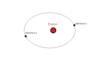
The negative hydrogen ion is a three body system of a proton and two electrons where one electron is weakly attached to the nucleus. The structure of $H^{-}$ ion is shown in Fig. 1. One of the electrons is closer to the nucleus due to repulsion from another electron. Thus, the ”inner” electron feels more charge than unity and the ”outer” electron feels less charge than unity. None of the electrons can remain at the same radial distance from the nucleus due to Coloumb repulsion. It has an early history of theoretical research. It attracted attention as an application of quantum mechanics to a two electron system during the early development of quantum mechanics. It has an astrophysical importance as it is found in stars because of the presence of hydrogen and low energy electrons that can form a bound structure when an electron comes in the vicinity of the hydrogen atom qH_RauJAA1996 . The main source of opacity in the atmosphere of the Sun at red and infrared wavelengths was predicted due to the absorption by $H^{-}$ ion qH_WildtAJ1939 . At that time it was surprising that a system such as $H^{-}$, earlier believed to be unstable before the discovery of it’s bound state could be a part of the solar spectrum, essential to sustain life on earth. It was discovered by G. Patrick Flanagan in 1983 to be present in the living fluids of all living organisms. There is very little dissociated hydrogen on earth and atmosphere. It’s spectrum corresponds to infrared and visible wavelengths. Attempts were made to calculate the ground state energy of $H^{-}$ using perturbation and variational methods but these methods failed. The energy was calculated to be -0.375 Hartree which is greater than the ground state energy of hydrogen atom (-0.5 Hartree). To prove that it is a bound state the energy must be less than that of hydrogen atom. The dynamics of the system is such that it breaks up into proton + electron + electron at infinity when it reaches 2-3 eV above the threshold energy qH_RauJAA1996 . Thus, it becomes important to consider the electron-electron correlations. The wavefunction should describe the correlations efficiently in order to get a good measure of ground state energy.

$H^{-}$ was proved as a bound entity by Bethe in 1929 using Hylleraas wavefunction qH_BetheZphys1929 . The ground state energy was further improved by Chandrasekhar qH_ChandrasekharAPJ1944 by introducing a wavefunction of the following form,

$$\psi(r1,r2)=e^{-ar_{1}-br_{2}}+e^{-br_{1}-ar_{2}}$$ (1)

where a and b are variational parameters, representing the effective nuclear charges of the electrons. This wavefunction considers electron-electron correlation implicitly. The energy was found to be -0.51330 Hartree. A much better value was calculated by Chandrasekhar when he introduced electron-electron correlation explicitly in the improved wavefunction,

$$\psi=\psi(r_{1},r_{2})(1+cr_{12})$$ (2)

where c is the new variational parameter. The energy was found to be -0.52592 Hartree. Solving the Schrodinger using trial wavefunctions is a tedious task and becomes very complicated for multi-body systems because of the difficulty to guess the wavefunction that describes the system exactly. This difficulty can be addressed by quantum computers, which have been used for the simulation of various physical systems. The largest molecule to be simulated is $H_{2}O$ qH_TengarXiv2019 . This was done by using variational quantum eigensolver that is used to find eigenvalues of a matrix qH_PeruzzoNatComm2014 ; qH_GuzikNJP2016 ; qH_GuzikarXiv2019 . VQE is better than other quantum algorithms such as phase estimation due to it’s high fidelity, robustness to errors and less resource requirement. It is based on the variational principle,

$$\frac{|\langle\psi|H|\psi\rangle|}{|\langle\psi|\psi\rangle|}\geq E$$ (3)

where E is the minimum energy eigenvalue. The variational principle ensures that this expectation value is always greater than the smallest eigenvalue of H. Here, we report the calculation of the ground state energy of $H^{-}$ ion using VQE.

II Results

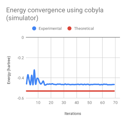
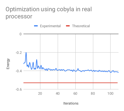
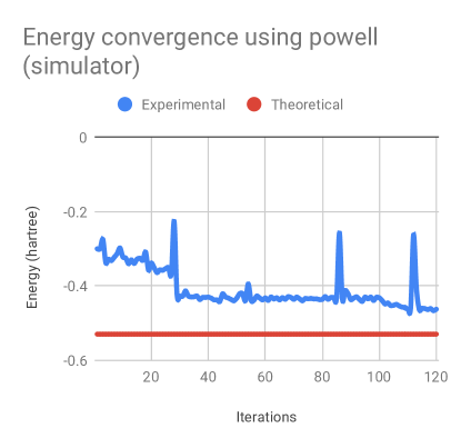
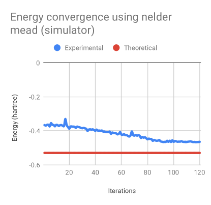
The graphical representations of the results using various optimization methods obtained using QISKit are shown.

(a) (b)

Figure 2: Energy optimization using Cobyla in QISKit aqua using ibmqx2 processor. Gate depth is 3. The red line is the theoretical value of energy calculated from Chandrasekhar wavefunction which is -0.52952. Figures (a) and (b) show the results obtained from simulator and real device respectively.

(c) (d)

Figure 3: Simulation results of energy optimization using Powell (c) and Nelder Mead (d) in QISKit aqua. Gate depth is 3. The red line is the theoretical value of energy calculated from Chandrasekhar wavefunction which is 0.52952.

The results are better than that calculated from the Hartree fock method (-0.375 Hartree). They converge to -0.468070601028 for Cobyla (simulator), -0.407087502741 for Cobyla (real processor, ibmqx2), -0.46513997401 using Powell (simulator) and -0.467324316239 for Nelder-Mead (simulator). The results do not confirm the stability of $H^{-}$ as they are still greater than the ground state energy of hydrogen atom (-0.5 Hartree). We run the VQE circuit in QISKit and calculate the expectation value of $Z_{0}I$ term. We use the same parameters of state preparation at which $Z_{0}I$ converged to calculate the expectation value of $IZ_{1}$ and $Z_{0}Z_{1}$. The probability of finding the electron in the first state is maximum. Thus, the lowest eigenvalue should be found using the set of parameters for which $Z_{0}I$ converges. Using Bravyi-Kitaev and Jordan-Wigner encoding the energy converged to -0.499711186 and -0.5339355468 (simulator) respectively much close to the theoretical value with an error of 0.8376%. The energy converged to a lower value than the theoretical value but it is within the error bound. The details of the QISKit codes with results and experimental data are provided in the Supplementary information.

Run results obtained from ibmqx2 and ibmqx4 using different sets of parameters are given below.

Figure 4: Initial rotations of the parameters of 1st and 2nd Qubit are set to $\pi/2$ and final rotations are set to 0. Gate depth is 1. Number of shots = 8192

Figure 5: Initial and final rotations of the parameters in 1st and 2nd Qubit are set to $\pi$. Gate depth is 1. Number of shots = 8192

Figure 6: Initial rotations of the parameters of 1st and 2nd Qubit are set to $\pi$ and final rotations are set to 0. Gate depth is 1. Number of shots = 8192

Figure 7: Parameters of both 1st and 2nd Qubit are set to $\pi$. Gate depth is 1. Number of shots = 8192

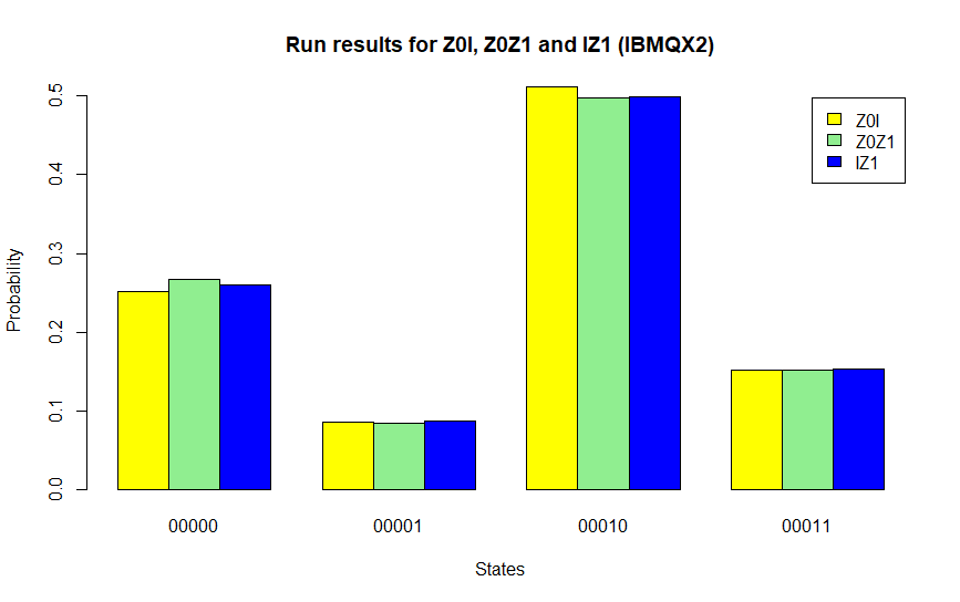
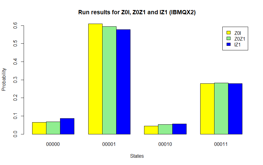
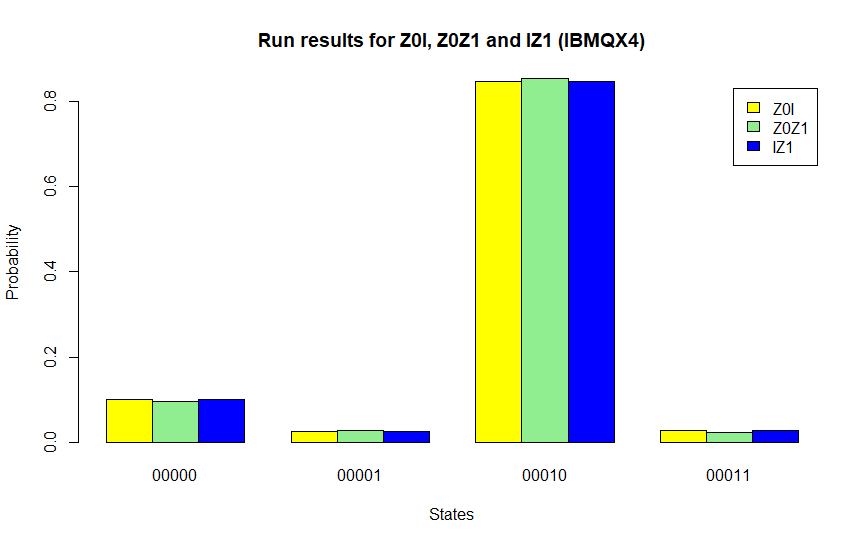
The run results (Fig.4) are obtained using ibmqx2. Initial rotations were set to $\pi/2$ and final rotations to 0 and we get the energy value -0.381156 Hartree. Setting initial and final rotations in both the qubits to $\pi$ (Fig.5), we get the energy value -0.396531 Hartree. Setting initial rotations to $\pi$ and final rotations to 0 in both qubits (Fig.6, gives the energy value -0.507891 Hartree. Using ibmqx4, when the initial and final parameters in 1st and 2nd qubit are set to $\pi$ and 0 respectively we get the energy value -0.450297.

The energy value -0.507891 Hartree is lower than that of Hydrogen atom and thus confirms the bound state of $H^{-}$ ion.

II.1 Variance

We calculate the variance for the run result -0.507891 Hartree(ibmqx2)

$$Var(H)={|\langle\psi|H^{2}|\psi\rangle|}-{|\langle\psi|H|\psi\rangle|}^{2}$$ (4)

• We first measure the variance of individual Pauli operators.

• The variance of the individual Pauli operators are then plucked in the above equation to obtain the variance.

The variance of individual Pauli operators is

$$|\langle\psi|\Delta P_{i}^{2}|\psi\rangle|=\sum_{i}({|\langle\psi|P_{i}^{2}|\psi\rangle|}-{|\langle\psi|P_{i}|\psi\rangle|}^{2})$$ (5)

where $P_{i}$’s are individual Pauli operators. Eq.4 becomes

$$Var(H)=\sum_{ij}h_{ij}^{2}(\Delta P_{i}^{2})=0.0870538$$ (6)

II.2 Conclusion

Optimization of the VQE circuit using SciPy (Python module) produced good run results but insufficient to account for the bound state of $H^{-}$. This can be attributed to the possibility of energy convergance at a local minima. Run result of the VQE cirquit in the IBM Q Experience gave the energy value -0.507891 Hartree with an error of 3.3 % from the theoretical value obtained using Chandrasekhar wavefunction. The entangled state of two electron system (correlated wavefunction of $H^{-}$) is efficiently realized in the IBM Quantum Computer.

Materials and Method

III The Second-Quantized Hamiltonian

The second quantized Hamiltonian for fermions is given by,

$$H=\sum_{i,j}h_{ij}a_{i}^{\dagger}a_{j}+\frac{1}{2}\sum_{i,j,k,l}h_{ijkl}a_{i}^{\dagger}a_{j}^{\dagger}a_{k}a_{l}$$ (7)

where $h_{ij}$ and $h_{ijkl}$ are one and two electron integrals given by

$$h_{ij}=\int d\vec{r_{1}}\chi_{i}^{*}(\vec{r_{1}})(\frac{-\nabla_{1}^{2}}{2}-{\sum_{\sigma}\frac{Z}{|\vec{r_{1}}\ -R_{\sigma}|}})\chi_{j}(\vec{r_{1}})$$ (8)

and

$$h_{ijkl}=\int\frac{d\vec{r_{1}}d\vec{r_{2}}\chi_{i}^{*}(\vec{r_{1}})\chi_{j}^{*}(\vec{r_{2}})}{|(r_{1}-r_{2})|}\frac{{\chi_{k}(\vec{r_{2}})}{\chi_{l}(\vec{r_{1}})}}{2}$$ (9)

where ${\chi_{i}(\vec{r_{1}})}$ is the $i$th spin orbital, Z is the nuclear charge, ${\vec{r_{i}}}$ is the position of the $i$th electron, $r_{12}$ is the distance between the two points $r_{1}$ and $r_{2}$. $R_{\sigma}$ is the position of the nucleus. $a_{i}^{\dagger}$ and $a_{j}$ are fermionic creation and annihillation operators that follow the anti-commutation relations,

$$\{a_{i}^{\dagger},a_{j}\}=\delta_{ij}$$ (10)

$$\{a_{i},a_{j}\}=0$$ (11)

The fermionic creation operator increases the occupational number of an orbital by one and the annihilation operator decreases it by one. Using Jordan-Wigner or Bravyi-Kitaev transform, the fermionic Hamiltonian can be mapped to spin type Hamiltonian.

IV The Jordan-Wigner transform

Jordan-Wigner transform is a second-quantized encoding method to encode fermions into qubits. The mapping qH_bravyi2012 is given by,

$$a{{}_{i}}=Q{{}_{i}}{\otimes}Z{{}_{i-1}}{\otimes}Z{{}_{i-2}}....{\otimes}Z{{}_{0}}$$ (12)

$$a_{i}^{\dagger}=Q^{\dagger}{\otimes}Z{{}_{i-1}}{\otimes}Z{{}_{i-2}}....{\otimes}Z{{}_{0}}$$ (13)

where,

$$Q=\frac{X+iY}{2}$$ (14)

$$Q{{}^{\dagger}}=\frac{X-iY}{2}$$ (15)

Each qubit stores the occupation number of the orbital.

V The Parity Transformation

In the parity basis the qubit stores the parity of all occupied orbitals qH_bravyi2012 . The mapping is given by, $p_{i}$ = $\sum_{j}[\pi_{n}]_{ij}f_{j}$. This changes the occupation number basis state to it’s corresponding parity basis state. The matrix form of $[\pi_{n}]_{ij}$ is given by,

$$\begin{split}\left[{\begin{array}[]{cccc}1&0&0&0\\ 1&1&0&0\\ 1&1&1&0\\ 1&1&1&1\\ \end{array}}\right]\end{split}$$

VI The Bravyi Kitaev Transform

The Bravyi Kitaev Transform is a midway between the Jordan Wigner and parity encoding. The orbitals store partial sums of occupation numbers qH_GuzikarXiv2019 . The qubit stores the parity of the set of occupation numbers corresponding to that set of orbitals. The qubits store occupation numbers when indices are even and parity when indices are odd. The transformation qH_bravyi2012 is given by, $b_{i}$ = $\sum_{j}[\beta_{n}]_{ij}f_{j}$, the matrix $[\beta_{n}]_{ij}$ for a 4 qubit system is,

$$\begin{split}\left[{\begin{array}[]{cccc}1&0&0&0\\ 1&1&0&0\\ 0&0&1&0\\ 1&1&1&1\\ \end{array}}\right]\end{split}$$

The relation of creation and annihilation operators qH_bravyi2012 is given by,

$$a_{i}^{\dagger}=X_{U(i)}Q_{i}^{\dagger}{\otimes}Z_{p(i)}$$ (16)

$$a_{i}=X_{U(i)}Q_{i}^{\dagger}{\otimes}Z_{p(i)}$$ (17)

VII Hamiltonian of the $H^{-}$ ion

The $H^{-}$ ion consists of two electrons, one of which is closer to the nucleus (Fig. 1). Thus, it has two states with one electron each. Thus the Hamiltonian given in Eq. (7) can be expanded using the Jordan-Wigner transform as qH_GuzikarXiv2019 ,

$$H =h_{00}(a_{0}^{\dagger}a_{0})+h_{11}(a_{1}^{\dagger}a_{1})+\frac{1}{2}h_{0101}(a_{0}^{\dagger}a_{1}^{\dagger}a_{0}a_{1})$$ (18)

$$+\frac{1}{2}h_{0110}(a_{0}^{\dagger}a_{1}^{\dagger}a_{1}a_{0})+\frac{1}{2}h_{1001}(a_{1}^{\dagger}a_{0}^{\dagger}a_{0}a_{1})$$

$$+\frac{1}{2}h_{1010}(a_{1}^{\dagger}a_{0}^{\dagger}a_{1}a_{0})$$

Using the anti-commutation relations (10) and (11), the Hamiltonian becomes,

$$H =h_{00}(a_{0}^{\dagger}a_{0})+h_{11}(a_{1}^{\dagger}a_{1})+h_{0101}(a_{0}^{\dagger}a_{1}^{\dagger}a_{0}a_{1})$$ (19)

$$+h_{0110}(a_{1}^{\dagger}a_{0}^{\dagger}a_{0}a_{1})$$

where we have used the fact that, $h_{0101}=h_{1010}$ and $h_{0110}=h_{1010}$. Using J-W transform (13), we have,

$$a_{0}^{\dagger}a_{0}=Q_{0}^{\dagger}Q_{0},$$

$$a_{1}^{\dagger}a_{1}=(Q_{1}^{\dagger}{\otimes}Z_{0})(Q_{1}{\otimes}Z_{0}),$$

$$a_{0}^{\dagger}a_{1}^{\dagger}a_{0}a_{1}=(Q_{0}^{\dagger})(Q_{1}^{\dagger}{\otimes}Z_{0})(Q_{0})(Q_{1}{\otimes}Z_{0}),$$

$$a_{1}^{\dagger}a_{0}^{\dagger}a_{0}a_{1}=(Q_{1}^{\dagger}{\otimes}Z_{0})(Z_{0})(Z_{0})(Q_{1}{\otimes}Z_{0})$$ (20)

Making use of the tensor product relation $(A{\otimes}B)(C{\otimes}D)=(AC){\otimes}(BD)$, The Hamiltonian simplifies to,

$$H =\frac{1}{2}h_{00}{(1-Z_{0})}+\frac{1}{2}h_{11}{(1-Z_{1})}$$ (21)

$$+\frac{1}{8}h_{0110}{(1-Z_{0}-Z_{1}+{Z_{0}}{\cdot Z_{1})}}$$

Similarly using Bravyi-Kitaev transform the Hamiltonian for $H^{-}$ is

$$H =\frac{1}{2}h_{00}{(1-Z_{0})}+\frac{1}{2}h_{11}{(1-Z_{1}Z_{0})}$$ (22)

$$+\frac{1}{8}h_{0110}{(1-Z_{0}+Z_{1}-{Z_{0}}{\cdot Z_{1})}}$$

VIII Method of Simulation

The method of simulation consists of 2 parts,

Quantum

• Prepare the state ${\psi}$, also known as the ansatz.

• Measure the expectation value ${|\langle\psi|H|\psi\rangle|}$ using algorithms such as phase estimation or variational quantum eigensolver.

Classical

• Use a classical optimizer such as Nelder-Mead, Powell, Coybala and gradient descent methods for optimization.

• Iterate until the energy converges.

VIII.1 Variational Quantum Eigensolver

The quantum part of simulation is performed using variational quantum eigensolver as the algorithm to run the quantum subroutine. VQE was first demonstrated in 2014 qH_PeruzzoNatComm2014 . It has also been demonstrated in the Refs. qH_LeiWangarXiv2019 ; qH_MartinezarXiv2019 ; qH_CollessPRL2018 . The state preparation is done by entangling the qubits using various single qubit rotation gates to produce a complex state. VQE is capable of finding the ground state energies of small molecules using low depth circuits. It is based on the Rayleigh-Ritz variational principle,

$${|\langle\psi({\theta_{i}})|H|\psi({\theta_{i}})\rangle|}\geq E_{0}.$$ (23)

where $E_{0}$ is the ground state energy. The wave function is taken to be normalized. The circuit diagram of VQE qH_TengarXiv2019 for gate depth 1 is shown in Fig. 8. The circuit consists of 2 parts,

Initial state preparation (ansatz) -

• The two qubit system is given initial rotations using the gates $U_{0}$ and $U_{1}$ followed by $CNOT$s. The unitary gates $U_{i}$ are of the form $R_{z}({\theta_{i}})R_{x}({\theta_{i}})R_{z}({\theta_{i}})$. The parameters ${\theta_{i}}$ have to be adjusted. This completes one layer of entanglement. The layers can be increased to produce more complex state as required. For an n-qubit system, the number of parameters for initial rotations would be 3n(n-1) and the number of unitary gates required is given n(n-1) qH_TengarXiv2019 . For a two-qubit system, we thus need six parameters and two unitary gates. It is then followed by final rotations $U_{2}$ and $U_{3}$.

Measurement

• The expectation values of each term in the Hamiltonian is measured one by one by introducing each Pauli term in the circuit after the state preparation as shown in Fig. 8.

VIII.2 Optimization for Energy Convergence

Optimization (classical part) is the last step for finding the minimum (ground state) energy. There are various optimization methods classified into two categories qH_GuzikarXiv2019 ,

Direct Search Method

Direct search algorithms do not make use of the gradient of the objective function e.g., particle swarm optimization, Nelder-Mead, Powell and Cobyla. These methods have been proven to be much better than gradient-based method. Nelder Mead is a good method for optimization. It is used in the fields of chemistry, medicine, science and technology. The method is derivative free and is used in systems where the functions are noisy and discontinuous such as parameter estimation and statistical problems. Powell method requires repeated line search minimization, which may be carried out using univariate gradient free, or gradient-based procedures. Cobyla constructs successive linear approximations of the objective function and constraints via a simplex of n+1 points (in n dimensions), and optimizes these approximations in a trust region at each step.

Gradient-based Method Gradient-based methods use the gradient of the objective function. Examples are simultaneous perturbation stochastic approximation (SPSA) algorithm, and L-BFGS-B. SPSA calculates the gradient by,

$$G(\theta) =\frac{1}{2}({\langle\psi({\theta_{i}+{\pi/2}})|H|\psi({\theta_{i}+{\pi/2}}\rangle})$$ (24)

$$-{|\langle\psi({\theta_{i}-{\pi/2}})|H|\psi({\theta_{i}-{\pi/2}}\rangle})$$

where $G({\theta}$ is the gradient. The parameters are then updated according to whether the gradient decreases or increases. L-BFGS-B minimizes a differentiable scalar function f(x) over unconstrained values of the real-vector “x” qH_Malou2002 . Gradient-based optimization converges the function to a local minima, thus giving poor results. They are not used for functions with large number of parameters. Direct methods are much efficient and provide good values. But they are dependent on the system. Results vary with the number of qubits and gate depth. Here, we use Nelder-Mead, Cobyla and Powell methods and compare the results to depict which method is best suited for the calculation of ground state energy of $H^{-}$.

Figure 8: Quantum circuit illustrating the variational quantum eigensolver for two-qubit system. The unitary operations $U_{0}$, $U_{1}$ and two $CNOT$ gates are used to create entanglement in the system for initial state preparation. $U_{2}$ and $U_{3}$ are then applied on the qubits $q_{0}$ and $q_{1}$ respectively for final rotations. Finally the terms of the Hamiltonian (Pauli matrices) are applied to calculate their expectation values.

VIII.3 Implementation

In order to determine the ground state energy, we need the “h” values $h_{00}$, $h_{11}$ and $h_{0101}$ given in Eq. (VII). The “h” values are calculated by solving the one electron integrals (Eqs. (8) and (9)). They have been calculated in lecture 18 of the lecture series titled “Quantum Principles” qH_Lecture182014 . They are given as, $h_{00}$ = $h_{11}$ = 0.5, $h_{0101}$ = 0.625, $h_{00}$ and $h_{11}$ are equal as electrons are fermions (identical and indistinguishable particles). The expectation value of Hamiltonian is therefore,

$$\langle\psi|H|\psi\rangle =\frac{1}{4}\langle\psi{(1-Z_{0})}\psi\rangle+\frac{1}{4}\langle\psi{(1-Z_{1})}\psi\rangle$$ (25)

$$+\frac{5}{64}\langle\psi{(1-Z_{0}-Z_{1}-{Z_{0}}{\cdot Z_{1})}\psi\rangle}$$

The expectation of $Z_{0}$I, I$Z_{1}$ and $Z_{0}{{Z_{1}}}$ can be found by placing Z gates on qubits $q_{0}$ and $q_{1}$ after final rotation gates and measuring both the qubits.

In matrix form, $Z_{0}$I =

$$\begin{split}\left[{\begin{array}[]{cccc}1&0&0&0\\ 0&1&0&0\\ 0&0&-1&0\\ 0&0&0&-1\\ \end{array}}\right]\end{split}$$

the eigenvalues are

• +1 for $|00\rangle$ and $|01\rangle$

• -1 for $|10\rangle$ and $|11\rangle$

Expectation value is, $\langle\psi|Z_{0}I|\psi\rangle$ = $P_{00}$ + $P_{01}$ - $P_{10}$ - $P_{11}$, where the eigenvalues have been multiplied as coefficients with respective eigenvectors. Similarly,

I$Z_{1}$ =

$$\begin{split}\left[{\begin{array}[]{cccc}1&0&0&0\\ 0&-1&0&0\\ 0&0&1&0\\ 0&0&0&-1\\ \end{array}}\right]\end{split}$$

the eigenvalues are

• +1 for $|00\rangle$ and $|10\rangle$

• -1 for $|01\rangle$ and $|11\rangle$

$\langle\psi|IZ_{1}|\psi\rangle$ = $P_{00}$ - $P_{01}$ + $P_{10}$ - $P_{11}$ and

$Z_{0}Z_{1}$ =

$$\begin{split}\left[{\begin{array}[]{cccc}1&0&0&0\\ 0&-1&0&0\\ 0&0&-1&0\\ 0&0&0&1\\ \end{array}}\right]\end{split}$$

the eigenvalues are

• +1 for $|00\rangle$ and $|11\rangle$

• -1 for $|01\rangle$ and $|10\rangle$

$$\langle\psi|Z_{0}Z_{1}|\psi\rangle=P_{00}-P_{01}-P_{10}+P_{11}$$ (26)

The initial parameters may be chosen at random. It can be adjusted according to the measured expectation value. We depict a comparison between various optimization methods. The optimization was performed by running codes in QISKit and running program in QISKit aqua.

Data availability

Data are available to any reader upon reasonable request.

Author contributions

S.K. has done theoretical analysis and developed the protocol. S.K. and B.K.B. have analyzed and designed the quantum circuits. S.K., R.P.S. and B.K.B. have implemented the circuits on IBM quantum experience platform and performed the experiments. R.P.S. has written the circuit codes, run the optimization routine and quantum chemistry program for energy convergence in QISKit Terra and QISKit Aqua. S.K. and B.K.B. contributed to the composition of the manuscript. B.K.B has supervised the project. P.K.P. thoroughly checked and reviewed the manuscript. S.K., R.P.S. and B.K.B. have completed the project under the guidance of P.K.P.

Competing interests

The authors declare no competing financial as well as non-financial interests.

IX Supplementary Information: QISKIT codes for optimization.

For Energy estimation $Z_{0}I$, $IZ_{1}$ and $Z_{0}Z_{1}$ terms of Hamiltonian respectively are coded then optimized through scipy.optimize which contain ’powell’, ’nelder-mead’ or ’cobyla’. The QASM code for the same is as follows:
Code for Z1($Z_{0}I$):

⬇

1# -*- coding: utf-8 -*-

2”””

3Created on Wed Feb 13 20:04:16 2019

4

5@author: Rahul

6”””

7

8from scipy.optimize import minimize

9from qiskit import QuantumCircuit, ClassicalRegister, QuantumRegister

10import numpy as np

11from qiskit import execute

12from qiskit import BasicAer

13backend = BasicAer.get_backend(’qasm_simulator’)

14T=8192

15def Z1(theta):

16 # Create a Quantum Register called ”q” with 3 qubits

17 q = QuantumRegister(2)

18

19 # Create a Classical Register called ”c” with 3 bits

20 c = ClassicalRegister(2)

21 qc = QuantumCircuit(q,c)

22

23 qc.u1(theta[0],q[0])

24 qc.u3(theta[1],-np.pi/2,np.pi/2,q[0])

25 qc.u1(theta[2],q[0])

26 qc.cx(q[0], q[1])

27 qc.u1(theta[3],q[1])

28 qc.u3(theta[4],-np.pi/2,np.pi/2,q[1])

29 qc.u1(theta[5],q[1])

30 qc.cx(q[1], q[0])

31 qc.u1(theta[6],q[0])

32 qc.u1(theta[7],q[1])

33 qc.u3(theta[8],-np.pi/2,np.pi/2,q[0])

34 qc.u3(theta[9],-np.pi/2,np.pi/2,q[1])

35 qc.u1(theta[10],q[0])

36 qc.u1(theta[11],q[1])

37 qc.z(q[0])

38

39 qc.measure(q[0], c[0])

40 qc.measure(q[1], c[1])

41

42 #print(qc)

43 #print(i)

44 shots = T # Number of shots to run the program (experiment); maximum is 8192 shots.

45 max_credits = 3 # Maximum number of credits to spend on executions.

46

47 job_hpc = execute(qc, backend=backend, shots=shots, max_credits=max_credits)

48 result_hpc = job_hpc.result()

49 counts11 = result_hpc.get_counts(qc)

50 #print(counts11)

51 Z=0

52 if ’00’ in list(counts11):

53 Z=Z+counts11[’00’]/T

54 #print(Z)

55 if ’01’ in list(counts11):

56 Z=Z+counts11[’01’]/T

57 #print(Z)

58 if ’10’ in list(counts11):

59 Z=Z-counts11[’10’]/T

60 #print(Z)

61 if ’11’ in list(counts11):

62 Z=Z-counts11[’11’]/T

63 #print(Z)

64

65 return Z

66theta0=[0,np.pi/2,0,0,np.pi/2,0,0,0,np.pi/2,np.pi/2,0,0]

67res = minimize(Z1, theta0, method=’powell’,options={’xtol’: 1e-8 , ’disp’: True})

68print(res,’Z1’)

69#x=Z1([ 1.53637770e-03, 1.55027283e+00, 8.09473120e-04, 1.66340534e-04,-8.32420733e-03, -2.28166637e-05, -8.94140209e-04, 5.61023344e-04,1.77675920e+00, 1.58425510e+00, 1.09455026e-03, 8.51956374e-04])

70#print(x)

Code for Z2($IZ_{1}$):

⬇

1# -*- coding: utf-8 -*-

2”””

3Created on Wed Feb 13 20:04:17 2019

4

5@author: Rahul

6”””

7

8from scipy.optimize import minimize

9from qiskit import QuantumCircuit, ClassicalRegister, QuantumRegister

10import numpy as np

11from qiskit import execute

12from qiskit import BasicAer

13backend = BasicAer.get_backend(’qasm_simulator’)

14T=8192

15def Z2(theta):

16 # Create a Quantum Register called ”q” with 3 qubits

17 q = QuantumRegister(2)

18

19 # Create a Classical Register called ”c” with 3 bits

20 c = ClassicalRegister(2)

21 qc = QuantumCircuit(q,c)

22

23 qc.u1(theta[0],q[0])

24 qc.u3(theta[1],-np.pi/2,np.pi/2,q[0])

25 qc.u1(theta[2],q[0])

26 qc.cx(q[0], q[1])

27 qc.u1(theta[3],q[1])

28 qc.u3(theta[4],-np.pi/2,np.pi/2,q[1])

29 qc.u1(theta[5],q[1])

30 qc.cx(q[1], q[0])

31 qc.u1(theta[6],q[0])

32 qc.u1(theta[7],q[1])

33 qc.u3(theta[8],-np.pi/2,np.pi/2,q[0])

34 qc.u3(theta[9],-np.pi/2,np.pi/2,q[1])

35 qc.u1(theta[10],q[0])

36 qc.u1(theta[11],q[1])

37 qc.z(q[1])

38

39 qc.measure(q[0], c[0])

40 qc.measure(q[1], c[1])

41

42 #print(qc)

43 #print(i)

44 shots = T # Number of shots to run the program (experiment); maximum is 8192 shots.

45 max_credits = 3 # Maximum number of credits to spend on executions.

46

47 job_hpc = execute(qc, backend=backend, shots=shots, max_credits=max_credits)

48 result_hpc = job_hpc.result()

49 counts22 = result_hpc.get_counts(qc)

50

51 Z=0

52 if ’00’ in list(counts22):

53 Z=Z+counts22[’00’]/T

54 print(Z)

55 if ’01’ in list(counts22):

56 Z=Z-counts22[’01’]/T

57 print(Z)

58 if ’10’ in list(counts22):

59 Z=Z+counts22[’10’]/T

60 print(Z)

61 if ’11’ in list(counts22):

62 Z=Z-counts22[’11’]/T

63 print(Z)

64

65 return Z

66theta0=[0,np.pi/2,0,0,np.pi/2,0,0,0,np.pi/2,np.pi/2,0,0]

67res = minimize(Z2, theta0, method=’nelder-mead’,options={’xtol’: 1e-8 , ’disp’: True})

68print(res,’Z2’)

69#z=Z2([-5.64200351e-01, 1.61554986e+00, 1.56821823e+00, 1.61219634e-03, 1.81902336e+00, 5.96777406e+00, -6.66574506e-03, 4.63725496e+00, 1.32156756e+00, 3.78827977e-01, 9.59049221e+00, 3.90466495e+00])

70#print(z)

Code for Z3($Z_{0}Z_{I}$):

⬇

1# -*- coding: utf-8 -*-

2”””

3Created on Wed Feb 13 20:04:15 2019

4

5@author: Rahul

6”””

7

8from scipy.optimize import minimize

9from qiskit import QuantumCircuit, ClassicalRegister, QuantumRegister

10import numpy as np

11from qiskit import execute

12from qiskit import IBMQ

13backend =IBMQ.get_backend(’ibmqx4’)

14T=8192

15def Z3(theta):

16 # Create a Quantum Register called ”q” with 3 qubits

17 q = QuantumRegister(2)

18

19 # Create a Classical Register called ”c” with 3 bits

20 c = ClassicalRegister(2)

21 qc = QuantumCircuit(q,c)

22

23 qc.u1(theta[0],q[0])

24 qc.u3(theta[1],-np.pi/2,np.pi/2,q[0])

25 qc.u1(theta[2],q[0])

26 qc.cx(q[0], q[1])

27 qc.u1(theta[3],q[1])

28 qc.u3(theta[4],-np.pi/2,np.pi/2,q[1])

29 qc.u1(theta[5],q[1])

30 qc.cx(q[1], q[0])

31 qc.u1(theta[6],q[0])

32 qc.u1(theta[7],q[1])

33 qc.u3(theta[8],-np.pi/2,np.pi/2,q[0])

34 qc.u3(theta[9],-np.pi/2,np.pi/2,q[1])

35 qc.u1(theta[10],q[0])

36 qc.u1(theta[11],q[1])

37 qc.z(q[0])

38 qc.z(q[1])

39

40 qc.measure(q[0], c[0])

41 qc.measure(q[1], c[1])

42

43 #print(qc)

44 #print(i)

45 shots= T # Number of shots to run the program (experiment); maximum is 8192 shots.

46 max_credits = 3 # Maximum number of credits to spend on executions.

47

48 job_hpc = execute(qc, backend=backend, shots=shots, max_credits=max_credits)

49 result_hpc = job_hpc.result()

50 counts12 = result_hpc.get_counts(qc)

51

52 Z=0

53 if ’00’ in list(counts12):

54 Z=counts12[’00’]/T

55 print(Z)

56 if ’01’ in list(counts12):

57 Z=Z-counts12[’01’]/T

58 print(Z)

59 if ’10’ in list(counts12):

60 Z=Z-counts12[’10’]/T

61 print(Z)

62 if ’11’ in list(counts12):

63 Z=Z+counts12[’11’]/T

64 print(Z)

65 return Z

66theta0=[0,np.pi/2,0,0,np.pi/2,0,0,0,np.pi/2,np.pi/2,0,0]

67res = minimize(Z3, theta0, method=’nelder-mead’,options={’xtol’: 1e-8 , ’disp’: True})

68print(res,’Z3’)

69#y=Z3([-7.63609374, -0.31633082, 2.15909817, 4.31092763, 1.57470161, 1.6111563 , -0.13041641, 0.08880943, 1.58865914, 1.50475982, 0.59323763, 2.86816974])

70#print(y)

The tabulated data of convergence is as shown below.

Table 1: For Nelder Mead

Iterations	Theoretical	Experimental
1	-0.52952	-0.3658118514
2	-0.52952	-0.3687388385
3	-0.52952	-0.364456499
4	-0.52952	-0.3640980715
5	-0.52952	-0.3735459878
6	-0.52952	-0.3547868431
7	-0.52952	-0.3642996161
8	-0.52952	-0.3652836663
9	-0.52952	-0.3730938032
10	-0.52952	-0.3646086323
11	-0.52952	-0.3657974241
12	-0.52952	-0.3712501318
13	-0.52952	-0.3667064972
14	-0.52952	-0.3660282661
15	-0.52952	-0.3702449038
16	-0.52952	-0.3702913827
17	-0.52952	-0.3308180563
18	-0.52952	-0.3653252632
19	-0.52952	-0.3770401351
20	-0.52952	-0.3867578684
21	-0.52952	-0.3746037324
22	-0.52952	-0.3745729229
23	-0.52952	-0.375111539
24	-0.52952	-0.3759054584
25	-0.52952	-0.3819807294
26	-0.52952	-0.3751555337
27	-0.52952	-0.3774191599
28	-0.52952	-0.3790968918
29	-0.52952	-0.3830969824
30	-0.52952	-0.3842554535
31	-0.52952	-0.3821377446
32	-0.52952	-0.3852416368
33	-0.52952	-0.387955228
34	-0.52952	-0.3997053027
35	-0.52952	-0.3925481822
36	-0.52952	-0.3912610618
37	-0.52952	-0.3925515116
38	-0.52952	-0.39142132
39	-0.52952	-0.3948359592
40	-0.52952	-0.3993956196
41	-0.52952	-0.3929185069
42	-0.52952	-0.3984600897
43	-0.52952	-0.3981955975
44	-0.52952	-0.3995114402
45	-0.52952	-0.3982939261
46	-0.52952	-0.4039865324
47	-0.52952	-0.4040763391
48	-0.52952	-0.4061567579
49	-0.52952	-0.4068460868
50	-0.52952	-0.4075465596

Iterations	Theoretical	Experimental
51	-0.52952	-0.4042369078
52	-0.52952	-0.4167492066
53	-0.52952	-0.4100107529
54	-0.52952	-0.4121749407
55	-0.52952	-0.4123393275
56	-0.52952	-0.4153778284
57	-0.52952	-0.4201981629
58	-0.52952	-0.416993412
59	-0.52952	-0.4075684502
60	-0.52952	-0.4216554432
61	-0.52952	-0.4229979668
62	-0.52952	-0.4196147123
63	-0.52952	-0.4253503764
64	-0.52952	-0.4249917301
65	-0.52952	-0.4299162527
66	-0.52952	-0.4330937475
67	-0.52952	-0.4257880472
68	-0.52952	-0.4038551852
69	-0.52952	-0.424561212
70	-0.52952	-0.4276609296
71	-0.52952	-0.4244919108
72	-0.52952	-0.4281787243
73	-0.52952	-0.4255140557
74	-0.52952	-0.4291707672
75	-0.52952	-0.4413052833
76	-0.52952	-0.4357576628
77	-0.52952	-0.4398903991
78	-0.52952	-0.4376459041
79	-0.52952	-0.4434627664
80	-0.52952	-0.4494898276
81	-0.52952	-0.445895972
82	-0.52952	-0.4480489295
83	-0.52952	-0.448329137
84	-0.52952	-0.4582959119
85	-0.52952	-0.4535441657
86	-0.52952	-0.4562919823
87	-0.52952	-0.458321483
88	-0.52952	-0.4572042524
89	-0.52952	-0.4542379797
90	-0.52952	-0.4615284535
91	-0.52952	-0.4637654447
92	-0.52952	-0.4654706567
93	-0.52952	-0.4647630364
94	-0.52952	-0.4646672379
95	-0.52952	-0.4587078335
96	-0.52952	-0.4644073631
97	-0.52952	-0.458071464
98	-0.52952	-0.4648104928
99	-0.52952	-0.455790524
100	-0.52952	-0.4643548465

Iterations	Theoretical	Experimental
101	-0.52952	-0.4597123945
102	-0.52952	-0.4614880122
103	-0.52952	-0.4640232781
104	-0.52952	-0.4631510063
105	-0.52952	-0.4633038065
106	-0.52952	-0.4607956644
107	-0.52952	-0.4640445423
108	-0.52952	-0.4648928415
109	-0.52952	-0.464328522
109	-0.52952	-0.4654582708
110	-0.52952	-0.4653556353
111	-0.52952	-0.4637653123
112	-0.52952	-0.4627551564
113	-0.52952	-0.4616840943
114	-0.52952	-0.4639483874
115	-0.52952	-0.4658633096
116	-0.52952	-0.4652171301
117	-0.52952	-0.4662359862
118	-0.52952	-0.4657969867
119	-0.52952	-0.4654209807
120	-0.52952	-0.4644860719
121	-0.52952	-0.4655182454
122	-0.52952	-0.4639068364
123	-0.52952	-0.4650023139
124	-0.52952	-0.4634304145
125	-0.52952	-0.4670682595

Table 2: For Cobyla on real Chip

Iterations	Theoretical	Experimental
1	-0.52952	-0.3242458015
2	-0.52952	-0.312141158
3	-0.52952	-0.3000890929
4	-0.52952	-0.2012450742
5	-0.52952	-0.3431368385
6	-0.52952	-0.3354519405
7	-0.52952	-0.3605707275
8	-0.52952	-0.3092321975
9	-0.52952	-0.3421126117
10	-0.52952	-0.382317455
11	-0.52952	-0.365973851
12	-0.52952	-0.3070352964
13	-0.52952	-0.378163368
14	-0.52952	-0.372308508
15	-0.52952	-0.3760271897
16	-0.52952	-0.2783118205
17	-0.52952	-0.3703690787
18	-0.52952	-0.3461754311
19	-0.52952	-0.3659191554
20	-0.52952	-0.3757416573
21	-0.52952	-0.3401756666
22	-0.52952	-0.3805747747
23	-0.52952	-0.3638238258
24	-0.52952	-0.3789247876
25	-0.52952	-0.3807448887
26	-0.52952	-0.3913352043
27	-0.52952	-0.3779779816
28	-0.52952	-0.3963448298
29	-0.52952	-0.3759803137
30	-0.52952	-0.3827794955
31	-0.52952	-0.3805431712
32	-0.52952	-0.3928037149
33	-0.52952	-0.385364926
34	-0.52952	-0.3918327581
35	-0.52952	-0.3848496156
36	-0.52952	-0.3892537216
37	-0.52952	-0.3883246723
38	-0.52952	-0.3732819491
39	-0.52952	-0.3917883664
40	-0.52952	-0.3926158442
41	-0.52952	-0.3891585442
42	-0.52952	-0.3859512631
43	-0.52952	-0.3947456284
44	-0.52952	-0.3852036904
45	-0.52952	-0.3942924663
46	-0.52952	-0.3859246281
47	-0.52952	-0.3890963958
48	-0.52952	-0.4008480231
49	-0.52952	-0.4013480612
50	-0.52952	-0.3944512178

Iterations	Theoretical	Experimental
51	-0.52952	-0.3884351222
52	-0.52952	-0.3884351222
53	-0.52952	-0.3884351222
54	-0.52952	-0.3907311105
55	-0.52952	-0.3980456027
56	-0.52952	-0.3906448114
57	-0.52952	-0.4059641886
58	-0.52952	-0.388795591
59	-0.52952	-0.3965149438
60	-0.52952	-0.4046238846
61	-0.52952	-0.4025665527
62	-0.52952	-0.3938826373
63	-0.52952	-0.3762519993
64	-0.52952	-0.395794006
65	-0.52952	-0.3963359515
66	-0.52952	-0.4041835107
67	-0.52952	-0.4079657663
68	-0.52952	-0.3994302984
69	-0.52952	-0.3969173201
70	-0.52952	-0.4045947654
71	-0.52952	-0.3955795003
72	-0.52952	-0.396464158
73	-0.52952	-0.3954576879
74	-0.52952	-0.3922859202
75	-0.52952	-0.3903440066
76	-0.52952	-0.3997641322
77	-0.52952	-0.3953649947
78	-0.52952	-0.3912133919
79	-0.52952	-0.4025246453
80	-0.52952	-0.4028140875
81	-0.52952	-0.3936148616
82	-0.52952	-0.4070786244
83	-0.52952	-0.3972980299
84	-0.52952	-0.401852009
85	-0.52952	-0.4013366986
86	-0.52952	-0.4078261972
87	-0.52952	-0.3935246526
88	-0.52952	-0.4035197528
89	-0.52952	-0.4009673514
90	-0.52952	-0.4068310896
91	-0.52952	-0.4011399496
92	-0.52952	-0.407983523
93	-0.52952	-0.4008302665
94	-0.52952	-0.4089342389
95	-0.52952	-0.404329474
96	-0.52952	-0.4098480158
97	-0.52952	-0.4068971478
98	-0.52952	-0.3970568892
99	-0.52952	-0.4050681684
100	-0.52952	-0.4176714243

Iterations	Theoretical	Experimental
101	-0.52952	-0.4127125846
102	-0.52952	-0.4028407225
103	-0.52952	-0.397501173
104	-0.52952	-0.4120374641
105	-0.52952	-0.4085077118
106	-0.52952	-0.4095649677
107	-0.52952	-0.4097617167
108	-0.52952	-0.4122036682
109	-0.52952	-0.4182641555

References

- (1) S. Chandrasekhar, Some Remarks on the Negative Hydrogen Ion and Its Absorption Coefficient, Astrophys. J. 100, 176 (1944).
- (2) A. Peruzzo, J. McClean, P. Shadbolt, M.-H. Yung, X.-Q. Zhou, P. J. Love, A. Aspuru-Guzik, and J. L. O’Brien, A variational eigenvalue solver on a quantum processor, Nat. Commun. 5, 4213 (2014).
- (3) A. Kandala, A. Mezzacapo, K. Temme, M. Takita, M. Brink, J. M. Chow, and J. M. Gambetta, Hardware-efficient Variational Quantum Eigensolver for Small Molecules and Quantum Magnets, Nature 549, 242 (2017).
- (4) S. Wiesner, Simulations of Many-Body Quantum Systems by a Quantum Computer, arXiv:quant-ph/9603028.
- (5) I. M. Georgescu, S. Ashhab, and F. Nori, Rev. Mod. Phys. 86, 153 (2014).
- (6) R. P. Feynman, Simulating Physics with Computers, Int. J. Theor. Phys. 21, 467 (1982).
- (7) S. Lloyd, Universal Quantum Simulators, Science 273, 1073 (1996).
- (8) S. Sachdev, Quantum Phase Transitions, Cambridge University Press, Cambridge, U.K. (1999).
- (9) S. Sachdev, Quantum magnetism and criticality, Nat. Phys. 4, 173 (2008).
- (10) B. P. Lanyon, J. D. Whitfield, G. G. Gillett, M. E. Goggin, M. P. Almeida, I. Kassal, J. D. Biamonte, M. Mohseni, B. J. Powell, M. Barbieri, A. Aspuru-Guzik, and A. G. White, Towards quantum chemistry on a quantum computer, Nat. Chem. 2, 106 (2010).
- (11) E. F. Dumitrescu, A. J. McCaskey, G. Hagen, G. R. Jansen, T. D. Morris, T. Papenbrock, R. C. Pooser, D. J. Dean, and P. Lougovski, Phys. Rev. Lett. 120, 210501 (2018).
- (12) N. Lambert, Y.-N. Chen, Y.-C. Cheng, C.-M. Li, G.-Y. Chen, and F. Nori, Quantum biology, Nat. Phys. 9, 10 (2013).
- (13) S. Lloyd, A theory of quantum gravity based on quantum computation, arXiv:quant-ph/0501135.
- (14) P. A. Zizzi, Quantum Computation Toward Quantum Gravity, Gen. Relat. Gravit. 33, 1305 (2001).
- (15) A. Trabesinger, Quantum simulation, Nat. Phys. 8, 263 (2012).
- (16) J. I. Cirac and P. Zoller, Goals and opportunities in quantum simulation, Nat. Phys. 8, 264 (2012).
- (17) T. Schaetz, C. R. Monroe and T. Esslinger, Focus on Quantum Simulation, New J. Phys. 15, 085009 (2013).
- (18) C. Gross and I. Bloch, Quantum simulations with ultracold atoms in optical lattices, Science 357, 995 (2017).
- (19) L. Tarruell, and L. Sanchez-Palencia, Quantum simulation of the Hubbard model with ultracold fermions in optical lattices, Comptes Rendus Phys. 19, 365 (2018).
- (20) S. Debnath, N. M. Linke, C. Figgatt, K. A. Landsman, K. Wright, and C. Monroe, Letter Demonstration of a small programmable quantum computer with atomic qubits, Nature 536, 63 (2016).
- (21) B. E. Kane, A silicon-based nuclear spin quantum computer, Nature 393, 133 (1998).
- (22) M. H. Devoret, and R. J. Schoelkopf, Superconducting Circuits for Quantum Information: An Outlook, Science 339, 1169 (2013).
- (23) IBM Quantum Experience, URL: https://www.research.ibm.com/ibm-q/.
- (24) K. Halder, N. N. Hegade, B. K. Behera, and P. K. Panigrahi, Digital Quantum Simulation of Laser-Pulse Induced Tunneling Mechanism in Chemical Isomerization Reaction, arXiv:1808.00021.
- (25) G. R. Malik, R. P.Singh, B. K.Behera, and P. K.Panigrahi, First Experimental Demonstration of Multi-particle Quantum Tunneling in IBM Quantum Computer, DOI: 10.13140/RG.2.2.27260.18569.
- (26) D. Aggarwal, S. Raj, B. K. Behera, and P. K. Panigrahi, Application of quantum scrambling in Rydberg atom on IBM quantum computer, arXiv:1806.00781.
- (27) P. K. Vishnu, D. Joy, B. K. Behera, P. K. Panigrahi, Experimental demonstration of non-local controlled-unitary quantum gates using a five-qubit quantum computer, Quantum Inf. Process. 17, 274 (2018).
- (28) M. Schuld, M. Fingerhuth, and F. Petruccione, Implementing a distance-based classifier with a quantum interference circuit, Europhys. Lett. 119, 60002 (2017).
- (29) S. S. Tannu, and M. K. Qureshi, A Case for Variability-Aware Policies for NISQ-Era Quantum Computers, arXiv:1805.10224.
- (30) J. R. Wootton, Benchmarking of quantum processors with random circuits, arXiv:1806.02736.
- (31) Manabputra, B. K. Behera, and P. K. Panigrahi, A Simulational Model for Witnessing Quantum Effects of Gravity Using IBM Quantum Computer, arXiv:1806.10229.
- (32) O. Viyuela et al., Observation of topological Uhlmann phases with superconducting qubits, npj Quantum Inf. 4, 10 (2018).
- (33) D. García-Martín, and G. Sierra, Five Experimental Tests on the 5-Qubit IBM Quantum Computer, J. App. Math. Phys. 6, 1460 (2018).
- (34) R. Jha, D. Das, A. Dash, S. Jayaraman, B. K. Behera, and P. K. Panigrahi, A Novel Quantum N-Queens Solver Algorithm and its Simulation and Application to Satellite Communication Using IBM Quantum Experience, arXiv:1806.10221.
- (35) M. Sisodia, A. Shukla, K. Thapliyal, A. Pathak, Design and experimental realization of an optimal scheme for teleportaion of an n-qubit quantum state, Quantum Inf. Process. 16, 292 (2017).
- (36) S. Gangopadhyay, Manabputra, B. K. Behera and P. K. Panigrahi, Generalization and Demonstration of an Entanglement Based Deutsch-Jozsa Like Algorithm Using a 5-Qubit Quantum Computer, Quantum Inf. Process. 17, 160 (2018).
- (37) S. Deffner, Demonstration of entanglement assisted invariance on IBM’s quantum experience, Heliyon 3, e00444 (2017).
- (38) İ. Yalçinkaya, and Z. Gedik, Optimization and experimental realization of quantum permutation algorithm, Phys. Rev. A 96, 062339 (2017).
- (39) K. Srinivasan, S. Satyajit, B. K. Behera, and P. K. Panigrahi, Efficient quantum algorithm for solving travelling salesman problem: An IBM quantum experience, arXiv:1805.10928.
- (40) E. Huffman and A. Mizel, Violation of noninvasive macrorealism by a superconducting qubit: Implementation of a Leggett-Garg test that addresses the clumsiness loophole, Phys. Rev. A 95, 032131 (2017).
- (41) D. Alsina, and J. I. Latorre, Experimental test of Mermin inequalities on a five-qubit quantum computer, Phys. Rev. A 94, 012314 (2016).
- (42) A. R. Kalra, N. Gupta, B. K. Behera, S. Prakash, and P. K. Panigrahi, Demonstration of the No-Hiding Theorem on the 5 Qubit IBM Quantum Computer in a Category Theoretic Framework, Quantum Inf. Process. 18, 170 (2019).
- (43) B. K.Behera, A. Banerjee, and P. K.Panigrahi, Experimental realization of quantum cheque using a five-qubit quantum computer, Quantum Inf. Process. 16, 312 (2016).
- (44) M.-I. Plesa and T. Mihai, A New Quantum Encryption Scheme, Adv. J. Grad. Res. 4, 1 (2018).
- (45) A. Majumder, S. Mohapatra, and A. Kumar, Experimental Realization of Secure Multiparty Quantum Summation Using Five-Qubit IBM Quantum Computer on Cloud, arXiv:1707.07460.
- (46) D. Ghosh, P. Agarwal, P. Pandey, B. K. Behera, and P. K. Panigrahi, Automated Error Correction in IBM Quantum Computer and Explicit Generalization, Quantum Inf. Process. 17, 153 (2018).
- (47) J. Roffe, D. Headley, N. Chancellor, D. Horsman, and V. Kendon, Protecting quantum memories using coherent parity check codes, Quantum Sci. Technol. 3 035010 (2018).
- (48) S. Satyajit, K. Srinivasan, B. K. Behera, and P. K. Panigrahi, Nondestructive discrimination of a new family of highly entangled states in IBM quantum computer, Quantum Inf. Process. 17, 212 (2018).
- (49) R. Harper and S. Flammia, Fault tolerance in the IBM Q Experience, arXiv:1806.02359.
- (50) A. Dash, S. Rout, B. K. Behera, and P. K. Panigrahi, A Verification Algorithm and Its Application to Quantum Locker in IBM Quantum Computer, arXiv:1710.05196.
- (51) U. Alvarez-Rodriguez, M. Sanz, L. Lamata, and E. Solano, Quantum Artificial Life in an IBM Quantum Computer, arXiv:1711.09442.
- (52) P. A. M. Dirac and R. H. Fowler, Quantum mechanics of many-electron systems, Proceedings of the Royal Society of London. Series A, Containing Papers of a Mathematical and Physical Character 123, (1929).
- (53) A. R. P. Rau, The Negative Ion of Hydrogen, J. Astrophys. Astron. 17, 113 (1996).
- (54) R. Wildt, Negative ion of hydrogen and the opacity of stellar atmospheres, Astrophys. J. 90, 611 (1939).
- (55) H. Bethe, Berechnung der Elektronenaffinitat des Wasserstoffs, Z phys. 57, 815 (1929).
- (56) T. Bian, D. Murphy, R. Xia, A. Daskin, and S. Kais, Quantum computing methods for electronic states of the water molecule, arXiv:1804.05453.
- (57) J. R. McClean, J. Romero, R. Babbush, and A. Aspuru-Guzik, The theory of variational hybrid quantum-classical algorithms, New J. Phys. 18, 023023 (2016).
- (58) S. McArdle, S. Endo, A. Aspuru-Guzik, S. Benjamin, and X. Yuan, Quantum computational chemistry, arXiv:1808.10402.
- (59) J. T. Seeley, M. J. Richard, and P. J. Love, The Bravyi-Kitaev transformation for quantum computation of electronic structure, J. Chem. Phys. 137, 224109 (2012).
- (60) R. Malouf, A comparison of algorithms for maximum entropy parameter estimation, Proceeding COLING-02 proceedings of the 6th conference on Natural language learning - Volume 20 Pages 1-7 20, (2002).
- (61) A. J. Shaka, Lecture 18. The Hydride Ion (Continued): Two-Electron Systems, University of California Irvine (UCI) (2014).
- (62) J.-G. Liu, Y.-H. Zhang, Y. Wan, and L. Wang, Variational Quantum Eigensolver with Fewer Qubits, arXiv:1902.02663.
- (63) R. M. Parrish, E. G. Hohenstein, P. L. McMahon, and T. J. Martinez, Quantum Computation of Electronic Transitions using a Variational Quantum Eigensolver, arXiv:1901.01234.
- (64) J. I. Colless, V. V.Ramasesh, D. Dahlen, M. S. Blok, M. E. Kimchi-Schwartz, J. R. McClean, J. Carter, W. A. de Jong, and I. Siddiqi, Computation of Molecular Spectra on a Quantum Processor with an Error-Resilient Algorithm, Phys. Rev. X 8, 011021 (2018).
- (65) M. Sisodia, A. Shukla, and A. Pathak, Experimental realization of nondestructive discrimination of Bell states using a five-qubit quantum computer, Phys. Lett. A 381, 3860 (2017).
Acknowledgments
S.K. would like to thank Indian Institute of Science Education and Research Kolkata for providing hospitality during the course of the project. B.K.B. acknowledges the support of IISER-K Institute Fellowship. The authors acknowledge the support of IBM Quantum Experience for producing experimental results. The views expressed are those of the authors and do not reflect the official policy or position of IBM or the IBM Quantum Experience team. The authors thank Dheerendra Singh (IPhD Student at IISER Kolkata) for useful discussions.