Random Matrix-Improved Estimation of the Wasserstein Distance between two Centered Gaussian Distributions

Abstract

This article proposes a method to consistently estimate functionals $\frac{1}{p}\sum_{i=1}^{p}f(\lambda_{i}(C_{1}C_{2}))$ of the eigenvalues of the product of two covariance matrices $C_{1},C_{2}\in\mathbb{R}^{p\times p}$ based on the empirical estimates $\lambda_{i}(\hat{C}_{1}\hat{C}_{2})$ ($\hat{C}_{a}=\frac{1}{n_{a}}\sum_{i=1}^{n_{a}}x_{i}^{(a)}x_{i}^{(a){\sf T}}$), when the size $p$ and number $n_{a}$ of the (zero mean) samples $x_{i}^{(a)}$ are similar. As a corollary, a consistent estimate of the Wasserstein distance (related to the case $f(t)=\sqrt{t}$) between centered Gaussian distributions is derived.

The new estimate is shown to largely outperform the classical sample covariance-based “plug-in” estimator. Based on this finding, a practical application to covariance estimation is then devised which demonstrates potentially significant performance gains with respect to state-of-the-art alternatives.

I Introduction

Many machine learning and signal processing applications require an adequate framework to compare statistical objects, starting with probability distributions. The Wasserstein distance, initially inspired by Monge [1] and later by Kantorovich [2] in a transport theory analogy, provides a natural notion of dissimilarity for probability measures and finds a wide spectrum of applications in image analysis [3], shape matching [4], computer vision [5], etc.

However, computing the Wasserstein distance is expensive as it requires to minimize a cost function taking the form of an integral over the space of probability measures. Despite recent advances [6], where regularized approximations that reduce this numerical cost are proposed, the latter is still involved in general. Special cases exist for which the Wasserstein distance assumes a closed form, particularly when the underlying distributions are zero-mean Gaussian with covariance matrices $C_{1}$ and $C_{2}$. The closed-form formula however involves the eigenvalues of $C_{1}C_{2}$ and thus depends on the unknown population covariance matrices $C_{1}$ and $C_{2}$. Assuming the observation of $n_{1},n_{2}\gg p$ samples with covariances $C_{1},C_{2}$, respectively, $C_{1}C_{2}$ is conventionally approximated by its empirical version $\hat{C}_{1}\hat{C}_{2}$. As we will show, this induces a dramatic estimation bias in practical applications where $p$ is rather large or, equivalently, $n_{1},n_{2}$ rather small, a standard assumption in big data applications.

Based on recent advances in random matrix theory, this article proposes a new consistent estimate for the Wasserstein distance between two centered Gaussian distributions when the dimension $p$ of the samples is of the same order of magnitude as their numbers $n_{1},n_{2}$. This work enters the scope of Mestre’s seminal ideas [7] on the estimation of functionals $\frac{1}{p}\sum_{i=1}^{p}f(\lambda_{i}(C))$ of the eigenvalue distribution of population covariance matrices $C$, which can be related to the (limiting) eigenvalue distribution of the sample estimates $\hat{C}$ via a complex integration trick. We recently extended this work to the estimation of functionals of the eigenvalue distribution of F-matrices in [8], i.e., matrices of the form $C_{1}^{-1}C_{2}$, and applied to the estimation of the natural geodesic Fisher distance, Battacharrya distance, and Rényi/Kullbach-Leibler divergences between Gaussian distributions.

Our main contribution is the extension of [7, 8] to functionals $f$ of the eigenvalues of products $C_{1}C_{2}$ of population covariance matrices. The Wasserstein distance falls within this scope for $f(t)=\sqrt{t}$. Unlike [8], where the functionals of interest ($f(t)=t,\log(t),\log^{2}(t)$) are amenable to explicit evaluations of the complex integrals, the present $f(t)=\sqrt{t}$ scenario is more technically involved and gives rise to real non-explicit, yet numerically computable, integrals.

In the remainder of the article, Section II introduces the main model and assumptions, Section III provides our key technical result and its corollary to the Wasserstein distance estimation, and a practical application to covariance matrix estimation is finally proposed in Section IV.

Reproducibility. Matlab codes for the various estimators introduced and studied in this article are available at https://github.com/maliktiomoko/RMTWasserstein

II Model and Main Objective

For $a\in\{1,2\}$, let $X_{a}=[x_{1}^{(a)},\ldots,x_{n_{a}}^{(a)}]$ be $n_{a}$ independent and identically distributed random vectors with $x_{i}^{(a)}=C_{a}^{\frac{1}{2}}\tilde{x}_{i}^{(a)}$, where $\tilde{x}_{i}^{(a)}\in{\mathbb{R}}^{p}$ has zero mean, unit variance and finite fourth order moment entries. This holds in particular for $x_{i}^{(a)}\sim\mathcal{N}(0,C_{a})$. In order to control the growth rates of $n_{1},n_{2},p$, we make the following assumption:

Assumption 1 (Growth Rates).

As $n_{a}\to\infty$, $p/n_{a}\to c_{a}\in(0,1)$ and $\limsup_{p}\max\{\|C_{a}^{-1}\|,\|C_{a}\|\}<\infty$ for $\|\cdot\|$ the operator norm.

We define the sample covariance estimate $\hat{C}_{a}$ of $C_{a}$ as

$$\hat{C}_{a}\equiv\frac{1}{n_{a}}X_{a}X_{a}^{\sf T}=\frac{1}{n_{a}}\sum_{i=1}^{n_{a}}x_{i}^{(a)}x_{i}^{(a){\sf T}}.$$

The Wasserstein distance $D_{W}(C_{1},C_{2})$ between two zero-mean Gaussian distributions with covariances $C_{1}$ and $C_{2}$, respectively, assumes the form [9, Remark 2.31]:

$$D_{W}(C_{1},C_{2})={\rm tr}(C_{1})+{\rm tr}(C_{2})-2{\rm tr}\left[(C_{1}^{\frac{1}{2}}C_{2}C_{1}^{\frac{1}{2}})^{\frac{1}{2}}\right].$$ (1)

It is easily shown that, under Assumption 1,

$$\frac{1}{p}{\rm tr}\hat{C}_{a}-\frac{1}{p}{\rm tr}C_{a}\to 0$$

almost surely. But estimating ${\rm tr}(C_{1}^{\frac{1}{2}}C_{2}C_{1}^{\frac{1}{2}})^{\frac{1}{2}}$ is more involved: this is the focus of the article. Up to a normalization by $p$, this term can be written under the functional form:

$$\frac{1}{p}{\rm tr}(C_{1}^{\frac{1}{2}}C_{2}C_{1}^{\frac{1}{2}})^{\frac{1}{2}}=\frac{1}{p}\sum_{i=1}^{n}\!\sqrt{\lambda_{i}(C_{1}C_{2})}\equiv D(C_{1},C_{2};\sqrt{\cdot})$$ (2)

with $\lambda_{i}(X)$ the $i$-th smallest eigenvalue of $X$.

Our objective is to estimate the more generic form

$$D(C_{1},C_{2};f)\equiv\frac{1}{p}\sum_{i=1}^{n}f(\lambda_{i}(C_{1}C_{2}))$$ (3)

for $f:{\mathbb{R}}\to{\mathbb{R}}$ a real function admitting a complex-analytic extension. To this end, we shall relate the eigenvalues $\lambda_{i}(C_{1}C_{2})$ to $\lambda_{i}(\hat{C}_{1}\hat{C}_{2})$ through the Stieltjes transform ($m_{\theta}(z)\equiv\int\frac{d\theta(\lambda)}{\lambda-z}$ for measure $\theta$ and $z\in{\mathbb{C}}$) of their associated normalized counting measures

$$\mu_{p}=\frac{1}{p}\sum_{i=1}^{p}\delta_{\lambda_{i}(\hat{C}_{1}\hat{C}_{2})},\quad\nu_{p}=\frac{1}{p}\sum_{i=1}^{p}\delta_{\lambda_{i}(C_{1}C_{2})}.$$

In particular, $m_{\mu_{p}}(z)=\frac{1}{p}\sum_{i=1}^{p}\frac{1}{\lambda_{i}-z}$ for $\lambda_{i}=\lambda_{i}(\hat{C}_{1}\hat{C}_{2})$.

With these notations, we are in position to introduce our main results.

III Main results

The following theorem provides a consistent estimate for the metric $D(C_{1},C_{2};f)$ defined in (3).

Theorem 1.

Let $\Gamma\subset\{z\in\mathbb{C},{\rm real}[z]>0\}$ be a contour surrounding $\cup_{p=1}^{\infty}{\rm supp}(\mu_{p})$. Then, under Assumption 1,

$$D(C_{1},C_{2};f)-\hat{D}(X_{1},X_{2};f)\overset{\rm a.s.}{\longrightarrow}0$$

where

$$\hat{D}(X_{1},X_{2};f)=\frac{n_{2}}{2\pi ip}\oint_{\Gamma}\!f\left(\frac{\varphi_{p}(z)}{\psi_{p}(z)}\right)\left[\frac{\varphi_{p}^{\prime}(z)}{\varphi_{p}(z)}-\frac{\psi_{p}^{\prime}(z)}{\psi_{p}(z)}\right]\psi_{p}(z)dz$$

and, recalling $m_{\mu_{p}}(z)=\frac{1}{p}\sum_{i=1}^{p}\frac{1}{\lambda_{i}-z}$ for $\lambda_{i}=\lambda_{i}(\hat{C}_{1}\hat{C}_{2})$, $\varphi_{p}(z)=\frac{z}{1-\frac{p}{n_{1}}-\frac{p}{n_{1}}zm_{\mu_{p}}(z)}$, $\psi_{p}(z)=1-\frac{p}{n_{2}}-\frac{p}{n_{2}}zm_{\mu_{p}}(z)$.

The result of Theorem 1 is very similar to [8, Theorem 1] established for functionals of the eigenvalues of $C_{1}^{-1}C_{2}$. The main difference lies in the expression of the function $\varphi_{p}(z)$.

Proof.

The proof of Theorem 1 is based on the same approach as for [10, Theorem 1]. One first creates a link between the Stieltjes transform $m_{\nu_{p}}$ and $D(C_{1},C_{2};f)$ using Cauchy’s integral formula:

$$\frac{1}{p}\sum_{i=1}^{p}f(\lambda_{i}(C_{1}C_{2})) =\int f(t)d\nu_{p}(t)$$

$$=\frac{1}{2\pi i}\int\left[\oint_{\Gamma_{\nu}}\frac{f(z)}{z-t}dz\right]d\nu_{p}(t)$$

$$=\frac{-1}{2\pi i}\oint_{\Gamma_{\nu}}f(z)m_{\nu_{p}}(z)dz$$ (4)

with $\Gamma_{\nu}$ a contour surrounding the support ${\rm supp}(\nu_{p})$ of $\nu_{p}$. To relate the unknown $m_{\nu_{p}}$ to the observable $m_{\mu_{p}}$, we proceed as follows. By first conditioning on $\hat{C}_{1}$, $\hat{C}_{1}^{\frac{1}{2}}\hat{C}_{2}\hat{C}_{1}^{\frac{1}{2}}$ is seen as a sample covariance matrix for the samples $\hat{C}_{1}^{\frac{1}{2}}C_{2}^{\frac{1}{2}}\tilde{x}_{i}^{(2)}$, for which [11] allows one to relate $m_{\mu_{p}}$ to the Stieltjes transform of the eigenvalue distribution $\zeta_{p}$ of $C_{2}^{\frac{1}{2}}\hat{C}_{1}C_{2}^{\frac{1}{2}}$. The latter is yet another sample covariance matrix for the samples $C_{2}^{\frac{1}{2}}C_{1}^{\frac{1}{2}}\tilde{x}_{i}^{(1)}$; exploiting [11] again creates the connection from $m_{\zeta_{p}}$ to $m_{\nu_{p}}$. This entails the two equations:

$$m_{\mu_{p}}(z) =\varphi_{p}(z)m_{\zeta_{p}}\left(\varphi_{p}(z)\right)+o_{p}(1)$$ (5)

$$m_{\nu_{p}}\left(\frac{z}{\Psi_{p}(z)}\right) =m_{\zeta_{p}}(z)\Psi_{p}(z)+o_{p}(1).$$ (6)

where $\Psi_{p}(z)\equiv 1-\frac{p}{n_{2}}-\frac{p}{n_{2}}zm_{\zeta_{p}}(z)$. Successively plugging (5)–(6) into (III) by means of two successive appropriate changes of variables, we obtain Theorem 1. ∎

Theorem 1 takes the form of a complex integral which, for generic choices of $f$, needs be numerically evaluated. In the specific case of present interest where $f(z)=\sqrt{z}$, this complex integral can be evaluated as follows.

Theorem 2.

Let $\lambda_{1}\leq\ldots\leq\lambda_{p}$, with $\lambda_{i}\equiv\lambda_{i}(\hat{C}_{1}\hat{C}_{2})$, and define $\{\xi_{i}\}_{i=1}^{p}$ and $\{\eta_{i}\}_{i=1}^{p}$ the (increasing) eigenvalues of $\Lambda-\frac{1}{n_{1}}\sqrt{\lambda}\sqrt{\lambda}^{\sf T}$ and $\Lambda-\frac{1}{n_{2}}\sqrt{\lambda}\sqrt{\lambda}^{\sf T}$, respectively, where $\lambda=\left(\lambda_{1},\ldots,\lambda_{p}\right)^{\sf T}$, $\Lambda={\rm diag}(\lambda)$ and $\sqrt{.}$ is understood entry wise. Then, under Assumption 1,

$$D(C_{1},C_{2};\sqrt{\cdot})-\hat{D}(X_{1},X_{2};\sqrt{\cdot})\overset{\rm a.s.}{\longrightarrow}0$$

where, if $n_{1}\neq n_{2}$,

$$\hat{D}(X_{1},X_{2};\sqrt{\cdot}) ={2\sqrt{n_{1}n_{2}}}\frac{1}{p}\sum_{j=1}^{p}\sqrt{\lambda_{j}}$$

$$+\frac{2n_{2}}{\pi p}\!\sum_{j=1}^{p}\int_{\xi_{j}}^{\eta_{j}}\!\sqrt{-\frac{\varphi_{p}(x)}{\psi_{p}(x)}}\psi_{p}^{\prime}(x)dx$$

with $\varphi_{p},\psi_{p}$ defined in Theorem 1 and, if $n_{1}=n_{2}$,

$$\hat{D}(X_{1},X_{2};\sqrt{\cdot})=\frac{2n_{1}}{p}\sum_{j=1}^{p}\left(\sqrt{\lambda_{j}}-\sqrt{\xi_{j}}\right).$$

While still assuming an integral form (when $n_{1}\neq n_{2}$), this formulation no longer requires the arbitrary choice of a contour $\Gamma$ and significantly reduces the computational time to estimate $D(C_{1},C_{2},\sqrt{\cdot})$. For $n_{1}=n_{2}$, a case of utmost practical interest, the expression is completely explicit and computationally only requires to evaluate the eigenvalues $\xi_{j}$ of $\Lambda-\frac{1}{n_{1}}\sqrt{\lambda}\sqrt{\lambda}^{\sf T}$. The latter being a (negative definite) rank-$1$ perturbation of $\Lambda$, by Weyl’s interlacing lemma [12], the $\xi_{j}$’s are interlaced with the $\lambda_{j}$’s as

$$\xi_{1}\leq\lambda_{1}\leq\xi_{2}\leq\ldots\leq\xi_{p}\leq\lambda_{p}.$$

As the $\lambda_{j}$’s are of order $O(1)$ with respect to $p$, $|\lambda_{j}-\xi_{j}|\leq|\lambda_{j}-\lambda_{j-1}|=O(p^{-1})$, therefore explaining why the expression of $\hat{D}(X_{1},X_{2};\sqrt{\cdot})$ is of order $O(1)$.

Proof.

The $\xi_{i}$ and $\eta_{i}$, as defined in the theorem statement, are the respective zeros of the rational functions $1-\frac{p}{n_{1}}-\frac{p}{n_{1}}zm_{\tilde{\mu}_{p}}(z)$ and $1-\frac{p}{n_{2}}-\frac{p}{n_{2}}zm_{\tilde{\mu}_{p}}(z)$ (see [10, Appendix B]). Thus, $\varphi_{p}$ and $\psi_{p}$ can be expressed under the rational form:

$$\varphi_{p}(z)=z\frac{\prod_{i=1}^{p}z-\lambda_{i}}{\prod_{i=1}^{p}z-\eta_{i}},\quad\psi_{p}(z)=\frac{\prod_{i=1}^{p}z-\xi_{i}}{\prod_{i=1}^{p}z-\lambda_{i}}.$$

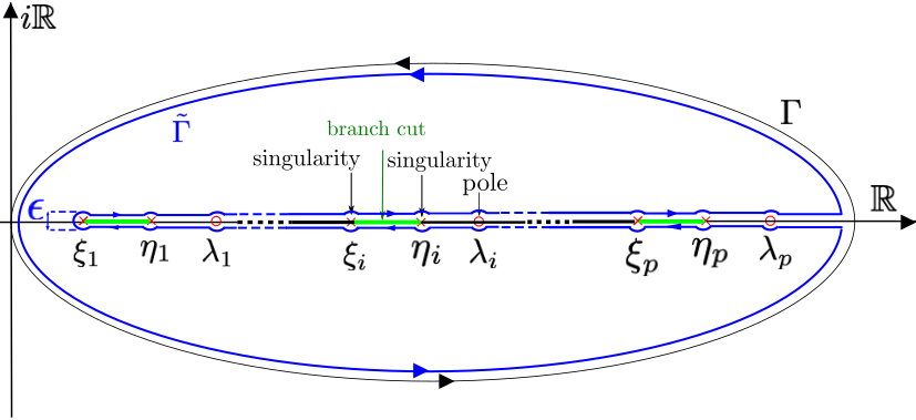
Figure 1: Deformation of the initial contour $\Gamma$ (in black) into the new contour $\tilde{\Gamma}$ (in blue). The branch cuts are represented in green (i.e., real $z$’s for which the argument of $\varphi(z)\psi(z)$ is negative).

Evaluating the estimate from Theorem 1 for $f(z)=\sqrt{z}$ then requires to evaluate a complex integral involving rational functions and square roots of rational functions. Since the complex square root is multivalued, a careful control of “branch-cuts” is required. To perform this calculus, we deform the integration contour $\Gamma$ of Theorem 1 into $\tilde{\Gamma}$ as per Figure 1. In the case $n_{1}\neq n_{2}$, the closed null-integral contour $\tilde{\Gamma}$ (blue in Figure 1) is the sum of the sought-for integral over $\Gamma$ and of four extra components:

1. Integrals over $\epsilon$-radius circles around $\xi_{i}$: those are null in the limit $\epsilon\to 0$, as confirmed by a change of variable $z=\xi_{i}+\epsilon e^{\imath\theta}$ which allows one to bound the integrand;

2. Integrals over the real axis (in the $\epsilon\to 0$ limit):

   $$A_{2}=\frac{n_{2}}{\pi p}\sum_{j=1}^{p}\int_{\xi_{j}+\epsilon}^{\eta_{j}-\epsilon}\sqrt{-(\varphi_{p}\psi_{p})(x)}\left[2\frac{\psi_{p}^{{}^{\prime}}(z)}{\psi_{p}(z)}\right.$$

   $$-\left.\left(\frac{\varphi_{p}^{{}^{\prime}}(z)}{\varphi_{p}(z)}+\frac{\psi_{p}^{{}^{\prime}}(z)}{\psi_{p}(z)}\right)\right]dx$$

   $$=\frac{2n_{2}}{\pi p}\sum_{j=1}^{p}\int_{\xi_{j}}^{\eta_{j}}\sqrt{-\varphi_{p}\psi_{p}(x)}\left[\frac{\psi_{p}^{{}^{\prime}}(z)}{\psi_{p}(z)}\right]dx$$

   $$-\frac{n_{2}}{\pi p}\sum_{j=1}^{p}\int_{\xi_{j}+\epsilon}^{\eta_{j}-\epsilon}\frac{\sqrt{-\varphi_{p}\psi_{p}(x)}}{\varphi_{p}\psi_{p}(x)}\left[\frac{d}{dx}\left(\varphi_{p}(x)\psi_{p}(x)\right)\right]dx$$

   $$=\frac{2n_{2}}{\pi p}\!\sum_{j=1}^{p}\int_{\xi_{j}}^{\eta_{j}}\!\sqrt{-\frac{\varphi_{p}(x)}{\psi_{p}(x)}}\psi_{p}^{\prime}(x)dx$$

   $$-2\frac{n_{2}}{\pi p}\sum_{j=1}^{p}\frac{1}{\sqrt{\epsilon\frac{d}{dx}\left(\frac{1}{(\varphi_{p}\psi_{p}(x))}\right)(\eta_{j})}}+o(\epsilon)$$

3. Integrals over the $\epsilon$-radius circles around $\eta_{j}$, with $\epsilon\to 0$

   $$A_{3}=2\frac{n_{2}}{\pi p}\sum_{j=1}^{p}\frac{1}{\sqrt{\epsilon\frac{d}{dx}\left(\frac{1}{(\varphi_{p}\psi_{p}(x))}\right)(\eta_{j})}}+o(\epsilon)$$

   which thus compensates the last ($\epsilon$-diverging) term in $A_{2}$.

4. Residues in the $\lambda_{j}$ poles

   $$A_{4} =2\frac{n_{2}}{p}\lim_{z\to\lambda_{j}}\sum_{j=1}^{p}\sqrt{(\varphi_{p}\psi_{p})(z)}=2\frac{n_{2}}{p}\sqrt{\frac{n_{1}}{n_{2}}}\sum_{j=1}^{p}\sqrt{\lambda_{j}}.$$

Putting these terms together entails the result of the theorem for the case where $n_{1}\neq n_{2}$. For $n_{1}=n_{2}$, it suffices to take the limit of the expression as $\xi_{j}\to\eta_{j}$. This yields:

$$\hat{D}(X_{1},X_{2};\sqrt{\cdot}) =\frac{2n_{1}}{p}\sum_{j=1}^{p}\sqrt{\lambda_{j}}$$

$$+\frac{2n_{1}}{p}\!\sum_{j=1}^{p}\frac{1}{\pi}\lim_{t\rightarrow\xi_{j}}\int_{\xi_{j}}^{t}\!\sqrt{-\frac{\varphi_{p}(x)}{\psi_{p}(x)}}\psi_{p}^{\prime}(x)dx$$

$$=\frac{2n_{1}}{p}\sum_{j=1}^{p}\sqrt{\lambda_{j}}$$

$$-\frac{2n_{1}}{p}\!\sum_{j=1}^{p}\frac{1}{2\pi\imath}\lim_{\epsilon\rightarrow 0}\oint_{\Gamma_{\xi_{j}}^{\epsilon}}\!\sqrt{-\varphi_{p}\psi_{p}(x)}\frac{\psi_{p}^{\prime}(x)}{\psi_{p}(x)}dx$$

where $\Gamma_{\xi_{j}}^{\epsilon}$ is an $\epsilon$-radius circular contour around $\xi_{j}$. The second equality is obtained by deforming the real integral in the complex plane (see [13] for complex analysis details). The result unfolds by letting ${z=\xi_{i}+\epsilon e^{\imath\theta}}$.

∎

Consequently, we obtain the following $n,p$-consistent estimate for the Wasserstein distance $D_{W}(C_{1},C_{2})$ of (1).

Corollary 1 (Consistent Estimate of $D_{W}(C_{1},C_{2})$).

Under Assumption 1,

$$\frac{1}{p}D_{W}(C_{1},C_{2})-\left[\frac{1}{p}{\rm tr}(\hat{C}_{1}+\hat{C}_{2})-2\hat{D}(X_{1},X_{2};\sqrt{\cdot})\right]\overset{\rm a.s.}{\longrightarrow}0$$ (7)

for $\hat{D}(X_{1},X_{2};\sqrt{\cdot})$ given by Theorem 2.

Remark 1 (Estimation of $\|C_{1}-C_{2}\|_{F}^{2}$).

The Frobenius distance between two covariance matrices also falls under the scope of the present article for the function $f(z)=z$. Indeed,

$$D_{F}(C_{1},C_{2}) =\|C_{1}-C_{2}\|_{F}^{2}={\rm tr}\left(C_{1}^{2}+C_{2}^{2}\right)-2{\rm tr}\left(C_{1}C_{2}\right).$$

Then under Assumption 1 and along with the fact that $\frac{1}{p}{\rm tr}C_{1}^{2}$ can be estimated consistently from $\frac{1}{p}{\rm tr}\hat{C}_{1}^{2}-\frac{1}{n_{1}p}({\rm tr}\hat{C}_{1})^{2}$,

$$\frac{1}{p}D_{F}(C_{1},C_{2})- \left[\frac{1}{p}{\rm tr}(\hat{C}_{1}^{2}+\hat{C}_{2}^{2})-\frac{p}{n_{1}}\left(\frac{1}{p}{\rm tr}\hat{C}_{1}\right)^{2}\right.$$

$$\left.-\frac{p}{n_{2}}\left(\frac{1}{p}{\rm tr}\hat{C}_{2}\right)^{2}-2\hat{D}(X_{1},X_{2};\cdot)\right]\overset{\rm a.s.}{\longrightarrow}0.$$

In this case, $\hat{D}(X_{1},X_{2};\cdot)$ assumes the simple expression

$$\hat{D}(X_{1},X_{2};\cdot) =\frac{1}{p}\sum_{j=1}^{p}\lambda_{j}=\frac{1}{p}{\rm tr}\hat{C}_{1}\hat{C}_{2}$$

which follows from $\frac{1}{p}{\rm tr}\hat{C}_{1}\hat{C}_{2}-\frac{1}{p}{\rm tr}C_{1}C_{2}\overset{\rm a.s.}{\longrightarrow}0$ (by elementary probability arguments) or equivalently from a residue calculus based on Theorem 1 for $f(z)=z$.

IV Simulations and Applications

In this section, we first corroborate our theoretical findings by comparing the classical plug-in estimator to our proposed estimator on synthetic Gaussian data. We then provide an application of our results to improved covariance matrix estimation based on few samples.

IV-A Confirmation of our results on synthetic data

We here compare the classical plug-in estimate of the Wasserstein distance (that is (1) with $C_{a}$ replaced by $\hat{C}_{a}$, $a=1,2$) with our proposed estimate in Corollary 1. Table I lists the results obtained for Toeplitz matrices $C_{1},C_{2}$ estimated based on various values of $p,n_{1},n_{2}$. While our proposed estimator is designed under a large $p,n_{1},n_{2}$ assumption (as per Assumption 1), it achieves competitive performances even for small values of $p$, corroborating here our findings in [8] for other classes of covariance matrix distances.

$p$	$D_{\rm W}(C_{1},C_{2})$	Classical	Proposed
2	0.0110	0.0127	0.0120
4	0.0175	0.0198	0.0183
8	0.0208	0.0232	0.0206
16	0.0225	0.0280	0.0227
32	0.0233	0.0339	0.0234
64	0.0237	0.0451	0.0240
128	0.0239	0.0667	0.0244
256	0.0240	0.1092	0.0244
512	0.0241	0.1953	0.0245

(error $<$ 5%) (error $>$ 50%) (error $>$ 100%) (error $>$ 300%)

TABLE I: Estimators of the Wasserstein distance between $C_{1}$ and $C_{2}$ with $[C_{1}]_{ij}=.2^{|i-j|}$, $[C_{2}]_{ij}=.4^{|i-j|}$, $x_{i}^{(a)}\sim\mathcal{N}(0,C_{a})$; $n_{1}=1024$ and $n_{2}=2048$ for different $p$. Averaged over $100$ trials.

IV-B Application to covariance matrix estimation

As a concrete application, Theorem 1 may be used to improve the actual estimation of covariance matrices under a small number $n\sim p$ of sample data, as similarly performed in [14] for other covariance matrix distances.

The idea is as follows: we first particularize Theorem 1 and Theorem 2 to the case where one of the covariance matrices, say $C_{1}$, is known by taking $c_{1}=0$ (i.e., $n_{1}\to\infty$ for all fixed $p$). This gives access to estimates for $D_{W}(M,C_{2};\sqrt{\cdot})$ for all deterministic positive definite matrix $M$. We then minimize this estimated distance over $M$ in order to estimate $C_{2}$ by means of a gradient descent approach.

For $C_{1}$ known, we redefine ${\mu_{p}=\frac{1}{p}\sum_{i=1}^{p}\delta_{\lambda_{i}(C_{1}\hat{C}_{2})}}$ and obtain, as a corollary of Theorem 1:

Theorem 3.

Let $\Gamma\subset\{z\in\mathbb{C},{\rm real}[z]>0\}$ a contour surrounding $\cup_{p=1}^{\infty}{\rm supp}(\mu_{p})$. Then,

$$D(C_{1},C_{2};f)-\frac{1}{2\pi ic_{2}}\oint_{\Gamma}F\left(-m_{\tilde{\mu}_{p}}(z)\right)dz\overset{\rm a.s.}{\longrightarrow}0$$

with $m_{\tilde{\mu}_{p}}(z)=\frac{p}{n_{2}}m_{{\mu}_{p}}(z)+\frac{p-n_{2}}{n_{2}z}$ and $F^{\prime}(z)=f(\frac{1}{z})$.

Proof.

For $C_{1}$ known ($c_{1}\to 0$), $\varphi_{p}(z)=z$, and the estimator of Theorem 1 yields:

$$\hat{D}(X_{1},X_{2};f)=\frac{1}{2\pi i}\oint_{\Gamma}\!f\left(\frac{z}{\psi_{p}(z)}\right)\left[\frac{\psi_{p}^{\prime}(z)}{\psi_{p}(z)}-\frac{1}{z}\right]\frac{\psi_{p}(z)dz}{c_{2}}.$$

Using the relation $m_{\tilde{\mu}_{p}}(z)=-\frac{\psi_{p}(z)}{z}$, we then get

$$\hat{D}(X_{1},X_{2};f)=-\frac{1}{2\pi ic_{2}}\oint_{\Gamma}\!f\left(-\frac{1}{m_{\tilde{\mu}_{p}}(z)}\right)m_{\tilde{\mu}_{p}}^{\prime}(z)zdz$$

and the result is immediate after an integration by parts. ∎

For $f(z)=\sqrt{z}$, one has $F(z)=2\sqrt{z}$ and we obtain, with a similar proof as for Theorem 2,

$$D(C_{1},C_{2};\sqrt{\cdot})-\hat{D}(C_{1},X_{2};\sqrt{\cdot})\overset{\rm a.s.}{\longrightarrow}0,$$

$$\hat{D}(C_{1},X_{2};\sqrt{\cdot})=\frac{2}{\pi c_{2}}\sum_{j=1}^{p}\int_{\xi_{j}}^{\lambda_{j}}\sqrt{m_{\tilde{\mu}_{p}(x)}}dx.$$

Our objective is now to exploit the fact that

$$C_{2}=\operatorname{argmin}_{M\succ 0}D_{W}(M,C_{2})$$ (8)

where the minimization is over the open cone of positive definite matrices. Using the approximation $D(M,C_{2};\sqrt{\cdot})\simeq\hat{D}(M,X_{2};\sqrt{\cdot})$, we are then tempted to minimize $\frac{1}{p}{\rm tr}(M+\hat{C}_{2})-2\hat{D}(M,X_{2};\sqrt{\cdot})$ in place of $D_{W}(M,C_{2})$. The former quantity however has a non zero probability to be negative, and we thus instead propose to estimate $C_{2}$ as:

$$\check{C}_{2} =\operatorname{argmin}_{M}h(M)$$

$$\quad h(M) =\left[\frac{1}{p}{\rm tr}(M+\hat{C}_{2})-2\hat{D}(M,X_{2};\sqrt{\cdot})\right]^{2}.$$

To compute the gradient $\nabla h(M)$ of $h$ at position $M$, one needs to evaluate the differential ${\rm D}h(M)[\xi]$, at $M$ and in the direction $\xi$, in the Riemmanian manifold of $p\times p$ symmetric positive definite matrices (see [15, 14] to further technical details). We then use the relation ${\rm D}h(M)[\xi]=\langle\nabla h(M),\xi\rangle_{M}$ where $\langle\cdot,\cdot\rangle_{.}$ is the Riemmanian metric defined as $\langle\eta,\xi\rangle_{M}={\rm tr}\left(M^{-1}\eta M^{-1}\xi\right)$. We obtain the relation

$$\pi\imath p\frac{\nabla h(M)}{2\sqrt{h(M)}}=\frac{1}{p}M^{2}$$

$$+\sum_{j=1}^{p}\int_{\xi_{j}}^{\lambda_{j}}\sqrt{\frac{1}{m_{\tilde{\mu}_{p}}(x)}}{\rm sym}\left(M\hat{C}_{2}(M\hat{C}_{2}-xI_{p})^{-2}M\right)dx$$

where ${\rm sym}(A)=\frac{1}{2}(A+A^{\sf T})$ is the symmetric part of $A\in\mathbb{R}^{p\times p}$. We can write the latter as:

$$\nabla h(M)=2\sqrt{h(M)}\left[{\rm sym}\left(V\Lambda_{\nabla}V^{-1}\right)+\frac{1}{p}M^{2}\right]$$

where $V$ is the orthogonal matrix of the eigenvectors of $M\hat{C}_{2}$ and $\Lambda_{\nabla}$ is the diagonal matrix with

$$\left[\Lambda_{\nabla}\right]_{kk} =\frac{1}{\pi p}\sum_{j\neq k}\int_{\xi_{j}}^{\lambda_{j}}\sqrt{\frac{1}{m_{\tilde{\mu}_{p}}(x)}}\frac{1}{(\lambda_{k}-x)^{2}}dx$$

$$+\frac{1}{\pi p}\sum_{j\neq k}\int_{\xi_{k}}^{\lambda_{k}}\sqrt{\frac{1}{m_{\tilde{\mu}_{p}}(x)}}\frac{1}{(\lambda_{j}-x)^{2}}dx.$$

This finally entails the gradient descent Algorithm 1.

Require Positive definite initialization $M=M_{0}$.

Repeat $M\leftarrow M^{\frac{1}{2}}\exp\left(-tM^{-\frac{1}{2}}\nabla h(M)M^{-\frac{1}{2}}\right)M^{\frac{1}{2}}$ with $t$ either fixed or optimized by backtracking line search.

Until Convergence.

Return $M$.

Algorithm 1 Proposed estimation algorithm.

Figure 2 depicts the results of the algorithm. There is displayed the Wasserstein distance $D_{W}(C,\cdot)$ between a matrix $C$ having four distinct eigenvalues of equal multiplicity (precisely, $\nu_{p}=\frac{1}{4}(\delta_{.1}+\delta_{3}+\delta_{4}+\delta_{5})$) and various estimators of $C$: the sample covariance matrix (SCM), the state-of-the-art “non-linear shrinkage” estimators QuEST1 [16] (based on a Frobenius distance minimization) and QuEST2 [17] (based on a Stein loss minimization), and the result of the gradient descent approach proposed in this section. For fair comparison, the iterative QuEST1, QuEST2 and our proposed method are all initialized at $M_{0}$ the linear shrinkage estimator from [18]. Note that our proposed choice of $C$ is particularly suited to mimick an “optimal transport” problem of displacing the eigenvalues of $M_{0}$ to the discrete four positions of the eigenvalues of $C$.

In addition to the computational simplicity of our gradient-descent approach with respect to the QuEST estimators (see the numerical method details in [19]), the figure demonstrates significant gains brought by our proposed approach for large values of $p/n$, where the SCM particularly fails.

V Concluding Remarks

Interestingly, while the Fisher distance or Kullbach-Liebler divergence, which depend on logarithms of inverse of covariance matrices, are understandably difficult to estimate in the $n_{1},n_{2}<p$ regime (see [10] for advanced discussions on this matter), the Wasserstein distance should not be confronted with this limitation. Yet, the invertibility of $C_{1},C_{2}$ and the request for $c_{1},c_{2}\in(0,1)$ (i.e., $p<n_{1},n_{2}$) from Assumption 1 are fundamental to our proofs. Precisely, the variable changes exploited in the proof of Theorem 1 to reach a contour $\Gamma_{\nu}$ correctly surrounding ${\rm supp}(\nu_{p})$ from a contour $\Gamma$ surrounding ${\rm supp}(\mu_{p})$ are not satisfying if $c_{1}>1$ or $c_{2}>1$. These surprising difficulties need clarification.

Another point of interest lies in the comparative advantage of exploiting a particular covariance matrix distance in specific scenarios. For instance, it may seem that ill-conditioned matrices should be more tolerated by Wasserstein distance estimators than by Fisher distance estimators. Yet, this aspect is not obvious in our proofs and also deserves more insights.

References

- [1] Gaspard Monge, “Mémoire sur la théorie des déblais et des remblais,” Histoire de l’Académie Royale des Sciences de Paris, 1781.
- [2] Leonid V Kantorovich, “On the translocation of masses,” in Dokl. Akad. Nauk. USSR (NS), 1942, vol. 37, pp. 199–201.
- [3] Yossi Rubner, Carlo Tomasi, and Leonidas J Guibas, “The earth mover’s distance as a metric for image retrieval,” International journal of computer vision, vol. 40, no. 2, pp. 99–121, 2000.
- [4] Zhengyu Su, Yalin Wang, Rui Shi, Wei Zeng, Jian Sun, Feng Luo, and Xianfeng Gu, “Optimal mass transport for shape matching and comparison,” IEEE transactions on pattern analysis and machine intelligence, vol. 37, no. 11, pp. 2246–2259, 2015.
- [5] Kangyu Ni, Xavier Bresson, Tony Chan, and Selim Esedoglu, “Local histogram based segmentation using the wasserstein distance,” International journal of computer vision, vol. 84, no. 1, pp. 97–111, 2009.
- [6] Marco Cuturi, “Sinkhorn distances: Lightspeed computation of optimal transport,” in Advances in neural information processing systems, 2013, pp. 2292–2300.
- [7] X. Mestre, “On the asymptotic behavior of the sample estimates of eigenvalues and eigenvectors of covariance matrices,” vol. 56, no. 11, pp. 5353–5368, Nov. 2008.
- [8] Romain Couillet, Malik Tiomoko, Steeve Zozor, and Eric Moisan, “Random matrix-improved estimation of covariance matrix distances,” arXiv preprint arXiv:1810.04534, 2018.
- [9] Gabriel Peyré and Marco Cuturi, “Computational optimal transport,” Foundations and Trends® in Machine Learning, vol. 11, no. 5-6, pp. 355–607, 2019.
- [10] Romain Couillet, Malik Tiomoko, Steeve Zozor, and Eric Moisan, “Random matrix-improved estimation of covariance matrix distances,” arXiv preprint arXiv:1810.04534, 2018.
- [11] J. W. Silverstein and Z. D. Bai, “On the empirical distribution of eigenvalues of a class of large dimensional random matrices,” Journal of Multivariate Analysis, vol. 54, no. 2, pp. 175–192, 1995.
- [12] Joel N Franklin, Matrix theory, Courier Corporation, 2012.
- [13] EB Saff and AD Snider, “Fundamentals of complex analysis with applications to engineering and science,” 2003.
- [14] Malik Tiomoko, Florent Bouchard, Guillaume Ginholac, and Romain Couillet, “Random matrix improved covariance estimation for a large class of metrics,” arXiv preprint arXiv:1902.02554, 2019.
- [15] P-A Absil, Robert Mahony, and Rodolphe Sepulchre, Optimization algorithms on matrix manifolds, Princeton University Press, 2009.
- [16] Olivier Ledoit and Michael Wolf, “Spectrum estimation: A unified framework for covariance matrix estimation and pca in large dimensions,” Journal of Multivariate Analysis, vol. 139, pp. 360–384, 2015.
- [17] Olivier Ledoit, Michael Wolf, et al., “Optimal estimation of a large-dimensional covariance matrix under stein’s loss,” Bernoulli, vol. 24, no. 4B, pp. 3791–3832, 2018.
- [18] Olivier Ledoit and Michael Wolf, “A well-conditioned estimator for large-dimensional covariance matrices,” Journal of multivariate analysis, vol. 88, no. 2, pp. 365–411, 2004.
- [19] Olivier Ledoit and Michael Wolf, “Numerical implementation of the quest function,” Computational Statistics & Data Analysis, vol. 115, pp. 199–223, 2017.