Efficient Selection of Quasar Candidates Based on Optical and Infrared Photometric Data Using Machine Learning

Abstract

We aim to select quasar candidates based on the two large survey databases, Pan-STARRS and AllWISE. Exploring the distribution of quasars and stars in the color spaces, we find that the combination of infrared and optical photometry is more conducive to select quasar candidates. Two new color criterions (yW1W2 and iW1zW2) are constructed to distinguish quasars from stars efficiently. With izW1W2, 98.30% of star contamination is eliminated, while 99.50% of quasars are retained, at least to the magnitude limit of our training set of stars. Based on the optical and infrared color features, we put forward an efficient schema to select quasar candidates and high redshift quasar candidates, in which two machine learning algorithms (XGBoost and SVM) are implemented. The XGBoost and SVM classifiers have proven to be very effective with accuracy of $99.46\%$ when 8Color as input pattern and default model parameters. Applying the two optimal classifiers to the unknown Pan-STARRS and AllWISE cross-matched data set, a total of 2,006,632 intersected sources are predicted to be quasar candidates given quasar probability larger than 0.5 (i.e. $P_{\mathrm{QSO}}>0.5$). Among them, 1,201,211 have high probability ($P_{\mathrm{QSO}}>0.95$). For these newly predicted quasar candidates, a regressor is constructed to estimate their redshifts. Finally 7,402 $z>3.5$ quasars are obtained. Given the magnitude limitation and site of the LAMOST telescope, part of these candidates will be used as the input catalogue of the LAMOST telescope for follow-up observation, and the rest may be observed by other telescopes.

1 Introduction

Quasars are high-luminosity objects that are observed at extremely distant distances, up to 12.9 billion light-years (Mortlock et al., 2011), and they are believed to be powered by the accretion onto supermassive black holes (SMBHs) in the centers of galaxies (Antonucci, 1993). By tracing the properties of quasars, we may understand supermassive black holes in massive galaxies, and the coevolution of black holes and their host galaxies (Kormendy & Ho, 2013). So far, quasars have been found to distribute on a very wide redshift range from 0 to over 7 (Mortlock et al., 2011). High redshift quasars can be taken as important probes for the formation and evolution of structure in the early universe (Fan, 2006).

Since the first quasar was discovered in 1963 (Schmidt, 1963), the number of quasars has grown significantly, especially after the implementation of many wide-field spectroscopical surveys, such as the Two-Degree Field Quasar Redshift Survey (2dF; Croom et al. 2004), the Sloan Digital Sky Survey (SDSS; York et al. 2000) and Large Sky Area Multi-Object Fiber Spectroscopic Telescope (LAMOST; Cui et al. 2012).

SDSS has conducted several quasar surveys in its different phases. The quasar program of SDSS-I/II led to the discovery of redshift z > 5 quasars (Fan et al., 1999) and provided the DR7 quasar catalog (DR7Q; Schneider et al. 2010), which contains more than 105,000 quasars. The SDSS-III Baryon Oscillation Spectroscopic Survey (BOSS; Ross et al. 2012; Dawson et al. 2013) has discovered about 270,000 quasars, mostly in the redshift range $2.15-3.5$, which were released in DR12 quasar catalog (DR12Q; Pâris et al. 2017). SDSS-IV extended Baryon Oscillation Spectroscopic Survey (eBOSS; Myers et al. 2015; Dawson et al. 2016) concentrates its efforts on the observation of galaxies and in particular quasars. The SDSS-DR14 quasar catalog (DR14Q, Pâris et al. 2018), which is the first to be released that contains new identifications from eBOSS, contains 526,356 quasars among which 144,046 are new discoveries.

So many quasars have been discovered mainly depending on large photometric sky survey projects (for example, GALEX, SDSS, Pan-STARRS, WISE, 2MASS) and efficient selection of quasar candidates. There are various approaches focusing on targeting quasar candidates, which groups into color-color cut, variability selection and machine learning algorithms. The color-color cut methods consist of ultraviolet (UV)-excess (e.g. Richards et al. 2009), the KX-technique (e.g. Nakos et al. 2009; Maddox et al. 2012), color selection of UV and optical data (e.g. Worseck & Prochaska 2011), color-color diagram based on optical and infrared data (e.g. Wu & Jia 2010; Wang et al. 2016). As for variability selection, MacLeod et al. (2011) and Butler & Bloom (2011) selected quasar candidates based on photometric variability by a damped random walk model; Palanque-Delabrouille et al. (2016a) presented the variability selection of quasars in eBOSS; Graham et al. (2014) introduced Slepian wavelet variance (SWV) for quasar selection.

With the increase of astronomical data, machine learning algorithms are popular and widely applied on quasar candidate selection, for example, the probabilistic principal surfaces and the negative entropy clustering (D’Abrusco et al., 2009), Bayesian selection method (e.g., Richards et al. 2004; Kirkpatrick et al. 2011; Peters et al. 2015), artificial neural networks (ANNs; e.g. Yèche et al. 2010; Tuccillo et al. 2015), extreme deconvolution (e.g. Bovy et al. 2011; Ross et al. 2012; Myers et al. 2015), support vector machine (SVM; e.g. Gao et al. 2008; Peng et al. 2012), random forest algorithm (e.g. Schindler et al. 2017). Other techniques based on radio, X-ray bands are also developed. McGreer et al. (2009) obtained quasar candidates using radio criteria from SDSS database; Khorunzhev et al. (2016) selected quasar candidates among X-Ray sources from the 3XMM-DR4 survey of the XMM-Newton observatory.

Besides SDSS, Pan-STARRS is another important optical sky survey project. Therefore it is of great value for increasing the number of quasar candidates from Pan-STARRS. Based on Pan-STARRS and WISE data, we aim at the efficient selection of quasar candidates in this paper. The photometric data used for our candidate selection as well as known quasars and stars are presented, and the rejection of extended objects is discussed (Section 2). Section 3 describes the color-color cut to perform the selection of quasar candidates based on near-IR/infrared photometry. The principles of support vector machine (SVM) and XGBoost are introduced in Section 4. Machine-learning algorithms are further explored to classify quasar candidates and their performances are compared. In Section 5, an XGBoost regressor is constructed to estimate quasar redshifts and applied to our newly predicted quasar candidates. At last, a quasar candidate catalogue with the estimated redshifts is obtained as well as another catalogue that meets the observed conditions of the LAMOST telescope. The experimental results and their applications are finally summarized in Section 6.

2 The Data

2.1 PS1 Photometry

Pan-STARRS is a wide-field optical/near-IR survey telescope system located at the Haleakala Observatory on the island of Maui in Hawaii. Similar to SDSS, it provides five band photometries ($g_{\mathrm{P1}},r_{\mathrm{P1}},i_{\mathrm{P1}},z_{\mathrm{P1}},y_{\mathrm{P1}}$). The PS1 survey (Chambers et al., 2016) is the first part of Pan-STARRS to be completed. The 3$\pi$ survey is the largest survey PS1 has performed, covering the entire north to $-30$ deg declination. The 5$\sigma$ median limiting AB magnitudes in the five PS1 bands $grizy$ are 23.2, 23.0, 22.7, 22.1 and 21.1 mag, respectively. The Pan-STARRS photometry is extinction-corrected by the extinction coefficients $\alpha_{g}$, $\alpha_{r}$, $\alpha_{i}$, $\alpha_{z}$, $\alpha_{y}$ = 3.172, 2.271, 1.682, 1.322, 1.087 with the extinction values from the SDSS photometry (Schlafly & Finkbeiner, 2011). We set MagErr $<$ 0.2 for $g_{\mathrm{P1}},r_{\mathrm{P1}},i_{\mathrm{P1}},z_{\mathrm{P1}},y_{\mathrm{P1}}$ bands to exclude sources with large uncertainty, and set psf_qf_perfect $>$ 0.95 to remove observations which land on bad parts of the detector according to the work (Hernitschek et al., 2016).

2.2 WISE Photometry

WISE (Wright et al., 2010) is an infrared-wavelength astronomical space telescope launched by NASA and has mapped the entire sky at 3.4, 4.6, 12 and 22 $\mu m$ ($W1$, $W2$, $W3$, $W4$). The 5$\sigma$ limiting AB magnitudes of the AllWISE catalog in $W1$, $W2$, $W3$ and $W4$ bands are 19.6, 19.3, 16.7, and 14.6 mag, separately. The angular resolutions in each band are 6.1, 6.4, 6.5 and 12 arcsec, respectively. We only use photometric data in $W1$ and $W2$ bands, because $W3$ and $W4$ are much shallower and have larger magnitude errors.

To remove poor quality sources, some restrictions are set on primary detection and information flags. Unknown sources that meet the following conditions will be removed:

(i) Sources with high magnitude error and low signal-to-noise ratio ($\sigma_{\mathrm{W}1}>0.3$, $\sigma_{\mathrm{W}2}>0.3$, $SNR_{\mathrm{W}1}<3$, $SNR_{\mathrm{W}2}<3$).

(ii) Sources sources that are marked as saturated in the detection ($\mathtt{W1sat}\neq 0$, $\mathtt{W2sat}\neq 0$).

(iii) Objects affected by diffraction spikes, ghosts, latent images, and scattered light in both $W1$ and $W2$ ($\mathtt{cc\_flags}\neq 0$).

(iv) Marked as extended sources in WISE detection ($\mathtt{ext\_flg}\neq 0$).

(v) Small-separation and same-Tile (SSST) detection ($\mathtt{rel}\neq 0$).

(vi) Affected by the nearby sources in the process of profile-fitting ($\mathtt{nb}>1$).

We cross match the Pan-STARRS1 MeanObject table with AllWISE to obtain the source containing optical and infrared photometric information. The match radius is set to 3 arcsec.

2.3 Spectroscopically Identified Quasar and Star samples

We use the latest SDSS Data Release 14 Quasar Catalog (DR14Q; Pâris et al. 2018) as the known quasar sample. It contains 526,356 spectroscopically identified quasars, among which 144,046 are new discoveries from the latest SDSS-IV eBOSS survey (Myers et al., 2015; Dawson et al., 2016). DR14Q also includes previous spectroscopically identified quasars from SDSS-I, II and III.

Spectroscopically identified stellar sample is acquired from the SpecPhotoAll table in SDSS DR14 using CASJOB. Similar to Peng et al. (2012), the sample meets the limitation of class $=$ STAR, sciencePrimary $=$ 1, Mode $=$ 1 and zWarrning $=$ 0. The records with fatal errors are rejected using flags such as BRIGHT, SATURATED, EDGE and BLENDED. Finally, a catalogue of 747,852 spectroscopically identified stars is obtained through the query.

In this article, we focus on Pan-STARRS and AllWISE datasets, so we match the SDSS known quasar and star samples with Pan-STARRS and AllWISE to obtain PS1 and AllWISE photometry. The match radius is set to 3 arcsec. After matching and adding photometric quality limits (See $\S$2.1 and $\S$2.2) to remove poor quality sources, we obtain our known samples with Pan-STARRS and WISE photometry. After that, the number of stars is 355,255, that of quasars is 261,735. Table 1 details the star sample that has all values of PS1 photometry and W1W2 photometry for each subclass. The top panel of Figure 1 shows the $r$ magnitude distribution of quasars and stars. It can be seen that stars are much brighter than quasars in our known samples. The median $r$ magnitude of stars is 17.2 while that of quasars is 19.8. The bottom panel of Figure 1 shows the redshift distribution of known quasars.

Table 1: Spectroscopic Classes of Known Stars.

Spectral Class	No. of objects
O	105
OB	21
B	302
A	19,340
F	143,882
G	27,538
K	85,001
M	76,734
L	148
T	49
WD	848
CV	716
Carbon	571
Total No.	355,255

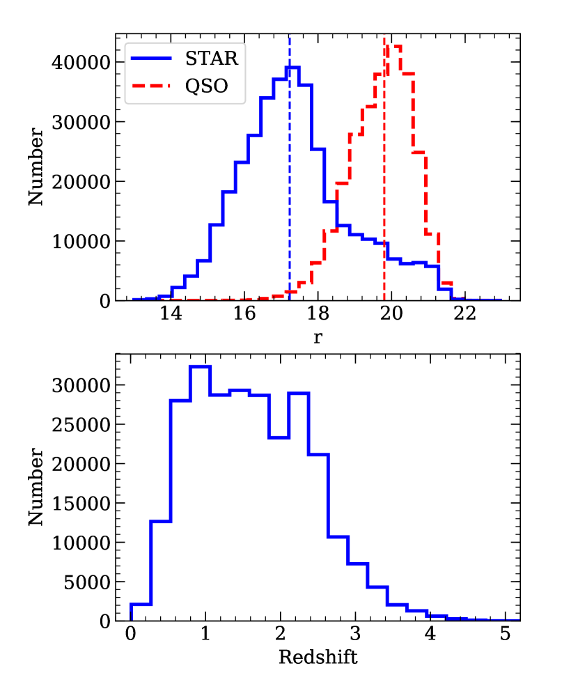
Figure 1: The top panel shows the $r$ magnitude distribution of known quasars and stars that have all photometries of $g_{\mathrm{P}1},r_{\mathrm{P}1},i_{\mathrm{P}1},z_{\mathrm{P}1},y_{\mathrm{P}1},W1,W2$. The vertical dashed lines represent the median magnitude values of stars and quasars, respectively. The bottom panel shows the redshift distribution of known quasars that have all photometries of $g_{\mathrm{P}1},r_{\mathrm{P}1},i_{\mathrm{P}1},z_{\mathrm{P}1},y_{\mathrm{P}1},W1,W2$.

3 Selection quasar candidates base on Optical and Infrared photometry

3.1 Discrimination of resolved and unresolved sources

We focus on how to separate quasars from stars, so galaxies should be excluded. We use PSFMag$-$KronMag cut on $i$ and $z$ bands to exclude galaxies. As shown in Figure 2, galaxies are clearly distinguished from stars and quasars in the distribution of iPSFMag$-$iKronMag and zPSFMag$-$zKronMag. The cut is set at iPSFMag$-$iKronMag $=$ 0.3 and zPSFMag$-$zKronMag $=$ 0.3 which is a strict limitation to exclude most galaxies. It can rule out $96.90\%$ of galaxies, with very few exceptions in our test on the known samples. But it should be noted that this strategy would not exclude optically compact, unresolved sources that are selected by WISE to have a low-level active black hole but that do not have a luminous black hole in the optical band. Some of these might be considered as low-luminosity AGN rather than genuine quasars. Some of them might also be Type-1 quasars rather than having broad lines (Zakamska et al., 2003; Reyes et al., 2008).

Applying this criterion to the unknown sample obtained by crossing Pan-STARRS1 and AllWISE, we obtain the pointed sources to be predicted in the following.

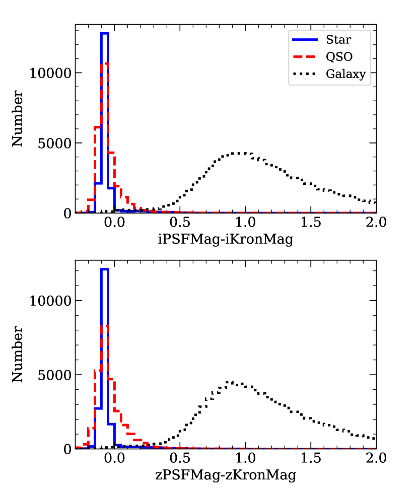
Figure 2: The distribution of iPSFMag$-$iKronMag and zPSFMag$-$zKronMag for known stars, quasars and galaxies.

3.2 The optical and infrared color cuts

We aim to find quasar candidates through more bands of photometric information from both optical and infrared bands. For this purpose, we describe known quasars and stars in the color-color space. In Figure 3 we give six color-color diagrams. The quasars are indicated in different colors according to their redshifts.

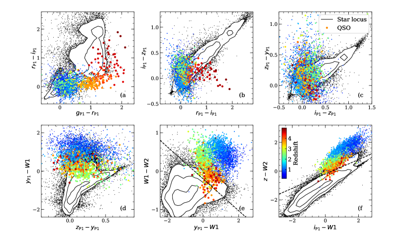
Figure 3: The distribution of known stars and quasars in the color spaces of Pan-STARRS1 and AllWISE photometry. The black outlines are the contours of star distribution and contain 68%, 94%, and 98.5% of the stars, respectively. Quasars are drawn in different colors and sizes according to their redshift values. In the panels (a)-(c), stars and quasars mostly overlap, in panel d, they overlap partly, while in panels (e)-(f) they are clearly separated. The new color cuts are displayed in dashed line.

It is easily found that quasars and stars are clearly separated in some color-color spaces (e.g. panels e-f), while more overlapping in other panels (e.g. panels a-d). It indicates that adding infrared photometry is very effective for selecting quasar candidates, as other authors have found (Stern et al., 2012; Assef et al., 2013), which overcomes the inefficiency of the pure optical selection. In the color space $y-W1$ vs. $W1-W2$ (panel e), quasars and stars occupy different regions, with few overlap. After examining known samples, we determine the cut that best separates the quasars and stars. In AB magnitude, the yW1W2 cut can be written as

$$W1-W2\geq-0.2-0.417\times(y_{\mathrm{P}1}-W1)\\$$ (1)

In the test, the above color criterion produces a very pure quasar sample from the mixture of stars and quasars. Of all 355,255 stars, 348,530($98.11\%$) of stars are ruled out, while 6,725 escape the color criterion. Of all 261,735 quasars, 260,095($99.37\%$) are included in the color criterion. However, by displaying quasars in different colors according to their redshift values, we find that higher redshift quasars are more likely to mix with stars.

In order to test the effect of this color criterion for selecting different redshift quasars, we divide the quasars into two parts: high redshift ($z>3.5$) and low redshift ($z\leq 3.5$). The result is that $11.38\%$ (424/3,724) high redshift quasars have been classified as stars while for low redshift quasars the ratio is only $0.47\%$ (1,216/258,011). Consistent with what Panel (e) indicates, this color criterion is more effective for selecting low redshift ($z\leq 3.5$) quasar candidates.

Another color-color space that is effective for distinguishing quasars from stars is the $i_{\mathrm{P}1}-W1$ vs. $z_{\mathrm{P}1}-W2$ color space (Panel (f)), in which quasars and stars are located in two different areas. After examining known samples, we obtain the iW1zW2 cut in AB magnitude that clearly discriminates quasars from stars.

$$z_{\mathrm{P}1}-W2\geq-0.2+0.5\times(i_{\mathrm{P}1}-W1)$$ (2)

This color criterion also greatly reduces the pollution of stars, with 349,217($98.30\%$) of stars removed, while keeping 260,427($99.50\%$) of quasars. For $z>3.5$ quasars, $9.43\%$ (351/3,724) are mixed into stars, while for $z\leq 3.5$ quasars, the value is $0.37\%$ (957/258,011).

In summary, the yW1W2 and iW1zW2 color cuts are very effective in selecting quasar candidates from the mixture of stars and quasars. Using these two color cuts, the majority of star contamination will be excluded, while the majority of quasars will be retained. However, one of the weaknesses of these two color cuts is that the high redshift quasars have a greater chance of being removed than the low redshift quasars. It seems difficult to completely exclude stars while retaining the vast majority of quasars only in a two-dimensional color-color space. So in this paper, we aim to use machine learning to select quasar candidates, in which stars and quasars can be better separated in higher dimensional color spaces.

4 Selection Quasar Candidates Base on Machine learning

4.1 Introduction to SVM

Support Vector Machines (SVM; Vapnik 1995) is a supervised machine learning algorithm used to solve classification and regression problems, especially for binary classification problems. The core idea of SVM is to find the best separation hyperplane in the feature space to separate the two classes. SVM maps the original feature vectors to a higher-dimensional space through the kernel function. Among all hyperplanes that can separate positive and negative samples, the best hyperplane is the one that has the largest margin between the data on both sides.

In binary classification, the training sample can be expressed as $T=\{\mn@boldsymbol{x}_{1},y_{1}\},...,\{\mn@boldsymbol{x}_{n},y_{n}\}$, where ${\mn@boldsymbol{x}}_{i}\in\mathtt{R}^{N}$, $y_{i}$ is the class label with the values $\{+1,-1\}$ for positive and negative classes, respectively. The separating hyperplane can be written as

$$\mn@boldsymbol{\omega}\cdot\mn@boldsymbol{x}_{i}+b=0\qquad i=1,2,.....n\\$$ (3)

We can get the optimal hyperplane with maximum margin by minimizing the following

$$F(\mn@boldsymbol{\omega},\mn@boldsymbol{\xi})=\frac{1}{2}(\mn@boldsymbol{\omega}\cdot\mn@boldsymbol{\omega})+C\sum_{i=1}^{n}\xi_{i}\\ \xi_{i}>0\\$$ (4)

subject to

$$y_{i}[(\mn@boldsymbol{\omega}\cdot\mn@boldsymbol{x}_{i}+b)]\geq 1-\xi_{i}\qquad i=1,2,.....n\\$$ (5)

Here $\xi$ is the slack variable which is introduced to allow the presence of points that are not completely separated by the hyperplane. The factor $C$ is the corresponding penalty coefficient for misclassification. The problem above can be solved by introducing the Lagrangian function, and it becomes the problem of solving the Lagrange multipliers $\alpha_{i}$ and $b$, as follows:

$$L(\omega,b,\alpha)=\sum_{i=1}^{n}\alpha_{i}-\frac{1}{2}\sum_{i,j=1}^{n}\alpha_{i}\alpha_{j}y_{i}y_{j}x_{j}x_{i}^{T}\\$$ (6)

subject to

$$\begin{split}&\alpha_{i}[1-y_{i}(\sum_{i=1}^{n}\alpha_{i}y_{i}\langle x_{j},x_{i}\rangle+b)]=0\\ &\sum_{i=1}^{n}\alpha_{i}y_{i}=0\\ &0\leq\alpha_{i}\leq C\\ \end{split}$$ (7)

SVM has been widely used in astronomy for star and galaxy classification (Zhang & Zhao, 2003, 2004; Bu et al., 2014; Liu et al., 2018; Sreejith et al., 2018), quasar candidate selection (Gao et al., 2008; Zhang et al., 2011; Kim et al., 2011; Peng et al., 2012) as well as quasar redshift estimation (Wang et al., 2008; Han et al., 2016).

4.2 Introduction to XGBoost

XGBoost (Chen & Guestrin, 2016) is a boosting algorithm that can be used for classification and regression problems. It was developed on the basis of Gradient Boosting Decision Tree (GBDT; Friedman 2001). Both XGBoost and GBDT are implementation of boosting method which aims to build strong classifiers by learning multiple weak classifiers. The biggest difference between XGBoost and GBDT is that GBDT only uses the first derivative of the loss function to calculate the residual, while XGBoost applies not only the first derivative but also the second derivative of the loss function. The predictors XGBoost builds are regression tree ensemble. For a given data set with $n$ examples and $m$ features $\texttt{D}=\{(x_{i},y_{i})\}(x_{i}\in\texttt{R},y_{i}\in\texttt{R})$. Set the model has $k$ trees totally. The prediction on $x_{i}$ is given by

$$\widehat{y_{i}}=\sum_{k=1}^{K}{f_{k}}(x_{i}),\quad{f_{k}}\in\texttt{F}$$ (8)

where $f_{k}$ is one regression tree, and $f_{k}(x_{i})$ is the score it gives to $x_{i}$. $\texttt{F}=\{f(x)=\omega_{q(x)}\}(q:\texttt{R}\rightarrow T,\omega\in\mathtt{R}^{\mathtt{T}})$ is the space of regression trees. Here $q(x)$ represents the structure function which is used to map each point to a leaf index. The learning of the set of functions used in the model is done by minimizing the following regularized objective:

$$Obj=\sum_{i}^{n}l(\widehat{y_{i}},y_{i})+\sum\Omega(f_{k})\\$$ (9)

where the first term $l$ is the loss function and the second term $\Omega$ penalizes the complexity of the model. We first discuss the first item. At the $t$-th iteration, it can be written as

$$Obj^{(t)} =\sum_{i}^{n}l(y_{i},\widehat{y_{i}}^{(t)})+\Omega(f_{t})$$ (10)

$$=\sum_{i}^{n}l(y_{i},\widehat{y_{i}}^{(t-1)}+f_{t}(x_{i}))+\Omega(f_{t})$$

The loss function can be written in the form of Taylor expansion and keep second-order accuracy.

$$Obj^{(t)}=\sum_{i=1}^{N}[g_{i}f_{t}(x_{i})+\frac{1}{2}h_{i}f_{t}^{2}(x_{i})]+\Omega(f_{t})$$ (11)

The $\Omega$ term is defined as complexity of the tree, it can be written as

$$\Omega(f_{t})=\gamma T+\frac{1}{2}\lambda\sum_{k=1}^{T}\omega_{k}^{2}$$ (12)

Here $T$ represents the number of leaves, $\omega_{j}$ represents the score given by the $j$-th leaf. Define $I_{j}=\{i|q(x_{i})=j\}$ as the instance set of leaf $j$. The objective is then expressed as

$$Obj^{(t)}=\sum_{j=1}^{T}[(\sum_{i\in I_{j}}g_{i})\omega_{j}+\frac{1}{2}(\lambda+\sum\limits_{i\in I_{j}}h_{i})\omega_{j}^{2}]+\gamma T$$ (13)

If the structure of a tree $q(x)$ is fixed, we can gain the optimal weight of leaf $j$ by setting the derivative of $\omega_{j}$ equal to zero. Setting $G_{i}=\sum_{i\in I_{j}}g_{i}$ and $H_{i}=\sum_{i\in I_{j}}h_{i}$, $\omega_{j}$ is changed as following

$$\omega_{j}^{*}=-\frac{G_{i}}{H_{i}+\lambda}$$ (14)

So $Obj^{(t)}$ can be simplified as

$$Obj^{(t)}(q)=-\frac{1}{2}\sum_{j=1}^{T}\frac{G_{i}^{2}}{H_{i}+\lambda}+\gamma T$$ (15)

In practice, an optimized greedy algorithm is always used to grow the tree. It starts from a single leaf and tries to add a best spilt for each existed leaf node, iteratively. After adding a spilt, the objective turns as follows:

$$\mathrm{Gain}=\frac{1}{2}[-\frac{(G_{L}+G_{R})^{2}}{H_{L}+H_{R}+\lambda}+\frac{(G_{L}^{2})}{H_{L}+\lambda}+\frac{G_{R}^{2}}{H_{R}+\lambda}]-\gamma$$ (16)

Gain is used to find the best spilt. For one possible spilt, XGBoost scans from left to right of the leaves to calculate the $G_{L}$ and $G_{R}$, $H_{L}$ and $H_{R}$, then the Gain can be calculated. Note that the formula has a penalty term $\gamma$ which can lead to a negative gain. A negative gain means that the newly added spilt does not make the algorithm perform better and should be cut off.

In astronomy, XGBoost was recently used for the separation of pulsar signals from noise (Bethapudi & Desai, 2018) and the classification of unknown source in the Fermi-LAT catalog (Mirabal et al., 2016).

4.3 Classification Metrics

There are many criterions to score the performance of a classifier. Here we only apply three standard metrics (Accuracy, Precision and Recall) to determine which one classifier is better. In binary classification, the accuracy is the ratio of the number of the correctly classified samples to the total number of the two classes of samples.

$$\mathrm{Accuracy}=\frac{TP+TN}{TP+TN+FP+FN}$$ (17)

Here TP is the positive sample that is correctly classified by the classifier. FP represents the negative sample that is classified as positive. FN refers to the positive sample that is classified as negative.

The precision (P) is the ratio of the true positive (negative) sample in all the samples that are predicted to be positive (negative). The Recall (R) is the ratio of correctly predicted positive (negative) samples in all the true positive (negative) samples.

$$\mathrm{Precison}=\frac{TP}{TP+FP},\mathrm{Recall}=\frac{TP}{TP+FN}$$ (18)

4.4 Binary Classifiers Construction of XGBoost and SVM

In this section, we detail how to use photometric information to construct XGBoost and SVM classifiers for quasar selection. The quasar and star training sets are introduced in §2.3. The input pattern used for SVM and XGBoost training is a combination of colors. To test the effect of different input patterns on the performance of a classifier, we build a classifier using different input patterns. The input feature is the colors, which is obtained from the magnitude difference between two different bands, like ($g_{\mathrm{P}1}-r_{\mathrm{P}1}$,$r_{\mathrm{P}1}-i_{\mathrm{P}1}$,$i_{\mathrm{P}1}-z_{\mathrm{P}1}$), and so on, where the magnitudes have been corrected for dust extinction through our galaxy.

All the input patterns we used are detailed in Table 2. We use the XGboost and SVM python packages provided by scikit-learn (Pedregosa et al., 2011). For short, the default model parameters are adopted to test the validity of different input features in the first step, and then the optimal model will be gained by a grid search on the hyperparameters. For all of these experiments, we use 5-fold cross-validation to train and test the classifier, which means that the classifier will always be trained on 80% of the entire training set and tested on the the remaining 20% of the set. The cross-validation scores of XGBoost and SVM classifiers are given in Table 2.

As shown in Table 2, the XGBoost and SVM classifiers both achieve very high scores when distinguishing stars and quasars. The performance of XGBoost is better than or comparable to that of SVM. When pure optical information is considered, XGBoost scores apparently higher than SVM. Given mixed infrared and optical information, XGBoost and SVM yield similar scores. However, in terms of the computing time, XGBoost is at speed far faster than SVM when only one CPU is used. At present, the program of XGBoost supports parallel computation while that of SVM doesn’t support. If adopting parallel computation, the speed of XGBoost will be more faster. For short, we write the total color combination as 8Color, which is $g_{\mathrm{P}1}-r_{\mathrm{P}1},r_{\mathrm{P}1}-i_{\mathrm{P}1},i_{\mathrm{P}1}-z_{\mathrm{P}1},z_{\mathrm{P}1}-y_{\mathrm{P}1},y_{\mathrm{P}1}-W1,W1-W2,i_{\mathrm{P}1}-W1,z_{\mathrm{P}1}-W2,r_{\mathrm{P}1}$. Table 2 also indicates that different input patterns have great impact on the performance of a classifier, moreover the combination of optical and infrared bands can achieve higher scores than pure optical band. In other words, considering the classification criterions (Accuracy, Precision and Recall), the performance increases when adding information from infrared band for XGBoost and SVM. The best performance with 8Color is achieved given information from both optical and infrared bands. As a result, 8Color should be considered as the input pattern in the training to improve classification and regression accuracy in the following experiments. In brief, adding information from infrared band is helpful to select out more quasar candidates (Stern et al., 2012; Assef et al., 2013).

Table 2: The performance of XGBoost and SVM classifier with different input features

Features	Algorithm	$\mathrm{Accuracy}$(%)	$\mathrm{Precision^{+}}$(%)	$\mathrm{Recall^{+}}$(%)	$\mathrm{Precision^{-}}$(%)	$\mathrm{Recall^{-}}$(%)	Time(s)
$g-r,r-i,i-z,z-y$	XGBoost	96.07	96.42	94.23	95.82	97.42	27.74$\pm$0.25
$i-z,z-y,y-W1,W1-W2$	XGBoost	99.24	98.91	99.31	99.49	99.20	27.32$\pm$0.1
$y-W1,W1-W2,i-W1,z-W2$	XGBoost	99.14	98.78	99.20	99.41	99.10	26.95$\pm$0.07
8Color	XGBoost	99.46	99.19	99.53	99.65	99.40	46.26$\pm$0.12
$g-r,r-i,i-z,z-y$	SVM	92.96	96.77	86.29	90.65	97.88	6,229$\pm$526
$i-z,z-y,y-W1,W1-W2$	SVM	99.22	98.80	99.37	99.53	99.11	431$\pm$46
$y-W1,W1-W2,i-W1,z-W2$	SVM	99.20	98.73	99.40	99.55	99.06	701$\pm$241
8Color	SVM	99.46	99.11	99.63	99.73	99.34	389$\pm$58
a In the table, $g_{\mathrm{P}1},r_{\mathrm{P}1},i_{\mathrm{P}1},z_{\mathrm{P}1},y_{\mathrm{P}1}$ are written as $g,r,i,z,y$ for simplicity.
b 8Color represents $g_{\mathrm{P}1}-r_{\mathrm{P}1},r_{\mathrm{P}1}-i_{\mathrm{P}1},i_{\mathrm{P}1}-z_{\mathrm{P}1},z_{\mathrm{P}1}-y_{\mathrm{P}1},y_{\mathrm{P}1}-W1,W1-W2,i_{\mathrm{P}1}-W1,z_{\mathrm{P}1}-W2.$

When the input pattern and training samples are specified, the performance of a classifier depends on its model parameters. A core issue in machine learning is to avoid over-fitting, which means that the algorithm learns too detailed information on the training set, resulting in weak generalization of the model to other data sets. The opposite is the under-fitting, in which case the model learns too rough information. Several model parameters in XGBoost are used to prevent the model from over-fitting and under-fitting. For example, the parameter $max\_depth$ sets the maximum depth of the decision tree. As the value of $max\_depth$ increases, the model learns more specific and detailed structures, but too high a value can lead to over-fitting. So the hyperparameters of the algorithm need to be adjusted to accommodate different training data. Since XGBoost has several hyperparameters, we use a limited grid search for some key hyperparameters. The total hyperparameters and their optimal values are listed in Table 3.

For the SVM classifier with 8Color as the input pattern and radial basis function as kernel function, the grid search is applied for hyperparameters $C$ and $\gamma$, and finally the optimal values $C=1$, $\gamma=0.01$ are obtained.

After the step of model parameter optimization, the classification performance improves in some degree for both XGBoost and SVM. The final optimized XGBoost and SVM classifiers will be used for the following quasar candidate selection.

Table 3: XGBoost hyperparameters used for parameter optimization through grid search and the performance of the model before and after parameter optimization.

Hyperparameters	Default Values	Optimal Values
objective	binary logistic	binary logistic
booster	gbtree	gbtree
n_estimators	100	1000
learning_rate	0.1	0.01
max_depth	3	7
min_child_weight	1	3
gamma	0	0.1
subsample	1	0.6
colsample_bytree	1	0.9
colsample_bylevel	1	1
reg_alpha	0	0
reg_lambda	1	1
max_delta_step	0	0
scale_pos_weight	1	1
base_score	0.5	0.5
$\mathrm{Accuracy}$	99.46%	99.58%
$\mathrm{Precision^{+}}$	99.19%	99.34%
$\mathrm{Recall^{+}}$	99.53%	99.67%
$\mathrm{Precision^{-}}$	99.65%	99.76%
$\mathrm{Recall^{-}}$	99.40%	99.51%

4.5 Test on different samples

After obtaining the optimal model parameters, we further check the influence of different training or test samples in different magnitude ranges on the performance of a classifier. Taking XGBoost for example, we implement four experiments: training and test samples both with $(r<18.5)$, training and test samples both with $(r\geq 18.5)$, training sample with $(r<18.5)$ while test sample with $(r\geq 18.5)$, training sample with $(r\geq 18.5)$ while test sample with $(r<18.5)$. The experimental results are shown in Table 4, which indicates that the performance of training and test samples both in bright magnitude range $(r<18.5)$ is the best, nevertheless the performances of other situations are satisfactory with different criterions larger than 95%. As a result, whether training and test samples are in the same magnitude ranges influences on the performance of a classifier to a certain extent.

Table 4: Classification Results of XGBoost Classifier Trained on Different Training Sets and Test on Different Test Sets.

Training set	Test set	$\mathrm{Accuracy}$(%)	$\mathrm{Precision^{+}}$(%)	$\mathrm{Recall^{+}}$(%)	$\mathrm{Precision^{-}}$(%)	$\mathrm{Recall^{-}}$(%)
214659$(r<18.5)$	91997$(r<18.5)$	99.96	99.67	99.83	99.99	99.97
217288$(r\geq 18.5)$	93123$(r\geq 18.5)$	99.33	99.42	99.72	99.06	98.05
306658$(r<18.5)$	310413$(r\geq 18.5)$	98.51	99.43	98.63	95.57	98.10
310413$(r\geq 18.5)$	306658$(r<18.5)$	99.93	99.14	99.88	99.99	99.93

In order to verify the efficiency of our classifiers, we need choose a highly spectroscopically complete region of the SDSS to determine what fraction of our candidates to the SDSS/eBOSS spectroscopic limit (about $r\sim 21.5$) are quasars or stars. For this, we apply the region called “SEQUELS" for such a comparison, which is described in (Pâris et al., 2017; Myers et al., 2015). SEQUELS includes two chunks of BOSS, located at $120^{\circ}\leq\alpha_{\mathrm{J}2000}<210^{\circ}$ and $+45^{\circ}\leq\delta_{\mathrm{J}2000}<+60^{\circ}$, and covers 810 deg² in total area. We perform our classifiers on the known star and quasar samples in this region, the results are indicated in Table 5. Table 5 shows that our classifiers are applicable with the recall more than 98.4% for stars or quasars. In addition, we use our classifiers on the unknown sample in this region and obtain 52,685 quasar candidates with $P_{\mathrm{QSO}}>0.5$ and 21,795 quasar candidates with $P_{\mathrm{QSO}}>0.95$ among 12,447,801 unknown sources.

Table 5: The classification results in the SEQUELS region by XGBoost and SVM classifiers.

XGBoost	Pred. STAR	Pred. QSO	Recall
STAR	37,760	283	99.26%
QSO	839	54,021	98.47%
SVM	Pred. STAR	Pred. QSO	Recall
STAR	37,591	452	98.81%
QSO	869	53,991	98.42%

4.6 Application of the Classifiers on Pan-STARRS1 and AllWISE Databases

Up to now, lots of Pan-STARRS1 sources haven’t been recognized from spectra. We aim to improve the efficiency of spectral recognition and discover more quasars, then devise a schema to select quasar candidates. Firstly the unknown data are collected from Pan-STARRS1 and AllWISE cross-matched databases meeting the limitations described in Section 2, and then the constraints rPSFMag$-$iKronMag $=$ 0.3 and iPSFMag$-$zKronMag $=$ 0.3 are applied to rule out the extended sources. In order to obtain the quasar candidates as efficient as possible, 8Color is adopted as the input pattern of XGBoost and SVM classifiers. The optimal XGBoost and SVM classifiers are constructed in Section 4.4. We apply the classifiers on the unknown pointed sample from the matched Pan-STARRS and AllWISE datasets to find new quasar candidates. These unknown sources are taken as the input of the XGBoost and SVM classifiers and the predicted results are output with their probabilities. Given the predicted probability $P>0.95$ of being a quasar, the XGBoost classifier obtains 1,299,304 new quasar candidates, while SVM classifier yields 1,365,239 new quasar candidates, and the sources assigned as quasar candidates by both of these two classifiers add up to 1,201,211. If obtaining more complete quasar candidates, the combined results of the two methods may be used. If getting more reliable quasar candidates, the cross-matched result of the two methods is better. The detailed distributions in different probability ranges for the predicted results are shown in Table 6.

In general, any model has its advantages and disadvantages; it is created from the training sample and then limited by the training sample. No matter for the test or unknown sample, the sample should be similar to the training sample in magnitude range when it is predicted by any created model. Therefore any model should be recreated for keeping its scalability and efficiency when more new known data are obtained.

Table 6: The Number of the quasar candidates in different probabilities by XGBoost and SVM classifiers

Method	Constraints	$P>0.5$	$P>0.75$	$P>0.95$
XGBoost	…	2,173,846	1,791,487	1,299,304
SVM	…	2,215,756	1,864,498	1,365,239
XGB$\cap$SVM	…	2,006,632	1,657,988	1,201,211
XGBoost	$r<20$	533,258	465,360	401,507
SVM	$r<20$	582,002	506,651	423,566
XGB$\cap$SVM	$r<20$	506,768	448,515	390,208

To verify the rationality of the predicted quasar candidates in different magnitude ranges, we examine the quasar luminosity function (QLF) based on different models, which was raised by Palanque-Delabrouille et al. (2016a). They used the variability-selected quasars in the SDSS Stripe 82 region to provide a new measurement of the quasar luminosity function (QLF) in the redshift range of $0.68<z<4.0$. They fitted the QLF using two independent double-power-law models, one was a pure luminosity-function evolution (PLE) and the other was a simple PLE combined with a model that comprises both luminosity and density evolution (LEDE). They provided the predicted quasar counts according to the two QLFs for a survey covering 10,000 deg² (see their Table 7 in Palanque-Delabrouille et al. 2016b). According to their calculations, the PLE model predicted 1,144,614 quasars in over $15.5<r<21.5$ and $0<z<6$ for a survey covering 10,000 deg² while the PLE+LEDE model predicted 1,152,555 quasars in the same region. The PS1 survey covers $3\pi$ steradian, including the entire northern sky and the $0\leq$ dec $\leq 30$ southern sky, which is approximately equal to 30,940 square degrees. According to their model, there should be at least 3,000,000 quasars observed throughout the sky in $15.5<r<21.5$ observed in the PS1 survey. According to our predictions, a total of 1,945,729 sources were predicted both by XGBoost and SVM to be quasars within a range of 15.5 < r < 21.5, among them, 1,164,653 have high probability $P_{\mathrm{QSO}}>0.95$. It is apparent that our prediction of quasar candidates is in accordance with the model prediction.

5 Photometric Redshift Estimation

Since obtaining spectral redshifts is inefficient and expensive, using photometric information to obtain quasar redshifts has become a research interest (Richards et al., 2001; Budavári et al., 2001; Weinstein et al., 2004; Ball et al., 2007). Yang et al. (2017) presented a new algorithm to estimate quasar photometric redshifts (photo-zs) by considering the asymmetries in the relative flux distributions of quasars. Schindler et al. (2017) used SVM regression(SVR) and random forest (RF) regression to estimate quasar photometric redshifts with adjacent flux ratios.

For the new quasar candidates predicted both by XGBoost and SVM methods in Table 6, we aim to obtain their photometric redshifts for further screening. Based on the same quasar training set as the classification (detailed description in the Section 1), we train the XGBoost regression and SVM regression to predict the quasar photometric redshifts with 8Color as input pattern.

5.1 Regression Metrics

To evaluate the result of our photometric redshift estimation, the mean absolute error $\sigma$ and the $R^{2}$ scores are adopted. The $\sigma$ is defined as

$$\sigma=\frac{1}{n}\sum_{i=0}^{n-1}|z_{i}-\widehat{z}_{i}|\\$$ (19)

Here $z_{i}$ is the true redshift, $\widehat{z_{i}}$ is the the predicted redshift value and $n$ is the sample size. The expression of $R^{2}$ is

$$R^{2}(z,\widehat{z})=1-\frac{\sum_{i=0}^{n-1}(z_{i}-\widehat{z}_{i})^{2}}{\sum_{i=0}^{n-1}(z_{i}-\overline{z}_{i})^{2}}\\$$ (20)

In addition to these metrics, the fraction of test samples that satisfy $\mid\bigtriangleup z\mid=|z_{i}-\widehat{z_{i}}|<e$ is often used to evaluate the redshift estimation, where $e$ is the given threshold.

$$f_{\mid\bigtriangleup z\mid<e}=\frac{N(|z_{i}-\widehat{z_{i}}|<e)}{N_{total}}\\$$ (21)

Usually the values of $e$ are 0.1, 0.2 and 0.3. However, the redshift normalized residuals are adopted in most cases.

$$\delta_{e}=\frac{N(|z_{i}-\widehat{z_{i}}|<e(1+z_{i}))}{N_{total}}\\$$ (22)

5.2 Regression Results and Their Application

The photometric redshifts of the test quasar sample are estimated by XGBoost and SVM regression, comparing with spectral redshifts as shown in Figure 4. The scores for the regression metrics of the two methods are listed in the upper left corner in each panel of Figure 4. In order to further compare the performance of photometric redshift estimation for the two methods, the distribution of $\triangle z=z_{\mathrm{spec}}-z_{\mathrm{reg}}$ is indicated in Figure 5. The XGBoost regression gives a slightly tighter histogram distribution around $\triangle z=0$. Thus with the same input pattern, XGBoost regression is a little superior to SVM regression at least to the flux limits of our training set.

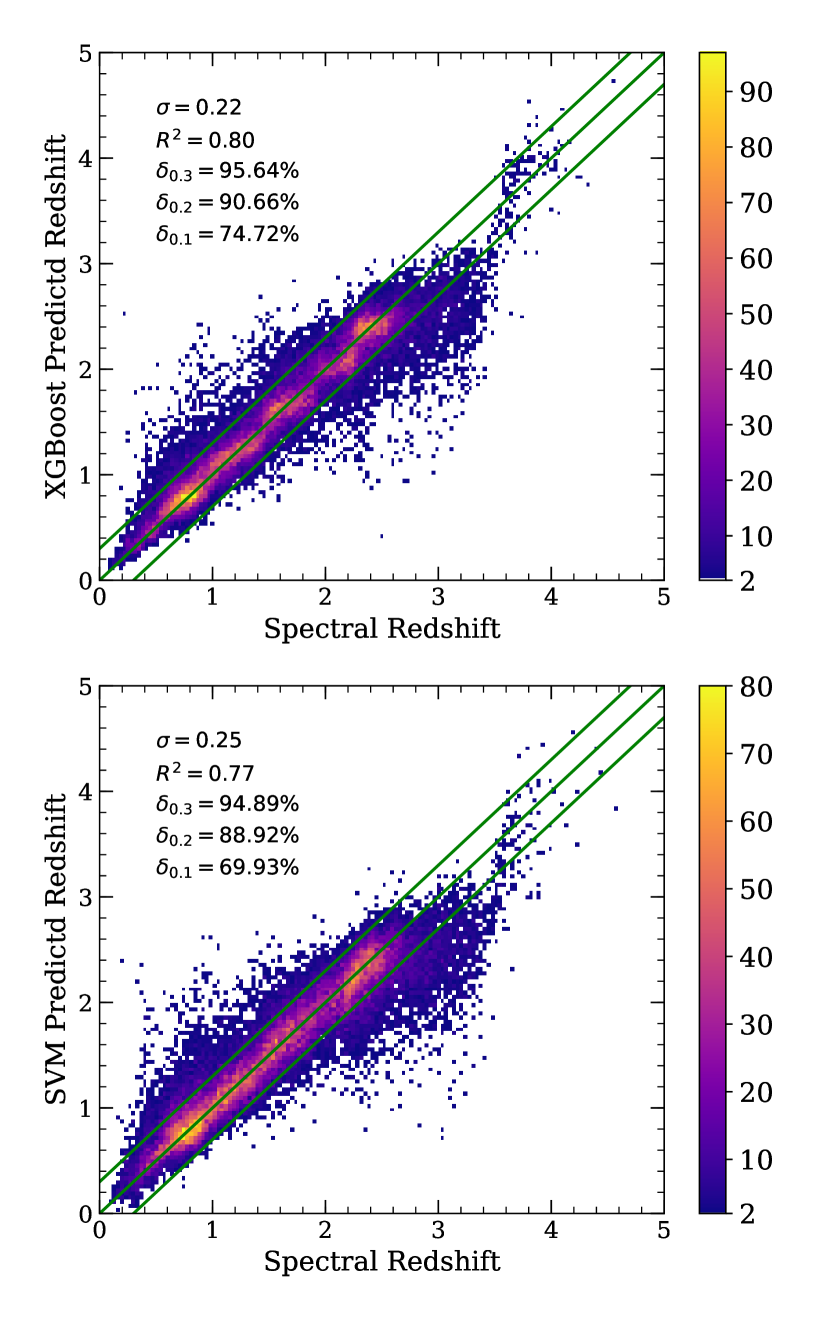
Figure 4: The estimated redshift by XGBoost and SVM regression against spectral redshift on our test set with 8Color. The color bar shows the density distribution and gives the number in each square bin. The three lines represent the diagonal of $\bigtriangleup z=0$ and the boundary of $\bigtriangleup z=0.3$

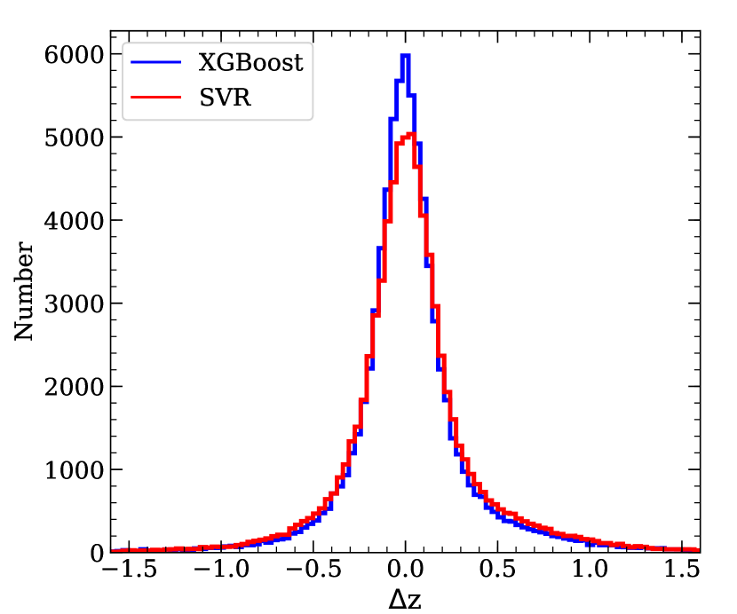
Figure 5: Distribution of the difference between the spectroscopic redshifts and estimated redshifts $\triangle z=z_{\mathrm{spec}}-z_{\mathrm{reg}}$ for XGboost and SVM on the test quasar sample.

As a result, we choose the XGBoost method to estimate the photometric redshifts of the new quasar candidates with 8Color as input pattern. In order to investigate the redshift distribution of the new quasar candidates, we adopt Richards’s criterion to divide quasars into three subgroups according to the reshift intervals $z\leq 2.2$, $2.2<z\leq 3.5$ and $3.5<z\leq 5$ (Richards et al., 2009). Table 7 lists the count of quasar candidates in different probabilities and redshift intervals. As shown in Table 7, only considering the probability $P_{\mathrm{QSO}}>0.95$, the number of low redshift, medium redshift and high redshift quasar candidates is 963,628, 230,181 and 7,402, respectively, when the magnitude $r<20$, the number of these candidates is separately 324,934, 62,674 and 2,600. The number of different redshift quasar candidates is apparently different, of which the number of higher redshift quasars is comparatively smaller. This is consistent with the fact that higher redshift quasars are too much fainter to be observed. For simplification, we only probe the redshift distribution and space distribution of quasar candidates with $P_{\mathrm{QSO}}>0.95$ of intersected results predicted by XGBoost and SVM classifiers in Figures 6-7. Figure 6 describes the redshift distribution of different samples, i.e., spectroscopic redshift distribution of known SDSS quasar sample, photometric redshift distribution of the quasar candidates. It is found that the number of our newly predicted quasar candidates in the redshift range from 0.6 to 2.6 is much larger than that of known SDSS identified quasars while the candidates with high redshift $z>2.6$ are comparable to those of SDSS. Nevertheless, it is also noted here that the SDSS/BOSS spectroscopic survey covers about 10,000 deg², whereas our candidate sample covers about 30,000 deg². In order to learn the space distribution of quasar candidates, we plot the quasar candidates in the Galactic locations in Figure 7. As shown in Figure 7, the most of quasar candidates occupy the Galactic medium latitude and are far away from the Galactic plane while only small quantity of them focus on the Galactic plane.

Table 7: Quasar candidates in different redshift intervals

	$P_{\mathrm{QSO}}>0.5$	$P_{\mathrm{QSO}}>0.75$	$P_{\mathrm{QSO}}>0.95$
$z\leq 2.2$	1,323,485	1,187,900	963,628
$2.2<z\leq 3.5$	617,536	436,811	230,181
$z>3.5$	65,611	33,277	7,402
Total No.	2,006,632	1,657,988	1,201,211
when $r<20$
$z\leq 2.2$	342,912	337,198	324,934
$2.2<z\leq 3.5$	147,354	102,963	62,674
$3.5<z\leq 5$	16,502	8,354	2,600
Total No.	506,768	448,515	390,208

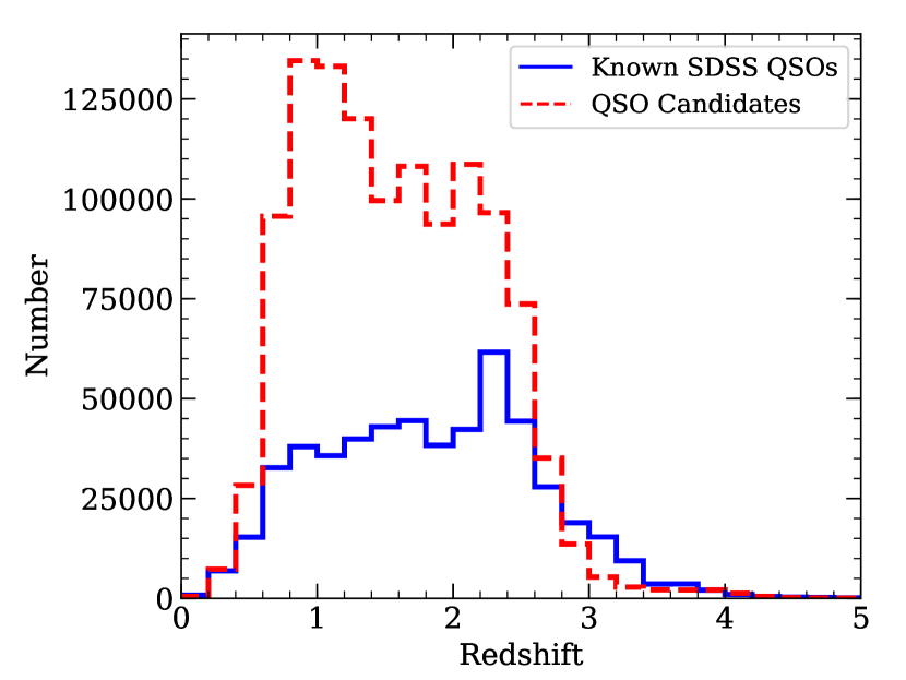
Figure 6: Redshift distribution for different samples, solid line for the whole known SDSS quasars covering about 10,000 deg², dashed line for the newly predicted quasar candidates with $P_{\mathrm{QSO}}>0.95$ covering about 30,000 deg².

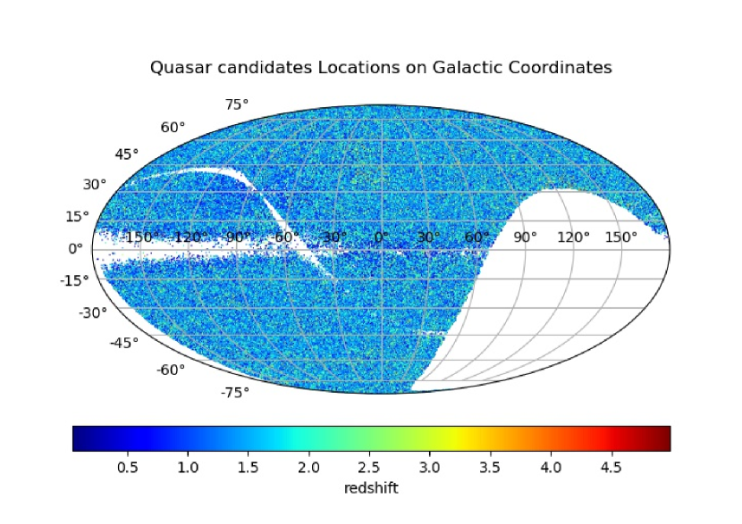
Figure 7: The distribution of quasar candidates with $P_{\mathrm{QSO}}>0.95$ on Galactic locations

5.3 Application of Quasar Candidates

Through the above experiments, Table 7 further indicates those quasar candidates by XGB$\cap$SVM in different probabilities and redshift intervals. Therefore we may choose appropriate quasar candidates for follow-up observation according to the observation condition and telescope sites.

The Large Sky Area Multi-Object Fibre Spectroscopic Telescope (LAMOST; Cui et al. 2012) is a 4-meter class reflecting Schmidt telescope with 20 square degree field of view (FOV) and 4,000 fibres, located at the Xinglong Station of National Astronomical Observatories of Chinese Academy of Sciences. It has the ability to obtain spectra of celestial objects with great efficiency. LAMOST has launched five spectroscopic surveys up to now, and the sixth spectroscopic survey is in progress. In the past five years, about 50,000 quasars were identified. For more efficient identification of quasars, careful preparation of the quasar input catalogue for LAMOST is important. In Table 7, we focus on the quasar candidates with the probability $P_{\mathrm{QSO}}>0.95$. These quasar candidates will be added into the LAMOST quasar input catalogue and greatly enriches it. Considering the magnitude limitation ($r$ magnitude less than 20) and telescope site (declination larger than $-10$), 269,121 candidates with $P_{\mathrm{QSO}}>0.95$ are kept. Among them, 1,649 have predicted redshift ($z>3.5$), 40,624 have predicted redshift ($2.2<z\leq 3.5$) and 226,848 quasars have redshift ($z\leq 2.2$).

6 Conclusion

We cross-match the Pan-STARRS1 MeanObject table with AllWISE to obtain the sources containing optical and infrared photometric information. Then we put forward color criterions and a new schema to select quasar candidates. Our experimental results show that quasar candidates can be selected very efficiently by color criterions and machine learning algorithms based on optical and infrared photometric information. According to the color criterions (yW1W2 and iW1zW2), most stellar pollution is excluded and most quasars are included. Therefore the optical and infrared color criterions are rather efficient and convenient methods to select quasar candidates. Although these techniques have such goodness, they don’t consider all known information. If using all information or in higher dimensional spaces, the efficiency will improve. Therefore using all the features from optical and infrared bands as input patterns, we build two machine learning classifiers (XGBoost and SVM) to select quasar candidates. These two classifiers behave very well in the quasar and star classification, with accuracy of more than $99.46\%$ to the flux limits of the training set (see Figure 1). Applying the classifiers to the unknown cross-matched data set, a total of 2,006,632 sources ($P_{\mathrm{QSO}}>0.5$) are predicted to be quasar candidates. Among them, 1,657,988 have the probabilities $P_{\mathrm{QSO}}>0.75$ and 1,201,211 have much higher probabilities $P_{\mathrm{QSO}}>0.95$.

By comparing the performance of photometric redshift estimation of XGBoost with that of SVM, XGBoost is superior to SVM, at least to the flux limits of the training set. Then XGBoost is adopted as the core algorithm to predict photometric redshifts of the selected quasar candidates. Using the XGBoost regression, we estimate photometric redshift for each quasar candidate. In those quasars with high probability ($P_{\mathrm{QSO}}>0.95$), 7,402 are predicted to have high redshift ($z>3.5$), 230,181 quasars have medium redshift ($2.2<z\leq 3.5$) and 963,628 quasars have low redshift ($z\leq 2.2$). Under the observation requirements of LAMOST ($r<20$, Dec $>-10$), 1,649 have predicted redshifts ($z>3.5$), 40,624 quasars with redshifts ($2.2<z\leq 3.5$) and 226,848 quasars with redshifts ($z\leq 2.2$). These candidates will be added into the input catalogue of the LAMOST telescope to identify new quasars.

In summary, the color-cuts and the new scheme we put forward to pick out quasar candidates are reliable and efficient to the flux limits of the training set. The information added from infrared band is of great value to select quasar candidates, especially high redshift quasars. Our selected quasar candidates can be observed by the LAMOST telescope or other large telescopes. In the following research, we will consider time series information from GAIA, Pan-STARRS or future LSST to select quasar candidates.

References

- Antonucci (1993) Antonucci R., 1993, ARA&A, 31, 473
- Assef et al. (2013) Assef R. J., et al., 2013, ApJ, 772, 26
- Ball et al. (2007) Ball N. M., Brunner R. J., Myers A. D., Strand N. E., Alberts S. L., Tcheng D., Llorà X., 2007, ApJ, 663, 774
- Bethapudi & Desai (2018) Bethapudi S., Desai S., 2018, Astronomy and Computing, 23, 15
- Bovy et al. (2011) Bovy J., et al., 2011, ApJ, 729, 141
- Bu et al. (2014) Bu Y., Chen F., Pan J., 2014, New Astron., 28, 35
- Budavári et al. (2001) Budavári T., et al., 2001, AJ, 122, 1163
- Butler & Bloom (2011) Butler N. R., Bloom J. S., 2011, AJ, 141, 93
- Chambers et al. (2016) Chambers K. C., et al., 2016, preprint, (arXiv:1612.05560)
- Chen & Guestrin (2016) Chen T., Guestrin C., 2016, in Acm Sigkdd International Conference on Knowledge Discovery and Data Mining.
- Croom et al. (2004) Croom S. M., Smith R. J., Boyle B. J., Shanks T., Miller L., Outram P. J., Loaring N. S., 2004, MNRAS, 349, 1397
- Cui et al. (2012) Cui X.-Q., et al., 2012, Research in Astronomy and Astrophysics, 12, 1197
- D’Abrusco et al. (2009) D’Abrusco R., Longo G., Walton N. A., 2009, MNRAS, 396, 223
- Dawson et al. (2013) Dawson K. S., et al., 2013, AJ, 145, 10
- Dawson et al. (2016) Dawson K. S., et al., 2016, AJ, 151, 44
- Fan (2006) Fan X., 2006, New Astron. Rev., 50, 665
- Fan et al. (1999) Fan X., et al., 1999, AJ, 118, 1
- Friedman (2001) Friedman J. H., 2001, Annals of Statistics, 29, 1189
- Gao et al. (2008) Gao D., Zhang Y.-X., Zhao Y.-H., 2008, MNRAS, 386, 1417
- Graham et al. (2014) Graham M. J., Djorgovski S. G., Drake A. J., Mahabal A. A., Chang M., Stern D., Donalek C., Glikman E., 2014, MNRAS, 439, 703
- Han et al. (2016) Han B., Ding H.-P., Zhang Y.-X., Zhao Y.-H., 2016, Research in Astronomy and Astrophysics, 16, 74
- Hernitschek et al. (2016) Hernitschek N., et al., 2016, ApJ, 817, 73
- Khorunzhev et al. (2016) Khorunzhev G. A., Burenin R. A., Meshcheryakov A. V., Sazonov S. Y., 2016, Astronomy Letters, 42, 277
- Kim et al. (2011) Kim D.-W., Protopapas P., Alcock C., Byun Y.-I., Khardon R., 2011, in Evans I. N., Accomazzi A., Mink D. J., Rots A. H., eds, Astronomical Society of the Pacific Conference Series Vol. 442, Astronomical Data Analysis Software and Systems XX. p. 447
- Kirkpatrick et al. (2011) Kirkpatrick J. A., Schlegel D. J., Ross N. P., Myers A. D., Hennawi J. F., Sheldon E. S., Schneider D. P., Weaver B. A., 2011, ApJ, 743, 125
- Kormendy & Ho (2013) Kormendy J., Ho L. C., 2013, ARA&A, 51, 511
- Liu et al. (2018) Liu Z.-b., Zhou F.-x., Qin Z.-t., Luo X.-g., Zhang J., 2018, Ap&SS, 363, 140
- MacLeod et al. (2011) MacLeod C. L., et al., 2011, ApJ, 728, 26
- Maddox et al. (2012) Maddox N., Hewett P. C., Péroux C., Nestor D. B., Wisotzki L., 2012, MNRAS, 424, 2876
- McGreer et al. (2009) McGreer I. D., Helfand D. J., White R. L., 2009, AJ, 138, 1925
- Mirabal et al. (2016) Mirabal N., Charles E., Ferrara E. C., Gonthier P. L., Harding A. K., Sánchez-Conde M. A., Thompson D. J., 2016, ApJ, 825, 69
- Mortlock et al. (2011) Mortlock D. J., et al., 2011, Nature, 474, 616
- Myers et al. (2015) Myers A. D., et al., 2015, ApJS, 221, 27
- Nakos et al. (2009) Nakos T., et al., 2009, A&A, 494, 579
- Palanque-Delabrouille et al. (2016a) Palanque-Delabrouille N., et al., 2016a, A&A, 587, A41
- Palanque-Delabrouille et al. (2016b) Palanque-Delabrouille N., et al., 2016b, A&A, 589, C2
- Pâris et al. (2017) Pâris I., et al., 2017, A&A, 597, A79
- Pâris et al. (2018) Pâris I., et al., 2018, A&A, 613, A51
- Pedregosa et al. (2011) Pedregosa F., et al., 2011, Journal of Machine Learning Research, 12, 2825
- Peng et al. (2012) Peng N., Zhang Y., Zhao Y., Wu X.-b., 2012, MNRAS, 425, 2599
- Peters et al. (2015) Peters C. M., et al., 2015, ApJ, 811, 95
- Reyes et al. (2008) Reyes R., et al., 2008, AJ, 136, 2373
- Richards et al. (2001) Richards G. T., et al., 2001, AJ, 122, 1151
- Richards et al. (2004) Richards G. T., et al., 2004, ApJS, 155, 257
- Richards et al. (2009) Richards G. T., et al., 2009, ApJS, 180, 67
- Ross et al. (2012) Ross N. P., et al., 2012, ApJS, 199, 3
- Schindler et al. (2017) Schindler J.-T., Fan X., McGreer I. D., Yang Q., Wu J., Jiang L., Green R., 2017, ApJ, 851, 13
- Schlafly & Finkbeiner (2011) Schlafly E. F., Finkbeiner D. P., 2011, ApJ, 737, 103
- Schmidt (1963) Schmidt M., 1963, Nature, 197, 1040
- Schneider et al. (2010) Schneider D. P., et al., 2010, AJ, 139, 2360
- Sreejith et al. (2018) Sreejith S., et al., 2018, MNRAS, 474, 5232
- Stern et al. (2012) Stern D., et al., 2012, ApJ, 753, 30
- Tuccillo et al. (2015) Tuccillo D., González-Serrano J. I., Benn C. R., 2015, MNRAS, 449, 2818
- Vapnik (1995) Vapnik V. N., 1995, The Nature of Statistical Learning Theory. Springer,
- Wang et al. (2008) Wang D., Zhang Y., Zhao Y., 2008, in Argyle R. W., Bunclark P. S., Lewis J. R., eds, Astronomical Society of the Pacific Conference Series Vol. 394, Astronomical Data Analysis Software and Systems XVII. p. 509
- Wang et al. (2016) Wang F., et al., 2016, ApJ, 819, 24
- Weinstein et al. (2004) Weinstein M. A., et al., 2004, ApJS, 155, 243
- Worseck & Prochaska (2011) Worseck G., Prochaska J. X., 2011, ApJ, 728, 23
- Wright et al. (2010) Wright E. L., et al., 2010, AJ, 140, 1868
- Wu & Jia (2010) Wu X.-B., Jia Z., 2010, MNRAS, 406, 1583
- Yang et al. (2017) Yang Q., et al., 2017, AJ, 154, 269
- Yèche et al. (2010) Yèche C., et al., 2010, A&A, 523, A14
- York et al. (2000) York D. G., et al., 2000, The Astronomical Journal, 120, 1579
- Zakamska et al. (2003) Zakamska N. L., et al., 2003, AJ, 126, 2125
- Zhang & Zhao (2003) Zhang Y., Zhao Y., 2003, PASP, 115, 1006
- Zhang & Zhao (2004) Zhang Y., Zhao Y., 2004, A&A, 422, 1113
- Zhang et al. (2011) Zhang Y., Zhao Y., Peng N., 2011, in Evans I. N., Accomazzi A., Mink D. J., Rots A. H., eds, Astronomical Society of the Pacific Conference Series Vol. 442, Astronomical Data Analysis Software and Systems XX. p. 123