Master Majorana neutrino mass parametrization

Abstract

After showing that the neutrino mass matrix in all Majorana models can be described by a general master formula, we will present a master parametrization for the Yukawa matrices, also valid for all Majorana models, that automatically ensures agreement with neutrino oscillation data. The application of the master parametrization will be illustrated in an example model.

1 Introduction

The existence of non-zero neutrino masses is nowadays an established experimental fact that calls for an extension of the Standard Model (SM) of particle physics. In fact, many neutrino mass models have been proposed, see [1, 2, 3, 4, 5, 6, 7] for some recent reviews and classification papers.

Here we will concentrate on Majorana neutrino mass models. We will first show that in this class of models the neutrino mass matrix can always be regarded as a particular case of a master formula. This general expression is written in terms of generic mass and Yukawa matrices which take specific forms in a given model. We will then enforce the agreement with neutrino oscillation data by introducing a master parametrization of the Yukawa matrices appearing in this formula. In order to illustrate the application of this parametrization we will consider an example in the BNT model [8], a model that requires one to use the full power of the master parametrization. For more details on the master formula and parametrization, we refer to [9] as well as to the extended work [10].

2 The master formula

A Majorana neutrino mass matrix can always be written as

$$m=f\,\left(y_{1}^{T}\,M\,y_{2}+y_{2}^{T}\,M^{T}\,y_{1}\right)\,.$$ (1)

Here $m$ is the neutrino mass matrix, a $3\times 3$ complex symmetric matrix that can be diagonalized as

$$D_{m}=\text{diag}\left(m_{1},m_{2},m_{3}\right)=U^{T}\,m\,U\,,$$ (2)

with $U$ a $3\times 3$ unitary matrix. $y_{1}$ and $y_{2}$ are two general $n_{1}\times 3$ and $n_{2}\times 3$ complex Yukawa matrices, respectively, and $M$ is a $n_{1}\times n_{2}$ complex matrix with dimension of mass. In the following we will assume $n_{1}\geq n_{2}$. Since $m$ must contain at least two non-vanishing eigenvalues in order to accommodate the solar and atmospheric mass scales, $r_{m}=\text{rank}(m)=2\,\text{or}\,3$.

Eq. (1) is a master formula valid for all Majorana neutrino mass models. In fact, the resulting neutrino mass matrices in specific models can be seen as particular cases of this general expression. Let us consider three examples:

• In the type-I seesaw with $3$ generations of right-handed neutrinos, the light neutrino mass matrix is given by the well-known seesaw formula, $m=-\langle H^{0}\rangle^{2}\,y^{T}M_{R}^{-1}y$. This can be obtained with the master formula by taking $n_{1}=n_{2}=3$ and the specific values $f=-1$, $y_{1}=y_{2}=y/\sqrt{2}$ and $M=\langle H^{0}\rangle^{2}\,M_{R}^{-1}$, with $\langle H^{0}\rangle=v/\sqrt{2}$ the SM Higgs ($H$) vacuum expectation value (VEV) and $M_{R}$ the Majorana mass matrix for the right-handed neutrinos.

• The inverse seesaw [11] would correspond to the same $y_{1,2}=y$ and $f$ values, but $M=\langle H^{0}\rangle^{2}\,(M_{R}^{T})^{-1}\mu M_{R}^{-1}$, with $\mu$ the small lepton number violating parameter.

• In the scotogenic model [12], the neutrino mass matrix is induced at the 1-loop level and can also be seen as a particular case of the general master formula. It corresponds to $f=\lambda_{5}/(16\pi^{2})$ and $M=\langle H^{0}\rangle^{2}\,M_{R}^{-1}F_{\rm loop}$, with $\lambda_{5}\,(H^{\dagger}\eta)^{2}$ the quartic term involving the usual and inert ($\eta$) scalar doublets, and $F_{\rm loop}$ a matrix containing loop functions.

Finally, a non-trivial example with with $y_{1}\neq y_{2}$ will be considered in Sec. 4.

3 The master parametrization

In order to guarantee consistency with neutrino oscillation data, the Yukawa matrices $y_{1}$ and $y_{2}$ in Eq. (1) can be written as

$$y_{1} =\frac{1}{\sqrt{2\,f}}\,V_{1}^{\dagger}\,\left(\begin{array}[]{c}\Sigma^{-1/2}\,W\,A\\ X_{1}\\ X_{2}\end{array}\right)\,\bar{D}_{\sqrt{m}}\,U^{\dagger}\,,$$ (6)

$$y_{2} =\frac{1}{\sqrt{2\,f}}\,V_{2}^{\dagger}\,\left(\begin{array}[]{c}\Sigma^{-1/2}\,\widehat{W}^{\ast}\,\widehat{B}\\ X_{3}\end{array}\right)\,\bar{D}_{\sqrt{m}}\,U^{\dagger}\,.$$ (9)

This is the master parametrization. We now proceed to define the matrices that appear in Eqs. (6) and (9). First, we have introduced the diagonal matrix $\bar{D}_{\sqrt{m}}$, given by diag$\left(\sqrt{m_{1}},\sqrt{m_{2}},\sqrt{m_{3}}\right)$ if $r_{m}=3$ or diag$\left(\sqrt{m_{1}},\sqrt{m_{2}},\sqrt{v}\right)$ if $r_{m}=2$. The matrix $M$ has been singular-value decomposed as

$$M=V_{1}^{T}\,\widehat{\Sigma}\,V_{2}\,,$$ (10)

where $\widehat{\Sigma}$ is a $n_{1}\times n_{2}$ matrix that can be written as

$$\widehat{\Sigma}=\left(\begin{array}[]{c}\begin{array}[]{cc}\Sigma&0\\ 0&0_{n_{2}-n}\end{array}\\ \hline\cr 0_{n_{1}-n_{2}}\end{array}\right)\,,$$ (11)

and $\Sigma=\text{diag}\left(\sigma_{1},\sigma_{2},\dots,\sigma_{n}\right)$ is the diagonal $n\times n$ matrix that contains the positive and real singular values of $M$ ($\sigma_{i}>0$). $V_{1}$ and $V_{2}$ are two unitary matrices, with dimensions $n_{1}\times n_{1}$ and $n_{2}\times n_{2}$, respectively. $X_{1}$, $X_{2}$ and $X_{3}$ are three arbitrary complex matrices with dimensions $(n_{2}-n)\times 3$, $(n_{1}-n_{2})\times 3$ and $(n_{2}-n)\times 3$, respectively, and whose entries have dimensions of mass^-1/2. $\widehat{W}$ is an $n\times n$ matrix defined as

$$\widehat{W}=\left(W\quad\bar{W}\right)\,,$$ (12)

where $W$ is an $n\times r$ complex matrix, such that $W^{\dagger}W=W^{T}W^{*}=\mathbb{I}_{r}$. Here we have defined $r=\text{rank}(W)$. The matrix $\bar{W}$ is an $n\times(n-r)$ complex matrix, built with vectors that complete those in $W$ to form an orthonormal basis of $\mathbb{C}^{n}$. Furthermore, $A$ is an $r\times 3$ matrix that can be expressed as

$$A=T\,C_{1}\,,$$ (13)

with $T$ an upper-triangular $r\times r$ invertible square matrix with $T_{ii}>0$, and $C_{1}$ is an $r\times 3$ matrix. Finally, $\widehat{B}$ is an $n\times 3$ complex matrix, which can be written in blocks as

$$\widehat{B}=\left(\begin{array}[]{c}B\\ \bar{B}\\ \end{array}\right)\,,$$ (14)

with $\bar{B}$ an arbitrary $(n-r)\times 3$ complex matrix and $B$ an $r\times 3$ complex matrix given by

$$B\equiv B\left(T,K,C_{1},C_{2}\right)=\left(T^{T}\right)^{-1}\,\left[C_{1}\,C_{2}+K\,C_{1}\right]\,.$$ (15)

In the last equation we have introduced the antisymmetric $r\times r$ square matrix $K$ and the $3\times 3$ matrix $C_{2}$. The form of the matrices $C_{1}$ and $C_{2}$ depends on the ranks $r_{m}$ and $r$ (see [10] for all the expressions). For instance, for $r_{m}=r=3$ these matrices are given by

$$C_{1}=\mathbb{I}_{3},\quad C_{2}=\mathbb{I}_{3}+K_{12}\,\frac{T_{13}}{T_{11}}\,\left(\begin{array}[]{ccc}0&0&0\\ 0&0&1\\ 0&-1&0\end{array}\right)\,.$$ (19)

The use of the master parametrization might look complicated but is actually straightforward. The first step is to use information from neutrino oscillation experiments (typically from a global fit) to fix the light neutrino masses and leptonic mixing angles appearing in $\bar{D}_{\sqrt{m}}$ and $U$, respectively. Next, one must compare the expression for the neutrino mass matrix in the specific model under study with the general master formula in Eq. (1). This way one identifies the global factor $f$, the Yukawa matrices $y_{1}$ and $y_{2}$ and the matrix $M$, and by singular-value decomposing the latter one determines $\Sigma$, $V_{1}$ and $V_{2}$. Finally, one can randomly scan over the free parameters contained in the matrices $\widehat{W}$, $X_{1,2,3}$, $\bar{B}$, $T$, $K$ and $C_{1,2}$ to compute the Yukawa matrices $y_{1}$ and $y_{2}$ by means of Eqs. (6) and (9).

Let us now compare to the Casas-Ibarra parametrization [13]. As explained above, the master parametrization can be applied to any Majorana neutrino mass model, while the use of the Casas-Ibarra parametrization is restricted to the type-I seesaw (and similar models). Therefore, they should agree in that case. First, we remind the reader that comparing the neutrino mass matrix in this model to our master formula one finds $y_{1}=y_{2}=y/\sqrt{2}$, $n_{1}=n_{2}=n=r=3$, $f=-1$ and $M=\langle H^{0}\rangle^{2}M_{R}^{-1}$. Since $M$ is symmetric, it can be diagonalized by a single matrix, and hence $V_{1}=V_{2}$. Moreover, this matrix can be taken to be the identity when the right-handed neutrinos are given in their mass basis. Finally, since $n_{1}=n_{2}=n=r=3$ the matrices $X_{1,2,3}$, $\overline{W}$ and $\overline{B}$ just drop from all the expressions. The condition $y_{1}=y_{2}$ can be shown to be equivalent to $W^{T}WA=B$, which in turn leads to $B=\left(A^{T}\right)^{-1}$ and $R=W\,A$, with $R$ a $3\times 3$ orthogonal matrix. With these ingredients at hand one can simply use Eqs. (6) and (9) to find

$$y=\sqrt{2}\,y_{1}=\sqrt{2}\,y_{2}=i\,\Sigma^{-1/2}\,R\,D_{\sqrt{m}}\,U^{\dagger}\,,$$ (20)

which, after identifying $R$ with the usual Casas-Ibarra matrix, is nothing but the Casas-Ibarra parametrization [13]. Therefore, we see that the Casas-Ibarra parametrization can be interpreted as a particular case of the master parametrization.

4 An example application

Finally, we would like to show an application of the master parametrization to the BNT model [8]. The particle content of this model includes three generations of the vector-like fermions $\psi_{L,R}$, which transform as $({\bf 1},{\bf 3},-1)$ under the SM gauge group and the scalar $\Phi$, which transfors as $({\bf 1},{\bf 4},3/2)$. The quantum numbers of the new particles in the BNT model are given in Table 1.

	generations	$\mathrm{SU(3)}_{c}$	$\mathrm{SU(2)}_{L}$	$\mathrm{U(1)}_{Y}$
$\Phi$	1	${\bf 1}$	${\bf 4}$	$3/2$
$\psi_{L,R}$	3	${\bf 1}$	${\bf 3}$	$-1$

Table 1: New particles in the BNT model.

The Lagrangian contains the following terms

$$-\mathcal{L} \supset y_{\psi}\,\overline{L}\,H\,\psi_{R}+y_{\bar{\psi}}\,\overline{L^{c}}\,\Phi\,\psi_{L}+M_{\psi}\overline{\psi}\,\psi+\lambda_{\Phi}\,H^{3}\,\Phi^{\dagger}+\mathrm{h.c.}\,,$$ (21)

where we have omitted gauge and flavor indices for the sake of clarity. In the presence of a non-zero $\lambda_{\Phi}$ coupling the model breaks lepton number in two units and induces neutrino masses as shown in Fig. 1. The resulting neutrino mass matrix is given by

$$m=\frac{\lambda_{\Phi}v^{4}}{4M_{\Phi}^{2}}\,\left[y_{\psi}^{T}\,M_{\psi}^{-1}\,y_{\bar{\psi}}+y_{\bar{\psi}}^{T}\,(M_{\psi}^{-1})^{T}\,y_{\psi}\right]\,.$$ (22)

Furthermore, the $\lambda_{\Phi}$ term induces a non-zero VEV for the neutral component of $\Phi$, $\Phi^{0}$,

$$\langle\Phi^{0}\rangle=\frac{v_{\Phi}}{\sqrt{2}}=\frac{\lambda_{\Phi}v^{3}}{2\sqrt{2}M_{\Phi}^{2}}\,.$$ (23)

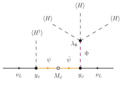
Figure 1: Neutrino mass generation in the BNT model.

One cannot apply the Casas-Ibarra parametrization in the BNT model since one has two independent $y_{1}=y_{\psi}$ and $y_{2}=y_{\bar{\psi}}$ Yukawa matrices. Therefore, the master parametrization is required in order to guarantee consistency with neutrino oscillation experiments. First, we compare to Eq. (1) and identify

$$f=\frac{\lambda_{\Phi}v^{2}}{2M_{\Phi}^{2}}\,,\quad M=\frac{v^{2}}{2}\,M_{\psi}^{-1}\,.$$ (24)

Moreover, the matrices $y_{1}$, $y_{2}$ and $M$ are $3\times 3$ in this model and then $n_{1}=n_{2}=3$. One also has $n=3$ and $\widehat{\Sigma}\equiv\Sigma$. Finally, we consider the choice $r=r_{m}=3$, implying that the matrices $X_{1,2,3}$ and $\bar{B}$ are absent, while $C_{1}$ and $C_{2}$ are given in Eq. (19).

We have performed numerical scans to show the usefulness of the master parametrization. In order to do that we have made use of the neutrino oscillation parameters derived by the global fit [14], implemented the model in SARAH [15] and obtained numerical results with SPheno [16]. We show a selected result on the lepton flavor violating observable Br$(\mu\to e\gamma)$, computed with the FlavorKit package [17], in Fig. 2. This figure serves to illustrate a crucial point when running a numerical scan. One can take simple forms for the matrices that appear in the master parametrization (for instance, $T=\mathbb{I}$ or $K=0$). However, that would cover a limited region of the parameter space of the model, potentially leading to fictitious correlations that get broken in other parameter regions. Fig. 2 precisely shows the results of a random scan with or without using the freedom in the matrices $T$ and $K$. The correlation that would be found in the simplified scan (in black) is not found in a more general exploration (in purple). Thanks to the master parametrization one can run completely general scans and avoid finding this sort of fake correlations.

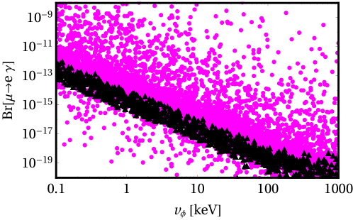
Figure 2: Br$(\mu\to e\gamma)$ as a function of $v_{\Phi}$ in the BNT model. Neutrino oscillation parameters are allowed to vary within the 3 $\sigma$ ranges determined in [14], assuming normal hierarchy. $M_{\Psi}$ has been randomly taken in the interval $[0.5,2]$ TeV and $W$ fixed to the identity matrix. The purple points correspond to a scan in which the elements of the matrices $T$ and $K$ are randomly taken in the following ranges: $T_{ii}\in[0,2]$ and $K_{ij}$, $T_{ij}$ (with $i\neq j$) $\in[-1,1]$. The black points correspond to a simplified scan with $T=\mathbb{I}$ and $K=0$.

5 Summary

The master parametrization [9] can be applied to any Majorana neutrino mass model and allows one to explore its parameter space in a complete way and in full agreement with neutrino oscillation data. Here we have detailed its ingredients and illustrated its use for the particular case of the BNT model. Given the large number of Majorana mass models in the literature, the master parametrization constitutes a useful and general tool that allows one to run systematic and automatizable phenomenological analyses in a wide variety of scenarios beyond the SM.

Acknowledgements

Work supported by the Spanish grants AYA2015-66899-C2-1-P, SEV-2014-0398 and FPA2017-85216-P (AEI/FEDER, UE), PROMETEO/2018/165 and SEJI/2018/033 (Generalitat Valenciana) and the Spanish Red Consolider MultiDark FPA2017-90566-REDC.

References

References

- [1] Ma E and Popov O 2017 Phys. Lett. B764 142–144 (Preprint 1609.02538)
- [2] Centelles Chuliá S, Srivastava R and Valle J W F 2018 Phys. Lett. B781 122–128 (Preprint 1802.05722)
- [3] Ma E 1998 Phys. Rev. Lett. 81 1171–1174 (Preprint hep-ph/9805219)
- [4] Cai Y, Herrero-García J, Schmidt M A, Vicente A and Volkas R R 2017 Front.in Phys. 5 63 (Preprint 1706.08524)
- [5] Cepedello R, Fonseca R M and Hirsch M 2018 JHEP 10 197 (Preprint 1807.00629)
- [6] Boucenna S M, Morisi S and Valle J W F 2014 Adv. High Energy Phys. 2014 831598 (Preprint 1404.3751)
- [7] Anamiati G, Castillo-Felisola O, Fonseca R M, Helo J C and Hirsch M 2018 JHEP 12 066 (Preprint 1806.07264)
- [8] Babu K S, Nandi S and Tavartkiladze Z 2009 Phys. Rev. D80 071702 (Preprint 0905.2710)
- [9] Cordero-Carrión I, Hirsch M and Vicente A 2018 (Preprint 1812.03896)
- [10] Cordero-Carrión I, Hirsch M and Vicente A (in preparation)
- [11] Mohapatra R N and Valle J W F 1986 Phys. Rev. D34 1642
- [12] Ma E 2006 Phys. Rev. D73 077301 (Preprint hep-ph/0601225)
- [13] Casas J A and Ibarra A 2001 Nucl. Phys. B618 171–204 (Preprint hep-ph/0103065)
- [14] de Salas P F, Forero D V, Ternes C A, Tortola M and Valle J W F 2018 Phys. Lett. B782 633–640 (Preprint 1708.01186)
- [15] Staub F 2014 Comput. Phys. Commun. 185 1773–1790 (Preprint 1309.7223)
- [16] Porod W and Staub F 2012 Comput. Phys. Commun. 183 2458–2469 (Preprint 1104.1573)
- [17] Porod W, Staub F and Vicente A 2014 Eur. Phys. J. C74 2992 (Preprint 1405.1434)