Fast Multichannel Source Separation Based on Jointly Diagonalizable Spatial Covariance Matrices

Abstract

This paper describes a versatile method that accelerates multichannel source separation methods based on full-rank spatial modeling. A popular approach to multichannel source separation is to integrate a spatial model with a source model for estimating the spatial covariance matrices (SCMs) and power spectral densities (PSDs) of each sound source in the time-frequency domain. One of the most successful examples of this approach is multichannel nonnegative matrix factorization (MNMF) based on a full-rank spatial model and a low-rank source model. MNMF, however, is computationally expensive and often works poorly due to the difficulty of estimating the unconstrained full-rank SCMs. Instead of restricting the SCMs to rank-1 matrices with the severe loss of the spatial modeling ability as in independent low-rank matrix analysis (ILRMA), we restrict the SCMs of each frequency bin to jointly-diagonalizable but still full-rank matrices. For such a fast version of MNMF, we propose a computationally-efficient and convergence-guaranteed algorithm that is similar in form to that of ILRMA. Similarly, we propose a fast version of a state-of-the-art speech enhancement method based on a deep speech model and a low-rank noise model. Experimental results showed that the fast versions of MNMF and the deep speech enhancement method were several times faster and performed even better than the original versions of those methods, respectively.

I Introduction

Multichannel source separation plays a central role for computational auditory scene analysis. To make effective use of an automatic speech recognition system in a noisy environment, for example, it is indispensable to separate speech signals from noise-contaminated signals. A standard approach to multichannel source separation is to use a non-blind method (e.g., beamforming and Wiener filtering) based on the spatial covariance matrix (SCM) of a target source (e.g., speech) and those of the other sources (e.g., noise). To use beamforming for speech enhancement, deep neural networks (DNNs) are often used for classifying each time-frequency bin into speech or noise [1, 2, 3]. The performance of such a supervised approach, however, is often considerably degraded in an unseen environment. In this paper we thus focus on general-purpose blind source separation (BSS) and its extension for environment-adaptive semi-supervised speech enhancement.

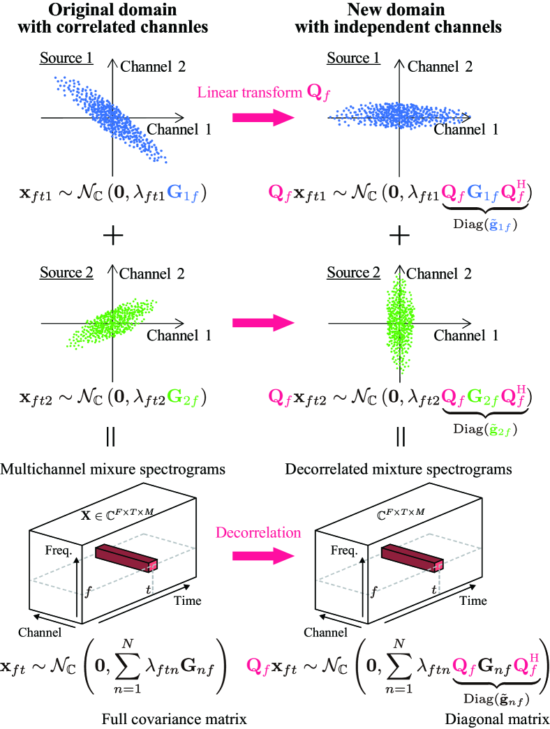
Figure 1: The full-rank spatial model for the correlated channels of the original data is equivalent to the diagonal spatial model for the independent channels of the decorrelated data.

The goal of BSS is to estimate both a mixing process and sound sources from observed mixtures. To solve such an ill-posed problem, one can take a statistical approach based on a spatial model representing a sound propagation process and a source model representing the power spectral densities (PSDs) of each source. Duong et al. [4] pioneered this approach by integrating a full-rank spatial model using the frequency-wise full-rank SCMs of each source with a source model assuming the source spectra to follow complex Gaussian distributions. We call it as full-rank spatial covariance analysis (FCA) in this paper as in [5]. To alleviate the frequency permutation problem of FCA, multichannel nonnegative matrix factorization (MNMF) that uses an NMF-based source model for representing the co-occurrence and low-rankness of frequency components has been developed [6, 7, 8]. Such a low-rank source model, however, does not fit speech spectra. In speech enhancement, a semi-supervised approach that uses as source models a DNN-based speech model (deep prior, DP) trained from clean speech data and an NMF-based noise model learned on the fly has thus recently been investigated (called MNMF-DP) [9, 10, 11].

The major drawbacks common to these methods based on the full-rank SCMs are the high computational cost due to the repeated heavy operations (e.g., inversion) of the SCMs and the difficulty of parameter optimization due to the large degree of freedom (DOF) of the spatial model. Kitamura et al. [12] thus proposed a constrained version of MNMF called independent low-rank matrix analysis (ILRMA) that restricts the SCMs to rank-1 matrices. Although ILRMA is an order of magnitude faster and practically performed better than MNMF, it suffers from the severe loss of the spatial modeling ability. Ito et al. [5] proposed a fast version of FCA that restricts the SCMs of each frequency bin to jointly-diagonalizable matrices. For parameter estimation, an expectation-maximization (EM) algorithm with a fixed-point iteration (FPI) method was proposed, but its convergence was not guaranteed.

In this paper we propose a versatile convergence-guaranteed method for estimating the jointly-diagonalizable SCMs of the full-rank spatial model and its application to FCA, MNMF, and MNMF-DP called FastFCA, FastMNMF, and FastMNMF-DP, respectively, where FastMNMF has an intermediate ability of spatial modeling between MNMF and ILRMA. As shown in Fig. 1, while all channels are correlated in the original spectrograms, they are independent in the linearly-transformed spectrograms obtained by applying a diagonalizer to each frequency bin. MNMF for the original complex spectrograms is thus equivalent to computationally-efficient nonnegative tensor factorization (NTF) for the independent nonnegative PSDs of the transformed spectrograms. To estimate such a diagonalizer (linear transform), we use an iterative projection (IP) method in a way similar to independent vector analysis (IVA) [13] that estimates a demixing matrix. The resulting algorithm based on iterations of NTF and IP is similar in form to that of ILRMA based on iterations of NMF and IP.

One of the important contributions of this paper is to improve existing decomposition methods by joint diagonalization of covariance matrices. This idea was first discussed for an ultimate but computationally-prohibitive extension of NTF called correlated tensor factorization (CTF) [14] based on multi-way full-rank covariance matrices, resulting in a fast version of CTF called independent low-rank tensor analysis (ILRTA) [15]. While ILRTA was used for single-channel BSS based on jointly-diagonalizable frequency covariance matrices, in this paper we focus on multi-channel BSS based on jointly-diagonalizable spatial covariance matrices. Since NTF and IP are used in common for parameter optimization, the proposed FastMNMF can be regarded as a special case of ILRTA.

II Multichannel Source Separation

This section reviews existing multichannel source separation methods based on a full-rank spatial model, i.e., full-rank spatial covariance analysis (FCA) [4] based on an unconstrained source model, MNMF [8] based on an NMF-based source model, and its adaptation to speech enhancement called MNMF-DP [10] based on a DNN-based speech model and an NMF-based noise model.

II-A Full-Rank Spatial Model

II-A1 Model Formulation

Suppose that $N$ sources are observed by $M$ microphones. Let $\mathbf{X}=\{\mathbf{x}_{ft}\}_{f,t=1}^{F,T}\in\mathbb{C}^{F\times T\times M}$ be the observed multichannel complex spectra, where $F$ and $T$ are the number of frequency bins and that of frames, respectively. Let $\mathbf{x}_{ftn}=[x_{ftn1},\cdots,x_{ftnM}]^{\mathrm{T}}\in\mathbb{C}^{M}$ be the image of source $n$ assumed to be circularly-symmetric complex Gaussian distributed as follows:

$$\mathbf{x}_{ftn}\sim\mathcal{N}_{\mathbb{C}}\left(\mathbf{0},\lambda_{ftn}\mathbf{G}_{nf}\right),$$ (1)

where $\lambda_{ftn}$ is the PSD of source $n$ at frequency $f$ and time $t$, $\mathbf{G}_{nf}$ is the $M\times M$ positive definite full-rank SCM of source $n$ at frequency $f$. Using the reproductive property of the Gaussian distribution, the observed spectrum $\mathbf{x}_{ft}=\sum_{n=1}^{N}\mathbf{x}_{ftn}$ is given by

$$\mathbf{x}_{ft}\sim\mathcal{N}_{\mathbb{C}}\!\left(\mathbf{0},\sum_{n=1}^{N}\lambda_{ftn}\mathbf{G}_{nf}\right).$$ (2)

Given the mixture spectrum $\mathbf{x}_{ft}$ and the model parameters $\mathbf{G}_{nf}$ and $\lambda_{ftn}$, the posterior expectation of the source image $\mathbf{x}_{ftn}$ is obtained by multichannel Wiener filtering (MWF):

$$\mathbf{x}_{ftn}=\mathbb{E}[\mathbf{x}_{ftn}|\mathbf{x}_{ft}]=\mathbf{Y}_{ftn}\mathbf{Y}_{ft}^{-1}\mathbf{x}_{ft},$$ (3)

where $\mathbf{Y}_{ftn}\!\overset{\mbox{def}}{=}\!\lambda_{ftn}\mathbf{G}_{nf}$ and $\mathbf{Y}_{ft}\!\overset{\mbox{def}}{=}\!\sum_{n=1}^{N}\!\!\mathbf{Y}_{ftn}$.

II-A2 Parameter Estimation

Our goal is to estimate the parameters $\mathbf{G}=\{\mathbf{G}_{nf}\}_{f,n=1}^{F,N}$ and $\bm{\Lambda}=\{\lambda_{ftn}\}_{f,t,n=1}^{F,T,N}$ that maximize the log-likelihood given by Eq. (2):

$$\log p({\mathbf{X}}|\mathbf{G},\bm{\Lambda})\overset{\mbox{c}}{=}-\sum_{f,t=1}^{F,T}\left(\mathrm{tr}\!\left(\mathbf{X}_{ft}\mathbf{Y}_{ft}^{-1}\right)+\log\!\left|\mathbf{Y}_{ft}\right|\right),$$ (4)

where $\mathbf{X}_{ft}\!\overset{\mbox{def}}{=}\!\mathbf{x}_{ft}\mathbf{x}_{ft}^{\mathrm{H}}$. In this paper we use a majorization-minimization (MM) algorithm [8] that iteratively maximizes a lower bound of Eq. (4). As in [14, 15], the closed-form update rule of $\mathbf{G}$ was recently found to be given by

$$\mathbf{A}_{nf} \overset{\mbox{def}}{=}\textstyle\sum_{t=1}^{T}\lambda_{ftn}\mathbf{Y}_{ft}^{-1}\mathbf{X}_{ft}\mathbf{Y}_{ft}^{-1},$$ (5)

$$\mathbf{B}_{nf} \overset{\mbox{def}}{=}\textstyle\sum_{t=1}^{T}\lambda_{ftn}\mathbf{Y}_{ft}^{-1},$$ (6)

$$\mathbf{G}_{nf} \leftarrow\mathbf{B}_{nf}^{-1}\left(\mathbf{B}_{nf}\mathbf{G}_{nf}\mathbf{A}_{nf}\mathbf{G}_{nf}\right)^{\frac{1}{2}}.$$ (7)

II-B Source Models

II-B1 Unconstrained Source Model

The unconstrained model directly uses $\bm{\Lambda}$ as free parameters. Using the MM algorithm, the multiplicative update (MU) rule of $\bm{\Lambda}$ is given by

$$\lambda_{ftn}\leftarrow\lambda_{ftn}\sqrt{\frac{\mathrm{tr}\!\left(\mathbf{G}_{nf}\mathbf{Y}_{ft}^{-1}\mathbf{X}_{ft}\mathbf{Y}_{ft}^{-1}\right)}{\mathrm{tr}\!\left(\mathbf{G}_{nf}\mathbf{Y}_{ft}^{-1}\right)}}.$$ (8)

II-B2 NMF-Based Source Model

If the PSDs $\{\lambda_{ftn}\}_{f,t=1}^{F,T}$ of a source $n$ (e.g., noise and music) have low-rank structure, the PSDs can be factorized as follows [8]:

$$\lambda_{ftn}=\sum_{k=1}^{K}w_{nkf}h_{nkt},$$ (9)

where $K$ is the number of bases, $w_{nkf}\geq 0$ is the magnitude of basis $k$ of source $n$ at frequency $f$, and $h_{nkt}\geq 0$ is the activation of basis $k$ of source $n$ at time $t$. Using the MM algorithm[16], the MU rules of $\mathbf{W}$ and $\mathbf{H}$ are given by

$$w_{nkf} \leftarrow w_{nkf}\sqrt{\frac{\sum_{t=1}^{T}h_{nkt}\,\mathrm{tr}\!\left(\mathbf{G}_{nf}\mathbf{Y}_{ft}^{-1}\mathbf{X}_{ft}\mathbf{Y}_{ft}^{-1}\right)}{\sum_{t=1}^{T}h_{nkt}\,\mathrm{tr}\!\left(\mathbf{G}_{nf}\mathbf{Y}_{ft}^{-1}\right)}},$$ (10)

$$h_{nkt} \leftarrow h_{nkt}\sqrt{\frac{\sum_{f=1}^{F}w_{nkf}\,\mathrm{tr}\!\left(\mathbf{G}_{nf}\mathbf{Y}_{ft}^{-1}\mathbf{X}_{ft}\mathbf{Y}_{ft}^{-1}\right)}{\sum_{f=1}^{F}w_{nkf}\,\mathrm{tr}\!\left(\mathbf{G}_{nf}\mathbf{Y}_{ft}^{-1}\right)}}.$$ (11)

II-B3 DNN-Based Source Model

To represent the complicated characteristics of the PSDs $\{\lambda_{ftn}\}_{f,t=1}^{F,T}$ of a source $n$ (e.g., speech), a deep generative model can be used as follows[9]:

$$\lambda_{ftn}=u_{nf}v_{nt}[\bm{\sigma}^{2}_{\bm{\theta}}(\mathbf{z}_{nt})]_{f}$$ (12)

where $\bm{\sigma}^{2}_{\bm{\theta}}(\cdot)$ is a nonlinear function (DNN) with parameters $\bm{\theta}$ that maps a latent variable $\mathbf{z}_{nt}\in\mathbb{R}^{D}$ to a nonnegative spectrum $\mathbf{r}_{nt}\!\overset{\mbox{def}}{=}\!\bm{\sigma}^{2}_{\bm{\theta}}(\mathbf{z}_{nt})\in\mathbb{R}_{+}^{F}$ at each time $t$, $[\cdot]_{f}$ indicates the $f$-th element of a vector, $u_{nf}\geq 0$ is a scaling factor at frequency $f$, and $v_{nt}\geq 0$ is an activation at time $t$.

To update the latent variables $\mathbf{Z}_{n}=\{\mathbf{z}_{nt}\}_{t=1}^{T}$, we use Metropolis sampling. A proposal $\mathbf{z}_{nt}^{\mathrm{new}}\sim\mathcal{N}(\mathbf{z}_{nt}^{\mathrm{old}},\epsilon\mathbf{I})$ is accepted with probability ${\rm min}\left(1,\gamma_{nt}\right)$, where $\gamma_{nt}$ is given by

$$\log\gamma_{nt} =-\sum_{f=1}^{F}\left(\frac{1}{\lambda_{ftn}^{\mathrm{new}}}-\frac{1}{\lambda_{ftn}^{\mathrm{old}}}\right)\mathrm{tr}\!\left(\mathbf{G}_{nf}\mathbf{Y}_{ft}^{-1}\mathbf{X}_{ft}\mathbf{Y}_{ft}^{-1}\right)$$

$$\quad-\sum_{f=1}^{F}\left(\lambda_{ftn}^{\mathrm{new}}-\lambda_{ftn}^{\mathrm{old}}\right)\mathrm{tr}\!\left(\mathbf{G}_{nf}\mathbf{Y}_{ft}^{-1}\right),$$ (13)

where $\lambda_{ftn}^{\mathrm{new}}=u_{nf}v_{nt}[\bm{\sigma}_{\bm{\theta}}^{2}(\mathbf{z}_{nt}^{\mathrm{new}})]_{f}$, $\lambda_{ftn}^{\mathrm{old}}=u_{nf}v_{nt}[\bm{\sigma}_{\bm{\theta}}^{2}(\mathbf{z}_{nt}^{\mathrm{old}})]_{f}$. In practice, we update $\mathbf{Z}_{n}$ several times without updating $\mathbf{Y}_{ft}$ to reduce the computational cost of calculating $\mathbf{Y}_{ft}^{-1}$.

In the same way as the NMF-based source model, the MU rules of $\mathbf{U}$ and $\mathbf{V}$ are given by

$$u_{nf} \leftarrow u_{nf}\sqrt{\frac{\sum_{t=1}^{T}v_{nt}r_{ntf}\mathrm{tr}\!\left(\mathbf{G}_{nf}\mathbf{Y}_{ft}^{-1}\mathbf{X}_{ft}\mathbf{Y}_{ft}^{-1}\right)}{\sum_{t=1}^{T}v_{nt}r_{ntf}\mathrm{tr}\!\left(\mathbf{G}_{nf}\mathbf{Y}_{ft}^{-1}\right)}},$$ (14)

$$v_{nt} \leftarrow v_{nt}\sqrt{\frac{\sum_{f=1}^{F}u_{nf}r_{ntf}\,\mathrm{tr}\!\left(\mathbf{G}_{nf}\mathbf{Y}_{ft}^{-1}\mathbf{X}_{ft}\mathbf{Y}_{ft}^{-1}\right)}{\sum_{f=1}^{F}u_{nf}r_{ntf}\,\mathrm{tr}\!\left(\mathbf{G}_{nf}\mathbf{Y}_{ft}^{-1}\right)}}.$$ (15)

II-C Integration of Spatial and Source Models

II-C1 Full-Rank Spatial Covariance Analysis

FCA[4] is obtained by integrating the full-rank spatial model and the unconstrained source model. While the EM algorithm was originally used in [4], in this paper we use the MM algorithm expected to converge faster as in [8, 15].

II-C2 Multichannel NMF

MNMF[8] is obtained by integrating the NMF-based source model into FCA.

II-C3 MNMF with a Deep Prior

MNMF-DP[10] specialized for speech enhancement is obtained by integrating the full-rank spatial model and the DNN- and NMF-based source models representing speech and noise sources, respectively. Assuming a source indexed by $n=1$ corresponds to the speech, $\lambda_{ft1}$ and $\lambda_{ft(n\geq 2)}$ are given by Eq. (12) and Eq. (9), respectively.

III Fast Multichannel Source Separation

This section proposes the fast versions of FCA, MNMF, and MNMF-DP based on the joint diagonalizable SCMs.

III-A Jointly Diagonalizable Full-Rank Spatial Model

III-A1 Model Formulation

To reduce the computational cost of the full-rank spatial model, we put a constraint that the SCMs $\{\mathbf{G}_{nf}\}_{n=1}^{N}$ can be jointly diagonalized as follows:

$$\mathbf{Q}_{f}\mathbf{G}_{nf}\mathbf{Q}_{f}^{\mathrm{H}}=\mathrm{Diag}(\tilde{\mathbf{g}}_{nf}),$$ (16)

where $\mathbf{Q}_{f}=[\mathbf{q}_{f1},\cdots,\mathbf{q}_{fM}]^{\mathrm{H}}\in\mathbb{C}^{M\times M}$ is a non-singular matrix called a diagonalizer and $\tilde{\mathbf{g}}_{nf}=[\tilde{g}_{nf1},\cdots,\tilde{g}_{nfM}]\in\mathbb{R}_{+}^{M}$ is a nonnegative vector. The observed spectrum $\mathbf{x}_{ft}$ is projected into a new space where the elements of the projected spectrum $\mathbf{Q}_{f}\mathbf{x}_{ft}$ are all independent (Fig. 1).

III-A2 Parameter Estimation

Our goal is to jointly estimate $\mathbf{Q}$, $\tilde{\mathbf{G}}$, and $\mathbf{\Lambda}$ that maximize the log-likelihood given by substituting Eq. (16) into Eq. (2) as follows:

$$\!\!\log p(\mathbf{X}|\mathbf{Q},\tilde{\mathbf{G}},\bm{\Lambda})$$

$$\!\!=\sum_{f,t=1}^{F,T}\log\mathcal{N}_{\mathbb{C}}\!\left({\mathbf{x}_{ft}}\Bigg{|}\mathbf{0},\sum_{n=1}^{N}\lambda_{ftn}\mathbf{Q}_{f}^{-1}\mathrm{Diag}(\tilde{\mathbf{g}}_{nf})\mathbf{Q}_{f}^{-\mathrm{H}}\right)$$

$$\!\!\overset{\mbox{c}}{=}\sum_{f,t,m=1}^{F,T,M}\!\!\left(-\frac{\tilde{x}_{ftm}}{\tilde{y}_{ftm}}-\log\tilde{y}_{ftm}\right)+T\sum_{f=1}^{F}\log\left|\mathbf{Q}_{f}\mathbf{Q}_{f}^{\mathrm{H}}\right|,$$ (17)

where $\tilde{\mathbf{x}}_{ft}{=}\mathrm{Diag}(\mathbf{Q}_{f}\mathbf{X}_{ft}\mathbf{Q}_{f}^{\mathrm{H}}){=}|\mathbf{Q}_{f}\mathbf{x}_{ft}|^{\circ 2}$, $|\cdot|^{\circ 2}$ indicates the element-wise absolute square, and $\tilde{\mathbf{y}}_{ft}=\sum_{n=1}^{N}\lambda_{ftn}\tilde{\mathbf{g}}_{nf}$.

Since Eq. (17) has the same form as the log-likelihood function of IVA [13], $\mathbf{Q}_{f}$ can be updated by using the convergence-guaranteed iterative projection (IP) method as follows:

$$\mathbf{V}_{fm} \overset{\mbox{def}}{=}\frac{1}{T}\sum_{t=1}^{T}\mathbf{X}_{ft}\tilde{y}_{ftm}^{-1},$$ (18)

$$\mathbf{q}_{fm} \leftarrow(\mathbf{Q}_{f}\mathbf{V}_{fm})^{-1}\mathbf{e}_{m},$$ (19)

$$\mathbf{q}_{fm} \leftarrow(\mathbf{q}_{fm}^{\mathrm{H}}\mathbf{V}_{fm}\mathbf{q}_{fm})^{-\frac{1}{2}}\mathbf{q}_{fm},$$ (20)

where $\mathbf{e}_{m}$ is a one-hot vector whose $m$-th element is 1. A diagonalizer $\mathbf{Q}_{f}$ is estimated so that the $M$ components (channels) of $\{\mathbf{Q}_{f}\mathbf{x}_{ft}\}_{f,t=1}^{F,T}$ become independent. In IVA [13] and ILRMA [12] under a determined condition ($M=N$), a demixing matrix $\mathbf{D}_{f}$ is estimated so that the $M$ components (sources) of $\{\mathbf{D}_{f}\mathbf{x}_{ft}\}_{f,t=1}^{F,T}$ become independent. In any case, the characteristics of the components (e.g., low-rankness in the NMF-based source model) represented by $\{\tilde{\mathbf{y}}_{ft}\}_{f,t=1}^{F,T}$ are considered. This implies that our method could work as fast as ILRMA even in an underdetermined condition ($M<N$) while keeping the full-rank spatial modeling ability.

Since the first term of Eq. (17) is the negative Itakura-Saito (IS) divergence between $\tilde{x}_{ftm}$ and $\tilde{y}_{ftm}$, the MU rule of $\tilde{\mathbf{G}}$ is given by using the MM algorithm for IS-NMF[16] as follows:

$$\tilde{g}_{nfm}\leftarrow\tilde{g}_{nfm}\sqrt{\frac{\sum_{t=1}^{T}\lambda_{ftn}\tilde{y}_{ftm}^{-1}\tilde{x}_{ftm}\tilde{y}_{ftm}^{-1}}{\sum_{t=1}^{T}\lambda_{ftn}\tilde{y}_{ftm}^{-1}}}.$$ (21)

III-B Source Models

III-B1 Unconstrained Source Model

Using the MM algorithm for IS-NMF[16], the MU rule of $\bm{\Lambda}$ is given by

$$\lambda_{ftn} \leftarrow\lambda_{ftn}\sqrt{\frac{\sum_{m=1}^{M}\tilde{g}_{nfm}\tilde{y}_{ftm}^{-1}\tilde{x}_{ftm}\tilde{y}_{ftm}^{-1}}{\sum_{m=1}^{M}\tilde{g}_{nfm}\tilde{y}_{ftm}^{-1}}}.$$ (22)

III-B2 NMF-Based Source Model

Similarly, the MU rules of $\mathbf{W}$ and $\mathbf{H}$ included in Eq. (9) are given by

$$w_{nkf} \leftarrow w_{nkf}\sqrt{\frac{\sum_{t,m=1}^{T,M}h_{nkt}\tilde{g}_{nfm}\tilde{y}_{ftm}^{-1}\tilde{x}_{ftm}\tilde{y}_{ftm}^{-1}}{\sum_{t,m=1}^{T,M}h_{nkt}\tilde{g}_{nfm}\tilde{y}_{ftm}^{-1}}},$$ (23)

$$h_{nkt} \leftarrow h_{nkt}\sqrt{\frac{\sum_{f,m=1}^{F,M}w_{nkf}\tilde{g}_{nfm}\tilde{y}_{ftm}^{-1}\tilde{x}_{ftm}\tilde{y}_{ftm}^{-1}}{\sum_{f,m=1}^{F,M}w_{nkf}\tilde{g}_{nfm}\tilde{y}_{ftm}^{-1}}}.$$ (24)

III-B3 DNN-Based Source Model

To update the latent variables $\mathbf{Z}_{n}$ included in Eq. (12), we use Metropolis sampling. A proposal $\mathbf{z}_{nt}^{\mathrm{new}}\sim\mathcal{N}(\mathbf{z}_{nt}^{\mathrm{old}},\epsilon\mathbf{I})$ is accepted with probability ${\rm min}\left(1,\gamma_{nt}\right)$, where $\gamma_{nt}$ is given by

$$\log\gamma_{nt}= -\sum_{f,m=1}^{F,M}\left(\frac{\tilde{x}_{ftm}}{\lambda_{ftn}^{\rm{new}}\tilde{g}_{nfm}+\tilde{y}^{\neg n}_{ftm}}-\frac{\tilde{x}_{ftm}}{\lambda_{ftn}^{\rm{old}}\tilde{g}_{nfm}+\tilde{y}^{\neg n}_{ftm}}\right)$$

$$-\sum_{f,m=1}^{F,M}\log\frac{\lambda_{ftn}^{\rm{new}}\tilde{g}_{nfm}+\tilde{y}^{\neg n}_{ftm}}{\lambda_{ftn}^{\rm{old}}\tilde{g}_{nfm}+\tilde{y}^{\neg n}_{ftm}},$$ (25)

where $\tilde{y}^{\neg n}_{ftm}\!\overset{\mbox{def}}{=}\!\sum_{n^{\prime}\not=n}^{N}\lambda_{ftn^{\prime}}\tilde{g}_{n^{\prime}fm}$ is a reconstruction without the component of source $n$. As in the NMF-based source model, the MU rules of $\mathbf{U}$ and $\mathbf{V}$ are given by

$$u_{nf} \leftarrow u_{nf}\sqrt{\frac{\sum_{t,m=1}^{T,M}v_{nt}r_{ntf}\tilde{g}_{nfm}\tilde{y}_{ftm}^{-1}\tilde{x}_{ftm}\tilde{y}_{ftm}^{-1}}{\sum_{t,m=1}^{T,M}v_{nt}r_{ntf}\tilde{g}_{nfm}\tilde{y}_{ftm}^{-1}}},$$ (26)

$$v_{nt} \leftarrow v_{nt}\sqrt{\frac{\sum_{f,m=1}^{F,M}u_{nf}r_{ntf}\tilde{g}_{nfm}\tilde{y}_{ftm}^{-1}\tilde{x}_{ftm}\tilde{y}_{ftm}^{-1}}{\sum_{f,m=1}^{F,M}u_{nf}r_{ntf}\tilde{g}_{nfm}\tilde{y}_{ftm}^{-1}}}.$$ (27)

III-C Integration of Spatial and Source Models

III-C1 FastFCA

The fast version of FCA is obtained by integrating the jointly diagonalizable full-rank spatial model and the unconstrained source model. While the EM algorithm with the FPI step was originally used in [5], in this paper we use the MM algorithm with the convergence-guaranteed IP step.

III-C2 FastMNMF

The fast version of MNMF is obtained by integrating the NMF-based source model into FastFCA.

III-C3 FastMNMF-DP

The fast version of MNMF-DP is obtained by integrating the jointly diagonalizable full-rank spatial model, the DNN- and NMF-based source models representing speech and noise sources, respectively.

IV Evaluation

This section evaluates the performances and efficiencies of the proposed methods in a speech enhancement task.

IV-A Experimental Conditions

100 simulated noisy speech signals sampled at 16 kHz were randomly selected from the evaluation dataset of CHiME3 [17]. These data were supposed to be recorded by six microphones attached to a tablet device. Five channels ($M=5$) excluding the second channel behind the tablet were used. The short-time Fourier transform with a window length of 1024 points ($F=513$) and a shifting interval of 256 points was used. To evaluate the performance of speech enhancement, the signal-to-distortion ratio (SDR) was measured [18, 19]. To evaluate the computational efficiency, the elapsed time per iteration for processing 8 sec data was measured on Intel Xeon W-2145 (3.70 GHz) or NVIDIA GeForce GTX 1080 Ti.

FastFCA (Section III-C1), FastMNMF (Section III-C2), and FastMNMF-DP (Section III-C3) based on the jointly diagonalizable SCMs were compared with FCA (Section II-C1), MNMF [8] (Section II-C2), MNMF-DP [10] (Section II-C3) based on the unconstrained SCMs, where all methods used the MM algorithms (with the IP step for estimating $\mathbf{Q}$) described in this paper. The original FCA [4] and FastFCA [5] denoted by FCA${}_{\mbox{\tiny EM}}$ and FastFCA${}_{\mbox{\tiny EM}}$ based on the EM algorithms (with the FPI step for estimating $\mathbf{Q}$) were also tested. For comparison, ILRMA[12] based on the rank-1 SCMs was tested.

The number of sources $N$ was set as $2\leq N\leq M$ except for ILRMA used only in a determined condition $N=M=5$. The number of iterations was 100. For the NMF-based source model, the number of bases $K$ was set to $4$, $16$, or $64$. For the DNN-based source model, the latent variables $\mathbf{Z}_{1}$ with $D=16$ were updated 30 times per iteration and the proposal variance $\epsilon$ was set to $10^{-4}$. The parameters $\bm{\theta}$ were trained in advance from clean speech data of about 15 hours included in WSJ-0 corpus [20] as described in [21]. More specifically, a DNN-based decoder $\bm{\sigma}^{2}_{\bm{\theta}}$ that generates $\mathbf{X}$ from $\mathbf{Z}$ and a DNN-based encoder that infers $\mathbf{Z}$ from $\mathbf{X}$ were trained jointly in a variational autoencoding manner [22]. The SCM of speech $\mathbf{G}_{1f}$ was initialized as the average of the observed SCMs and the SCMs of noise $\mathbf{G}_{(n\geq 2)f}$ were initialized as the identity matrices. $\tilde{\mathbf{G}}$ and $\mathbf{Q}$ were initialized with spectral decomposition of $\mathbf{G}$. $\mathbf{Z}$ was initialized by feeding $\mathbf{X}$ to the encoder.

TABLE I: The elapsed times per iteration for processing noisy speech signals of 8 [sec].

(a) Elapsed times [sec] on CPU (Intel Xeon W-2145 3.70 GHz)

Method		FCA${}_{\mbox{\tiny EM}}$ / FastFCA${}_{\mbox{\tiny EM}}$	FCA / FastFCA	ILRMA			MNMF / FastMNMF			MNMF-DP / FastMNMF-DP
# of bases $K$		$-$	$-$	4	16	64	4	16	64	4	16	64
# of sources $N$	2	2.1 / 0.49	3.3 / 0.43	$-$	$-$	$-$	4.9 / 0.70	5.0 / 0.79	5.4 / 1.3	11 / 1.7	11 / 1.7	11 / 1.9
	3	2.6 / 0.59	4.0 / 0.47	$-$	$-$	$-$	5.9 / 0.78	6.0 / 0.91	6.5 / 1.7	13 / 1.8	13 / 1.8	13 / 2.3
	4	3.2 / 0.70	4.7 / 0.56	$-$	$-$	$-$	6.8 / 0.85	7.0 / 1.1	7.7 / 2.2	15 / 1.9	15 / 2.0	15 / 2.8
5	3.7 / 0.81	5.3 / 0.63	0.53	0.62	1.0	7.8 / 1.0	8.0 / 1.2	8.9 / 2.8	17 / 2.0	17 / 2.2	17 / 3.4

(b) Elapsed times [decisec] on GPU (NVIDIA GeForce GTX 1080 Ti)

Method		FCA${}_{\mbox{\tiny EM}}$ / FastFCA${}_{\mbox{\tiny EM}}$	FCA / FastFCA	ILRMA			MNMF / FastMNMF			MNMF-DP / FastMNMF-DP
# of bases $K$		$-$	$-$	4	16	64	4	16	64	4	16	64
# of sources $N$	2	1.6 / 0.16	2.0 / 0.15	$-$	$-$	$-$	3.0 / 0.38	3.0 / 0.55	3.2 / 1.2	7.0 / 0.90	7.0 / 0.98	7.1 / 1.3
	3	2.3 / 0.19	2.8 / 0.17	$-$	$-$	$-$	4.2 / 0.43	4.2 / 0.68	4.5 / 1.7	9.3 / 0.94	9.3 / 1.1	9.5 / 1.8
	4	3.0 / 0.22	3.6 / 0.17	$-$	$-$	$-$	5.3 / 0.46	5.4 / 0.81	5.7 / 2.2	12 / 0.99	12 / 1.2	12 / 2.3
5	3.7 / 0.25	4.5 / 0.19	0.52	0.61	1.0	6.6 / 0.51	6.7 / 0.94	7.1 / 2.7	14 / 1.0	14 / 1.4	14 / 2.8

TABLE II: The average SDRs [dB] for 100 noisy speech signals.

Method		FCA${}_{\mbox{\tiny EM}}$ / FastFCA${}_{\mbox{\tiny EM}}$	FCA / FastFCA	ILRMA			MNMF / FastMNMF			MNMF-DP / FastMNMF-DP
# of bases $K$		$-$	$-$	4	16	64	4	16	64	4	16	64
# of sources $N$	2	8.9 / 10.3	8.6 / 10.5	$-$	$-$	$-$	11.4 / 15.3	11.1 / 15.6	10.5 / 15.1	17.5 / 17.5	18.1 / 18.2	18.5 / 18.6
	3	9.1 / 10.8	8.8 / 11.1	$-$	$-$	$-$	12.3 / 16.1	12.0 / 16.4	11.3 / 15.8	18.0 / 18.3	18.4 / 18.6	18.6 / 18.8
	4	9.3 / 11.0	8.8 / 11.6	$-$	$-$	$-$	13.0 / 16.2	12.7 / 16.7	11.9 / 16.1	18.0 / 18.4	18.4 / 18.9	18.4 / 18.9
5	9.4 / 11.1	8.9 / 11.9	15.1	15.1	14.9	13.2 / 16.4	13.1 / 16.8	12.4 / 16.3	18.2 / 18.6	18.2 / 18.8	18.1 / 18.8

IV-B Experimental Results

Tables I-I and I-I list the elapsed times per iteration and Table II lists the average SDRs. FastFCA slightly outperformed FastFCA${}_{\mbox{\tiny EM}}$ [5] in all measures because the IP method and the FPI method calculate the matrix inversion only once and twice, respectively, for updating $\mathbf{Q}$, and the MM algorithm converges faster than the EM algorithm. FastFCA, FastMNMF, and FastMNMF-DP were an order of magnitude faster and performed as well as or even better than their original versions. In general, more than any two positive definite matrices cannot be exactly jointly diagonalized. If $N\geq 3$, the fast versions are thus inferior to the original versions in terms of the DOF, but the restriction of the DOF of the spatial model was proved to be effective for avoiding bad local optima. If $N=2$, the DOFs of the fast versions are exactly the same as those of the original versions in theory as described in stereo FastFCA [23], but the fast versions were less sensitive to the initialization in our experiment. One reason would be that while only the SCM of speech $\mathbf{G}_{1f}$ was initialized to a reasonable value in the original versions, the initialization of $\mathbf{Q}_{f}$ based on $\mathbf{G}_{1f}$ contributed to initializing the SCM of noise in the fast versions. When $N=5$ and $K=4$ (the best condition for ILRMA), FastMNMF was as fast as and outperformed ILRMA.

V Conclusion

This paper presented a full-rank spatial model based on the jointly diagonalizable SCMs of sound sources and its application to existing methods such as FCA, MNMF, and MNMF-DP. For such fast versions, we proposed a general convergence-guaranteed MM algorithm that uses the IP method for estimating the SCMs. We experimentally showed that our approach is effective for improving both the separation performance and computational efficiency. One important direction is to develop online FastMNMF-DP for real-time noisy speech recognition because the real-time factor of FastMNMF-DP could be less than 1. We also plan to simultaneously consider the jointly diagonalizable full-rank spatial and frequency covariance matrices of sound sources as suggested in [15].

References

- [1] A. Narayanan and D. Wang, “Ideal ratio mask estimation using deep neural networks for robust speech recognition,” in ICASSP, 2013, pp. 7092–7096.
- [2] H. Erdogan et al., “Improved MVDR beamforming using single-channel mask prediction networks,” in Interspeech, 2016, pp. 1981–1985.
- [3] J. Heymann et al., “Neural network based spectral mask estimation for acoustic beamforming,” in ICASSP, 2016, pp. 196–200.
- [4] N. Q. K. Duong et al., “Under-determined reverberant audio source separation using a full-rank spatial covariance model,” IEEE TASLP, vol. 18, no. 7, pp. 1830–1840, 2010.
- [5] N. Ito and T. Nakatani, “FastFCA-AS: Joint diagonalization based acceleration of full-rank spatial covariance analysis for separating any number of sources,” in IWAENC, 2018, pp. 151–155.
- [6] A. Ozerov and C. Févotte, “Multichannel nonnegative matrix factorization in convolutive mixtures for audio source separation,” IEEE TASLP, vol. 18, no. 3, pp. 550–563, 2010.
- [7] S. Arberet et al., “Nonnegative matrix factorization and spatial covariance model for under-determined reverberant audio source separation,” in ISSPA, 2010, pp. 1–4.
- [8] H. Sawada et al., “Multichannel extensions of non-negative matrix factorization with complex-valued data,” IEEE TASLP, vol. 21, no. 5, pp. 971–982, 2013.
- [9] Y. Bando et al., “Statistical speech enhancement based on probabilistic integration of variational autoencoder and non-negative matrix factorization,” in ICASSP, 2018, pp. 716–720.
- [10] K. Sekiguchi et al., “Bayesian multichannel speech enhancement with a deep speech prior,” in APSIPA, 2018, pp. 1233–1239.
- [11] S. Leglaive et al., “Semi-supervised multichannel speech enhancement with variational autoencoders and non-negative matrix factorization,” in ICASSP, 2019. [Online]. Available: https://arxiv.org/pdf/1811.06713.pdf
- [12] D. Kitamura et al., “Determined blind source separation unifying independent vector analysis and nonnegative matrix factorization,” IEEE TASLP, vol. 24, no. 9, pp. 1626–1641, 2016.
- [13] N. Ono, “Stable and fast update rules for independent vector analysis based on auxiliary function technique,” in WASPAA, 2011, pp. 189–192.
- [14] K. Yoshii, “Correlated tensor factorization for audio source separation,” in ICASSP, 2018, pp. 731–735.
- [15] K. Yoshii et al., “Independent low-rank tensor analysis for audio source separation,” in EUSIPCO, 2018, pp. 1671–1675.
- [16] M. Nakano et al., “Convergence-guaranteed multiplicative algorithms for nonnegative matrix factorization with -divergence,” in MLSP, 2010, pp. 283–288.
- [17] J. Barker et al., “The third ’CHiME’ speech separation and recognition challenge: Analysis and outcomes,” Computer Speech & Language, vol. 46, pp. 605–626, 2017.
- [18] E. Vincent et al., “Performance measurement in blind audio source separation,” IEEE TASLP, vol. 14, no. 4, pp. 1462–1469, 2006.
- [19] C. Raffel et al., “mir_eval: A transparent implementation of common MIR metrics,” in ISMIR, 2014, pp. 367–372.
- [20] J. Garofalo et al., “CSR-I (WSJ0) complete,” Linguistic Data Consortium, Philadelphia, 2007.
- [21] S. Leglaive et al., “A variance modeling framework based on variational autoencoders for speech enhancement,” in IEEE MLSP, 2018.
- [22] D. P. Kingma and M. Welling, “Auto-encoding variational Bayes,” in ICLR, 2014.
- [23] N. Ito et al., “FastFCA: A joint diagonalization based fast algorithm for audio source separation using a full-rank spatial covariance model,” in EUSIPCO, 2018, pp. 1667–1671.