Deductive Optimization of Relational Data Storage

Abstract.

Optimizing the physical data storage and retrieval of data are two key database management problems. In this paper, we propose a language that can express a wide range of physical database layouts, going well beyond the row- and column-based methods that are widely used in database management systems. We use deductive synthesis to turn a high-level relational representation of a database query into a highly optimized low-level implementation which operates on a specialized layout of the dataset. We build a compiler for this language and conduct experiments using a popular database benchmark, which shows that the performance of these specialized queries is competitive with a state-of-the-art in memory compiled database system.

1. Introduction

Traditional database systems are generic and powerful, but they are not well optimized for static databases. A static database is one where the data changes slowly or not at all and the queries are fixed. These two constraints introduce opportunities for aggressive optimization and specialization. This paper introduces Castor: a domain specific language and compiler for building static databases. Castor achieves high performance by combining query compilation techniques from state-of-the-art in-memory databases (Neumann, 2011) with a deductive synthesis approach for generating specialized data structures.

To better understand the scenarios that Castor supports, consider these two use cases. First, consider a company which maintains a web dashboard for displaying internal analytics from data that is aggregated nightly. The queries used to construct the dashboard cannot be precomputed directly, because they contain parameters like dates or customer IDs, but there are only a few query templates. Not all the data in the original database is needed, and some attributes are only used in aggregates. As another example, consider a company which is shipping a GPS device that contains an embedded map. The map data is infrequently updated, and the device queries it in only a few specific ways. The GPS manufacturer cares more about compactness and efficiency than about generality. As with the company building the dashboard, it is desirable to produce a system that is optimal for the particular dataset to be stored.

These two companies could use a traditional database system, but using a system designed to support arbitrary queries will miss important optimization opportunities. Alternatively, they could write a program using custom data structures. This will give them tight control over their data layout and query implementation but will be difficult to develop and expensive to maintain.

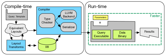
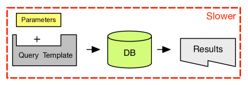
Figure 1. An overview of the Castor system (above) vs a traditional RDBMS (below).

Castor is an attempt to capture some of the optimization opportunities of static databases and to address the needs of these two scenarios. As Figure 1 illustrates, the input to Castor is a dataset and a parameterized query that a client will want to invoke on the data. The user then interacts with Castor using high-level commands to generate an efficient implementation of an in-memory datastore specialized for the dataset and the parameterized query. The commands available in Castor give the programmer tight control over the exact organization of the data in memory, allowing the user to trade off memory usage against query performance without the risk of introducing bugs. Castor also uses code generation techniques from high-performance in-memory databases to produce the low-level implementations required for efficient execution. The result is a package of data and code that uses significantly less memory than the most efficient in-memory databases and for some queries can even surpass the performance of in-memory databases that already rely on aggressive code generation and optimization (Neumann, 2011).

1.1. Contributions

Castor is made possible by three major technical contributions: a new notation to jointly represent the layout of the data in memory and the queries that will be computed on it, a set of deductive optimization rules that generalize traditional query optimization rules to jointly optimize the query and the data layout, and a type-driven layout compiler to produce both a binary representation of the data from the high-level data representation and specialized machine code for accessing it.

Integrated Layout & Query Language

We define the layout algebra, which extends the relational algebra (Codd, 1970) with layout operators that describe the particular data items to be stored and the layout of that data in memory. The layout algebra is flexible and can express many layouts, including row stores and clustered indexes. It supports nesting layouts, which gives control over data locality and supports prejoining of data. Our use of a language which combines query and layout operators makes it possible to write deductive transformations that change both the runtime query behavior and the data layout.

Deductive Optimization Rules

Castor provides a set of equivalence preserving transformations which can change both the query and the data layout. The user can apply these transformations to deductively optimize their query without worrying about introducing bugs. Alternatively, they can use Castor’s optimizer, which automatically selects a sequence of transformations. Castor’s specialized notation turns transformations that would be complex and global in other database systems into local syntactic changes.

Type-driven Layout Compiler

Existing relational synthesis tools use standard library data structures and make extensive use of pointer based data structures that hurt locality (Loncaric et al., 2018, 2016; Hawkins et al., 2011). Castor uses a specializing layout compiler that takes the properties of the data into account when serializing it. Before generating the layout, Castor generates an abstraction called a layout type which guides the layout specialization. For example, if the layout is a row-store with fixed-size tuples, the layout compiler will not emit a length field for the tuples. Instead, this length will be compiled directly into the query. This specialization process creates very compact datasets and avoids expensive branches in generated code.

High Performance Query Compiler

Castor uses code generation techniques from the high performance in-memory database literature (Neumann, 2011; Shaikhha et al., 2016; Tahboub et al., 2018; Rompf and Amin, 2015). It eschews the traditional iterator based query execution model (Graefe, 1994) in favor of a code generation technique that produces simple, easily optimized low-level code. Castor directly generates LLVM IR and augments the generated IR with information from the layout type that allows LLVM to further optimize it.

Empirical Evaluation

We empirically evaluate Castor on a benchmark derived from TPC-H, a standard database benchmark (Council, 2008). We show that Castor is competitive with the state of the art in-memory compiled database system Hyper (Neumann, 2011) while using significantly less memory. We also show that Castor scales to larger queries than the leading data-structure synthesis tool Cozy (Loncaric et al., 2018).

1.2. Limitations

Castor constructs read-only databases. This design decision limits the appropriate use cases for Castor but it enables important optimizations. Castor takes advantage of the absence of updates to tightly pack data together, which improves locality. Castor also aggressively specializes the compiled query by including information about the layout, such as lengths of arrays and offsets of layout structures. Providing this information to the compiler improves the generated code.

Only one parameterized query can be optimized at once. This is a limitation, but it is not a serious one. A multi-query workload can be supported by replicating the dataset and optimizing each query separately. Castor removes any data which is not needed by the query and it produces compact layouts for the data that remains. This reduces the overhead of the replication.

2. Motivating Example

We now describe the operation of Castor on an application from the software engineering literature. DemoMatch is a tool which helps users understand complex APIs using software demonstrations (Yessenov et al., 2017). DemoMatch maintains a database of program traces—computed offline—which it queries to discover how to use an API. DemoMatch is a good fit for Castor. The data in question is largely static: computing new traces is an infrequent task. The data is automatically queried by the tool, so there is no need to support ad-hoc queries. Finally, query performance is important for DemoMatch to work as an interactive tool.

2.1. Background

DemoMatch stores program traces as ordered collections of events (e.g., function calls). Traces have an inherent tree structure: each event has an enter and an exit and nested events may occur between the enter and exit.

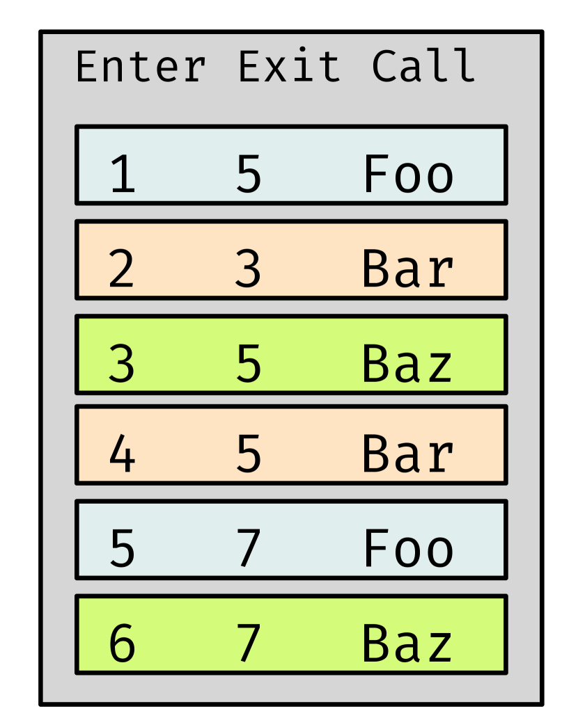
(a) In tabular form.

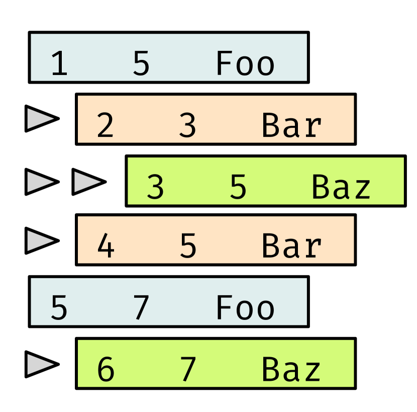
(b) In tree form.

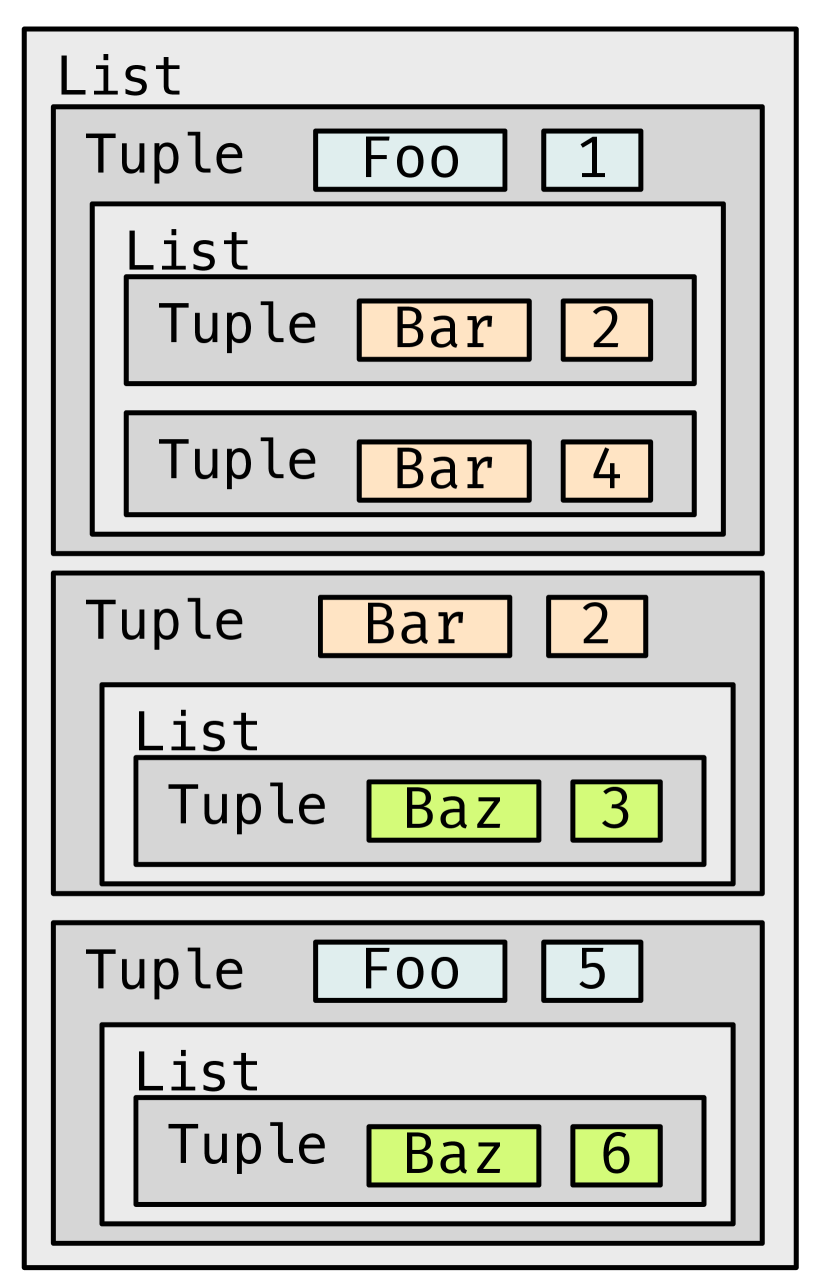
(c) As a nested layout.

Figure 2. Graphical representation of the DemoMatch data.

A critical query in the DemoMatch system finds nested calls to particular functions in a trace of program events:

$$\textsf{select}\ p.enter,\ c.enter\ \textsf{from}\ log\ \textsf{as}\ p,\ log\ \textsf{as}\ c\ \textsf{where}$$

$$\quad p.enter<c.enter\land c.enter<c.exit\land p.id=\$pid\land c.id=\$cid$$

We refer to the caller as the parent function and the callee as the child function. Let $p$ and $c$ be the traces of events inside the parent and child function bodies respectively. The join predicate $p.enter<c.enter\land c.enter<p.exit$ selects calls to the child function from inside the parent function. The predicate $p.id=\$pid\land c.id=\$cid$ selects the pair of functions that we are interested in, where $\$pid$ and $\$cid$ are parameters.

2.2. The Layout Algebra

Castor programs are written in a language called the layout algebra. The layout algebra is similar to the relational algebra, but as we will see shortly, it can represent the layout of data as well as the operation of queries. By design, it is more procedural than SQL, which is more akin to the relational calculus (Codd, 1971). For example, SQL leaves choices like join ordering to the query planner, whereas in the layout algebra join ordering is explicit.

In designing the layout algebra, we follow a well-worn path in deductive synthesis of creating a uniform representation that can capture all the refinement steps from a high-level program to a low-level one. Accordingly, the layout algebra can express programs which contain a mixture of high-level relational constructs and low-level layout constructs. At some point, a layout algebra program contains enough implementation information that the compiler can process it. We say that these programs are serializable (Sec. 3.3).

Here is the nested call query from Sec. 2.1 translated into the layout algebra:

$$\textsf{select}{}(\{enter_{p},enter_{c}\},\ \textsf{join}{}(enter_{p}<enter_{c}\land enter_{c}<exit_{p},$$

$$\quad\textsf{filter}{}(\$pid=id_{p},$$

$$\quad\quad\textsf{select}{}(\{id\mapsto id_{p},enter\mapsto enter_{p},exit\mapsto exit_{p}\},log)),$$

$$\quad\textsf{filter}{}(\$cid=id_{c},\textsf{select}{}(\{id\mapsto id_{c},enter\mapsto enter_{c}\},log))))$$

This program can be read as follows. filter takes a predicate as its first argument and a query as its second. It filters the query by the predicate. join takes a predicate as its first argument and queries as its second and third. The two queries are joined together using the predicate. select takes a list of expressions with optional names and a query, and selects the value of each expression for each tuple in the query, possibly renaming it.

The scoping rules for the layout algebra may look somewhat unusual, but they are intended to mimic the scoping conventions of SQL. In this query, the names $enter$, $exit$ and $id$ are field names in the $log$ relation. The select operators introduce new names for these fields, using the $\mapsto$ operator, so that $log$ can be joined with itself. We formalize the semantics of the layout algebra, including the scoping rules, in Sec. 3.2.

Note that at this point no layout is specified for $log$, so this is not a serializable program. Even though it is not serializable (and so cannot be compiled), this program still has well defined semantics. In Sections 2.4 to 2.6, we describe how layouts can be incrementally introduced by transforming the program until it is serializable.

2.3. Optimization Trade-offs

The nested call query is interesting because the data in question is fairly large—hundreds of thousands of rows—and keeping it fully in memory, or even better in cache, is a significant performance win. Therefore, minimizing the size of the data in memory should improve performance.

However, there is a fundamental trade-off between a more compact data representation and allowing for efficient access. Sometimes the two goals are aligned, but often they are not. For example, creating a hash index allows efficient access using a key, but introduces overhead in the form of a mapping between hash keys and values.

In the rest of this section we examine three layouts at different points in this trade-off space: a compact nested layout with no index structures (Figure 4(a)), a layout based on a single hash index (Figure 4(b)), and a layout based on a hash index and an ordered index (Figure 4(c)). A priori, none of these layouts is clearly superior. The hash based layout is the largest, but has the best lookup properties. The nested layout precomputes the join and uses nesting to reduce the result size, but is more expensive for lookups. The last layout must compute the join at runtime but it has indexes that will make that computation fast. The power of Castor is that it allows users to effectively explore different layout trade-offs by freeing them from the necessity to ensure the correctness of each candidate.

2.4. Nested Layout

Our first approach to optimizing the nested call query is to materialize the join, since joins are usually expensive, and to use nesting to reduce the size of the resulting layout.

The first step is to apply transformation rules (Sec. 4.2) to hoist and merge the filters. Now the join is in a term with no query parameters, so it can be evaluated at compile time:

$$\textsf{select}{}(\{enter_{p},enter_{c}\},\ \textsf{filter}{}(\$pid=id_{p}\land\$cid=id_{c},$$

$$\quad\textsf{join}{}(enter_{p}<enter_{c}\land enter_{c}<exit_{p},$$

$$\quad\quad\textsf{select}{}(\{id\mapsto id_{p},enter\mapsto enter_{p},exit\mapsto exit_{p}\},log),$$

$$\quad\quad\textsf{select}{}(\{id\mapsto id_{c},enter\mapsto enter_{c}\},log))))$$

After applying two more rules—projection to eliminate unnecessary fields (Sec. 4.3) and join elimination (Sec. 4.6)—the result is the layout expression represented in code in Figure 3 and graphically in Figure 4(a). In this program we see our first layout operators: $\textsf{{list}}{}(\cdot,\cdot)$ and $\textsf{{tuple}}_{\textsf{cross}}([\dots])$. The layout algebra extends the relational algebra with these operators, allowing us to write layout expressions, which describe how their arguments will be laid out in memory.

$$\textsf{select}{}(\{enter_{p},enter_{c}\},\ \textsf{filter}{}(id_{c}=\$cid\land id_{p}=\$pid,$$

$$\quad\textsf{{list}}{}(\textsf{select}{}(\{id\mapsto id_{p},enter\mapsto enter_{p},exit\mapsto exit_{p}\},log)\ \textsf{as}\ lp,$$

$$\quad\quad\textsf{{tuple}}_{\textsf{cross}}([\textsf{{scalar}}(lp.id_{p}),\textsf{{scalar}}(lp.enter_{p}),$$

$$\quad\quad\quad\textsf{{list}}{}(\textsf{filter}{}(lp.enter_{p}<enter_{c}\land enter_{c}<lp.exit_{p},$$

$$\quad\quad\quad\quad\textsf{select}{}(\{id\mapsto id_{c},enter\mapsto enter_{c}\},log))\ \textsf{as}\ lc,$$

$$\quad\quad\quad\quad\textsf{{tuple}}_{\textsf{cross}}([\textsf{{scalar}}(lc.id_{c}),\textsf{{scalar}}(lc.enter_{c})]))]))))$$

Figure 3. Nested list layout.

Figure 3 can be read as follows. The operator $\textsf{{list}}{}(log\ \textsf{as}\ l,q)$ creates a list with one element for every tuple in $log$. Each element in the list is laid out according to $q$. For example, the outermost list in Figure 3 creates a list from the $id$, $enter$ and $exit$ fields of the $log$ relation. Each row in the list is laid out as a $\textsf{{tuple}}_{\textsf{cross}}$. The first two elements in the tuple are the scalar representations of the $id_{p}$ and $enter_{p}$ fields, and the third element is a nested list. Note that the content of that inner list is filtered based on the value of $lp.enter_{p}$ and $lp.exit_{p}$, and each element laid out as just a pair of two scalars $id_{c}$ and $enter_{c}$.

The query is now serializable because it satisfies a set of rules described in Sec. 3.3. At a high-level, the rules require that we never use a relation without specifying its layout, a requirement that in this case is satisfied because all references to the original log relation appear in the first arguments of list operators.

Figure 4(a) shows the structure of the resulting layout. This layout is quite compact. It is smaller than the fully materialized join because of the nesting; the caller id and enter fields are only stored once for each matching callee record. When we benchmark this query, we find found that it performs reasonably well (11.5ms) and is fairly small (50Mb).

We can make this layout more compact by applying further transformations. For example, we know that $enter_{p}<enter_{c}<exit_{p}$. If we store $enter_{c}-enter_{p}$ instead of $enter_{c}$ we can save some space by using fewer bits. The ability to take advantage of this kind of knowledge about the structure of the data is an important feature of our approach.

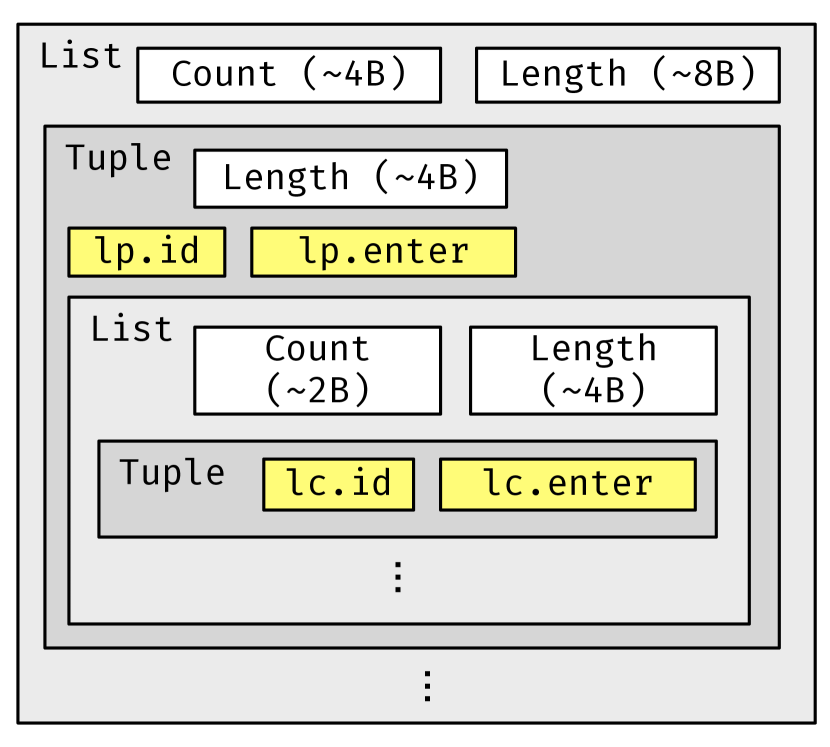
(a) Nested.

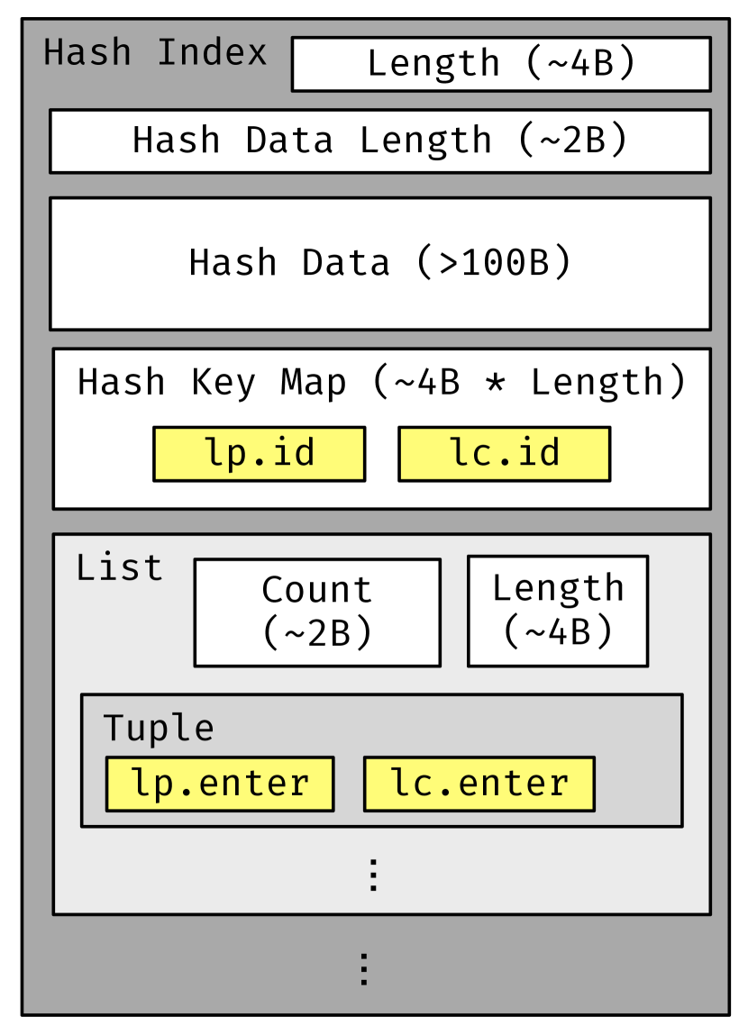
(b) Hash-index.

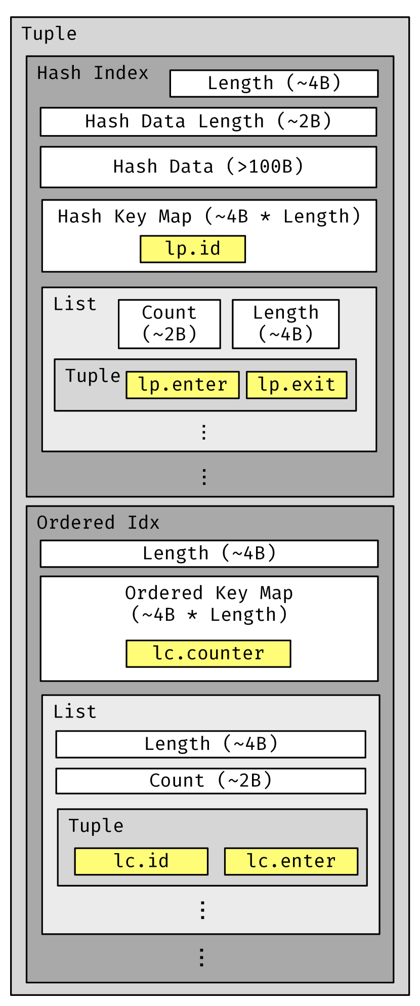
(c) Ordered-index.

Figure 4. Sample layouts (relational data is highlighted).

2.5. Hash-index Layout

Now we optimize for lookup performance by fully materializing the join and creating a hash index. This layout will be larger than the nested layout but look ups into the hash index will be quick, which will make evaluating the equality predicates on $id$ fast. Figure 4(b) shows the structure of the resulting layout. When we evaluate the query, we find that it is much faster (0.4ms) but is larger than the nested query (60Mb).

2.6. Hash- and Ordered-index Layout

Finally, we investigate a layout which avoids the full join materialization, but still has enough indexing to be fast. We can see that the join condition is a range predicate, so we would like to use an index that supports efficient range queries to make that predicate efficient (Sec. 4.5). Then we can push the filters and introduce a hash table to select $id_{p}$. The resulting layout is shown in Figure 4(c). This layout will be larger than the original relation, but smaller than the other two layouts (9.8Mb), and it allows for much faster computation of the join and one of the filters (0.6ms).

This program introduces three new operators: ordered-idx, hash-idx and depjoin. ordered-idx creates indexes that support efficient range queries. Its first argument defines the set of keys and its second argument defines the values and their layout as a function of the keys. The remaining arguments are the upper and lower bounds to use when reading the index ($p.enter_{p}$ and $p.exit$ in this case). hash-idx is similar, but it creates efficient point indexes (in this query, $\$pid$ is the key).

$$\textsf{select}{}(\{enter_{p},enter_{c}\},\ \textsf{depjoin}{}(\textsf{{hash-idx}}{}(\textsf{select}{}(\{id\},\ log)\ \textsf{as}\ h,$$

$$\quad\textsf{{list}}{}(\textsf{filter}{}(h.id=id\land enter>exit,\ log)\ \textsf{as}\ lh,$$

$$\quad\quad\textsf{{tuple}}_{\textsf{cross}}([\textsf{{scalar}}(lh.enter\mapsto enter_{p}),\ \textsf{{scalar}}(lh.exit)])),$$

$$\quad\$pid)\ \textsf{as}\ p,$$

$$\quad\textsf{filter}{}(id=\$cid,\ \textsf{{order\-ed-idx}}{}(\textsf{select}{}(\{enter\},log)\ \textsf{as}\ o,$$

$$\quad\quad\textsf{{list}}{}(\textsf{filter}{}(enter=o.enter,\ log)\ \textsf{as}\ lo,$$

$$\quad\quad\quad\textsf{{tuple}}_{\textsf{cross}}([\textsf{{scalar}}(lo.id),\ \textsf{{scalar}}(lo.enter\mapsto enter_{c})])),$$

$$\quad\quad p.enter_{p},\ p.exit))))$$

The more interesting operator is depjoin, which implements a dependent join. A dependent join is one where the right-hand-side of the join can refer to fields from the left-hand-side. In the depjoin operator, the left-hand-side is given a name (here it is $p$) that the right-hand-side can use to refer to its fields. One way to think about a dependent join is as a relational for loop: it evaluates the right-hand-side for each tuple in the left-hand-side, concatenating the results. Unlike the layout operators list, hash-idx and ordered-idx, depjoin executes entirely at runtime. It does not introduce any layout structure.

3. Language

In this section we describe the layout algebra in detail. The layout algebra starts with the relational algebra and extends it with layout operators. These layout operators have relational semantics, but they also have layout semantics which describes how to serialize them to data structures. The combination of relational and layout operators allows the layout algebra to express both a query and the data store that supports the execution of the query.

Programs in the layout algebra have three semantic interpretations:

1. The relational semantics describes the behavior of a layout algebra program at a high level. We define this semantics using a theory of ordered finite relations (Cheung et al., 2013). According to this semantics, A layout algebra program can be evaluated to a relation in a context containing relations and query parameters.

2. The layout semantics describes how the compiler creates a data file from a serializable layout algebra program. The layout semantics operates in a context which contains relations, but not query parameters.

3. The runtime semantics describes how the compiled query executes, reading the layout file and using the query parameters to produce the query output. The runtime semantics operates in a context which contains query parameters but not relations.

These three semantics are connected: the layout semantics and the runtime semantics combine to implement the relational semantics. The relational semantics serves as a specification. An interpreter written according to the relational semantics should execute layout algebra programs in the same way as our compiler. In this section, we discuss the relational semantics in detail. We leave the detailed discussion of the layout and runtime semantics to Appendix A and Appendix B.

3.1. Syntax

$$x ::= \ \text{identifiers}\quad o::=\textsf{asc}~{}|~{}\textsf{desc}\quad\tau::=\textsf{cross}~{}|~{}\textsf{concat}$$

$$v ::= \ \text{integers}~{}|~{}\text{strings}~{}|~{}\text{Booleans}~{}|~{}\text{floats}~{}|~{}\text{dates}~{}|~{}\textsf{null}$$

$$e ::= \ v~{}|~{}x~{}|~{}e+e^{\prime}~{}|~{}e-e^{\prime}~{}|~{}e\times e^{\prime}~{}|~{}e/e^{\prime}~{}|~{}e\ \%\ e^{\prime}~{}|~{}e<e^{\prime}~{}|~{}e\leq e^{\prime}~{}|~{}e>e^{\prime}$$

— $$\ e\geq e^{\prime}~{}|~{}e=e^{\prime}~{}|~{}\textsf{if}\ e\ \textsf{then}\ e_{t}\ \textsf{else}\ e_{f}~{}|~{}\textsf{exists}(q)~{}|~{}\textsf{first}(q)~{}|~{}\textsf{count}()$$

— $$\ \textsf{sum}(e)~{}|~{}\textsf{min}(e)~{}|~{}\textsf{max}(e)~{}|~{}\textsf{avg}(e)$$

$$t ::= \ \{x_{1}\mapsto e_{1},\dots,x_{k}\mapsto e_{k}\}$$

$$q ::= \ \textsf{relation}(x)~{}|~{}\textsf{dedup}(q)~{}|~{}\textsf{select}(t,q)~{}|~{}\textsf{filter}(e,q)~{}|~{}\textsf{join}(e,q,q^{\prime})$$

— $$\ \textsf{group-by}(t,[x_{1},\dots,x_{m}],q)~{}|~{}\textsf{order-by}([e_{1}\ o_{1},\dots,e_{m}\ o_{m}],q)$$

— $$\ \textsf{depjoin}(q\ \textsf{as}\ x,q^{\prime})~{}|~{}\textsf{{scalar}}(x\mapsto e)~{}|~{}\textsf{{tuple}}_{\tau}(t)~{}|~{}\textsf{{list}}{}(q_{r}\ \textsf{as}\ x,q)$$

— $$\ \textsf{{hash-idx}}{}(q_{k}\ \textsf{as}\ x,q_{v},t_{k})~{}|~{}\textsf{{order\-ed-idx}}{}(q_{k}\ \textsf{as}\ x,q_{v},t_{lo},t_{hi})~{}|~{}\emptyset$$

Figure 5. Syntax of the layout algebra.

Figure 5 shows the syntax of the layout algebra. Note that the layout algebra can be divided into relational operators (select, filter, join, etc.) and layout operators (list, hash-idx, etc.). The layout algebra is a strict superset of the relational algebra. In fact, the layout operators have relational semantics in addition to byte-level data layout semantics (see Sec. 3.2.2).

3.2. Semantics

$$Id=(Scope?,Name)\quad Context=Tuple=\{Id\mapsto Value\}$$

$$Relation=[Tuple]$$

$$\sigma:Context\enspace\delta:Id\mapsto Relation\enspace s:Id\enspace t:Tuple\enspace v:Value\enspace r:Relation$$

(1) $$\inference{\forall n.\ n\not\in\sigma\lor n\not\in\sigma^{\prime}}{\sigma\cup\sigma^{\prime}=\{n_{i}\mapsto v_{i}~{}|~{}\sigma[n_{i}]=v_{i}\lor\sigma^{\prime}[n_{i}]=v_{i}\}}$$

(2) $$\inference{t=\{n_{1}\mapsto e_{1},\dots,n_{m}\mapsto e_{m}\}&\forall i.\ \sigma,\delta|-e_{i}\Downarrow v_{i}}{\sigma,\delta|-t\Downarrow\{n_{1}\mapsto v_{1},\dots,n_{m}\mapsto v_{m}\}}$$

(3) $$\inference{\delta[n]=r}{\sigma,\delta|-\textsf{relation}(n)\Downarrow r}$$

(4) $$\inference{\sigma,\delta|-q\Downarrow r_{q}\\ r=[t~{}|~{}t<-r_{q}\quad\sigma\cup t,\delta|-e\Downarrow\textsf{true}]}{\sigma,\delta|-\textsf{filter}(e,q)\Downarrow r}$$

(5) $$\inference{\sigma,\delta|-q\Downarrow r&r^{\prime\prime}=\left[t^{\prime}~{}\Big{|}~{}{\begin{array}[]{c}t<-r,\ t^{\prime}<-r^{\prime}\quad\sigma\cup t_{s},\delta|-q^{\prime}\Downarrow r^{\prime}\\ t_{s}=\{s.f\mapsto v~{}|~{}(f\mapsto v)\in t\}\end{array}}\right]}{\sigma,\delta|-\textsf{depjoin}(q\ \textsf{as}\ s,q^{\prime})\Downarrow r^{\prime\prime}}$$

(6) $$\inference{\sigma,\delta|-e\Downarrow v}{\sigma,\delta|-\textsf{{scalar}}(n\mapsto e)\Downarrow[\{n\mapsto v\}]}$$

(7) $$\inference{}{\sigma,\delta|-\emptyset\Downarrow[\ ]}$$

(8) $$\inference{\sigma,\delta|-\textsf{depjoin}(q_{r}\ \textsf{as}\ s,q)\Downarrow r}{\sigma,\delta|-\textsf{{list}}{}(q_{r}\ \textsf{as}\ s,q)\Downarrow r}$$

(9) $$\inference{}{\sigma,\delta|-\textsf{{tuple}}_{\tau}([~{}])\Downarrow[~{}]}$$

(10) $$\inference{\sigma,\delta|-q_{1}\Downarrow r_{q}&\sigma,\delta|-\textsf{{tuple}}_{\tau}([q_{2},\dots,q_{n}])\Downarrow r_{qs}}{\sigma,\delta|-\textsf{{tuple}}_{\textsf{cross}}([q_{1},\dots,q_{n}])\Downarrow[t\cup ts~{}|~{}t<-r_{q},ts<-r_{qs}]}$$

(11) $$\inference{\sigma,\delta|-\textsf{depjoin}(q_{k}\ \textsf{as}\ s,\textsf{filter}{}(l_{lo}\leq s.x\leq l_{hi},q_{v}))\Downarrow r\\ \textsc{schema}(q_{k})=[x]}{\sigma,\delta|-\textsf{{order\-ed-idx}}{}(q_{k}\ \textsf{as}\ s,q_{v},l_{lo},l_{hi})\Downarrow r}$$

Figure 6. Selected relational semantics of the layout algebra.

The semantics (Figure 6) operates on three kinds of values: scalars, tuples and relations. Scalars are values like integers, Booleans, and strings. Tuples are finite mappings from field names to scalar values. Relations are represented as finite, ordered sequences of tuples. $[~{}]$ stands for the empty relation, $:$ is the relation constructor, and $\mathbin{+\!\!+}$ denotes the concatenation of relations.

We use sequences instead of sets for two reasons. First, sequences are more like bag semantics than the set semantics of the original relational algebra. This choice brings the layout algebra more in line with the semantics of SQL, which is convenient for our implementation. Second, sequences allow us to represent query outputs which have an ordering.

In the semantic rules, $\sigma$ is an evaluation context; it maps names to scalar values. $\delta$ is a relational context; it maps names to relations. We separate the two contexts because the relational context $\delta$ is global and immutable; it consists of a universe of relations that exist when the query is executed (or compiled) which are contained in some other database system. The evaluation context $\sigma$ initially contains the query parameters, but some operators introduce new bindings in $\sigma$. $\cup$ denotes the binding of a tuple into an evaluation context. Read $\sigma\cup t$ as a new evaluation context that contains the fields in $t$ in addition to the names already in $\sigma$.

In the rules, $|-$ separates contexts and expressions and $\Downarrow$ separates expressions and results. Read $\sigma,\delta|-l\Downarrow s$ as “the layout $l$ evaluates to the relation $s$ in the context $\sigma,\delta$.”

We borrow the syntax of list comprehensions to describe the semantics of the layout algebra operators. For example, consider the list comprehension in the filter rule: $[t~{}|~{}t<-r_{q},(\sigma\cup t,\delta|-e\Downarrow\textsf{true})]$, which corresponds to the expression $\textsf{filter}(e,q)$. This list comprehension filters $r_{q}$ by the predicate $e$ where $r_{q}$ is the relation produced by $q$. $e$ is evaluated in a context $\sigma\cup t$ for each tuple $t$ in $r_{q}$.

Comprehensions that contain multiple $<-$, as in the join rule, should be read as a cross product.

3.2.1. Relational Operators

First, we describe the semantics of the relational operators: relation, filter, join, select, group-by, orderby, dedup, and depjoin. These operators are modeled after their equivalent SQL constructs. For brevity and because they are straightforward, we omit the rules for selection with aggregates, group-by, and order-by from Figure 6.

relation returns the contents of a relation in the relational context $\delta$. filter filters a relation by a predicate $e$. join takes the cross product of two relations and filters it using a predicate $e$.

select is used for projection, aggregation, and renaming fields. It takes a tuple expression $t$ and a relation $r$. If $t$ contains no aggregation operators, then a new tuple will be constructed according to $t$ for each tuple in $r$. If $t$ contains an aggregation operator (count, sum, min, max, avg), then select will aggregate the rows in $r$. If $t$ contains both aggregation and non-aggregation operators, then the non-aggregation operators will be evaluated on the last tuple in $r$.

group-by takes a list of expressions, a list of fields, and a relation. It groups the tuples in the relation by the values of the fields, then computes the aggregates in the expression list. order-by takes a list of expression-order pairs and a relation. It orders the tuples in the relation using the list of expressions to compute a key. dedup removes duplicate tuples.

Finally, depjoin denotes a dependent join, where the right-hand-side of the join can depend on values from the left-hand-side. It is similar to a for-each loop; $\textsf{depjoin}(q\ \textsf{as}\ n,\ q^{\prime})$ can be read “evaluate $q^{\prime}$ for each tuple in $q$ and concatenate the results.” We use depjoin as a building block to define the semantics of the layout operators.

3.2.2. Layout Operators

We extend the relational algebra with layout operators that specify the layout of data in memory at a byte level. The nesting and ordering of the layout operators correspond to the nesting and ordering of the data structures that they represent. Nesting allows data that is accessed together to be stored together, increasing spatial locality. Note that layout operators can capture the results of executing common relational algebra operations such as joins or selections, allowing query processing to be performed at compile time. In addition, layout primitives can express common relational data storage patterns, such as row stores and clustered indexes.

Castor supports the following data structures:

Scalars: Scalars can be machine integers (up to 64 bits), strings, Booleans, and decimal fixed-point.

Tuples: Tuples are layouts that can contain layouts with different types. If a collection contains tuples, all the tuples must have the same number of elements and their elements must have compatible types. Tuples can be read either by taking the cross product or concatenating their sub-layouts.

Lists: Lists are variable-length layouts. Their contents must be of the same type.

Hash indexes: Hash indexes are mappings between scalar keys and layouts, stored as hash tables. Like lists, their keys must have the same type.

Ordered indexes: Ordered indexes are mappings between scalar keys and layouts, stored as ordered mappings.

Each data structure has a corresponding layout operator. The layout operators are the novel part of the layout algebra and their semantics are therefore non-standard. The relational semantics of the layout operators are in Figure 6. Although the layout operators can be used to construct complex, nested layouts, they evaluate to flat relations of tuples of scalars, just like the relational operators. The rules in Figure 6 only describe the relational behavior of the layout operators; they do not address the question of how data is laid out or how it is accessed. We discuss these aspects of the layout operators in Appendix A.

The simplest layout operators are scalar and tuple. The scalar represents a single scalar value. Evaluating a scalar operator produces a relation containing a single tuple. The tuple operator represents a fixed-size, heterogeneous list of layouts. When evaluated, each layout in the tuple produces a relation, which are combined either with a cross product or by concatenation.

Note that evaluating a tuple operator produces a relation not a tuple. Although these semantics are slightly surprising, there are two reasons why we chose this behavior. First, it is consistent with the other layout operators, all of which evaluate to relations. Second, tuples can contain other layouts (lists for example) which themselves evaluate to relations.

The remaining layout operators—list, hash-idx and ordered-idx—have a similar structure. We discuss the list operator in detail. Equation 8 specifies the behavior of list. Note that list is essentially an alias for depjoin. Like depjoin, list takes two arguments: $q_{r}$ and $q$. These two arguments should be interpreted as follows: $q_{r}$ describes the data in the list. Each element of the list has a corresponding tuple in $q_{r}$, so the length of the list is the same as the length of $q_{r}$. One can think of each tuple in $q_{r}$ as a kind of key that determines the contents of each list element. On the other hand, $q$ describes how each list element is laid out. $q$ will be evaluated separately for each tuple in $q_{r}$. It determines for each “key” in $q_{r}$, what the physical layout of each list element will be, as well as how that element must be read.

Returning to the query in Sec. 2.4, the inner list operator

$$\textsf{{list}}{}(\textsf{filter}{}(lp.enter_{p}<enter_{c}\land enter_{c}<lp.exit_{p},$$

$$\quad\textsf{select}{}(\{id\mapsto id_{c},\ enter\mapsto enter_{c}\},\ log))\ \textsf{as}\ lc,$$

$$\quad\quad\textsf{{tuple}}_{\textsf{cross}}([\textsf{{scalar}}(lc.id_{c}),\ \textsf{{scalar}}(lc.enter_{c})]))$$

selects the tuples in $log$ where $enter_{c}$ is between $enter_{p}$ and $exit_{p}$, and creates a list of these tuples. The first argument describes the contents of the list and the second describes their layout. This program will generate a layout that has a list of tuples, structured as $[(id_{c1},enter_{c1}),\dots,(id_{cn},enter_{cn})]$.

hash-idx and ordered-idx are similar to list. They have a query $q_{k}$ that describes which keys are in the index and a query $q_{v}$ that describes the contents and layout of the values in the index. For example, in:

$$\textsf{{hash-idx}}{}(\textsf{select}{}(\{id\},log)\ \textsf{as}\ h,\ \textsf{{list}}{}(\textsf{filter}{}(\{id=h.id\},log)\ \textsf{as}\ l,$$

$$\quad\textsf{{tuple}}_{\textsf{cross}}([\textsf{{scalar}}(l.enter),\textsf{{scalar}}(l.exit)])),\ \$pid),$$

the keys to the hash-index are the $id$ fields from the $log$ relation. For each of these fields, the index contains a list of corresponding $(enter,exit)$ pairs, stored in a tuple. When the hash-index is accessed, $\$pid$ is used as the key. This program generates a layout of the form: $\{id\mapsto[(enter,exit),\dots],\dots\}$, which is a hash-index with scalars for keys and lists of tuples for values.

3.2.3. Scopes & Name Binding

The scoping rules of the layout algebra are somewhat more complex than the relational algebra. There are two ways to bind a name in the layout algebra: by creating a relation or by using an operator which creates a scope.

All of the operators in the layout algebra return a relation. Some operators simply pass through the names in their parameter relations. Others, such as select and scalar can be used for renaming or for creating new fields.

Some operators, such as depjoin, create a scope. A scope is a tag which uniquely identifies the binding site of a name. For example, in $\textsf{depjoin}{}(q\ \textsf{as}\ s,q^{\prime})$, a field $f$ from $q$ is bound in $q^{\prime}$ as $s.f$. Scoped names with distinct scopes are distinct and scoped names are distinct from unscoped names. We add scopes to the layout algebra as a syntactically lightweight mechanism for renaming an entire relation. Renaming entire relations is necessary because shadowing is prohibited in the layout algebra. Prohibiting shadowing removes a major source of complexity when writing transformations. While we could use select for renaming, we opted to add scopes so that renaming at binding sites would be part of the language rather than a pervasive and verbose pattern.

There are still situations when renaming entire relations using select is necessary. For example, in a self-join one side of the join must be renamed.

3.3. Staging & Serializability

Another way to view the three semantic interpretations is from the point of view of multi-stage programming. A serializable layout algebra program can be evaluated in two stages: the layout is constructed in a compile-time stage, then the compiled query reads the layout and processes it in a run-time stage. However, while traditionally program staging is used to implement code specialization, in the layout algebra staging is used to implement data specialization. This difference in focus leads to different implementation challenges. In particular, the “unstaged” version of a layout algebra program is often large (tens to hundreds of megabytes). The layout algebra compiler must be carefully designed to handle this scale.

In Sec. 3.2.2, we explained how the layout operators execute in two stages: one stage at compile time and one stage at query runtime. Only a subset of layout algebra programs can be separated in this way. We say that programs which can be properly staged are serializable.

A program is serializable if and only if the names referred to in compile (resp. run) time contexts are bound in compile (resp. run) time contexts. An expression is in a compile-time context if it appears in the first argument to list, hash-idx, ordered-idx, or scalar. Otherwise, it is in a run-time context. We consider the relations in $\delta$ to be bound in a compile-time context and query parameters to be bound in a run-time context. The compiler uses a simple type system that tracks the stage of each name in the program to check for serializability.

Transforming a program into a serializable form is a key goal of our automatic optimizer (Sec. 6). Many of the rules that the optimizer applies can be seen as moving parts of the query between stages.

4. Transformations

In this section, we define semantics preserving transformation rules that optimize query and layout performance. These rules change the behavior of the program with respect to the layout and runtime semantics while preserving it with respect to the relational semantics. These rules subsume standard query optimizations because in addition to changing the structure of the query, they can also change the structure of the data that the query processes.

4.1. Notation

Transformations are written as inference rules. When writing inference rules, $e$ will refer to scalar expressions and $q$ will refer to layout algebra expressions. $E$ and $Q$ will refer to lists of expressions and layouts. In general, the names we use correspond to those used in the syntax description (Figure 5). If we need to refer to a piece of concrete syntax, it will be formatted as e.g., concat or x.

To avoid writing many trivial inductive rules, we define contexts. The definition is straightforward, so we leave it to the appendix (Figure 11). If $C$ is a context and $q$ is a layout algebra expression, then $C[q]$ is the expression obtained by substituting $q$ into the hole in $C$. In addition to contexts, we define two operators: $\xrightarrow{t}{}$ and $->$. $q\xrightarrow{t}{}q^{\prime}$ means that the layout algebra expression $q$ can be transformed into $q^{\prime}$ and $q->q^{\prime}$ means that $q$ can be transformed into $q^{\prime}$ in any context. The relationship between these two operators is:

$$q->q^{\prime}\equiv\forall C.\ C[q]\xrightarrow{t}{}C[q^{\prime}]$$

4.2. Relational Optimization

There is a broad class of query transformations that have been developed in the query optimization literature (Jarke and Koch, 1984; Chaudhuri, 1998). These transformations can generally be applied directly in Castor, at least to the relational operators. For example, commuting and reassociating joins, filter pushing and hoisting, and splitting and merging filter and join predicates are implemented in Castor. Although producing optimal relational algebra implementations of a query is explicitly a non-goal of Castor, these kinds of transformations are important for exposing layout optimizations.

4.3. Projection

Projection, or the removal of unnecessary fields from a query, is an important transformation because many queries only use a small number of fields; the most impactful layout specialization that can be performed for these queries is to remove unneeded fields.

First, we need to decide what fields are necessary. For a query $q$ in some context $C$, the necessary fields in $q$ are visible in the output of $C[q]$ or are referred to in $C$. Let $\textsc{schema}(\cdot)$ be a function from a layout $q$ to the set of field names in the output of $q$. Let $\textsc{names}(\cdot)$ be a function which returns the set of names in a context or layout expression. Let $\textsc{needed}(\cdot,\cdot)$ be a function from contexts $C$ and layouts $q$ to the set of necessary fields in the output of $q$:

$$\textsc{needed}(C,q)=\textsc{schema}(q)\cap(\textsc{schema}(C[q])\cup\textsc{names}(C))$$

$\textsc{needed}(\cdot,\cdot)$ can be used to define transformations which remove unnecessary parts of a layout. For example, this rule removes unnecessary fields from tuples:

$$\inference{Q^{\prime}=[q~{}|~{}q\in Q,\textsc{needed}(C,q)\neq\emptyset]}{C[\textsf{{tuple}}(Q)]\xrightarrow{t}{}C[\textsf{{tuple}}(Q^{\prime})]}$$

There is a similar rule for select and groupby operators.

The projection rules differ from the others in this section because they refer to the context $C$. The other rules can be applied in any context. The context is important for the projection rules because without it, all the fields in a layout would be visible and therefore “necessary”. Referring to the context allows us to determine which fields are visible to the user.

4.4. Precomputation

A simple transformation that can improve query performance is to compute and store the values of parameter-free terms. This transformation is similar to partial evaluation. The following rule precomputes a static layout algebra expression:

$$\inference{\textsc{schema}(\boxed{q})=[f_{1},\dots,f_{k}]&x\ \text{is fresh}}{\boxed{q}->\textsf{{list}}{}(\boxed{q}\ \textsf{as}\ x,\textsf{{tuple}}_{\textsf{cross}}([\textsf{{scalar}}(x.f_{1}),\dots,\textsf{{scalar}}(x.f_{k})]))}$$

Hoisting static expressions out of predicates can also be very profitable:

$$\inference{x,y\ \text{are fresh}\quad\boxed{e^{\prime}}\ \text{is a term in}\ e\quad\textsc{names}(e^{\prime})\cap\textsc{schema}(q)=\emptyset}{\textsf{filter}{}(e,q)->\textsf{depjoin}(\textsf{{scalar}}(e^{\prime}\mapsto y)\ \textsf{as}\ x,\textsf{filter}{}(e[e^{\prime}:=x.y],q))}.$$

If the expression $e^{\prime}$ can be precomputed and stored instead of being recomputed for every invocation of the filter. Similar transformations can be applied to any operator that contains an expression. This rule is useful when the filter appears inside a layout operator. For example, in $\textsf{{list}}{}(q\ \textsf{as}\ x,\textsf{filter}(e,q^{\prime}))$, an expression $e^{\prime}$ can be hoisted out of the filter if it refers to the fields in $q$ but not if it refers to the fields in $q^{\prime}$.

In a similar vein, select operators can be partially precomputed. For example:

$$\inference{y^{\prime}\ \text{is fresh}&q_{v}^{\prime}=\textsf{select}{}(\{\textsf{sum}(e)\mapsto y^{\prime}\},q_{v})}{\begin{aligned} &\textsf{select}{}(\{\textsf{sum}(e)\mapsto y\},\textsf{{order\-ed-idx}}{}(q_{k}\ \textsf{as}\ x,q_{v},t_{lo},t_{hi}))->\\ &\quad\textsf{select}{}(\{\textsf{sum}(y^{\prime})\mapsto y\},\textsf{{order\-ed-idx}}{}(q_{k}\ \textsf{as}\ x,q_{v}^{\prime},t_{lo},t_{hi}))\end{aligned}}.$$

After this transformation, the ordered index will contain partial sums which will be aggregated by the outer select. This rule is particularly useful when implementing grouping and filtering queries, because the filter can be replaced by an index and the aggregate applied to the contents of the index. A similar rule also applies to select and list. A simple version of this rule applies to hash-idx; in that case, the outer select is unnecessary.

This transformation is combined with group-by elimination (Sec. 4.5) in TPC-H query 1 to construct a layout that precomputes most of the aggregation.

4.5. Partitioning

Partitioning is a fundamental layout transformation that splits one layout into many layouts based on the value of a field or expression. A partition of a relation $r$ is defined by an expression $e$ over the fields in $r$. Tuples in $r$ are in the same partition if and only if evaluating $e$ over their fields gives the same value.

Let $\textsc{part}(\cdot,\cdot,\cdot)$ be a function which takes a layout $q$, a partition expression $e$, and a name $x$, and returns a query for the partition keys and a query for the partitions:

$$\textsc{part}(q,\boxed{e},x)=(\textsf{dedup}(\textsf{select}(\boxed{e},q)),\ \textsf{filter}(x.e=\boxed{e},q)).$$

In this definition, $q_{k}$ evaluates to the unique valuations of $e$ in $r$. These are the partition keys. Note that the expression $q_{v}$ contains a free scope $x$. We use $x.e$ to denote the expression $e$ with its names qualified by the scope $x$. Once $x.e$ is bound to a particular partition key, $q_{v}$ evaluates to a relation containing only tuples in that partition.

The partition function is used to define rules that create hash indexes and ordered indexes from filters:

$$\inference{x,n\ \text{is fresh}&\textsc{part}(q,\boxed{e},x)=(q_{k},q_{v})}{\textsf{filter}(\boxed{e}=e^{\prime},q)->\textsf{{hash-idx}}{}(q_{k}\ \textsf{as}\ x,q_{k},q_{v},e^{\prime})},$$

$$\inference{x\ \text{is fresh}&\textsc{part}(q,\boxed{e},x)=(q_{k},q_{v})}{\textsf{filter}(e_{l}\leq\boxed{e}\land\boxed{e}\leq e_{h},q)->\textsf{{order\-ed-idx}}{}(q_{k}\ \textsf{as}\ x,q_{k},q_{v},e_{l},e_{h})}.$$

Partitioning also leads immediately to a rule that eliminates $\textsf{group-by}{}(\cdot)$:

$$\inference{x\ \text{is fresh}&\textsc{part}(q,\boxed{K},x)=(q_{k},q_{v})}{\textsf{group-by}{}(\boxed{K},E,q)->\textsf{{list}}{}(q_{k}\ \textsf{as}\ x,\textsf{select}{}(E,q_{v}))}.$$

There is a slight abuse of notation in this rule. $K$ is a list of expressions, so the filter in $q_{v}$ must have an equality check for each expression in $K$. This group-by elimination rule is used in many of the TPC-H queries which contain group-bys.

4.6. Join Elimination

Castor’s layout operators admit several options for join materialization. Since joins are often the most expensive operations in a relational query, choosing a good join materialization strategy is critical. Castor does not suggest a join strategy but it provides the necessary tools for an expert user.

Partitioning can be used to implement join materialization: a powerful transformation that can significantly reduce the computation required to run a query, at the cost of increasing the size of the data that the query runs on. Our layout language allows for several join materialization strategies.

For example, joins can be materialized as a list of pairs:

$$\inference{x\ \text{is fresh}\quad\textsc{part}(q,\boxed{e},x)=(q_{k},q_{v})\quad\textsc{part}(q^{\prime},\boxed{e^{\prime}},x)=(\cdot,q_{v}^{\prime})}{\textsf{join}(\boxed{e}=\boxed{e^{\prime}},q,q^{\prime})->\textsf{{list}}{}(q_{k}\ \textsf{as}\ x,\textsf{{tuple}}_{\textsf{cross}}([q_{v},q_{v}^{\prime}]))}.$$

Each pair in this layout contains the tuples that should join together from the left- and right-hand-sides of the join.

Joins can also be materialized as nested lists:

$$\inference{x\ \text{is fresh}\enspace\textsc{schema}(q)=[f_{1},\dots,f_{n}]\enspace F=\textsf{{scalar}}(f_{1}),\dots,\textsf{{scalar}}(f_{n})}{\textsf{join}(e=e^{\prime},q,q^{\prime})->\textsf{{list}}{}(q\ \textsf{as}\ x,\ \textsf{{tuple}}_{\textsf{cross}}([F,\ \textsf{filter}{}(x.e=e^{\prime},q^{\prime})]))}.$$

This layout works well for one-to-many joins, because it only stores each row from the left hand side of the join once, regardless of the number of matching rows on the right hand side.

Or, joins can be materialized as a list and a hash table:

$$\inference{x,x^{\prime}\ \text{are fresh}&\textsc{part}(q^{\prime},\boxed{e^{\prime}},x^{\prime})=(q_{k},q_{v})k=x.e}{\textsf{join}(e=\boxed{e^{\prime}},q,q^{\prime})->\textsf{depjoin}(q\ \textsf{as}\ x,\textsf{{hash-idx}}{}(q_{k}\ \textsf{as}\ x^{\prime},q_{k},q_{v},k))}.$$

This is similar to how a traditional database would implement a hash join, but in our case the hash table is precomputed. Using a hash table adds some overhead from the indirection and the hash function but avoids materializing the cross product if the join result is large.

If the join is many-to-many with an intermediate table, then either of the above one-to-many strategies can be applied.

4.7. Predicate Precomputation

In some queries, it is known in advance that a parameter will come from a restricted domain. If this parameter is used as part of a filter or join predicate, precomputing the result of running the predicate for the known parameter space can be profitable, particularly when the predicate is expensive to compute. Let $p$ be a query parameter and $D_{p}$ be the domain of values that $p$ can assume.

$$\inference{\textsc{relations}(q)=\{r\}&\textsc{params}(e)=\{p\}w_{i}=e[p:=D_{p}[i]]\\ e^{\prime}=\bigvee_{i}(w_{i}\land p=D_{p}[i])\lor er^{\prime}=\textsf{select}{}([w_{1},\dots,w_{|D_{p}|},\dots],r)}{\textsf{filter}{}(e,q)->\textsf{filter}{}(e^{\prime},q[r:=r^{\prime}])}$$

This rule generates an expression $w_{i}$ for each instantiation of the predicate with a value from $D_{p}$. The $w_{i}$s are selected along with the original relation $r$. When we later create a layout for $r$, the $w_{i}$s will be stored alongside it. When the filter is executed, if the parameter $p$ is in $D_{p}$, the or will short-circuit and the original predicate will not run. However, this transformation is semantics preserving even if $D_{p}$ is underapproximate. If the query receives an unexpected parameter, then it executes the original predicate $e$. Note that in the revised predicate $e^{\prime}$, $p=D_{P}[i]$ can be computed once for each $i$, rather than once per invocation of the filter predicate.

We use this transformation on TPC-H queries 2 and 9 to eliminate expensive string comparisons.

4.8. Correctness

To show that the semantics that we have outlined in Sec. 3.2 are sufficient to prove the correctness of nontrivial transformations, we prove the correctness of the equality filter elimination rule (Sec. 4.5) in Appendix C. Although we do not prove the correctness of all of the rules, this example demonstrates that such proofs are possible.

In particular, since our notation mixes relational and layout constructs, even transformations that manipulate both the run- and compile-time behavior of the query are often local transformations, and are therefore simple to prove correct.

5. Compilation

The result of applying the transformation rules is a program in the layout algebra. This program is still quite declarative, so there is a significant abstraction gap to cross before the program can be executed efficiently. Compilation of layout algebra programs proceeds in three passes:

Type Inference. The type inference pass computes a layout type, which contains information about the ranges of values in the layout. For example, integers are abstracted using intervals, as are the numerators of fixed point numbers. Note that every element in collections like lists and indexes must be of the same type but tuples can contain elements of different types.

Serialization. The serialization pass generates a binary representation of the layout, using information from the layout type to specialize the layout to the data. Each of the layout operators has a binary serialization format which is intended to (1) take up minimal space and (2) minimize the use of pointers to preserve data locality.

Code generation. Query code is generated according to the compilation strategy described in (Tahboub et al., 2018). This is referred to as push-based, or data-centric query evaluation. We found that using this strategy instead of a traditional iterator model is critical for query performance. A syntax-directed lowering pass transforms each query and layout operator into an imperative intermediate representation, using the layout type to generate the layout reading code. This IR is then lowered to LLVM IR, optimized, and compiled into an executable that provides a command line interface to the query.

6. Optimization

Castor includes an automatic, cost guided optimizer for the layout algebra. Given a query written in the relational algebra fragment, the optimizer searches for a sequence of transformations that (1) makes the query serializable (Sec. 3.3) and (2) minimizes the cost of executing the query. The optimizer consists of two components: a transformation scheduling language and a cost model for the layout algebra.

Scheduling. The space of transformation sequences is far too large for an exhaustive search, so we write a schedule that only considers a subset of the full space of transformations. We use a small domain specific language to construct this schedule. This language is inspired by (Visser, 2005) and provides combinators for sequencing, fix-points, and context selection. The schedule captures some of the domain knowledge that we have about how to optimize query layouts.

The optimizer schedule has four phases: join nest elimination, hash-index introduction, ordered-index introduction, and precomputation. These phases are not the entirety of the optimizer but they give a rough picture of its behavior.

The join nest elimination phase looks for unparameterized join nests and replaces them with layouts. As discussed in Sec. 4.6, there are several ways to eliminate a join operator. The right choice depends on whether the join is one-to-one or one-to-many. To eliminate a join nest, the optimizer performs an exhaustive search using the join elimination rules and uses the cost model to choose the least expensive candidate.

The hash- and ordered-index introduction phases attempt to replace filter operators with indexes. When replacing a filter operator with an index, the most important choice to make is where in the query to place the filter. This choice determines which part of the layout the index will partition. The optimizer makes this choice by first hoisting all of the candidate filters as far as possible. It then pushes the filters, introducing an index at each position. The cost model is used to select the best candidate.

Finally the precomputation phase selects parts of the query that can be computed and stored. Other transformation rules are interleaved with these phases.

The output of the optimizer is a sequence of transformation rules that lower the input query to a layout, minimizing the cost of executing the resulting query. A pleasant feature of the optimizer is that because it simply schedules transformation rules, it is semantics preserving if all of the rules are. This means that all schedules are equally correct—they differ only in the quality of their optimization.

Cost Model. The staged nature of the layout algebra makes evaluating the cost of a query complicated. We use the layout type (Sec. 5) to estimate the cost of evaluating a query. The layout type tells us the size of the collections in the layout, and we use simple models of the costs of the runtime query operators to estimate the cost of the entire query. Computing the layout type is expensive, so we use a sample of the database for cost modeling during optimization.

7. Evaluation

We compare Castor with three other systems: Hyper (Neumann, 2011), Cozy (Loncaric et al., 2018), and Chestnut (Yan and Cheung, 2019) (see Sec. 8).

Hyper is an in-memory column-store which has a state-of-the art query compiler. It implements compilation techniques (e.g. vectorization) that are well outside the scope of this paper. We compare against Hyper in two modes: with the original TPC-H data and with a transformed version of the data and query that mimics the layout used by Castor. We compare against vanilla Hyper to show that layout specialization is a powerful optimization that can compensate for the many low-level compiler optimizations in Hyper. We compare against Hyper with transformed data to show that the specialization techniques that Castor uses are beneficial in other systems.

In the comparison with Hyper, the Castor results are split into two categories: expert generated queries and optimizer generated queries. In both cases we start with a direct translation of the SQL implementation of each query into the layout algebra. For the expert queries we hand-selected a sequence of transformations that generates an efficient, serializable version of the query. For the optimized queries, the optimizer (Sec. 6) searches over the space of transformation sequences, using its cost model to evaluate candidates. In some cases, the optimizer fails to find a serializable candidate, so there is no bar in the plot.

Cozy is a state-of-the-art program synthesis tool that generates specialized data structures from relational queries. Chestnut is a tool for synthesizing specialized data structures for object queries. We run both on TPC-H and compare with Castor.

7.1. TPC-H Analytics Benchmark

TPC-H is a standard database benchmark, focusing on analytics queries. It consists of a data generator, 22 query templates, and a query generator which instantiates the templates. The queries in TPC-H are inherently parametric, and their parameters come from the domains defined by the query generator. To build our benchmark, we took the query templates from TPC-H and encoded them as Castor programs. It is important that the queries be parametric. Specializing non-parametric queries is uninteresting; a non-parametric query can be evaluated and the result stored.

TPC-H is a general purpose benchmark, so it exercises a variety of SQL primitives. We chose not to implement all of these primitives in Castor, not because they would be prohibitively difficult, but because they are not directly related to the layout specialization problem. In particular, Castor does not support executing order-by, group-by, join, or dedup operators at runtime, and it does not support limit clauses at all. Some of these operators can be replaced by layout specialization, but others cannot. We implemented the first 19 queries in TPC-H. Of these queries, we dropped query 13 because it contains an outer join and removed runtime ordering and limit clauses from five other queries.

7.2. Results

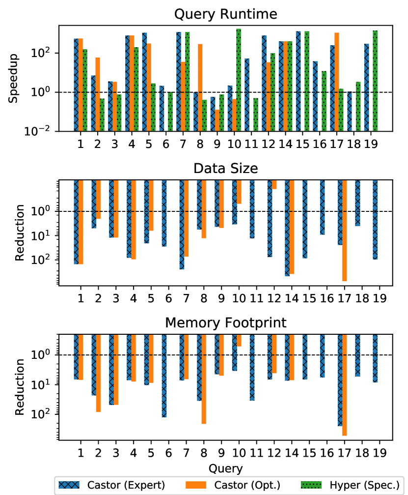
Figure 7. Performance on TPC-H queries.

When evaluating the TPC-H queries, we used the 1Gb scale factor. We ran our benchmarks on an Intel® Xeon® E5–2470 with 100Gb of memory.

Runtime. Figure 7 shows the speedup over baseline Hyper. The query runtime numbers in Table 1 show that the layouts and query code generated by Castor from expert queries are faster or significantly faster than Hyper for 15 out of 18 queries. In the cases where Castor is slower than Hyper, no query is more than 2x slower.

If Hyper is given specialized views and indexes, then its performance is on par with Castor. However, constructing and maintaining these views takes effort, and Hyper cannot assist the user in creating a collection of views which maintains the semantics of the original query.

Layout Size. We recorded the size of the layouts that Castor produced and compared them to the size of Hyper’s specialized views and indexes. Figure 7 shows that Castor’s specialized layouts are much smaller than Hyper’s, even if Hyper uses the same kind of data removal and indexing optimizations.

The layouts were generally small—less than 10Mb for 10 out of 18 queries and less than 100Mb for all but one query. The original data set, the output of the TPC-H data generator, is 1.1Gb. The size difference between Castor’s layouts and the original data supports the hypothesis that queries, even parameterized queries, rely on fairly small subsets of the whole database, making layout specialization a profitable optimization.

Memory Use. We also measured the peak memory use of the query process for Hyper and for Castor. Hyper consistently uses approximately the same amount of memory as the layout size. In some cases it uses more, presumably because it has large runtime dependencies like LLVM. In contrast, Figure 7 shows that Castor’s peak memory use is significantly lower than Hyper for all expert queries.

Cozy. We transformed our input queries into Cozy’s specification format and ran Cozy with a 6 hour timeout. In this configuration, we found that Cozy was unable to make significant improvements on all but two of the TPC-H queries. In Q4, Cozy precomputed one of the joins and a filter. In Q17, Cozy added an index. We ran both of these queries and found that despite the optimization Q4 was slower than baseline Hyper at 5.4s and Q17 was too slow to run on the entire TPC-H dataset. Although Cozy is effective at synthesizing data structures from small relational specifications, the size of the TPC-H queries causes a significant slowdown in its solver-based verification step.

Chestnut. We attempted to use Chestnut to optimize four of the TPC-H queries, but we were unable to build and run the generated code. Manually examining the selected layouts for Q1 and Q3–6, we find that Chestnut uses projection and indexes in many of the same places that Castor does, but misses some optimizations that Castor can take advantage of, such as aggregate precomputation (Sec. 4.4).

7.3. Optimizer

The performance of the automatic optimizer is mixed. In some cases, it generates queries that perform similarly or better than the expertly tuned queries. In others, it fails to find a transformation sequence that generates a serializable query, it generates a serializable query that uses a layout that is too large to compile in a reasonable amount of time, or it generates a query which performs poorly.

In most of the cases where the optimizer fails to find a solution, it fails because the cost model provided an inaccurate estimate of the performance of the candidate. In the cost model, we only consider the time required to run the query, not the size of the layout. This avoids a complex multi-variable optimization problem, but it means that the optimizer sometimes generates layouts that are too large to be compiled efficiently.

Despite the mixed performance of the optimizer, it provides a good starting point for an expert implementation, and it demonstrates that automatically optimizing programs in the layout algebra is feasible.

7.4. Summary

We showed that Castor produces artifacts that are competitive in performance and in size with a state-of-the-art in-memory database. These results show that database compilation is a compelling technique for improving query performance on static and slowly changing datasets.

8. Related Work

Deductive Synthesis. There is a long line of work that uses deductive synthesis and program transformation rules to optimize programs (Blaine et al., 1998; Puschel et al., 2005), to generate data structure implementations (Delaware et al., 2015), and to build performance DSLs (Ragan-Kelley et al., 2013; Sujeeth et al., 2014). Castor is a part of this line of work: it is a performance DSL which uses deduction rules to generate and optimize layouts. However its focus on particular data sets and on deduction rules to optimize data in addition to programs separates it from previous work.

Data Representation Synthesis. The layout optimization problem is similar to the problem of synthesizing a data structure that corresponds to a relational specification (Hawkins et al., 2010, 2011; Loncaric et al., 2016, 2018; Sujeeth et al., 2014). Castor considers a restricted version of the data structure synthesis problem where the query and the dataset are known to the compiler, which allows Castor to use optimizations which would not be safe if the data was not known. The best data structure synthesis tool—Cozy—uses an SMT solver to verify candidates, which does not scale to the TPC-H queries. Castor’s use of deduction rules avoids this costly verification step.

Database Storage. Traditional databases are mostly row-based. Column-based database systems (e.g., Hyper (Neumann, 2011), MonetDB (Boncz and Kersten, 1999) and C-Store (Stonebraker et al., 2005)) are popular for OLAP applications, outperforming row-based approaches by orders of magnitude. However, the existing work on database storage generally considers specific storage optimizations (e.g., (Ailamaki et al., 2001)), rather than languages for expressing diverse storage options. In this vein is RodentStore (Cudre-Mauroux et al., 2009), which proposed a language to express rich types of storage layouts and showed that different layouts could benefit different applications. However, a compiler was never developed to create the layouts from this language; the paper demonstrated its point by implementing each layout by hand. Also related is Chestnut: a tool for generating specialized layouts for object queries (Yan and Cheung, 2019). Chestnut has separate layout and query languages and synthesizes a query after choosing the layout. This limits its ability to use transformations that change the data, like predicate precomputation (Sec. 4.7).

There have also been studies of physical layouts for other types of data, such as for scientific data (Stonebraker, 2012), and geo-spatial data (Gutiérrez and Baumann, 2007). Although not directly comparable, we hope that Castor can be extended to support those data types.

Materialized View and Index Selection. The layouts that Castor generates are similar to materialized views, in that they store query results. Castor also generates layouts which contain indexes. Several problems related to the use of materialized views and indexes have been studied (see (Halevy, 2001) for a survey): (1) the view storage problem that decides which views need to be materialized (Chirkova and Genesereth, 2000), (2) the view selection problem that selects view(s) that can answer a given query, (3) the query rewriting problem that rewrites the given query based on the selected view(s) (Pottinger and Levy, 2000), (4) the index selection problem that selects an appropriate set of indexes for a query (Stonebraker, 1974; Gupta et al., 1997; Bruno and Chaudhuri, 2005; Talebi et al., 2008). However, materialized views are restricted to being flat relations. The layout space that Castor supports is much richer than that supported by materialized views and indexes. In addition, the view selection literature has not previously considered the problem of generating execution plans for chosen views and indexes.

Query Compilation. Castor uses techniques from the query compilation literature (Tahboub et al., 2018; Shaikhha et al., 2016; Klonatos et al., 2014). It extends these techniques by using information about the layout to specialize its queries.

9. Conclusion

We have presented Castor, a domain specific language for expressing a wide variety of physical database designs, and a compiler for this language. We have evaluated it empirically and shown that it is competitive with the state-of-the-art in memory database systems.

Appendix A Layout Semantics

In this section we discuss the layout semantics, which specifies how a layout algebra program may be serialized to a binary format.

Each of the layout operators has a serialization format that is designed to be as compact as possible. These are as follows:

• Integers are stored using the minimum number of bytes, from 1 to 8 bytes.

• Booleans are stored as single bytes.

• Fixed point numbers are normalized to a fixed scale, and stored as integers.

• Tuples are stored as the concatenation of the layouts they contain, prefixed by a length.

• Lists are stored as a length followed by the concatenation of their elements. They can be efficiently scanned through, but not accessed randomly by index.

• Hash indexes are implemented using minimal perfect hashes (Botelho et al., 2007; Davi de Castro Reis et al., 2011). The hash values are stored as in a list, but during serialization a lookup table is generated using the CMPH library and stored before the values. Using perfect hashing allows the hash indexes to have load factors up to 99%.

• Ordered indexes are similar to hash indexes in that they store a lookup table in addition to storing the values. In the case of the ordered index keys are stored sorted and the correct range is found by binary search.

Serialization proceeds in two passes. First, we compute a layout type according to the rules in Figure 8. This type is an abstraction of the layout; we use it to specialize the layout to the data that it stores. For example, we use an interval abstraction to represent integer scalars as well as lengths of collections like lists. We use these intervals to choose the number of bytes to use for these integers when serializing the layout. In some cases we are able to use this abstraction to avoid storing anything at all. For example, if we know that the length field of a tuple is always the same, we can avoid storing that field and instead bake it into the layout reading code. This is a surprisingly important optimization; for a tuple containing two integers, a naive implementation would spend a third of the tuple’s bytes just to store the length field.

After computing the layout type, we serialize the layout according to the rules in Appendix A.

$$n ::= \ \mathbb{Z}\quad r::=\ [n,n]$$

$$t ::= \ \textsf{intT}(r)~{}|~{}\textsf{boolT}~{}|~{}\textsf{fixedT}(r,n_{scale})~{}|~{}\textsf{stringT}(r_{chars})$$

— $$\ \textsf{tupleT}([t_{1},\dots,t_{k}])~{}|~{}\textsf{listT}(t,n_{elems})~{}|~{}\textsf{hash-idxT}(t_{k},t_{v})$$

— $$\ \textsf{ordered-idxT}(t_{k},t_{v})~{}|~{}\textsf{emptyT}$$

Figure 8. Syntax of the layout types.

$$\begin{aligned} \inference{\sigma|-\textsf{{scalar}}(e\mapsto n)\Downarrow x\\ x\ \text{is an integer}}{\sigma|-\textsf{{scalar}}(e\mapsto n):\textsf{intT}([x,x])}&\inference{\sigma|-q_{1}:t_{1},\dots,\sigma|-q_{k}:t_{k}\\ t=\textsf{tupleT}([t_{1},\dots,t_{k}],\tau)}{\sigma|-\textsf{{tuple}}_{\tau}([q_{1},\dots,q_{k}]):t}\end{aligned}$$

$$\begin{aligned} \inference{\sigma|-q_{k}\Downarrow r\\ t_{k}=\bigsqcup_{\sigma^{\prime}\in r,\sigma^{\prime}|-q_{v}:t^{\prime}}t^{\prime}\\ t=\textsf{listT}(t,[|r|,|r|])}{\textsf{{list}}{}(q_{k}\ \textsf{as}\ n,q_{v}):t}&\inference{t_{1}=\textsf{intT}([q_{1},h_{1}])&t_{2}=\textsf{intT}([q_{2},h_{2}])}{t_{1}\sqcup t_{2}=\textsf{intT}([\min(q_{1},q_{2}),\max(h_{1},h_{2})])}\end{aligned}$$

Figure 9. Selected semantics of the type inference pass.

Figure 10. Selected semantics of the layout serialization pass.

Appendix B Runtime Semantics

In this section we describe how layout algebra programs are compiled to executable code and how that compilation process uses the layout type.

As mentioned in Sec. 5, query code is generated as in (Tahboub et al., 2018). This method is referred to as push-based, or data-centric query evaluation. For each query operator, the code generator contains a function that emits the code that implements the operator. Rather than emitting an iterator which can be stepped forward at runtime, these functions take a callback which generates the code that consumes the output of the operator. This compilation strategy has the effect of inlining the operator implementations into a single loop nest. We found that using this strategy instead of a traditional iterator model approach is critical for getting good performance from the generated code.

The drawback of push-based query evaluation is that certain operators, such as deduplication and ordering, must buffer their inputs before processing them. Rather than implement buffering, we restrict the use of these operators and replace them with layout-based implementations wherever possible.

For each of the layout operators, we generate code that reads the layout generated by the serialization pass. This process uses the layout type to determine where to specialize the layout reading code. Essentially, for each layout specialization in Appendix A, there is a corresponding specialization of the generated code.

Appendix C Correctness of Filter Elimination

In this section we discuss the correctness of the filter elimination rule (Sec. 4.5) in detail. We show that the relational semantics is sufficiently detailed to prove the correctness of the transformation rules.

We say that two programs $q_{1}$ and $q_{2}$ are equivalent if they produce the same value in every context and we denote equivalence as $q_{1}\equiv q_{2}$ according to the following rule:

$$\inference[Equiv]{\forall\sigma,\delta,s.~{}\sigma,\delta|-q\Downarrow s\iff\sigma,\delta|-q^{\prime}\Downarrow s}{q\equiv q^{\prime}}$$

Now we prove that the filter elimination rule is semantics-preserving:

$$\inference$$

&

part(q,e,x)=(qk,qv)filter(e=e′,q)->hash-idx(qkasx,qv,e′).

Theorem C.1.

If $\textsc{part}(q,e,x)=(q_{k},q_{v})$ and $x$ is a fresh scope, then

$$\textsf{filter}(e=e^{\prime},q)\equiv\textsf{{hash-idx}}{}(q_{k}\ \textsf{as}\ x,q_{v},e^{\prime}).$$

Proof.

By Equiv, the right-hand-side of this implication is equivalent to:

$$\forall\sigma,\delta,s.~{}\sigma,\delta|-\textsf{filter}(e=e^{\prime},q)\Downarrow s\iff$$

$$\quad\sigma,\delta|-\textsf{{hash-idx}}{}(q_{k}\ \textsf{as}\ x,q_{v},e^{\prime})\Downarrow s.$$

By R-HI,

$$\sigma,\delta|-\textsf{filter}(e=e^{\prime},q)\Downarrow s\iff$$

$$\quad\sigma,\delta|-\textsf{depjoin}{}(q_{k}\ \textsf{as}\ x,\textsf{filter}{}(x.e=e^{\prime},q_{v}))\Downarrow s.$$

By the definition of partition, $q_{k}=\textsf{dedup}{}(\textsf{select}{}(\{e\},q))$ and $q_{v}=\textsf{filter}{}(x.e=e,q)$, so

$$\sigma,\delta|-\textsf{filter}(e=e^{\prime},q)\Downarrow s\iff$$

$$\quad\sigma,\delta|-\textsf{depjoin}{}(\textsf{dedup}{}(\textsf{select}{}(\{e\},q))\ \textsf{as}\ x,$$

$$\quad\quad\textsf{filter}{}(x.e=e^{\prime},\textsf{filter}{}(x.e=e,q)))\Downarrow s.$$

We can simplify the filter operators to get:

$$\sigma,\delta|-\textsf{filter}(e=e^{\prime},q)\Downarrow s\iff$$

$$\quad\sigma,\delta|-\textsf{depjoin}{}(\textsf{dedup}{}(\textsf{select}{}(\{e\},q))\ \textsf{as}\ x,$$

$$\quad\quad\textsf{filter}{}(x.e=e^{\prime}\land x.e=e,q))\Downarrow s.$$

Proving the correctness of this simplification is straightforward and does not rely on the correctness of the hash-index introduction rule.

By R-Filter and R-Depjoin (and some abuse of notation), this is equivalent to:

$$[t~{}|~{}t<-\textsf{filter}(e=e^{\prime},q)]=\left[t^{\prime}~{}\Bigg{|}~{}{\begin{array}[]{c}t<-\textsf{dedup}{}(\textsf{select}{}(\{e\},q))\\ t^{\prime}<-\textsf{filter}{}(t=e^{\prime}\land t=e,q)\end{array}}\right].$$

At this point there are two cases of interest. In the first case, assume that $e^{\prime}\in\textsf{dedup}{}(\textsf{select}{}(\{e\},q))$. By the semantics of dedup, $e^{\prime}$ will appear exactly once in this query result if it appears at all. We can conclude that

$$\left[t^{\prime}~{}\Bigg{|}~{}{\begin{array}[]{c}t<-\textsf{dedup}{}(\textsf{select}{}(\{e\},q))\\ t^{\prime}<-\textsf{filter}{}(t=e^{\prime}\land t=e,q)\end{array}}\right]$$

$$\quad=\begin{array}[]{c}[t^{\prime}~{}|~{}t^{\prime}<-\textsf{filter}(e^{\prime}=e^{\prime}\land e^{\prime}=e,q)]\mathbin{+\!\!+}{}\\ \quad[t^{\prime}~{}|~{}t\neq e^{\prime},t^{\prime}<-\textsf{filter}(e^{\prime}=t\land t=e,q)]\end{array}$$

$$\quad=[t^{\prime}~{}|~{}t^{\prime}<-\textsf{filter}(e^{\prime}=e^{\prime}\land e^{\prime}=e,q)]\mathbin{+\!\!+}{}[~{}]$$

$$\quad=[t^{\prime}~{}|~{}t^{\prime}<-\textsf{filter}(e^{\prime}=e,q)]$$

In the second case, assume that $e^{\prime}\not\in\textsf{dedup}{}(\textsf{select}{}(\{e\},q))$. In this case, there is no $e$ such that $e=e^{\prime}$, so $\textsf{filter}(e=e^{\prime},q)=[~{}]$. Similarly, there is no $t$ such that $t=e^{\prime}$, so

$$\left[t^{\prime}~{}\Bigg{|}~{}{\begin{array}[]{c}t<-\textsf{dedup}{}(\textsf{select}{}(\{e\},q))\\ t^{\prime}<-\textsf{filter}{}(t=e^{\prime}\land t=e,q)\end{array}}\right]=[~{}].$$

In both cases, the two programs are equivalent, so we can conclude that the rule is semantics-preserving. ∎

We can conclude from this proof that showing correctness for the transformation rules is feasible.

$$S ::= \ \{x_{1}\mapsto e_{1},\dots,x_{m}\mapsto e_{m}\}\quad T::=[C,\ \dots,\ q_{n}]~{}|~{}\dots~{}|~{}[q_{1},\ \dots,\ C]$$

$$C ::= \ [\cdot]~{}|~{}\textsf{select}(S,C)~{}|~{}\textsf{filter}(e,C)~{}|~{}\textsf{join}(e,q,C)~{}|~{}\textsf{group-by}(S,E,C)$$

— $$\ \textsf{dedup}(C)~{}|~{}\textsf{{list}}{}(q\ \textsf{as}\ x,C)~{}|~{}\textsf{{list}}{}(C\ \textsf{as}\ x,q)~{}|~{}\textsf{{tuple}}_{\tau}(T)$$

— $$\ \textsf{{hash-idx}}{}(C\ \textsf{as}\ x,q_{v},t_{k})~{}|~{}\textsf{{hash-idx}}{}(q_{k}\ \textsf{as}\ x,C,t_{k})$$

— $$\ \textsf{{order\-ed-idx}}{}(C\ \textsf{as}\ x,q_{v},t_{lo},t_{hi})~{}|~{}\textsf{{order\-ed-idx}}{}(q_{k}\ \textsf{as}\ x,C,t_{lo},t_{hi})$$

Figure 11. The grammar of contexts.

Figure 12. Execution semantics of the layout algebra.

$$\textsf{{hash-idx}}{}(\textsf{select}{}(\{id_{p},id_{c}\},$$

$$\quad\textsf{join}{}(enter_{p}<enter_{c}\land enter_{c}<exit_{p},$$

$$\quad\quad\textsf{select}{}(\{id\mapsto id_{p},enter\mapsto enter_{p},exit\mapsto exit_{p}\},log),$$

$$\quad\quad\textsf{select}{}(\{id\mapsto id_{c},enter\mapsto enter_{c}\},log)))\ \textsf{as}\ h,$$

$$\quad\textsf{{list}}{}(\textsf{select}{}(\{enter_{p},enter_{c}\},$$

$$\quad\quad\textsf{join}{}(enter_{p}<enter_{c}\land enter_{c}<exit_{p}\land id_{c}=h.id_{c}\land id_{p}=h.id_{p},$$

$$\quad\quad\quad\textsf{select}{}(\{id\mapsto id_{p},enter\mapsto enter_{p},exit\mapsto exit_{p}\},log),$$

$$\quad\quad\quad\textsf{select}{}(\{id\mapsto id_{c},enter\mapsto enter_{c}\},log)))\ \textsf{as}\ l,$$

$$\quad\quad\textsf{{tuple}}_{\textsf{cross}}([\textsf{{scalar}}(l.enter_{p}),\textsf{{scalar}}(l.enter_{c})])),$$

$$\quad(\$pid,\$cid))$$

Figure 13. Hash-index layout.

	Hyper				Castor (Expert)			Castor (Optimizer)
Q#	Time3	Time2	Mem.	Size	Time2	Mem.	Size	Time2	Mem.	Size
1	19.00	0.12	15.2	17.8	0.04	2.3	0.1	0.03	2.2	0.1
2 0	5.00	10.52	238.0	206.6	0.71	10.4	41.8	0.08	2.9	102.8
3 0 1	17.00	22.30	877.1	966.8	4.73	18.3	81.0	4.98	18.4	81.0
4	8.00	0.04	17.0	17.8	¡0.01	2.4	0.2	¡0.01	2.2	0.2
5	11.00	3.87	26.0	24.1	¡0.01	2.5	1.2	0.04	3.0	3.8
6	12.00	11.75	900.5	858.8	5.69	7.2	31.0	—	—	—
7	12.00	0.01	16.3	17.8	¡0.01	2.3	¡0.1	0.34	2.5	0.2
8	7.00	17.35	529.5	375.4	7.33	15.4	67.1	0.02	2.5	29.4
9	31.00	40.60	1580.2	1550.8	54.08	358.6	365.0	241.00	317.6	323.0
10 0 1	17.00	¡0.01	116.8	112.2	7.82	34.5	33.1	38.10	227.2	230.6
11	8.00	16.07	89.5	68.2	0.15	2.6	5.3	—	—	—
12	8.00	0.08	15.4	17.8	¡0.01	2.3	0.2	0.24	3.8	148.3
14	4.00	¡0.01	16.0	17.8	¡0.01	2.2	¡0.1	¡0.01	2.3	¡0.1
15	13.00	¡0.01	14.7	17.8	¡0.01	2.2	0.2	—	—	—
16 1	38.00	3.19	32.7	35.7	1.01	5.8	3.9	—	—	—
17	11.00	7.43	1238.2	1224.7	0.04	5.0	50.8	¡0.01	2.4	1.6
18 0	42.00	12.47	388.7	295.7	39.18	73.9	73.5	—	—	—
19	28.00	0.02	19.5	17.8	0.10	2.4	0.2	—	—	—

⁰ Limit clause removed. ¹ Run time ordering removed. ² Specialized. ³ Unspecialized.

Table 1. Runtime of queries derived from TPC-H (ms). Memory use is the peak resident set size during a query (Mb). Size is the layout size (Mb).

References

- (1)
- Ailamaki et al. (2001) Anastassia Ailamaki, David J. DeWitt, Mark D. Hill, and Marios Skounakis. 2001. Weaving Relations for Cache Performance. In VLDB. 169–180.
- Blaine et al. (1998) Lee Blaine, Limei Gilham, Junbo Liu, Douglas R. Smith, and Stephen Westfold. 1998. Planware-Domain-Specific Synthesis of High-Performance Schedulers. In Automated Software Engineering, 1998. Proceedings. 13th IEEE International Conference On. IEEE, 270–279.
- Boncz and Kersten (1999) Peter A. Boncz and Martin L. Kersten. 1999. MIL Primitives for Querying a Fragmented World. The VLDB Journal 8, 2 (Oct. 1999), 101–119. https://doi.org/10.1007/s007780050076
- Botelho et al. (2007) Fabiano C. Botelho, Rasmus Pagh, and Nivio Ziviani. 2007. Simple and Space-Efficient Minimal Perfect Hash Functions. In Algorithms and Data Structures: 10th International Workshop, WADS 2007 (Theoretical Computer Science and General Issues), Vol. 4619. Springer, Halifax, Canada, 139–150.
- Bruno and Chaudhuri (2005) Nicolas Bruno and Surajit Chaudhuri. 2005. Automatic Physical Database Tuning: A Relaxation-Based Approach. In Proceedings of the 2005 ACM SIGMOD International Conference on Management of Data (SIGMOD ’05). ACM, New York, NY, USA, 227–238. https://doi.org/10.1145/1066157.1066184
- Chaudhuri (1998) Surajit Chaudhuri. 1998. An Overview of Query Optimization in Relational Systems. In Proceedings of the Seventeenth ACM SIGACT-SIGMOD-SIGART Symposium on Principles of Database Systems (PODS ’98). ACM, New York, NY, USA, 34–43. https://doi.org/10.1145/275487.275492
- Cheung et al. (2013) Alvin Cheung, Armando Solar-Lezama, and Samuel Madden. 2013. Optimizing Database-Backed Applications with Query Synthesis. ACM SIGPLAN Notices 48, 6 (2013), 3–14. http://dl.acm.org/citation.cfm?id=2462180
- Chirkova and Genesereth (2000) Rada Chirkova and Michael R. Genesereth. 2000. Linearly Bounded Reformulations of Conjunctive Databases. In Computational Logic - CL 2000, First International Conference, London, UK, 24-28 July, 2000, Proceedings. 987–1001. https://doi.org/10.1007/3-540-44957-4_66
- Codd (1970) E. F. Codd. 1970. A Relational Model of Data for Large Shared Data Banks. Commun. ACM 13, 6 (June 1970), 377–387. https://doi.org/10.1145/362384.362685
- Codd (1971) Edgar F. Codd. 1971. A Data Base Sublanguage Founded on the Relational Calculus. In Proceedings of the 1971 ACM SIGFIDET (Now SIGMOD) Workshop on Data Description, Access and Control. ACM, 35–68.
- Council (2008) Transaction Processing Performance Council. 2008. TPC-H Benchmark Specification. 21 (2008), 592–603.
- Cudre-Mauroux et al. (2009) Philippe Cudre-Mauroux, Eugene Wu, and Sam Madden. 2009. The Case for RodentStore, an Adaptive, Declarative Storage System. In CIDR. arXiv:0909.1779 http://arxiv.org/abs/0909.1779
- Davi de Castro Reis et al. (2011) Davi de Castro Reis, Djamel Belazzougui, Fabiano Cupertino Botelho, and Nivio Ziviani. 2011. CMPH: C Minimal Perfect Hashing Library. http://cmph.sourceforge.net
- Delaware et al. (2015) Benjamin Delaware, Clément Pit-Claudel, Jason Gross, and Adam Chlipala. 2015. Fiat: Deductive Synthesis of Abstract Data Types in a Proof Assistant. In ACM SIGPLAN Notices, Vol. 50. ACM, 689–700.
- Graefe (1994) Goetz Graefe. 1994. Volcano/Spl Minus/an Extensible and Parallel Query Evaluation System. IEEE Transactions on Knowledge and Data Engineering 6, 1 (1994), 120–135.
- Gupta et al. (1997) H. Gupta, V. Harinarayan, A. Rajaraman, and J. D. Ullman. 1997. Index Selection for OLAP. In Proceedings 13th International Conference on Data Engineering. IEEE Computer Society, Junglee Corp., Palo Alto, CA., 208–219. https://doi.org/10.1109/ICDE.1997.581755
- Gutiérrez and Baumann (2007) Angélica García Gutiérrez and Peter Baumann. 2007. Modeling Fundamental Geo-Raster Operations with Array Algebra. In Workshops Proceedings of the 7th IEEE International Conference on Data Mining (ICDM 2007), October 28-31, 2007, Omaha, Nebraska, USA. 607–612. https://doi.org/10.1109/ICDMW.2007.53
- Halevy (2001) Alon Y. Halevy. 2001. Answering queries using views: A survey. VLDB J. 10, 4 (2001), 270–294. https://doi.org/10.1007/s007780100054
- Hawkins et al. (2010) Peter Hawkins, Alex Aiken, Kathleen Fisher, Martin Rinard, and Mooly Sagiv. 2010. Data Structure Fusion. In Programming Languages and Systems (Lecture Notes in Computer Science). Springer, Berlin, Heidelberg, 204–221. https://doi.org/10.1007/978-3-642-17164-2_15
- Hawkins et al. (2011) Peter Hawkins, Alex Aiken, Kathleen Fisher, Martin Rinard, and Mooly Sagiv. 2011. Data Representation Synthesis. In Proceedings of the 32Nd ACM SIGPLAN Conference on Programming Language Design and Implementation (PLDI ’11). ACM, New York, NY, USA, 38–49. https://doi.org/10.1145/1993498.1993504
- Jarke and Koch (1984) Matthias Jarke and Jurgen Koch. 1984. Query Optimization in Database Systems. Comput. Surveys 16, 2 (June 1984), 111–152. https://doi.org/10.1145/356924.356928
- Klonatos et al. (2014) Yannis Klonatos, Christoph Koch, Tiark Rompf, and Hassan Chafi. 2014. Building Efficient Query Engines in a High-Level Language. Proceedings of the VLDB Endowment 7, 10 (2014), 853–864. http://dl.acm.org/citation.cfm?id=2732959
- Loncaric et al. (2018) Calvin Loncaric, Michael D. Ernst, and Emina Torlak. 2018. Generalized Data Structure Synthesis. In Proceedings of the 40th International Conference on Software Engineering. ACM, 958–968.
- Loncaric et al. (2016) Calvin Loncaric, Emina Torlak, and Michael D. Ernst. 2016. Fast Synthesis of Fast Collections. In Proceedings of the 37th ACM SIGPLAN Conference on Programming Language Design and Implementation (PLDI ’16). ACM, New York, NY, USA, 355–368. https://doi.org/10.1145/2908080.2908122
- Neumann (2011) Thomas Neumann. 2011. Efficiently Compiling Efficient Query Plans for Modern Hardware. Proc. VLDB Endow. 4, 9 (June 2011), 539–550. https://doi.org/10.14778/2002938.2002940
- Pottinger and Levy (2000) Rachel Pottinger and Alon Y. Levy. 2000. A Scalable Algorithm for Answering Queries Using Views. In VLDB 2000, Proceedings of 26th International Conference on Very Large Data Bases, September 10-14, 2000, Cairo, Egypt. 484–495. http://www.vldb.org/conf/2000/P484.pdf
- Puschel et al. (2005) M. Puschel, J. M. F. Moura, J. R. Johnson, D. Padua, M. M. Veloso, B. W. Singer, Jianxin Xiong, F. Franchetti, A. Gacic, Y. Voronenko, K. Chen, R. W. Johnson, and N. Rizzolo. 2005. SPIRAL: Code Generation for DSP Transforms. Proc. IEEE 93, 2 (Feb. 2005), 232–275. https://doi.org/10.1109/JPROC.2004.840306
- Ragan-Kelley et al. (2013) Jonathan Ragan-Kelley, Connelly Barnes, Andrew Adams, Sylvain Paris, Frédo Durand, and Saman Amarasinghe. 2013. Halide: A Language and Compiler for Optimizing Parallelism, Locality, and Recomputation in Image Processing Pipelines. ACM SIGPLAN Notices 48, 6 (2013), 519–530.
- Rompf and Amin (2015) Tiark Rompf and Nada Amin. 2015. Functional Pearl: A SQL to C Compiler in 500 Lines of Code. In Proceedings of the 20th ACM SIGPLAN International Conference on Functional Programming (ICFP 2015). ACM, New York, NY, USA, 2–9. https://doi.org/10.1145/2784731.2784760
- Shaikhha et al. (2016) Amir Shaikhha, Yannis Klonatos, Lionel Parreaux, Lewis Brown, Mohammad Dashti, and Christoph Koch. 2016. How to Architect a Query Compiler. In Proceedings of the 2016 International Conference on Management of Data (SIGMOD ’16). ACM, New York, NY, USA, 1907–1922. https://doi.org/10.1145/2882903.2915244
- Stonebraker (1974) Michael Stonebraker. 1974. The choice of partial inversions and combined indices. International Journal of Parallel Programming 3, 2 (1974), 167–188. https://doi.org/10.1007/BF00976642
- Stonebraker (2012) Michael Stonebraker. 2012. SciDB: An Open-Source DBMS for Scientific Data. ERCIM News 2012, 89 (2012). http://ercim-news.ercim.eu/en89/special/scidb-an-open-source-dbms-for-scientific-data
- Stonebraker et al. (2005) Mike Stonebraker, Daniel J. Abadi, Adam Batkin, Xuedong Chen, Mitch Cherniack, Miguel Ferreira, Edmond Lau, Amerson Lin, Sam Madden, Elizabeth O’Neil, and others. 2005. C-Store: A Column-Oriented DBMS. In Proceedings of the 31st International Conference on Very Large Data Bases. VLDB Endowment, 553–564. http://dl.acm.org/citation.cfm?id=1083658
- Sujeeth et al. (2014) Arvind K. Sujeeth, Kevin J. Brown, Hyoukjoong Lee, Tiark Rompf, Hassan Chafi, Martin Odersky, and Kunle Olukotun. 2014. Delite: A Compiler Architecture for Performance-Oriented Embedded Domain-Specific Languages. ACM Trans. Embed. Comput. Syst. 13, 4s (April 2014), 134:1–134:25. https://doi.org/10.1145/2584665
- Tahboub et al. (2018) Ruby Y. Tahboub, Grégory M. Essertel, and Tiark Rompf. 2018. How to Architect a Query Compiler, Revisited. In Proceedings of the 2018 International Conference on Management of Data. ACM, 307–322.
- Talebi et al. (2008) Zohreh Asgharzadeh Talebi, Rada Chirkova, Yahya Fathi, and Matthias Stallmann. 2008. Exact and Inexact Methods for Selecting Views and Indexes for OLAP Performance Improvement. In Proceedings of the 11th International Conference on Extending Database Technology: Advances in Database Technology. ACM, 311–322. http://dl.acm.org/citation.cfm?id=1353383
- Visser (2005) Eelco Visser. 2005. A Survey of Strategies in Rule-Based Program Transformation Systems. Journal of Symbolic Computation 40, 1 (July 2005), 831–873. https://doi.org/10.1016/j.jsc.2004.12.011
- Yan and Cheung (2019) Cong Yan and Alvin Cheung. 2019. Generating Application-Specific Data Layouts for in-Memory Databases. Proceedings of the VLDB Endowment 12, 11 (2019), 1513–1525.
- Yessenov et al. (2017) Kuat Yessenov, Ivan Kuraj, and Armando Solar-Lezama. 2017. DemoMatch: API Discovery from Demonstrations. In PLDI. ACM, Barcelona, Spain, 15. https://doi.org/10.1145/3062341.3062386