Multi-Hot Compact Network Embedding

Abstract.

Network embedding, as a promising way of the network representation learning, is capable of supporting various subsequent network mining and analysis tasks, and has attracted growing research interests recently. Traditional approaches assign each node with an independent continuous vector, which will cause memory overhead for large networks. In this paper we propose a novel multi-hot compact network embedding framework to effectively reduce memory cost by learning partially shared embeddings. The insight is that a node embedding vector is composed of several basis vectors according to a multi-hot index vector. The basis vectors are shared by different nodes, which can significantly reduce the number of continuous vectors while maintain similar data representation ability. Specifically, we propose a MCNE_p model to learn compact embeddings from pre-learned node features. A novel component named compressor is integrated into MCNE_p to tackle the challenge that popular back-propagation optimization cannot propagate loss through discrete samples. We further propose an end-to-end model MCNE_t to learn compact embeddings from the input network directly. Empirically, we evaluate the proposed models over four real network datasets, and the results demonstrate that our proposals can save about 90% of memory cost of network embeddings without significantly performance decline.

1. Introduction

Nowadays, information networks are becoming ubiquitous in the real-world life, including social networks (e.g., Twitter, LinkedIn), paper citation networks (e.g., DBLP, Arxiv) and knowledge graphs (e.g., Freebase, Wikipedia). Mining valuable knowledge from these information networks is crucial to a variety of real applications in practice. A fundamental problem in the area of graph mining is learning a desirable representation vector for each node (Cao et al., 2015), which is called network embedding. The learned high-quality node representations are critically important to perform many down-streaming data mining tasks, such as node classification (Grover and Leskovec, 2016; Cui et al., 2018), social recommendation (Hu et al., 2016; Zhang et al., 2018b) and link prediction (Perozzi et al., 2014).

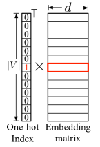
(a) One-hot index.

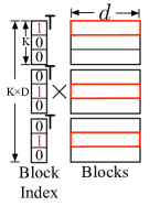
(b) KD coding.

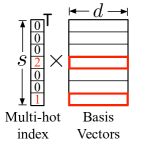
(c) Multi-hot index.

Figure 1. Comparison between three embedding strategies.

Most existing network embedding methods (Perozzi et al., 2014; Tang et al., 2015; Grover and Leskovec, 2016; Wang et al., 2016; Yang et al., 2015) encapsulate the input network into a continuous embedding matrix. Each row in the embedding matrix is the learned representation of a node. However, as each node is assigned an independent embedding vector, the size of the embedding matrix can be huge for large networks. Given a network with $|V|$ nodes and the dimension $d$ of the node embeddings, the learned embedding matrix has ($|V|\times d$) real-valued entries. When applied to downstream data mining tasks, the entire embedding matrix needs to be loaded into the memory as the lookup table, which will cause significant memory overhead. Even for a network of medium size (100,000 nodes) and $d=500$ (a popular choice), the embedding matrix has 50 million float entries , which will cost more than 1 GB memory. The high storage cost will be a key bottleneck to many memory sensitive scenarios, such as an educational application in the mobile platform may need to load the knowledge graphs to provide accurate information.

In this paper we study the novel problem of learning compact network embeddings which require much less memories while do not sacrifice the performance too much. The straightforward memory saving strategies include reducing the dimension $d$ or representing nodes with discrete vectors instead of the continuous ones such as DNE (Shen et al., 2018). However, both strategies will seriously reduce the information preserving ability of the embeddings, which leads to the significant performance sacrifice. For example, the learned embeddings from DNE are composed of binary codings instead of real-valued numbers, and thus DNE can reduce the memory cost. However, when DNE is performed in the unsupervised learning scenario, it only achieves half of the accuracy obtained by DeepWalk in node classification on Flickr and Youtube datasets (Shen et al., 2018). This is mainly because the representation ability of the binary codes is quite limited. For example in the 2-dimensional space, the binary codes can only utilize the four points ((-1,1),(1,-1),(-1,-1),(1,1)) to present the nodes, while the continuous features can exploit the whole plane to present the data.

Traditional network embedding strategies can be understood as the multiplication between the one-hot index vector and the embedding matrix as shown in Figure 1a. The major limitation of this one-hot index method is that each node needs to be represented as a unique id and an independent embedding vector, which may cause redundancy. For example if two nodes are connected and share many common neighbors, their representations tend to be similar and assigning two independent vectors for them will cause resource waste. One-hot index method needs $|V|$ continuous vectors to represent the network with $|V|$ nodes. Recently, Chen et al. (Chen et al., 2018a) proposed KD coding to reduce the memory cost of embeddings. As shown in Figure 1b, KD coding consists of D blocks and each block contains K basis vectors. For each node, KD coding firstly selects a basis vector from each block according to the block indexes, and then combines the selected D vectors as the final node representation. By sharing the basis vectors, KD coding can compose $K^{D}$ different feature vectors. A comparatively small K and D can compose into a large number of (larger than $|V|$) representation vectors. It shows that KD coding is able to significantly reduce the memory cost without much performance drop (Chen et al., 2018a). However, the introducing of blocks limits the compression capacity of KD coding because the blocks reduce the sharing ratios of the basis vectors. Each component of the final node representation can only be selected from K basis vectors in a specific block and has nothing to do with the rest K $\times$ (D-1) basis vectors in other blocks, which will cause resource waste.

To address the above issues of KD coding, in this paper we propose a multi-hot compact network embedding strategy to further improve the compression rate. Our idea is shown in Figure 1c. Each node is associated with a $s$-dimensional multi-hot index vector, where $s$ is the number of basis vectors and the sum of non-zero elements in the multi-hot index vector is $t$. The embedding vector of a node is composed by $t$ component vectors, which are selected from $s$ basis vectors according to the multi-hot index. By removing the blocks in KD coding, the proposed multi-hot index model enables each component vector of the final node representation can be selected from all the basis vectors instead of the partial ones, which improves the sharing ratios of basis vectors. Besides, each basis vector can be only selected at most once in KD coding, while our method allows duplicate selection. Given the same number of basis vectors for KD coding and the multi-hot method ($s=K\times D$ and $t=D$), the representation space of our method is $s^{t}$, while the KD coding can only achieve $(\lfloor s/t\rfloor)^{t}$.

The studied multi-hot network embedding problem is difficult to address due to the following two challenges. First, the multi-hot indexes of the nodes are trainable discrete parameters, which are difficult to be learned by existing network embedding methods. For the matrix factorization based models, it is difficult to formally define the multi-hot indexes as the discrete subjections to guide the direction of matrix factorization process (Chen et al., 2018a), while for the neural network based models, it is intractable to calculate the derivations of the discrete indexes in the back-propagation optimization process (Jang et al., 2016). Second, as a number of network embedding models have been proposed, it is time and effort efficient to directly transform the one-hot embeddings pre-learned by existing models to the multi-hot compact embeddings. A desirable multi-hot embedding framework should be able to handle both the traditional end-to-end scenario and the mentioned pre-learned feature compressing scenario.

In this paper, we propose a Multi-hot Compact Network Embedding (MCNE) framework to reduce the memory cost of the network embeddings. MCNE is a deep auto-encoder based model consisting of three components: the encoder, the compressor and the decoder. Encoder transforms the inputs to the latent vectors in the pre-defined dimension, and then feeds them into the compressor. Then the compressor generates the discrete multi-hot indexes from the latent vectors, which introduces the gumbel-softmax trick to back propagate the loss through the discrete neural nodes. Finally, decoder generates the final node representations according to the learned multi-hot indexes and the basis vectors. Specifically, we first propose the MCNE_p model to compress pre-learned one-hot index based features into the multi-hot embeddings. Considering the inputs of MCNE_p are the formatted distributed vectors, its encoder is implemented by a Multi-Layer Perceptron (MLP) to ensure the model efficiency. Then we also propose MCNE_t model for the end-to-end learning scenario. The network topology is viewed as the model input under this scenario, which is more sophisticated (e.g., sparse and high-dimensional). In order to capture the highly non-linear topology information, we introduce the graph convolutional network (GCN) as the encoder of MCNE_t. The compressor and decoder of MCNE_t are same to the ones in MCNE_p. We conduct extensive experiments over four datasets on two tasks. Experimental results demonstrate that MCNE_p can save about 90% of memory cost on average without significant performance decline, and MCNE_t outperforms the baselines with less memory cost.

We summarize our main contributions as follows.

• We propose a novel and flexible multi-hot network embedding framework MCNE, which can be applied on both scenarios of the pre-learned feature compressing and the end-to-end learning from scratch with little modifications.

• We design a novel compressor to learn discrete multi-hot indexes for the nodes, which tackles the challenge that current back-propagation optimization methods cannot propagate loss through discrete samples.

• Extensively, we evaluate the proposed models on four datasets. The results show the superior performance of our proposals by the comparison with state-of-the-art baseline methods.

The rest of this paper is organized as follows. Section 2 gives a brief review on related works. Then we formally define the studied problem in section 3. In section 4 we introduce the details of proposed MCNE_p model. The end-to-end embedding model MCNE_t is presented in section 5. Experimental results are shown and discussed in section 6. Finally, we give concluding remarks in section 7.

2. Related Work

Network embedding is closely related to the manifold learning problem (Roweis and Saul, 2000; Tenenbaum et al., 2000; Belkin and Niyogi, 2003; Li et al., 2006). Manifold learning aims to perform dimensionality reduction on the high-dimensional datasets. Traditional manifold learning methods usually convert the input dataset into a feature matrix, and then apply the matrix factorization techniques on the feature matrix to obtain the eigenvectors. Manifold learning models are usually designed for general usage, which may ignore the unique characteristics in the network topology.

Most existing network embedding models focus on encapsulating the topology information into the node representations (Zhang et al., 2018a; Pan et al., 2018; Ma et al., 2018; Kim et al., 2018; Chen et al., 2018b). The motivation is that nodes with similar topology structures (e.g., many common neighbors) should be distributed closely in the learned latent space. DeepWalk (Perozzi et al., 2014) converted the network into a set of node sequences by random walk, and then the skip-gram model was applied on the node sequences to generate node embeddings. As an improved version of DeepWalk, Node2Vec (Grover and Leskovec, 2016) proposed a more flexible loss function to capture the second-order proximity. Ribeiro et al. proposed struc2vec (Ribeiro et al., 2017) to generate the embeddings of node structural identities. SDNE (Wang et al., 2016) was a deep auto-encoder based model, which exploited the fine tuning strategy to capture the global structural information. Recently several works introduced the generative adversarial network (GAN) into network embedding learning (Dai et al., 2017; Wang et al., 2017) to stimulate the underlying true connectivity distribution over all the nodes.

Besides the network topology information, several works focused on incorporating the side information as the complementary to improve the quality of node embeddings (Tu et al., 2016; Yang et al., 2015; Li et al., 2017; Rossi et al., 2018; Liu et al., 2018; Kim et al., 2018). Tu et al. (Tu et al., 2016) extended the DeepWalk model to a max-margin extension to incorporate few available labels. Li et al. (Li et al., 2017) designed a multi-layer perceptron based model to perform semi-supervised network embedding. Yang et al. proposed TADW (Yang et al., 2015), a matrix factorization based model to fuse node attributes (text features) into the embedding process. DANE (Gao and Huang, 2018) manually calculated the correlations between structural information and the node attributes, and then integrated them into an unified objective.

Although a lot of network embedding models have been proposed, they usually suffer from high memory usage. Recently some works have focused on learning memory saving embeddings (Chen et al., 2018a; Shen et al., 2018; Zhang et al., 2018a) . DNE (Shen et al., 2018) learned binary codings as the node embeddings by adding binary subjections into the matrix factorization, which suffered from undesirable embedding quality. KD (Chen et al., 2018a) was the first work to learn compact embeddings from the pre-learned features, whose performance was limited by the block strategy. Besides, existing models are designed for a specific scenario (pre-learned feature compressing (Chen et al., 2018a) or end-to-end learning (Shen et al., 2018; Zhang et al., 2018a)), but there still lacks a more general framework that can handle both cases.

3. Problem Definition

A network is denoted as $G=\{V,T\}$, in which $V$ is the node set, and $T\in\mathbb{R}_{\{0,1\}}^{|V|\times|V|}$ is the adjacency matrix. We formally define the studied problem as follows:

Definition 3.1.

Multi-hot Compact Network Embedding. Given the input network $G$ and the representation dimension $d$, we aim to learn a multi-hot index matrix $H\in\mathbb{N}^{|V|\times s}$ and a basis matrix $B\in\mathbb{R}^{s\times d}$, where $s$ is the number of basis vectors. Each row in $B$ is a shared basis vector. Each row $H_{i}\in\mathbb{N}^{1\times s}$ in matrix $H$ represents the multi-hot index vector of the node $i$, which is under the restriction of $\sum_{j=1}^{s}H_{ij}=t$. The final embedding matrix $E\in\mathbb{R}^{|V|\times d}$ is composed by the multiplication between matrix $H$ and $B$.

The restriction of matrix $H$ ensures the embedding vector is composed by $t$ selected basis vectors (duplicate selection is allowed). The learned embedding matrix $E$ should satisfy that, in the learned latent space, the feature vectors of nodes with similar topologies would be distributed close to each other.

4. Multi-hot Network Embedding

4.1. Compact Network Embedding from Pre-learned Features

We first present the MCNE_p model which learns the multi-hot compact embeddings from the pre-learned features. We assume that the node embeddings have been learned by traditional models and applied on the industry applications. Considering that it is time and resource consuming to re-learn the embeddings of the entire network from scratch, we aim to compress the pre-learned one-hot index based embeddings with MCNE_p model. Besides, there exists various types of networks (e.g., the signed networks and attributed networks). By converting the pre-learned embeddings into the compact ones, MCNE_p can be applied on different types of networks without needing to know their unique characteristics, which proves the generality of our proposal.

Given the learned one-hot index based embedding matrix $E_{p}\in\mathbb{R}^{|V|\times d}$, we aim to learn the multi-hot index matrix $H$ and the shared basis matrix $B$ under the constraint that the multiplication of $H$ and $B$ is similar to $E$ as much as possible. This task can be viewed as the reconstruction of the original embeddings, where the auto-encoder model thrives on (Li et al., 2018). Hence we propose MCNE_p, an auto-encoder based deep model, to convert the original embeddings into the compact ones. As shown in Figure 2, the proposed MCNE_p model has three major components: encoder, compressor and decoder. Given an original embedding vector $x\in\mathbb{R}^{1\times d}$, MCNE_p will proceed the following steps.

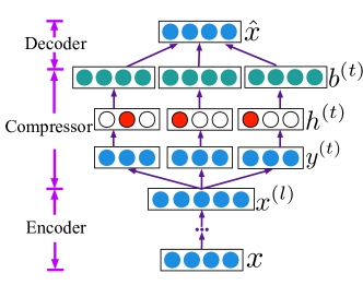
Figure 2. An illustration of the proposed MCNE_p model.

Encoder Encoder transforms the input vector $x$ to a latent vector $x^{(l)}\in\mathbb{R}^{1\times d_{l}}$, in which $l$ is the index of the top layer and $d_{l}$ is the number of neural cells in layer $l$. Formally, given the input $x$, we perform the following calculations in the encoder:

(1) $$x^{(1)} =\phi(W^{(1)}\cdot x+b^{(1)})$$

(2) $$x^{(k)} =\phi(W^{(k)}\cdot x^{(k-1)}+b^{(k)}),k=2,\cdots,l$$

where $W^{(k)}$ is the weight matrix, $b^{(k)}$ is the bias vector and $x^{(k)}$ is the learned latent vector in the $k$-th layer. $\phi$ is the activation function which introduces the nonlinearity into the feature learning process. Here we select $tanh$ as the activation function because it has stronger gradients and can avoid the bias in the gradients (LeCun et al., 2012).

Compressor Compressor learns the multi-hot index vector $h$ for the input $x$, and then selects the basis vectors according to the learned index vector. The sum of elements in the learned multi-hot index vector is $t$, which means the input $x$ can be reconstructed by $t$ basis vectors selected from all $s$ candidates according to the multi-hot indexes. Instead of directly sampling the multi-hot index vector, we sample $t$ one-hot vectors $\{h^{(1)},h^{(2)},\dots,h^{(t)}\}$ and then combine them together. The two sampling strategies are equivalent when the duplicate sampling is allowed.

As shown in the bottom of Figure 3, given the output $x^{(l)}$ from the encoder, compressor first converts it into $t$ vectors $y^{(i)}\in\mathbb{R}^{1\times s},1\leqslant i\leqslant t$. This process contains two steps: first linearly transform the $x^{(l)}$ into a $s\times t$ vector, and then reshape the learned vector to a $\mathbb{R}^{s\times t}$ matrix. The $i$-th row of the learned matrix is $y^{(i)}$:

(3) $$[y^{(1)},y^{(2)},\dots,y^{(t)}]^{\intercal}=\phi(\gamma(W^{(c)}\cdot x^{(l)}+b^{(c)}))$$

in which $\gamma$ is the reshape operation. We select $softplus$ function as the activation function $\phi$ to ensure the elements in $y^{(i)}$ are positive.

Each $y^{(i)}\in\mathbb{R}^{1\times s}$ is viewed as an independent categorical distribution, which has $s$ categories and the probability of the category $k$ is proportional to $y^{(i)}_{k}$: $\Pr(h^{(i)}_{k}=1)\propto y^{(i)}_{k}$. The sampled category $k$ represents that the $k$-th basis vector is selected. In this way, each node has its unique $t$ categorical distributions. Note that the linear transformation and the activation functions ($tanh$ and $softplus$) are all monotone functions, which ensure the vectors $y^{(i)}$ of similar nodes are also similar. Hence, similar nodes will share closer categorical distributions, leading to the similar index vectors.

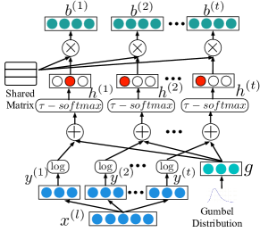
Figure 3. An illustration of the compressor.

We aim to sample a discrete parameter from each categorical distribution $y^{(i)}$ to form up the multi-hot index. For example, if the category 1 is sampled from $y^{(0)}$ and the category 4 is sampled from $y^{(1)}$, the multi-hot index will be (1, 4) and the input will be constructed by the 1-$st$ and 4-$th$ basis vectors. To tackle the challenge that back-propagation optimization cannot propagate loss through discrete samples, we introduce the gumbel-softmax trick (Maddison et al., 2016), which is a popular re-parameterization technique to generate discrete samples by adding a stochastic noise from the standard gumbel distribution.

Gumbel-softmax first samples a noise vector $g\in\mathbb{R}^{1\times s}$ from a standard gumbel distribution, and then add it with $y^{(k)}$ as $z=\log y^{(k)}+g$. We can prove the $\operatorname*{arg\,max}_{i}(z_{i})$ operation is equivalent to sampling a discrete sample from the categorical distribution $y^{(k)}$ as follows. Firstly we calculate the marginal probability when $z_{m}$ is the largest entry in $z$:

$$\Pr(\max_{i\neq m}z_{i}<z_{m})= \prod_{i\neq m}\Pr((\log y^{(k)}_{i}+g_{i})<(\log y^{(k)}_{m}+g_{m}))\noindent$$

$$= \prod_{i\neq m}\Pr(g_{i}<(\log y^{(k)}_{m}+g^{t}-\log y^{(k)}_{i}))$$

$$= \prod_{i\neq m}e^{-e^{-(z_{m}-\log y^{(k)}_{i}))}}$$

Based on the marginal distribution over $z_{m}$, we need to integrate it out to find the overall probability:

$$\Pr(m=\operatorname*{arg\,max}_{i}(z_{i}))$$

$$=\int e^{-(z_{m}-\log y^{(k)}_{m})-e^{-(z_{m}-\log y^{(k)}_{m})}}\prod_{i\neq m}e^{-e^{-(z_{m}-\log y^{(k)}_{i}))}}\mathrm{d}z_{m}$$

$$=\frac{y^{(k)}_{m}}{\sum^{s}_{i=1}y^{(k)}_{i}}$$

Hence, the distribution of the maximum element’s position in the vector $z$ is equivalent to the normalized categorical distribution $y^{(k)}$. However, $\operatorname*{arg\,max}$ operator is not differentiable, so the $\tau$-softmax function (Jang et al., 2016) is introduced as a continuous approximation of $\operatorname*{arg\,max}$ operator:

$$h^{(k)}_{i}=\frac{\text{exp}((\log(y^{(k)}_{i})+g^{i})/\tau)}{\sum_{j=1}^{s}\text{exp}((\log(y^{(k)}_{j})+g^{j})/\tau)},\quad i=1,...,s$$

where $\tau$ is the temperature parameter to control how closely the $\tau$-softmax function approximates the $\operatorname*{arg\,max}$ operation. As $\tau\to 0$, the softmax becomes an $\operatorname*{arg\,max}$ and $h^{(k)}$ is sampled from the categorical distribution $y^{(k)}$. During training, we first let $\tau>0$ to allow gradients past the neural cells, and then gradually reduce the temperature $\tau$.

As shown in the bottom right corner of Figure 3, a noise vector $g$ is sampled from a standard gumbel distribution. The gumbel distribution can be achieved from a uniform distribution by inverse transform sampling (Vogel, 2002):

(4) $$g\sim-log(-log(\text{Uniform}(0,1))).$$

Then $t$ approximate one-hot vectors $h^{(i)}\in\mathbb{R}^{1\times s}$ can be achieved by the following calculation process:

(5) $$h^{(i)}=\tau-softmax(\log(y^{(i)})+g),\quad i=1,...,t.$$

The positions of maximum entries in $h^{(i)}$ can be combined as the final multi-hot indexes. After that, $t$ basis vectors will be selected from $s$ candidates according to the sampled one-hot indexes:

(6) $$b^{(i)}=h^{(i)}\times B$$

The shared matrix $B$ contains $s$ basis vectors with the dimension of $d$. The entries of shared matrix $B$ are trainable parameters which are randomly initialized. The basis vectors will be updated in the model training step.

Decoder Given the the selected basis vectors $b^{(i)}$ from compressor, decoder composes them into the reconstructed vector $\hat{x}$. We choose the plus operation to combine the selected basis vectors:

(7) $$\hat{x}=\sum_{i=1}^{t}b^{(i)}.$$

When the learned compacting embeddings are utilized in downstream applications such as node classification, the selected basis vectors are also need to be combined as the final node representation in the same way. Hence we select the simple but fast plus operator to ensure the efficiency.

Objective Function The objective of the MCNE_p is to make the composed vector $\hat{x}$ similar to the original embedding $x$ as much as possible. We choose to use the following reconstruction loss as the objective function:

(8) $$\mathcal{L}=\frac{1}{|V|}\sum_{i=1}^{|V|}\lVert x_{i}-\hat{x}_{i}\rVert^{2}$$

Model Export After the model training finished, we need to export the basis matrix and the multi-hot index vector of each node. The matrix $B$ in the compressor is saved as the basis matrix. For each node, we can get its corresponding one-hot vectors $h^{(1)},h^{(2)},\dots,h^{(t)}$ from the compressor. For each vector $h^{(i)}$, we get the position of its maximum element as a single number: $\operatorname*{arg\,max}_{k}h^{(i)}_{k}$. After processing all the one-hot vectors, we can get $t$ integers in the range of $[1,s]$ as the multi-hot indexes of the input node. With the learned multi-hot indexes and shared basis vectors, the compact node embeddings can be easily generated following the Formula 7.

4.2. End-to-end Compact Network Embedding

In this subsection we introduce the MCNE_t model to learn the multi-hot compact network embeddings from the scratch. Given a network G with its adjacency matrix $T\in\mathbb{R}^{|V|\times|V|}$, MCNE_t aims to learn the multi-hot embeddings from the network topology directly. The input topology is more sophisticated than the pre-learned features exploited in the MCNE_p model, and thus MCNE_t should own stronger feature learning ability. Recently graph convolutional network (GCN) is popular as it nicely integrates local node features and graph topology in the convolutional layers (Kipf and Welling, 2016). GCN follows a neighborhood aggregation scheme, where the representation vector of a node is computed by recursively aggregating and transforming representation vectors of its neighboring nodes (Kipf and Welling, 2016). The original GCN is designed for the semi-supervised node classification task, while we further extend it to perform the unsupervised network embedding task. MCNE_t learns the multi-hot indexes based on the convoluted features from GCN, and utilizes the connectivity information as the indicator to guide the learning of final compact embeddings. Similar to MCNE_p, From bottom to top MCNE_t includes three major components: GCN, compressor and decoder.

GCN GCN performs convolution operation on the topology structure, which is essentially a first-order approximation of localized spectral filters on the networks (Wu et al., 2019). Given the adjacency matrix $T$, GCN performs the following operation in the $k$-th layer:

(9) $$G^{(k+1)} =\phi(\tilde{D}^{-\frac{1}{2}}\tilde{T}\tilde{D}^{-\frac{1}{2}}G^{(k)}W^{(k)}).$$

$\tilde{T}=T+I_{|V|}$ is the adjacency matrix with added self-connections, in which $I_{|V|}$ is the identity matrix. $\tilde{D}_{ii}=\sum_{j}\tilde{T}_{ij}$ and other elements in $\tilde{D}$ are zeros. $W^{(k)}$ is a layer-specific trainable weight matrix. $G^{(k)}\in\mathbb{R}^{|V|\times d_{k}}$ is the input feature matrix of $k$-th layer and $d_{k}$ is the pre-defined dimension. Usually the node attributes are viewed as the initial input matrix $G^{(0)}$. As we focus on the topology-based network embedding task, the input matrix $G^{(0)}$ is randomly initialized and its entries are viewed as the trainable parameters which can be updated in the model learning process. The proposed MCNE_t can be easily applied on the attributed networks by setting matrix $G^{(0)}$ as the node attributes. $tanh$ is selected as the activation function $\phi$. The output vector $g_{i}$ from the top layer of GCN is viewed as the latent vector of node $n_{i}$.

Compressor From the top layer $l$ of GCN we can obtain a latent feature matrix $G=G^{(l)}\in\mathbb{R}^{|V|\times d_{l}}$. Each row $g_{i}$ in $G$ is the latent vector of the corresponding node $n_{i}$. The compressor is similar to the one in MCNE_p model but only differs in the inputs. The compressor in MCNE_p considers the outputs from the encoder as the inputs, while the one in MCNE_t views the learned latent features $G$ from GCN as the inputs. From the compressor, we can obtain the multi-hot indexes of the input nodes.

Decoder Same to the one of MCNE_p, decoder selects the basis vectors according to the multi-hot indexes and adds them as the reconstructed vector. Given the input node $n_{i}$, decoder generates the reconstructed version $\hat{g}_{i}$ of the latent vector $g_{i}$. The outputs from decoder are viewed as the final compact embeddings.

Objective function The loss of MCNE_t includes two parts: a reconstruction loss $\mathcal{L}_{r}$ to ensure the reconstructed vector $\hat{g}_{i}$ should be similar to its original version $g_{i}$, and a topology-guided loss $\mathcal{L}_{t}$ to ensure the learned compact embeddings can capture the structural connectivity information.

The reconstruction loss is similar to the Formula 8. The learned compact embedding $\hat{g}_{i}$ is expected to be similar to the latent feature $g_{i}$ learned from GCN, and thus the final compact embeddings can better capture the localized topology information. This loss is formally defined as:

(10) $$\mathcal{L}_{r}=\frac{1}{|V|}\sum_{i=1}^{|V|}\lVert g_{i}-\hat{g}_{i}\rVert^{2}$$

In addition, the learned compact embeddings are also expected to preserve the connectivity structural information. Hence we design another loss function $\mathcal{L}_{t}$ to capture the connectivity information, which also contributes to learning the trainable parameters in the GCN part. Given an input node $n_{i}$, we randomly select a neighbor node of $n_{i}$ as the positive sample $pos_{i}$, and an unconnected node as the negative sample $neg_{i}$. We further propose a pairwise negative sampling based objective function $\mathcal{L}_{t}$ to maximize the difference between the two node pairs: $<n_{i},pos_{i}>$ and $<n_{i},neg_{i}>$. The similarity between the connected nodes should be larger than the similarity between unconnected nodes as much as possible. $\mathcal{L}_{t}$ is formally defined as:

(11) $$\mathcal{L}_{t}=\frac{1}{|V|}\sum_{i=1}^{|V|}-\ln(\hat{g_{i}}^{\intercal}\hat{g}_{pos_{i}}-\hat{g_{i}}^{\intercal}\hat{g}_{neg_{i}})$$

By minimizing the loss $\mathcal{L}_{t}$, we can maximize the difference between the connected nodes and unconnected ones, which captures the connectivity structural information. The final objective function of MCNE_t is the weighted combination of these two losses:

(12) $$\mathcal{L}=\mathcal{L}_{t}+\beta\cdot\mathcal{L}_{r}$$

in which $\beta$ is the hyper-parameter to control the weight of reconstruction loss. After training the model, we can obtain the multi-hot indexes of nodes and the shared basis vectors from the compressor, which can be utilized to construct the final compact embeddings.

5. Experiments

In this section, we will evaluate the performance of the proposed models on four real network datasets through two tasks.

Table 1. Statistics of the three datasets (Avg_t denotes the average number of links per node).

Dataset	Nodes	Edges	Avgt	Categories
BlogCatalog	10,312	333,983	32.39	39
DBLP	16,753	10,4371	6.23	8
Flickr	23,664	1,734,334	73.29	10
Youtube	1,138,499	2,990,443	2.63	47

Datasets We utilize four datasets to evaluate the performance of different methods. Table 1 shows the statistics of four datasets.

• BlogCatalog  In the BlogCatalog platform, users can post blogs and follow other users with similar interests. Nodes in this network are the users, and the edges are the following relationships between users. Users can join different interest groups, which are viewed as their categories.

• DBLP DBLP is an academic citation network. The nodes in the DBLP network are the manuscripts, and the edges are the citation relationships between papers. This dataset contains 16,753 papers from 8 research areas, which are viewed as the labels of the nodes.

• Flickr Flickr is an image sharing platform, in which users can post images and share them with friends. The following relationships between users form the network structure. Users also can join different interest groups, which are considered as the node categories.

• Youtube YouTube is a popular video sharing website. Users can upload videos and follow other users with similar interests, which forms a social network. In this dataset, nodes are users and labels represent the interest groups

Table 2. Parameter settings of KD ($K$ and $D$) and MCNE ($s$ and $t$).

Dataset	$K$	$D$	$s$	$t$
BlogCatalog	16	8	128	8
DBLP	16	8	128	8
Flickr	16	16	256	16
Youtube	256	32	8192	32

Baseline Methods To thoroughly evaluate the performance of our proposals, we select the following two types of baselines. We compare the proposed models with the first type of baselines as follows to evaluate the compression ability:

• DNE (Shen et al., 2018) is an end-to-end model which learns binary coding based embeddings by adding binary subjections into the matrix factorization process.

• KD (Chen et al., 2018a) is the first work to learn compact embeddings from the pre-learned features, which is the strongest baseline for compressing the embeddings.

We also adopt the second type of baselines as follows to evaluate the quality of embeddings learned by the end-to-end MCNE_t model:

• DeepWalk (Perozzi et al., 2014) first converts the network topology into a set of node sequences by random walk, and then the skip-gram model is applied on the generated node sequences to learn the node embeddings.

• LINE (Tang et al., 2015) designs two loss functions to capture the first-order and second-order proximities. We concatenate the embeddings learned by the two objectives as the node features.

• Node2Vec (Grover and Leskovec, 2016) is an extension of DeepWalk by adding the guided random walk to capture the connectivity patterns.

• SDNE (Yang et al., 2015) is a deep auto-encoder based model to capture the highly non-linear topology information. It aims to preserve both the local and global structural similarities.

Parameter Settings The dimension of the node embeddings is set to 256 (a popular choice). For DNE, the portion of the labeled nodes $\lambda$ is set to $0$ as we aim to evaluate its performance in an unsupervised manner. For DeepWalk, LINE and Node2Vec, we follow the parameter settings in the original papers. The hyper-parameter $\alpha$ in SDNE is fixed to 0.5. The number of layers and the count of neural cells in each layer of SDNE are the same as the MCNE_p model.

To conduct a fair comparison, we set the numbers of basis vectors in MCNE and KD the same, which should satisfy $s=K\times D$ and $t=D$. The settings of core parameters in MCNE ($s$ and $t$) and KD ($K$ and $D$) are shown in Table 2. For the MCNE_p model, the number of layers in the encoder and decoder is set to 2 and the node count in the hidden layer is set to $s/2$. The learning rate is set to 0.001. The parameter $\tau$ in the compressor is initialized as 1 and will decrease by 0.1 after every 100 epochs. The minimum value of $\tau$ is set to 0.5. The reconstruction weight $\beta$ in Formula 12 is set to 0.3. The batch size is set to 128 and the number of epochs is set to 500. For MCNE_p model, at the end of each epoch, we evaluate the loss on a small validation set. The parameters with the lowest validation reconstruction loss are saved. Hyper-parameters are tuned using the random search strategy on the validation dataset. For MCNE_t model, the checkpoint model with the lowest training loss will be saved as the final model. The number of GCN layers in MCNE_t is set to 2, and the number of cells in the hidden layer is set to 1000.

Evaluation methods To thoroughly evaluate the performance of different embedding methods, we select node classification and link prediction as the downstream tasks for testing. For node classification, the learned embeddings are viewed as the node features, and a one-$vs$-rest logistic regression classifier is trained to predict the node labels. $T_{r}$ percentages of nodes are randomly selected as the training set and the remaining nodes are the test samples. Following the previous work (Perozzi et al., 2014), we set $T_{r}=10\%$ for the BlogCatalog, DBLP and Flickr datasets, and $T_{r}=1\%$ for the Youtube dataset. The F1-scores ( Micro-F1 and Macro-F1) are selected as the metrics.

For link prediction, 30% of edges are randomly removed from the original network. Network embedding methods are applied on the remained subnetwork to learn node embeddings. Node pairs from the removed edges are viewed as the positive samples. We randomly sample the same number of node pairs which are not connected as the negative samples. The cosine similarity score between two nodes of a node pair is calculated based on the learned embeddings. The Area Under Curve (AUC) score is selected as the metric to evaluate the consistency between the annotations and the calculated similarity scores of the node pairs. We train each embedding method on each dataset five times and report the average results. The one-$vs$-rest classifier, F1-scores and AUC score are implemented by the scikit-learn tool.

5.1. Evaluation on Compact Embedding from Pre-learned Features

In this subsection we will evaluate the performance of our model in compact network embedding from pre-learned features. Here we only compare MCNE_p with the KD coding method, because other baselines focus on the end-to-end learning and thus are not comparable in this case. The pre-learned node features are generated by the state-of-the-art network embedding model Node2Vec. The learned compact embeddings should be similar to the original features as much as possible, which means a good compression model should achieve comparable performance to Node2Vec.

Quantitative Analysis Table 3 presents the quantitative performance of KD and MCNE_p methods, where the results of Node2Vec are also shown as the benchmarks. Besides, the numbers of parameters and the memory costs along with the corresponding compression ratios are also reported.

As shown in Figure 1a, node embeddings learned by Node2Vec consist of two parts. The first part is a $|V|\times d$ continuous embedding matrix, where $V$ is the count of nodes and $d$ is the dimension of embeddings. The second part is the one-hot indexes representing a node with an integer, and thus it contains $|V|$ integers. Overall, embeddings learned from Node2vec have ($|V|\times d+|V|$) parameters. In the python 2.7 of Linux system, the size of a float object is 16 bytes and an integer object costs 12 bytes. Thus Node2vec needs ($|V|\times d\times 16+|V|\times 12$) bytes to store the learned embeddings. The memory overhead increases linearly with the number of nodes, which brings severe challenges to the memory-sensitive applications. For the Youtube dataset, it has 292.59 million parameters and costs nearly 4GB memories.

Table 3. Performance comparison of KD and MCNE_p given the same memory costs.

	Dataset	Node2Vec	KD	MCNEp
Node	Blog.	0.371	0.353	0.369
Classi.	DBLP	0.302	0.273	0.309
(Micro-F1)	Flickr	0.358	0.331	0.354
	Youtube	0.385	0.352	0.382
Node	Blog.	0.224	0.192	0.219
Classi.	DBLP	0.126	0.101	0.124
(Macro-F1)	Flickr	0.162	0.144	0.161
	Youtube	0.306	0.267	0.301
Link	Blog.	0.781	0.752	0.784
Prediction	DBLP	0.591	0.562	0.587
(AUC)	Flickr	0.683	0.667	0.680
	Youtube	0.475	0.447	0.469
# of	Blog.	2.65	0.12	0.12 (22.08)
Parameters	DBLP	4.30	0.17	0.17 (25.29)
(Million)	Flickr	6.08	0.44	0.44 (13.82)
	Youtube	292.59	38.53	38.53 (7.59)
# of Memory	Blog.	40.40	1.44	1.44 (28.06)
(MB)	DBLP	65.63	2.03	2.03 (32.33)
	Flickr	92.71	5.33	5.33 (17.39)
	Youtube	4,460.29	448.93	448.93 (9.94)

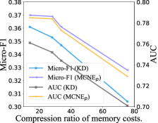
(a) Blogcatalog.

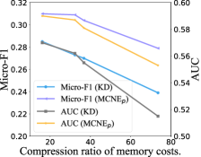
(b) DBLP.

Figure 4. Performance comparison between KD coding and MCNE_p under different compression ratios of memory cost.

As shown in the Figure 1b and Figure 1c, the numbers of parameters in the learned embeddings of MCNE_p and KD are $(s\times d+|V|\times t)$ and $(K\times D\times d+|V|\times D)$, respectively. The first part is the size of the shared basis matrix whose entries are float numbers, and the second part is the size of the learned discrete indexes which are integers. Hence the memory costs of MCNE_p and KD are $(s\times d\times 16+|V|\times t\times 12)$ bytes and $(K\times D\times d\times 16+|V|\times D\times 12)$ bytes, respectively. To ensure the fairness, the number of parameters in KD is same to MCNE_p: $s=K\times D$ and $t=D$. From the results, one can obtain the following observations:

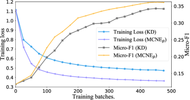
Figure 5. The training trajectories of KD and MCNE_p.

1) Compared with Node2vec, MCNE_p achieves comparable performance but the number of parameters is less than 10% of Node2vec, and also 90% memories are saved on average. By utilizing the partially shared embeddings to reduce the number of continuous basis vectors, MCNE_p consumes much less memories. In DBLP dataset, MCNE_p achieves the highest compression ratio of parameter number (25.29) and the highest memory compression ratio (32.33). MCNE_p even achieves higher Micro-F1 score than Node2vec on the DBLP dataset and higher AUC score on the BlogCatalog. This may be because the reconstruction process in the MCNE_p can work as the regularization function, which contributes to alleviating the over-fitting issue and thus improves the performance slightly.

2) Compared with the KD coding, MCNE_p achieves better performance of both tasks over all the datasets. With the same memory cost, MCNE_p outperforms KD by nearly 3% of the Micro-F1, 2.2% of the Macro-F1 and 2.5% of the AUC score. By removing the blocks, the sharing ratio of the basis vectors is increased, which contributes to improving the representation ability of MCNE_p model and leads to the better performance.

We also compare the performance of KD coding and MCNE_p under different compression ratios of memory costs. We choose different combinations of $s$ and $t$ for MCNE_p ($K$ and $D$ for KD) to obtain different compression ratios, and record the corresponding Micro-F1 and AUC scores on the Blogcatalog and DBLP datasets. Figure 4 shows the results. One can see that MCNE_p consistently outperforms KD given the same compression ratios. Besides, the compression ratio of MCNE_p is consistently larger than the ratio of KD coding when both models achieve the same Micro-F1 or AUC score, which proves MCNE_p can both reduce memory cost and learn better node embeddings. One can also see that the performance of both methods decreases with the increase of the compression ratio. A larger compression ratio means the model costs fewer memories, but leads to the lower representation capacity of the node embeddings. Thus, the tradeoff between the compression ratio and the quality of node embeddings should be carefully decided.

Learning Process Analysis Next we show the training trajectories of KD and MCNE_p by giving the loss curves of both methods on the BlogCatalog dataset as a case study. During the model training, we save the parameters after every 25 epochs and finally 20 checkpoint models can be obtained. We also record the training loss and the classification performance (Micro-F1) of each checkpoint model. The training loss represents the difference between the learned compact embeddings and the original ones. As shown in Figure 5, one can see the training loss decreases with the increase of training batches, and a smaller training loss results in a better classification performance. One can also see that compared with KD, the loss of MCNE_p is consistently smaller leading to a higher Micro-F1 score, which proves MCNE_p owns better feature learning ability.

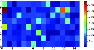
Figure 6. The utilization efficiency of the basis vectors. Numbers in the x-axis and y-axis are the indexes of basis vectors.

Utilization Efficiency Analysis on Basis Vectors Here we also analyze the utilization efficiency of basis vectors in MCNE_p on the BlogCatalog dataset. Ideally, all basis vectors should be fully utilized to convey a fraction of latent meaning. However, as the multi-hot indexes are latently defined and learned, it is possible that some basis vectors may never be used or only be used for very few times, which will cause the resource waste. We count the occurrence number of each basis vector according to the learned multi-hot indexes, and show the occurrence numbers in Figure 6. The brightness of the color in a cell is proportion to the occurrence times of the corresponding basis vector. One can see that except for several cells with very bright colors, the colors of most other cells are similar, indicating a balanced distribution of the utilization of the basis vectors. It demonstrates that the proposed MCNE_p model achieves a desirable utilization efficiency of basis vectors.

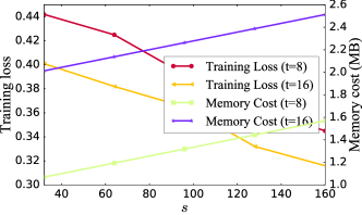
Figure 7. The parameter sensitivity study of MCNE_p.

Table 4. Performance comparison among of the end-to-end network embedding models.

	Dataset	DeepWalk	LINE	Node2Vec	SDNE	DNE	MCNEt
Node classi.	Blog.	0.351	0.347	0.371	0.387	0.207	0.397
(Micro-F1)	DBLP	0.294	0.295	0.302	0.316	0.146	0.342
	Flickr	0.324	0.335	0.358	0.369	0.161	0.381
Node classi.	Blog.	0.203	0.187	0.224	0.241	0.114	0.264
(Macro-F1)	DBLP	0.112	0.115	0.126	0.143	0.094	0.161
	Flickr	0.140	0.151	0.162	0.175	0.102	0.182
Link Pred.	Blog.	0.732	0.721	0.781	0.773	0.475	0.797
(AUC)	DBLP	0.566	0.575	0.591	0.617	0.368	0.633
	Flickr	0.628	0.645	0.683	0.692	0.385	0.706
# of para.	Blog.	2.65	2.65	2.65	2.65	2.65 (1.0)	0.12 (22.1)
(Million)	DBLP	4.30	4.30	4.30	4.30	4.30 (1.0)	0.17 (25.3)
	Flickr	6.08	6.08	6.08	6.08	6.08 (1.0)	0.44 (13.8)
# of Bytes	Blog.	40.40	40.40	40.40	40.40	0.95 (42.5)	1.44 (28.1)
(MB)	DBLP	65.63	65.63	65.63	65.63	1.54 (42.6)	2.03 (32.3)
	Flickr	92.71	92.71	92.71	92.71	4.34 (21.4)	5.33 (17.4)

Parameter Sensitivity Analysis We next perform parameter sensitivity study of MCNE_p on $s$ and $t$, where $s$ is the number of basis vectors, and $t$ represents how many basis vectors will be selected to form the final node representation. Given $t$ is set to 8 and 16, we increase $s$ from 32 to 160, and then record the training losses and the cost memories with different parameter settings. Figure 7 shows the results on the BlogCatalog dataset. One can see that the training loss decreases with the increase of $s$ or $t$, which means the learned compact embeddings becoming more and more similar to the original ones. However, a larger $s$ means more basis vectors, which will consume more memories and slow down the training speed. A larger $t$ means the final representation is composed by more basis vectors, which costs more calculation resources.

5.2. Evaluation on End-to-end Compact Network Embedding

In this subsection we evaluate the performance of the end-to-end multi-hot embedding model MCNE_t. The baselines include the traditional network embedding methods DeepWalk, LINE, Node2Vec and SDNE, and a recent memory-saving model DNE. Here we do not compare MCNE_t with KD model as KD cannot learn embeddings from the network structure directly.

Quantitative Analysis Table 4 presents the results of different embedding models along with their parameter numbers and memory costs. From the results, we can obtain the following observations:

1) Compared with the traditional embedding methods, MCNE_t achieves better performance with much fewer parameters and memory usages on all three datasets. Specifically, MCNE_t outperforms the best baseline SDNE by 2.5% on the Micro-F1 classification score with the compression ratio of nearly 20 on average. Given a center node, GCN utilizes the weighted aggregates of the features from its neighbors to generate its new representation, which can incorporate the localized topology information to improve the quality of learned embeddings. By introducing the deep GCN model with stronger feature learning ability, MCNE_t outperforms baselines on both datasets. Overall, MCNE_t can directly learn the multi-hot compact embeddings under the end-to-end scenario, which saves more than 90% memories while achieves desirable performance.

2) DNE learns the binary codings as the node embeddings. The size of the learned embedding matrix is same to the traditional methods. Hence, the count of parameters in the learned embeddings of DNE is $(|V|\times d+|V|)$. The binary entry can be represented by a bit (0 and 1), while the float number need 16 Bytes (128 bits) in Python. Thus DNE has the minimum memory cost. However, DNE performs the worst on node classification and link prediction, indicating the learned embedding quality is relatively poor. This is reasonable as the binary coding based vectors cannot preserve as much information as the continuous ones. Different from DNE reduces memory cost by learning binary codings, MCNE_t learns partially shared embeddings to reduce the number of continuous vectors, hence MCNE_t has the minimal number of parameters.

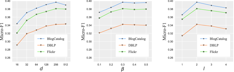
Figure 8. The parameter sensitivity of MCNE_t.

Parameter Sensitivity Analysis We next study the performance sensitivities of MCNE_t on the number of GCN layers $l$, the dimension $d$ of the learned embeddings and the reconstruction weight $\beta$. The performance of MCNE_t on different combinations of $s$ and $t$ is similar to the MCNE_p model, which has been discussed in the previous subsection. As the Micro-F1, Macro-F1 and AUC scores present similar curves with the change of core parameters, we only report the Micro-F1 score due to space limitation.

The results are shown in Figure 8. One can see that, with the increase of the dimension $d$, the Micro-F1 scores first increase and then keep stable. It demonstrates that a larger embedding dimension can provide stronger representation ability when $d$ is comparatively small. But when $d$ is too large, the model will encounter the performance bottleneck. For the parameter $\beta$, one can see that with the increase of $\beta$, the Micro-F1 scores first increase and then keep stable. It shows that incorporating appropriate reconstruction loss can better preserve the localized topology information from GCN, which contributes to improving the model performance. Finally for the number of GCN layers $l$, the performance of MCNE_t first increases then decreases. Given a center node, MCNE_t model with $l$ GCN layers can aggregate the features of its $l$-hop neighbors to learn the representation. An appropriate $l$ value contributes to learning better node representations, but a too large $l$ may introduce noises from long distance neighbors, and thus hurts the performance.

6. Conclusion

In this paper, we propose a multi-hot compact network embedding framework to learn the memory-saving node representations. We view each node representation as the combination of several basis vectors. By sharing basis vectors among different nodes, the proposed multi-hot strategy can reduce the number of continuous vectors, which further reduces the memory overhead. A deep auto-encoder based model MCNE_p integrated with a novel component named compressor is proposed to learn compact embeddings from pre-learned node features. We further propose a graph convolutional network based model MCNE_t to learn compact embeddings in the end-to-end manner. Experimental results on four real networks demonstrate the significant effectiveness of our proposals.

References

- (1)
- Belkin and Niyogi (2003) Mikhail Belkin and Partha Niyogi. 2003. Laplacian eigenmaps for dimensionality reduction and data representation. Neural computation 15, 6 (2003), 1373–1396.
- Cao et al. (2015) Shaosheng Cao, Wei Lu, and Qiongkai Xu. 2015. Grarep: Learning graph representations with global structural information. In CIKM. ACM, 891–900.
- Chen et al. (2018b) Haochen Chen, Bryan Perozzi, Yifan Hu, and Steven Skiena. 2018b. Harp: Hierarchical representation learning for networks. In AAAI.
- Chen et al. (2018a) Ting Chen, Martin Renqiang Min, and Yizhou Sun. 2018a. Learning K-way D-dimensional Discrete Codes for Compact Embedding Representations. arXiv preprint arXiv:1806.09464 (2018).
- Cui et al. (2018) Peng Cui, Xiao Wang, Jian Pei, and Wenwu Zhu. 2018. A survey on network embedding. TKDE (2018).
- Dai et al. (2017) Quanyu Dai, Qiang Li, Jian Tang, and Dan Wang. 2017. Adversarial Network Embedding. arXiv preprint arXiv:1711.07838 (2017).
- Gao and Huang (2018) Hongchang Gao and Heng Huang. 2018. Deep Attributed Network Embedding.. In IJCAI. 3364–3370.
- Grover and Leskovec (2016) Aditya Grover and Jure Leskovec. 2016. node2vec: Scalable feature learning for networks. In KDD. ACM, 855–864.
- Hu et al. (2016) Qingbo Hu, Sihong Xie, Shuyang Lin, Senzhang Wang, and S Yu Philip. 2016. Clustering Embedded Approaches for Efficient Information Network Inference. Data Science and Engineering 1, 1 (2016), 29–40.
- Jang et al. (2016) Eric Jang, Shixiang Gu, and Ben Poole. 2016. Categorical reparameterization with gumbel-softmax. arXiv preprint arXiv:1611.01144 (2016).
- Kim et al. (2018) Junghwan Kim, Haekyu Park, Ji-Eun Lee, and U Kang. 2018. Side: Representation learning in signed directed networks. In WWW. 509–518.
- Kipf and Welling (2016) Thomas N Kipf and Max Welling. 2016. Semi-supervised classification with graph convolutional networks. arXiv preprint arXiv:1609.02907 (2016).
- LeCun et al. (2012) Yann A LeCun, Léon Bottou, Genevieve B Orr, and Klaus-Robert Müller. 2012. Efficient backprop. In Neural networks: Tricks of the trade. Springer, 9–48.
- Li et al. (2018) Chaozhuo Li, Senzhang Wang, Lifang He, Philip S Yu, and Zhoujun Li. 2018. SSDMV: Semi-supervised Deep Social Spammer Detection by Multi-View Data Fusion. In ICDM.
- Li et al. (2017) Chaozhuo Li, Senzhang Wang, Dejian Yang, Zhoujun Li, Yang Yang, and Xiaoming Zhang. 2017. Semi-Supervised Network Embedding. In DASFAA. Springer, 131–147.
- Li et al. (2006) Ping Li, Trevor J Hastie, and Kenneth W Church. 2006. Very sparse random projections. In KDD. ACM, 287–296.
- Liu et al. (2018) Jie Liu, Zhicheng He, Lai Wei, and Yalou Huang. 2018. Content to node: Self-translation network embedding. In KDD. ACM, 1794–1802.
- Ma et al. (2018) Jianxin Ma, Peng Cui, Xiao Wang, and Wenwu Zhu. 2018. Hierarchical taxonomy aware network embedding. In KDD. ACM, 1920–1929.
- Maddison et al. (2016) Chris J Maddison, Andriy Mnih, and Yee Whye Teh. 2016. The concrete distribution: A continuous relaxation of discrete random variables. arXiv preprint arXiv:1611.00712 (2016).
- Pan et al. (2018) Shirui Pan, Ruiqi Hu, Guodong Long, Jing Jiang, Lina Yao, and Chengqi Zhang. 2018. Adversarially regularized graph autoencoder for graph embedding. arXiv preprint arXiv:1802.04407 (2018).
- Perozzi et al. (2014) Bryan Perozzi, Rami Al-Rfou, and Steven Skiena. 2014. Deepwalk: Online learning of social representations. In KDD. ACM, 701–710.
- Ribeiro et al. (2017) Leonardo FR Ribeiro, Pedro HP Saverese, and Daniel R Figueiredo. 2017. struc2vec: Learning node representations from structural identity. In KDD. ACM, 385–394.
- Rossi et al. (2018) Ryan A Rossi, Rong Zhou, and Nesreen K Ahmed. 2018. Deep inductive network representation learning. In WWW. 953–960.
- Roweis and Saul (2000) Sam T Roweis and Lawrence K Saul. 2000. Nonlinear dimensionality reduction by locally linear embedding. science 290, 5500 (2000), 2323–2326.
- Shen et al. (2018) Xiaobo Shen, Shirui Pan, Weiwei Liu, Yew-Soon Ong, and Quan-Sen Sun. 2018. Discrete Network Embedding.. In IJCAI. 3549–3555.
- Tang et al. (2015) Jian Tang, Meng Qu, Mingzhe Wang, Ming Zhang, Jun Yan, and Qiaozhu Mei. 2015. Line: Large-scale information network embedding. In WWW. ACM.
- Tenenbaum et al. (2000) Joshua B Tenenbaum, Vin De Silva, and John C Langford. 2000. A global geometric framework for nonlinear dimensionality reduction. science 290, 5500 (2000), 2319–2323.
- Tu et al. (2016) Cunchao Tu, Weicheng Zhang, Zhiyuan Liu, and Maosong Sun. 2016. Max-margin DeepWalk: discriminative learning of network representation. In IJCAI. 3889–3895.
- Vogel (2002) Curtis R Vogel. 2002. Computational methods for inverse problems. Vol. 23. Siam.
- Wang et al. (2016) Daixin Wang, Peng Cui, and Wenwu Zhu. 2016. Structural deep network embedding. In KDD. ACM, 1225–1234.
- Wang et al. (2017) Hongwei Wang, Jia Wang, Jialin Wang, Miao Zhao, Weinan Zhang, Fuzheng Zhang, Xing Xie, and Minyi Guo. 2017. GraphGAN: Graph Representation Learning with Generative Adversarial Nets. arXiv preprint arXiv:1711.08267 (2017).
- Wu et al. (2019) Zonghan Wu, Shirui Pan, Fengwen Chen, Guodong Long, Chengqi Zhang, and Philip S Yu. 2019. A comprehensive survey on graph neural networks. arXiv preprint arXiv:1901.00596 (2019).
- Yang et al. (2015) Cheng Yang, Zhiyuan Liu, Deli Zhao, Maosong Sun, and Edward Y Chang. 2015. Network Representation Learning with Rich Text Information.. In IJCAI. 2111–2117.
- Zhang et al. (2018b) Daokun Zhang, Jie Yin, Xingquan Zhu, and Chengqi Zhang. 2018b. Network representation learning: A survey. IEEE transactions on Big Data (2018).
- Zhang et al. (2018a) Zhengyan Zhang, Cheng Yang, Zhiyuan Liu, Maosong Sun, Zhichong Fang, Bo Zhang, and Leyu Lin. 2018a. COSINE: Compressive Network Embedding on Large-scale Information Networks. arXiv preprint arXiv:1812.08972 (2018).