Unconventional Field-Induced Spin-Density-Wave Phases in Quasi-One-Dimensional Conductors in High Magnetic Fields

Abstract

It is known that the Field-Induced Spin-Density-Wave (FISDW) phases are experimentally observed in the quasi-one-dimensional (Q1D) organic conductors with chemical formula (TMTSF)₂X (X=PF₆, ClO₄, etc.) and some others in moderate magnetic fields. From a theoretical point of view, they appear as a result of ”one-dimensionalization” of the Q1D electron spectra due to the orbital electron effect in a magnetic field. We predict that the novel FISDW phases with different physical meaning have to appear in inclined high magnetic fields in Q1D conductors as a result of combination of the spin-splitting and orbital electron effects. We suggest performing the corresponding experiments in the (TMTSF)₂X materials.

We recall that the so-called Field-Induced Spin-Density-Wave (FISDW) phases and related 3D quantum Hall effect (3D QHE) are experimentally observed in a number of Q1D organic conductors [1,2]. The most studied among them are compounds with chemical formula (TMTSF)₂X (X=PF₆, ClO₄, etc.), where the above mentioned phenomena were first discovered [3,4]. Theory of the FISDW phases was successfully developed in Refs.[5-15], whereas the 3D-QHE was considered in Refs.[13,14].

It is known [7,1,2,5,6] that electron spectrum of the Q1D organic conductors (TMTSF)₂X can be well described by the following tight-binding approximation:

$$\epsilon^{\pm}({\bf p})=\pm v_{F}(p_{x}\mp p_{F})-2t_{b}\cos(p_{y}b^{*})$$

$$-2t^{\prime}_{b}\cos(2p_{y}b^{*})-2t_{c}\cos(p_{z}c^{*}).$$ (1)

[Here, $p_{F}$ and $v_{F}$ are the electron Fermi momentum and Fermi velocity along the conducting axis ${\bf a^{*}}$, $t_{b}$ and $t_{c}$ are the electron wave functions overlapping integrals along axes ${\bf b^{*}}$ and ${\bf c^{*}}$, respectively, and the term with $t^{\prime}_{b}$ appears due to non-linearity of the real Q1D electron spectrum along ${\bf a}$ axis [7,6] ($p_{F}v_{F}\gg t_{b}\gg t^{\prime}_{b},t_{c}$)]. It is important that, for $t^{\prime}_{b}=0$, the electron spectrum (1) possesses the so-called ”nesting” property [7,1,2,5,6],

$$\epsilon_{\sigma}^{+}(\Delta p_{x},p_{y},p_{z})+\epsilon_{-\sigma}^{-}(\Delta p_{x},p_{y}+\pi/b^{*},p_{z}+\pi/c^{*})=0,$$ (2)

which allows to stabilize Spin-Density-Wave (SDW) phase due to the Peierls instability with wave vector [7,2,5,6]:

$$Q_{0}=(2p_{F},\pi/b^{*},\pi/c^{*}),$$ (3)

where $\sigma=+(-)$ for electron spin up(down), respectively.

We stress that the so-called ”anti-nesting” term, $2t^{\prime}_{b}\cos(2p_{y}b^{*})$, in Eq.(1) destroys [7,1,2,5,6] the ”nesting” condition (2) and, therefore, for high enough values of the parameter $t^{\prime}_{b}$, metallic or superconducting phases can become the ground states. In this case, as experimentally shown in Refs.[3,4], the physical situation is very interesting in a magnetic field applied along axis ${\bf c^{*}}$: a cascade of the numerous FISDW phases occurs with Hall conductivity being quantized. In theoretical works [5-15], it was shown that the ”one-dimensionalized” [5] orbital electron motion in the magnetic field restores the Peierls instability and these FISDW phases were interpreted as the SDW phases with the following quantized wave vectors:

$$Q_{n}=(2p_{F}+n\ \omega_{c}/v_{F},\pi/b^{*},\pi/c^{*}),$$ (4)

where $n$ is an integer.

Note that, using the linearized Q1D electron spectrum (1), it is possible to come to the conclusion [5,6,8-15] that the Pauli spin-splitting effect plays no role in physical properties of the FISDW phases. Very recently, we have shown [16] that, due to non-linearity of the electron spectrum along the conducting axis ${\bf a^{*}}$, the Pauli spin-splitting effect generates a new ”anti-nesting” term in the Q1D spectrum (1). In particular, in Ref.[16], we have demonstrated that this term results in a destruction of the SDW phase in a parallel magnetic field, ${\bf H}\parallel{\bf a^{*}}$ (i.e., in the absence of the orbital effect).

The goal of our Rapid Communication is to show that the above mentioned new ”anti-nesting” term [16], which is proportional to a strength of a magnetic field, is responsible for even more interesting phenomenon - a novel cascade of the FISDW phases in high magnetic fields. Unlike the known FISDW phases, the new ones have to appear due to simultaneous actions of the Pauli spin-splitting and orbital electron effects. We suggest to observe the novel FISDW phases in the organic conductors from chemical family (TMTSF)₂X in an inclined with respect to the conducting axis ${\bf a^{*}}$ magnetic field. In particular, we show that, unlike the known cascade of the FISDW phases [1-15], where the FISDW phase boundaries are roughly periodic with an inverse magnetic field, positions of the novel FISDW phases do not depend on a strength of the magnetic field. Below, they are shown to depend almost periodically on an inverse sinusoidal function of the inclination angle, $1/\sin\alpha$.

For further development, we consider the following 2D non-linearized model of Q1D spectrum in a parallel to the conducting ${\bf a^{*}}$ axis magnetic field,

$$\epsilon_{\sigma}({\bf p})=-2t_{a}\cos(p_{x}a^{*}/2)-2t_{b}\cos(p_{y}b^{*})-\mu_{B}\sigma H,$$ (5)

where $t_{a}$ is overlapping integral of electron wave functions along the conducting ${\bf a^{*}}$ axis. [Note that the first ”anti-nesting” term, $2t^{\prime}_{b}\cos(2p_{y}b^{*})$, appears later as a result of a non-linearity of the spectrum (5) with respect to variable $p_{x}$.] Contrary to the all existing theories of the FISDW phases [5,6,8-15], below we take account of both linear and quadratic terms of the variables $(p_{x}\pm p_{F})$ near two pieces of the Fermi surface in a parallel magnetic field:

$$\epsilon^{\pm}(p_{x})=\pm v_{F}(p_{x}\mp p_{F})+\gamma(p_{x}\mp p_{F})^{2},$$ (6)

where in the (TMTSF)₂X compounds [1,2,7,16]

$$v_{F}=\frac{t_{a}a^{*}}{\sqrt{2}},\ \ \ p_{F}=\frac{\pi}{2a^{*}},\ \ \ \gamma=\frac{t_{a}(a^{*})^{2}}{4\sqrt{2}}.$$ (7)

Using Eqs.(5)-(7), it is easy to demonstrate that, in a parallel magnetic field, near two sheets of the FS the electron spectrum can be written as

$$\epsilon^{\pm}_{\sigma}({\bf p})=\pm v_{F}(p_{x}\mp p_{F})+t^{\pm}_{b}(p_{y},\sigma)-\mu_{B}\sigma H+\Delta\epsilon,$$

$$t^{\pm}_{b}(p_{y},\sigma)=-2t_{b}\cos(p_{y}b^{*})+2t^{\prime}_{b}\cos(2p_{y}b^{*})$$

$$+2t_{H}\sigma\cos(p_{y}b^{*}),$$ (8)

where $t_{H}=\mu_{B}Ht_{b}/(\sqrt{2}t_{a}),\ t^{\prime}_{b}=t^{2}_{b}/(2\sqrt{2}t_{a}),\ \Delta\epsilon=\mu^{2}_{B}H^{2}/(2\sqrt{2}t_{a})$.

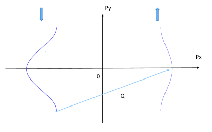
Figure 1: Left and right parts of the Q1D Fermi surface, given by Eq.(8) at $t^{\prime}_{b}=0$, are shown for different directions of electron spins (i.e., for the SDW paring). As seen, that even in this case, where the traditional ”anti-nesting” term disappears, there appears the second ”anti-nesting” term, which destroys the ”nesting” properties of the Q1D spectrum for any SDW wave-vector ${\bf Q}$.

It is important that Eq.(8) contains two kinds of ”anti-nesting” terms for the SDW instability (pay attention that the second term does not exist for a CDW case and, thus, does not destroy the CDW phase). The first of them is usual, $2t^{\prime}_{b}\cos(2p_{y}b^{*})$, which is responsible for the standard FISDW cascade of phase transitions and 3D QHE [5-15], provided the magnetic field has a finite ${\bf c^{*}}$ axis component The second ”anti-nesting” term, $2t_{H}\sigma\cos(p_{y}b^{*})$ (see Fig.1), has magnetic field dependent amplitude, $t_{H}\sim H$, which as we show generates the novel FISDW phases in high magnetic fields. In contrast, terms $-\mu_{B}H$ and $\Delta\epsilon$ in Eq.(8) do not affect seriously the FISDW phases. Indeed, term $-\mu_{B}H$ disappears for the SDW pairing, whereas term $\Delta\epsilon$ just shifts the wave vectors of the FISDW phases. Therefore, we omit the last two terms in our further calculations.

We stress that the geometry suggested by us for observations of the novel FISDW phases is different from the standard one [5,6,8-15] as well as different from that in Ref.[16]. In our case, we have strong magnetic field, which is characterized by both finite ${\bf a^{*}}$ and ${\bf c^{*}}$ axes components:

$${\bf H}=(H\cos\alpha,0,H\sin\alpha),$$ (9)

$${\bf A}=(0,Hx\sin\alpha,Hy\cos\alpha),$$ (10)

where $\alpha$ is angle between magnetic field ${\bf H}$ and ${\bf a^{*}}$ axis. Under such experimental conditions, we have both the Pauli spin-splitting effect (8) and the orbital one [5-15]. Below, we introduce the orbital effect by means of the so-called Peierls substitution method, as it is done in Ref.[5]:

$$p_{x}\mp p_{F}\rightarrow-i\frac{d}{dx},\ \ \ p_{y}b^{*}\rightarrow p_{y}b^{*}-\frac{e}{c}A_{y}b^{*}$$

$$=p_{y}b^{*}-\frac{\omega_{c}(\alpha)x}{v_{F}},\ \ \ \omega_{c}(\alpha)=\frac{ev_{F}b^{*}H\sin\alpha}{c}.$$ (11)

Let us introduce slow varying parts, $g^{\pm\pm}(i\omega_{n},p_{y};x,x_{1};\sigma)$, of the non-interacting electron Green’s functions near two open sheets of the Q1D FS, $G^{\pm\pm}(i\omega_{n},p_{y};x,x_{1};\sigma)$, by the following equations:

$$G^{++}(i\omega_{n},p_{y};x,x_{1};\sigma)=e^{ip_{F}(x-x_{1})}$$

$$\times g^{++}(i\omega_{n},p_{y};x,x_{1};\sigma),$$ (12)

$$G^{--}(i\omega_{n},p_{y};x,x_{1};\sigma)=e^{-ip_{F}(x-x_{1})}$$

$$\times g^{--}(i\omega_{n},p_{y};x,x_{1};\sigma),$$ (13)

where $\omega_{n}$ is the Matsubara’s frequency [17]. Then, using Eqs.(8) and (11), it is possible to make sure that the slow varying parts of the electron Green’s functions obey the equations:

$$\biggl{\{}i\omega_{n}+iv_{F}\frac{d}{dx}-t^{+}_{b}\biggl{[}p_{y}b^{*}-\frac{\omega(\alpha)x}{v_{F}},\sigma\biggl{]}\biggl{\}}$$

$$\times g^{++}(i\omega_{n},p_{y};x,x_{1};\sigma)=\delta(x-x_{1})\ ,$$ (14)

$$\biggl{\{}i\omega_{n}-iv_{F}\frac{d}{dx}-t^{-}_{b}\biggl{[}p_{y}b^{*}-\frac{\omega(\alpha)x}{v_{F}},\sigma\biggl{]}\biggl{\}}$$

$$\times g^{--}(i\omega_{n},p_{y};x,x_{1};\sigma)=\delta(x-x_{1})\ ,$$ (15)

where $\delta(x-x_{1})$ is the Dirac’s delta-function. It is important that the equations for slow varying parts of the Green’s functions of non-interacting electrons in a magnetic field (14) and (15) can be exactly solved:

$$g^{++}(i\omega_{n},p_{y};x,x_{1};\sigma)=\frac{sgn(\omega_{n})}{iv_{F}}\exp\biggl{\{}-\frac{\omega_{n}(x-x_{1})}{v_{F}}$$

$$-\frac{i}{v_{F}}\int^{x}_{x_{1}}t^{+}_{b}\biggl{[}p_{y}b^{*}-\frac{\omega(\alpha)u}{v_{F}},\sigma\biggl{]}du\biggl{\}},\ \omega_{n}(x-x_{1})>0,$$ (16)

$$g^{--}(i\omega_{n},p_{y};x,x_{1};\sigma)=\frac{sgn(\omega_{n})}{iv_{F}}\exp\biggl{\{}\frac{\omega_{n}(x-x_{1})}{v_{F}}$$

$$+\frac{i}{v_{F}}\int^{x}_{x_{1}}t^{-}_{b}\biggl{[}p_{y}b^{*}-\frac{\omega(\alpha)u}{v_{F}},\sigma\biggl{]}du\biggl{\}},\ \omega_{n}(x-x_{1})<0.$$ (17)

Here, we calculate a linear response of electrons to the external field, corresponding to the following SDW electron-hole pairing,

$$\hat{h}({\bf Q})=(\hat{\sigma}_{x})_{\alpha\beta}\ \exp(i{\bf Q}{\bf r})\ ,$$ (18)

in a similar way as it is done in Ref.[5] for different Q1D spectrum without the magnetic field dependent term. In random phase approximation, we obtain the so-called Stoner equation for susceptibility:

$$\chi({\bf Q})=\frac{\chi_{0}({\bf Q})}{[1-g\chi_{0}({\bf Q})]}.$$ (19)

In Eq.(19), $g$ is the effective SDW electron coupling constant, $\chi_{0}({\bf Q})$ is a susceptibility of the non-interacting electrons in a magnetic field:

$$\chi_{0}(\approx 2p_{F},Q_{y},\pi/c^{*})=T\sum_{\omega_{m}}\sum_{\sigma}\int\frac{dp_{y}}{2\pi}\int dx_{1}$$

$$\times g^{++}(i\omega_{n},p_{y};x,x_{1};\sigma)\ g^{--}(i\omega_{n},p_{y}-Q_{y};x_{1},x;-\sigma).$$ (20)

Let us substitute the known slow varying parts of the electron Green’s functions in a magnetic field (16) and (17) in Eqs.(20) and (19). As a result of straightforward but lengthy calculations, we obtain the following equation of a stability for the FISDW phases in the presence of the orbital and Pauli spin-splitting effects:

$$\frac{1}{g}=\max_{(k,\Delta t)}\int^{\infty}_{\frac{v_{F}}{\Omega}}\frac{2\pi T_{c}dz}{v_{F}\sinh\biggl{(}\frac{2\pi T_{c}z}{v_{F}}\biggl{)}}\biggl{<}\cos\biggl{\{}\biggl{[}\frac{8\Delta t}{\omega_{c}(\alpha)}\biggl{]}\sin\biggl{[}\frac{\omega_{c}(\alpha)z}{2v_{F}}\biggl{]}$$

$$\times\sin(p_{y}b^{*})-\biggl{[}\frac{4t^{\prime}_{b}}{\omega_{c}(\alpha)}\biggl{]}\sin\biggl{[}\frac{\omega_{c}(\alpha)z}{v_{F}}\biggl{]}\cos(2p_{y}b^{*})-kz\biggl{\}}$$

$$\times\cos\biggl{\{}\biggl{[}\frac{8t_{H}}{\omega_{c}(\alpha)}\biggl{]}\sin\biggl{[}\frac{\omega_{c}(\alpha)z}{2v_{F}}\bigg{]}\cos(p_{y}b^{*})\biggl{\}}\biggl{>}_{p_{y}}.$$ (21)

[Here, $Q_{x}=2p_{F}+k$, $Q_{y}=\pi/b^{*}+q\ (qb^{*}\ll 1)$, $\Delta t=t_{b}qb^{*}/2$, and $\Omega$ is a cutoff energy; $<...>_{p_{y}}$ stands for averaging procedure over variable $p_{y}$]. We stress that, in Eq.(21), we maximize SDW transition temperature, $T_{c}$, with respect to longitudinal, $k$, and transverse, $q$, wave vectors under the condition that $t_{b}\gg t^{\prime}_{b}$.

It is important that Eq.(21), derived in our Rapid Communication, is the most general equation to determine the appearance of the FISDW phases in a Q1D conductor in a magnetic field. In particular, at low enough magnetic fields, we can disregard the Pauli spin-splitting effect and, therefore, at $t_{H}=0$ and $\alpha=\pi/2$, Eq.(21) coincides with the main equation of Ref.[10]. Our current goal is not a full analysis of Eq.(21), which is difficult numerical problem and hopefully will be solved in the future. In the Rapid Communication, we consider high magnetic field limit of Eq.(21) to demonstrate novel phenomenon - the appearance of high magnetic field FISDW phases due to the the combination of the orbital electron motion and Pauli spin-splitting effects. To this end, let us consider high magnetic fields, where

$$\omega_{c}(\alpha)\geq 4t^{\prime}_{b}.$$ (22)

It is easy to see that, in this limit, the master Eq.(21) can be rewritten as

$$\frac{1}{g}=\max_{(k,\Delta t)}\int^{\infty}_{\frac{v_{F}}{\Omega}}\frac{2\pi T_{c}dz}{v_{F}\sinh\biggl{(}\frac{2\pi T_{c}z}{v_{F}}\biggl{)}}\biggl{<}\cos\biggl{\{}\biggl{[}\frac{8\Delta t}{\omega_{c}(\alpha)}\biggl{]}$$

$$\times\sin\biggl{[}\frac{\omega_{c}(\alpha)z}{2v_{F}}\biggl{]}\sin(p_{y}b^{*})-kz\biggl{\}}$$

$$\times\cos\biggl{\{}\biggl{[}\frac{8t_{H}}{\omega_{c}(\alpha)}\biggl{]}\sin\biggl{[}\frac{\omega_{c}(\alpha)z}{2v_{F}}\bigg{]}\cos(p_{y}b^{*})\biggl{\}}\biggl{>}_{p_{y}}.$$ (23)

Let us simplify the integral (23), using some well known trigonometric equations. As a result of rather simple calculations, instead of Eq.(23), we obtain

$$\frac{1}{g}=\max_{(k,\Delta t)}\int^{\infty}_{\frac{v_{F}}{\Omega}}\frac{2\pi T_{c}dz}{v_{F}\sinh\biggl{(}\frac{2\pi T_{c}z}{v_{F}}\biggl{)}}\ \cos(kz)$$

$$\times J_{0}\biggl{\{}\sqrt{\biggl{[}\frac{8\Delta t}{\omega_{c}(\alpha)}\biggl{]}^{2}+\biggl{[}\frac{8t_{H}}{\omega_{c}(\alpha)}\biggl{]}^{2}}\times\sin\biggl{[}\frac{\omega_{c}(\alpha)z}{2v_{F}}\biggl{]}\biggl{\}}.$$ (24)

Note that in the derivation of Eq.(24) from Eq.(23) we also take into account that [18]:

$$\int^{+\pi}_{-\pi}\frac{d\phi}{2\pi}\exp[iA\sin(\phi)]=J_{0}(A).$$ (25)

From Eq.(24), it is evident that the integral takes the maximal value at $\Delta t=0$ (i.e., at $Q_{y}=\pi/b^{*}$). In this case, we can rewrite stability condition for the FISDW phases (24) as

$$\frac{1}{g}=\max_{k}\int^{\infty}_{\frac{v_{F}}{\Omega}}\frac{2\pi T_{c}dz}{v_{F}\sinh\biggl{(}\frac{2\pi T_{c}z}{v_{F}}\biggl{)}}\ \cos(kz)$$

$$\times J_{0}\biggl{\{}\biggl{[}\frac{8t_{H}}{\omega_{c}(\alpha)}\biggl{]}\ \sin\biggl{[}\frac{\omega_{c}(\alpha)z}{2v_{F}}\biggl{]}\biggl{\}},$$ (26)

where $J_{0}(x)$ is the Bessel function of the zeroth-order.

Below, we use one more relationship between the trigonometric and Bessel functions of the $n$-order, $J_{n}(x)$, [18]:

$$J_{0}[2x\sin(\phi)]=\sum^{\infty}_{n=-\infty}J^{2}_{n}(x)\cos(2n\phi),$$ (27)

where $J_{-n}(x)=(-1)^{n}J_{n}(x)$. Using comparison of Eqs.(26) and (27), it is easy to come to the following important conclusion. The integral in Eq.(26) possesses logarithmic divergencies at low temperatures for the following quantized values of the longitudinal wave vector:

$$Q_{x}=2p_{F}+k,\ \ \ k=n\ \omega_{c}(\alpha)/v_{F},$$ (28)

where $n$ is an arbitrary integer number. This statement has two consequences. First consequence is that one of the FISDW phases (28) is always a ground state of our system at $T=0$ unless $\alpha=0$ in Eq.(9), which validates the main statement of the Rapid Communication about the appearance of a novel cascade of the FISDW phases in high magnetic fields. Second consequence is that, at low but finite temperatures, the wave vector, which results in maximum of the FISDW transition temperature, is close to (28). Therefore, in high magnetic fields (i.e., low temperatures), where

$$\omega_{c}(\alpha)\gg T_{c},$$ (29)

we can rewrite Eq.(26) as

$$\frac{1}{g}=\max_{n}\int^{\infty}_{\frac{v_{F}}{\Omega}}\frac{2\pi T_{c}dz}{v_{F}\sinh\biggl{(}\frac{2\pi T_{c}z}{v_{F}}\biggl{)}}\ \cos[n\omega_{c}(\alpha)z/v_{F}]$$

$$\times J_{0}\biggl{\{}\biggl{[}\frac{8t_{H}}{\omega_{c}(\alpha)}\biggl{]}\ \sin\biggl{[}\frac{\omega_{c}(\alpha)z}{2v_{F}}\biggl{]}\biggl{\}},$$ (30)

where we have to find maximum of the integral (30) with respect to the integer $n$ in Eq.(28).

Let us consider below some interesting limiting case, which has a clear physical meaning. Suppose that we are interested in case, where magnetic field is characterized by small inclinations from conducting ${\bf a^{*}}$ axis [i.e., the case of small $\alpha$ in Eq.(9)]. Then, in the limit

$$4t_{H}\geq\omega_{c}(\alpha)$$ (31)

it possible to make sure that Eq.(30) can be rewritten with logarithmic accuracy as

$$\frac{1}{g}=\max_{n}\biggl{\{}\int^{\infty}_{\frac{v_{F}}{\Omega}}\frac{dz}{z}J_{0}\biggl{(}\frac{4t_{H}z}{v_{F}}\biggl{)}\cos\biggl{[}\frac{n\omega_{c}(\alpha)}{v_{F}}\bigg{]}$$

$$+J^{2}_{n}\biggl{[}\frac{4t_{H}}{\omega_{c}(\alpha)}\bigg{]}\ln\biggl{[}\frac{\omega_{c}(\alpha)}{T_{c}}\biggl{]}\biggl{\}}.$$ (32)

Note that two different terms in Eq.(32) have completely different physical meanings. Indeed, the first term was obtained before in Ref.[16] and describes destruction of SDW phase by a magnetic field due the appearance of the so-called magnetic field dependent ”anti-nesting” term, $t_{H}$. On the other hand, the second term describes the above discussed logarithmic divergencies of the integral (26) for the quantized FISDW wave vectors (28). As we discussed above, the second term makes the quantized FISDW phases to be ground states at low enough temperatures and high enough magnetic fields. Therefore, contrary to the main conclusion of Ref.[16], which is valid only for $\alpha=0$ (i.e., in a parallel magnetic field), in our case, almost destroyed SDW phase restores as a cascade of the FISDW phases in high enough magnetic fields.

The first term in the integral (32) was considered in details in Ref.[16]. In particular, it was shown that it takes maximum for all wave vectors from the following interval,

$$\frac{n\ \omega_{c}(\alpha)}{v_{F}}<\frac{4t_{H}}{v_{F}},$$ (33)

and this maximum is equal to $\ln(H_{0}/H)$, where $H_{0}$ is the critical magnetic field, which destroys SDW phase at $\alpha=0$. Fortunately, it is possible to make sure that the second term takes maximum for some integers numbers $n$ from the interval (33). Therefore, Eq.(32) can be rewritten as

$$\ln\biggl{(}\frac{H}{H_{0}}\biggl{)}=\max_{n}\biggl{\{}J^{2}_{n}\biggl{[}\frac{4t_{H}}{\omega_{c}(\alpha)}\biggl{]}\bigg{\}}\ln\biggl{[}\frac{\omega_{c}(\alpha)}{T_{c}}\biggl{]},\ H>H_{0}.$$ (34)

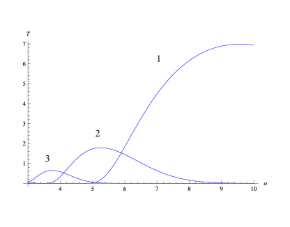
Figure 2: Transition temperature to the unconventional FISDW phases (measured in Kelvin) is calculated by means of Eq.(35) as a function of angle $\alpha$ (measured in degrees) and is given by a maximum value of three curves. Numbers 1,2,3 correspond to the values of integer $n$ for the quantized FISDW wave vector in Eq.(28). The calculations are made for $H=350\ T$ and the following realistic values of the physical parameters in the (TMTSF)₂PF₆: $\omega_{c}(\pi/2)/H=0.85\ K/T$ and $H_{0}\simeq 185\ T$.

Then, from Eq.(34), it directly follows that transition temperature to the different FISDW phases (28) with the logarithmic accuracy can be expressed as

$$T_{c}=\omega_{c}(\alpha)\ \exp\biggl{(}-\frac{\ln(H/H_{0})}{\max_{n}\biggl{\{}J^{2}_{n}[4t_{H}/\omega_{c}(\alpha)]\biggl{\}}}\bigg{)},\ H>H_{0},$$ (35)

where we have to take maximum of $T_{c}$ with respect to the integer $n$ to find a ground FISDW state (see Fig.2). As directly follows from Eq.(35), the physical meaning of the novel FISDW phases is different from that of standard ones [5-15]. First of all, in Eq.(35), we have unusual ”anti-nesting” term and related parameter $t_{H}\sim H$. Since $\omega_{c}(\alpha)$ is also proportional to $H$, the positions of the different FISDW phases, given by Eq.(35), do not depend on a strength of a magnetic field, in contrast to the standard case [1-6,7-15]. In addition, the following asymptotic property of the Bessel functions for $z\gg 1$ [18],

$$J_{n}(z)\approx\sqrt{\frac{2}{\pi z}}\cos\biggl{(}z-\frac{n\pi}{2}-\frac{\pi}{4}\biggl{)}$$ (36)

shows that the positions of the different FISDW phases at large values of integer $n$ in Eq.(28) are periodic with variable $1/\sin\alpha$.

In conclusion, let us discuss the possible applications of our theory to real Q1D conductors from the chemical family (TMTSF)₂X. We recall that, in Ref.[16], we have suggested novel effect, where SDW state is destroyed by some unusual ”anti-nesting” term. It appears due to the Pauli spin-splitting effects [see the second ”anti-nesting” term in Eq.(8)]. The theory [16] was elaborated for a magnetic field parallel to the conducting axis, ${\bf H}\parallel{\bf a}$ (i.e., for $\alpha=0$ in our case). As directly seen from Eq.(21), for any $H\neq 0$ and $\alpha\neq 0$ the FISDW phases are ground states at $T=0$. Therefore, for the analysis of the FISDW phases we always have to make use of our Eq.(21), which is more general than that used in the previous theories of the FISDW phases [5,6,8-15]. Below, we discuss where our final analytical Eq.(35) is literally applicable to describe novel FISDW phases suggested in the Letter. As an example, let us consider (TMTSF)₂PF₆ conductor. First, the magnetic field has to be stronger than the value of $H_{0}$, which is estimated as $H_{0}=185\ T$ (see Ref.[16]). Note that such high magnetic fields are now available (see, for example, Refs.[19,20]). Second, angle $\alpha$ has to be not very small in order inequality (22) to be fulfilled. If we estimate the value of $t^{\prime}_{b}\approx 5\ K$ from the expression $t^{\prime}_{b}=t^{2}_{b}/(2\sqrt{2}t_{a})$, then we obtain from Eq.(22) that $\alpha\geq 6^{0}$. It is possible to make sure that the inequality (31) is also fulfilled under the above mentioned conditions. Note that above we have estimated the values of a magnetic field, where the novel FISDW phases will appear, nevertheless our Eq.(21) predicts some changes in the known cascades of the FISDW phases. Hopefully, they will be studied by using numerical methods in the future.

We are thankful to N.N. Bagmet (Lebed) for useful discussions.

^∗Also at: L.D. Landau Institute for Theoretical Physics, RAS, 2 Kosygina Street, Moscow 117334, Russia.

References

- (1) See, for recent reviews, The Physics of Organic Superconductors and Conductors, edited by A.G. Lebed (Springer, Berlin, 2008).
- (2) T. Ishiguro, K. Yamaji, and G. Saito, Organic Superconductors, 2nd edn. (Springer, Berlin, 1998).
- (3) P.M. Chaikin, Mu-Yong Choi, J.F. Kwak, J.S. Brooks, K.P. Martin, M.J. Naughton, E.M. Engler, and R.L. Greene, Phys. Rev. Lett. 51, 2333 (1983).
- (4) M. Ribault, D. Jerome, J. Tuchendler, C. Weyl, and K. Bechgaard, J. Phys. (Paris) Lett. 44, L-953 (1983).
- (5) L.P. Gor’kov and A.G. Lebed, J. Phys. (Paris) Lett. 45, L-433 (1984).
- (6) M. Heritier, G. Montambaux, and P. Lederer, J. Phys. (Paris) Lett. 45, L-943 (1984).
- (7) K. Yamaji, J. Phys. Soc. Jpn. 51, 2878 (1982).
- (8) P.M. Chaikin, Phys. Rev. B 31, 4770 (1985).
- (9) A.G. Lebed, Sov. Phys. JETP, 62, 595 (1985) [Zh. Eksp. Teor. Fiz. 89, 1034 (1985)].
- (10) G. Montambaux, M. Heritier, and P. Lederer, Phys. Rev. Lett., 55, 2078 (1985).
- (11) K. Maki, Phys. Rev. B 33, 4826 (1986).
- (12) A.G. Lebed, Phys. Rev. Lett. 88, 177001 (2002).
- (13) D. Poilblanc, G. Montambaux, M. Heritier et al., Phys Rev. Lett. 58, 270 (1987).
- (14) V.M. Yakovenko, Phys. Rev. B 43, 11353 (1991).
- (15) K. Yamaji, Synth. Met. 13, 29 (1986).
- (16) A.G. Lebed, Phys. Rev. B 97, 220503(R) (2018).
- (17) A.A. Abrikosov, L.P. Gor’kov, and I.E. Dzyaloshinskii, Methods of Quantum Field Theory in Statistical Mechanics (Dover, New York, 1963).
- (18) I.S. Gradshteyn and I.M. Ryzhik, Table of Integrals, Series, and Products (6-th edition, Academic Press, London, United Kingdom, 2000).
- (19) A.S. Dzurak, B.E. Kane, R.G. Clark, N.E. Lumpkin, J. O’Brien, G.R. Facer, R.P. Starrett, A. Skougarevsky, H. Nakagawa, N. Miura, Y. Enomoto, D.G. Rickel, J.D. Goettee, L.J. Campbell, C.M. Fowler, C. Mielke, J.C. King, W.D. Zerwekh, A.I. Bykov, O.M. Tatsenko, V.V. Platonov, E.E. Mitchell, J. Hermann, and K.-H. Muller, Phys. Rev. B 57, R14084 (1998).
- (20) T. Sekitani, N. Miura, S. Ikeda, Y.H. Matsuda, and Y. Shiohara, Physica B 346-347, 319 (2004).