On beryllium-10 production in gaseous protoplanetary disks and implications on the astrophysical setting of refractory inclusions

Calcium-Aluminum-rich Inclusions (CAIs), the oldest known solids of the solar system, show evidence for the past presence of short-lived radionuclide beryllium-10, which was likely produced by spallation during protosolar flares. While such ¹⁰Be production has hitherto been modeled at the inner edge of the protoplanetary disk, I calculate here that spallation at the disk surface may reproduce the measured ¹⁰Be/⁹Be ratios at larger heliocentric distances. Beryllium-10 production in the gas prior to CAI formation would dominate that in the solid. Interestingly, provided the Sun’s proton to X-ray output ratio does not decrease strongly, ¹⁰Be/⁹Be at the CAI condensation front would increase with time, explaining the reduced values in a (presumably early) generation of CAIs with nucleosynthetic anomalies. CAIs thus need not have formed very close to the Sun and may have condensed at 0.1-1 AU where sufficiently high temperatures originally prevailed.

1 Introduction

Primitive meteorites, or chondrites, are conglomerates of solids which formed and accreted in the solar protoplanetary disk. Among those, the oldest are the refractory inclusions, comprising Calcium-Aluminium-rich Inclusions (CAIs) and Amoeboid Olivine Aggregates (AOA) (e.g. MacPherson 2014; Krot et al. 2004). Thermodynamic calculations predict that CAIs should be the first condensates in a cooling gas of solar composition (Grossman 2010; Davis and Richter 2014). Since the required temperatures would be in the range 1500-2000 K (Wooden et al. 2007), it is widely assumed that refractory inclusions formed close to the Sun, but precisely how close and in what astrophysical setting remains unclear (Wood 2004; Jacquet 2014).

An important clue in this respect may be provided by beryllium-10, a short-lived radio-isotope decaying into boron-10 with a half-life of 1.5 Ma, and which, unlike other known extinct radionuclides such as aluminum-26, is not produced by stellar nucleosynthesis but may be formed through spallation by energetic particles (Davis and McKeegan 2014; Lugaro et al. 2018). Indeed, since the original discovery by McKeegan et al. (2000), all CAIs with analytically suitable Be/B have shown ¹⁰B/¹¹B excesses correlated therewith. The slopes of the resulting isochrons translate into initial (i.e. upon the last equilibration) ¹⁰Be/⁹Be ratios averaging $\sim 6\times 10^{-4}$ in CV chondrite (type A and B) CAIs (Davis and McKeegan 2014), with less than a factor of two spread. Yet systematically lower values around $3\times 10^{-4}$ and $5\times 10^{-4}$ have been found for two CV chondrite FUN CAIs (”Fractionated and Unknown Nuclear effects”; MacPherson et al. (2003); Wielandt et al. (2012)) and platy hibonite crystals (PLAC) in CM chondrites (Liu et al. 2009, 2010), respectively, and, conversely, values up to $10^{-2}$ have been found for Isheyevo CAI 411 (Gounelle et al. 2013) and more recently, fine-grained group II CV chondrite CAIs (Sossi et al. 2017). The overall spread, along with correlated ⁵⁰V excesses (also ascribed to spallation) in the latter objects (Sossi et al. 2017), is difficult to reconcile with simple ¹⁰Be inheritance from the (galactic cosmic ray-irradiated) protosolar cloud (Desch et al. 2004), which should be largely homogeneous, and argues in favor of local production in the disk following flares from the young Sun (Gounelle et al. 2001, 2006, 2013; Sossi et al. 2017), such as those manifested in X-rays by present-day protostars (e.g. Feigelson et al. 2002; Wolk et al. 2005; Preibisch et al. 2005; Telleschi et al. 2007; Güdel et al. 2007; Bustamante et al. 2016) or evidence for enhanced ionization in some protostellar envelopes (Ceccarellietal2014; Favreetal2017; Favreetal2018).

Since the energetic protons would not penetrate further than $\sim 690\>\mathrm{kg/m^{2}}$ (Umebayashi and Nakano 1981) in the gas, Sossi et al. (2017) suggested that CAIs spent a few thousand orbits at the inner edge of the protoplanetary disk, similar to earlier studies which had adopted the framework of the X-wind scenario (Lee et al. 1998; Shu et al. 2001; Gounelle et al. 2001). However, among the objections to the latter discussed by Desch et al. (2010), a general issue is that CAI-forming temperatures would be expected significantly further outward (0.1-1 AU), because of local dissipation of turbulence. If nonetheless CAIs all went somehow through this narrow region, escaped accretion to the Sun or ejection from the solar system they would be essentially ”lucky” foreign material in the chondrites which incorporated them. Yet CAIs are present in carbonaceous chondrites at about the abundances predicted by in situ condensation (Jacquet et al. 2012). Also, although (non-CI) carbonaceous chondrites are enriched in refractory elements relative to CI chondrites, this cannot be ascribed to simple CAI addition to CAI-free CI chondritic material for should the CAIs be mentally subtracted, these chondrites would have subsolar refractory element abundances (Hezel et al. 2008), not even considering those CAIs that were converted into chondrules (Misawa and Nakamura 1988; Jones and Schilk 2009; Metzler and Pack 2016; Ebert and Bischoff 2016; Jacquet and Marrocchi 2017; Marrocchi et al. 2018). Isotopic systematics for elements of different volatilities also indicate a need for a non-refractory isotopically CAI-like component in chondrites (e.g. Nanneetal2019). So there is evidence for a genetic relationship between CAIs and (part of) their host carbonaceous chondrites which argues against an origin at the disk inner edge, whose contribution to distant chondritic matter would likely be minor.

However, the inner edge of the disk is not the only region where CAIs or their precursors could have been exposed to energetic solar protons. CAIs floating further out in the disk would at times reach the upper layers of the disk. While such excursions may individually incur modest proton fluences, their cumulative contributions might explain the total ¹⁰Be evidenced in CAIs. Moreover, prior to CAI condensation, the gas exposed at the surface of the disk may also undergo spallation and pass on the then-produced ¹⁰Be to the later-formed condensates. The purpose of this paper is to analytically calculate the amount of beryllium-10 produced by such channels and thence evaluate the viability of having CAIs form at 0.1-1 AU from the young Sun against their irradiation record. Figure 1 provides a sketch of the overall scenario and setting. After several generalities in Section 2, I will express the ¹⁰Be/⁹Be ratio in the disk and free-floating solid CAIs in Section 3. I then discuss the numerical evaluations thereof and their implications in Section 4 before concluding in Section 5.

2 Prolegomena

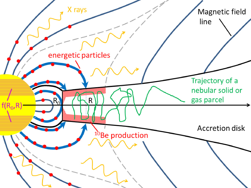
Figure 1: Sketch of the scenario of ¹⁰Be production developed in this paper. Solar cosmic rays cause spallation reactions in the upper layers of the disk, in the gas and/or condensates, within a region (outlined by a dashed separatrix) where magnetic field lines originating from the proto-Sun and its outskirts hit the disk. The field and particle emission geometries are purely illustrative and do not detract the generality of the formalism.

2.1 Disk model

I consider a protoplanetary disk in a cylindrical coordinate system with heliocentric distance $R$. The inner regions can be described under the steady state approximation so long the evolution timescales of the system are long compared to their local viscous timescale

$$t_{\rm vis}\left(R\right) \equiv \frac{R^{2}}{\nu}$$ (1)

$$= 0.02\>\mathrm{Ma}\left(\frac{R}{0.5\>\rm UA}\right)^{1/2}\left(\frac{1500\>\rm K}{T}\right)\left(\frac{10^{-3}}{\alpha}\right),$$

where $\nu=\alpha c_{s}^{2}/\Omega_{K}$ is the effective turbulent viscosity, $\alpha$ the dimensionless turbulence parameter (e.g. Jacquet 2013), $c_{s}=\sqrt{k_{B}T/m}$ the isothermal sound speed with $k_{B}$ the Boltzmann constant, $T$ the temperature and $m=3.9\times 10^{-27}\>\rm kg$ the mean molecular mass, and $\Omega_{K}$ the Keplerian angular velocity. Since $t_{\rm vis}(R)$ is also much shorter than the half-life of ¹⁰Be, I will neglect its decay during the CAI formation epoch. This is consistent with the short timescales (no more than a few hundreds of millenia) of CAI formation and (isotopically resetting) re-heating events (e.g. MacPherson 2014), which should have ended after the last production of ¹⁰Be so as to account for the isochron behavior of the Be-B system in each CAI (that is, with ¹⁰B excesses scaling with Be rather than the target nuclides leading to its parent; see next subsection).

If infall from the parental cloud can be neglected in the inner region, the disk mass accretion rate $\dot{M}=-2\pi R\Sigma u_{R}$ (with $\Sigma$ the disk surface density and $u_{R}$ the net, turbulence-averaged, gas radial velocity) is uniform and obeys:

$$\dot{M}\left(1-\sqrt{\frac{R_{0}}{R}}\right)=3\pi\Sigma\nu,$$ (2)

or, equivalently,

$$u_{R}=-\frac{3\nu}{2R\left(1-\sqrt{R_{0}/R}\right)},$$ (3)

where we have assumed that the stress vanishes at the disk inner edge $R_{0}$ (e.g. Balbus and Hawley 1998). When calculating ¹⁰Be/⁹Be in later sections, I shall show expressions for a general $\dot{M}(R)$ before specializing to the case of uniform mass accretion rate. Appendix A explores the corrections of infall to equation (2).

If I inject the temperature due to viscous dissipation of turbulence (e.g. appendix A of Jacquet et al. (2012)) in equation (2), I obtain:

$$T = \left(\frac{3\kappa m\dot{M}^{2}\left(1-\sqrt{R_{0}/R}\right)^{2}\Omega_{K}^{3}}{128\pi^{2}\sigma_{SB}k_{B}\alpha}\right)^{1/5}$$ (4)

$$= 1200\>\mathrm{K}\left(\frac{\kappa}{10^{-2}\>\rm m^{2}/kg}\right)^{1/5}\left(\frac{10^{-3}}{\alpha}\right)^{1/5}\left(1-\sqrt{\frac{R_{0}}{R}}\right)^{2/5}$$

$$\left(\frac{0.5\>\rm AU}{R}\right)^{9/10}\left(\frac{\dot{M}}{10^{-7}\>\rm M_{\odot}/a}\right)^{2/5}$$

with $\kappa$ the specific Rosseland mean opacity and $\sigma_{SB}$ the Stefan-Boltzmann constant. This confirms that CAI-forming temperatures may be reached at a fraction of an AU for $\dot{M}\gtrsim 10^{-7}\>\rm M_{\odot}/a$.

2.2 ¹⁰Be production rate

The local production rate of ¹⁰Be by spallation normalized to ⁹Be may be written as (e.g. Sossi et al. 2017):

$$\left(\frac{\overset{\bullet}{{}^{10}\rm Be}}{{}^{9}\rm Be}\right)_{\rm tg}=\int_{0}^{+\infty}\mathrm{d}E\sigma_{ki}(E)\left(\frac{k}{\rm Be}\right)_{\rm tg}\int\mathrm{d}\Omega I(i,E,\Omega)$$ (5)

with $\sigma_{ki}$ the ¹⁰Be production cross section for target (tg) nuclide $k$ and cosmic ray species $i$ (with energy per nucleon $E$) and $I(i,E,\Omega)$ the corresponding (orientation-dependent) monoenergetic cosmic ray specific intensity (defined by number and not energy, as in Gounelle et al. 2001). Here and throughout, all isotopic or elemental ratios are atomic and the Einstein convention for summation over the repeated indices $k$ and $i$ is adopted. I assume that the incoming cosmic rays have a solar composition (but see Mewaldt et al. (2007) for details on contemporaneous solar energetic particles), with e.g. ⁴He/H=0.1, and obey a power law $\propto E^{-p}$ for $E\geq E_{\rm 10}\equiv 10\>\rm MeV$ upon arrival on the disk. I will ignore the contribution of secondary neutrons, despite their comparable cross sections (e.g. LeyaMasarik2009) and larger attenuation columns. This is because a dilute medium such as the surface of the disk will let free decay thwart significant accumulation of neutron flux (Umebayashi and Nakano 1981). However, based on this latter work, this is only marginally true (see equation (C) in appendix C), so the production rates given here should be strictly viewed as a lower bounds.

In the following sections, we will be interested in the density ($\rho$)-weighted vertical average of the production rate at a given heliocentric distance:

$$\left\langle\left(\frac{\overset{\bullet}{{}^{10}\rm Be}}{{}^{9}\rm Be}\right)_{\rm tg}\right\rangle_{\rho}\equiv\frac{1}{\Sigma}\int_{0}^{\Sigma}\mathrm{d}\Sigma^{\prime}\left(\frac{\overset{\bullet}{{}^{10}\rm Be}}{{}^{9}\rm Be}\right)_{\rm tg}\approx\frac{2}{\Sigma}\int_{0}^{+\infty}\mathrm{d}\Sigma^{\prime}\left(\frac{\overset{\bullet}{{}^{10}\rm Be}}{{}^{9}\rm Be}\right)_{\rm tg,+}$$ (6)

where $\Sigma^{\prime}$ is the column density integrated vertically from the upper surface and the $+$ subscript in the final equality denotes restriction to cosmic rays from the upper side, assuming $\Sigma$ is much larger than the attenuation column $\Sigma_{p,i}(E)$ of the cosmic rays, defined here as:

$$\Sigma_{p,i}(E)\equiv\frac{1}{I_{+}(i,E,\Omega;0)}\int_{0}^{+\infty}\mathrm{d}\Sigma^{\prime\prime}I_{+}(i,E,\Omega;\Sigma^{\prime\prime})$$ (7)

where $\Sigma^{\prime\prime}$ is the actually traversed column density. If I envision a cosmic ray beam (with the particles gyrating along a magnetic field line) penetrating the disk with a grazing angle $\phi$ and ignore secondary particles, $\Sigma^{\prime\prime}=\Sigma^{\prime}/(\mu\mathrm{sin}\phi)$ with $\mu$ the cosine of the pitch angle of the cosmic ray with respect to the magnetic field line (Padovani et al. 2018). I thus obtain:

$$\left\langle\left(\frac{\overset{\bullet}{{}^{10}\rm Be}}{{}^{9}\rm Be}\right)_{\rm tg}\right\rangle_{\rho}=\frac{2}{\Sigma}\int_{0}^{+\infty}\mathrm{d}E\sigma_{ki}(E)\Sigma_{p,i}(E)\left(\frac{k}{\rm Be}\right)_{\rm tg}\left(\frac{i}{\rm H}\right)_{\rm CR}\frac{\mathrm{d}\mathbf{F}_{H}}{\mathrm{d}E}\cdot\mathbf{n}$$ (8)

where $\mathbf{n}$ is the downward-directed unit vector normal to the disk surface and $\mathrm{d}\mathbf{F}_{H}/\mathrm{d}E$ the incoming differential proton number vector flux. If I scale the latter to the incoming $>$ 10 MeV/nucleon energy vector flux $\mathbf{F}_{10}$ and extract O as a proxy for all ¹⁰Be-producing target nuclides, equation (8) can be further manipulated to finally yield:

$$\left\langle\left(\frac{\overset{\bullet}{{}^{10}\rm Be}}{{}^{9}\rm Be}\right)_{\rm tg}\right\rangle_{\rho}=\frac{K_{p}L_{10}}{2\pi R\Sigma}\left(\frac{\rm O}{\rm Be}\right)_{\rm tg}\frac{\partial f(R_{0},R)}{\partial R}$$ (9)

with

$$K_{p}\equiv\left(p-2\right)E_{10}^{p-2}\left(\frac{k}{\rm O}\right)_{\rm tg}\left(\frac{i}{\rm H}\right)_{\rm CR}\int_{0}^{+\infty}\mathrm{d}E\sigma_{ki}(E)\Sigma_{p,i}(E)E^{-p},$$ (10)

which is plotted in Fig. 2 (see Appendix B for further details on its calculation and data sources). $f(a,b)$ is the fraction of the total $>$10 MeV/nucleon energy luminosity $L_{10}$ which reaches the disk between heliocentric distances $a$ and $b$. The latter depends on the geometry of energetic particle emission and the magnetic field configuration around the young Sun, which are largely unknown (protosolar corona, star-disk fields or disk fields; Feigelson et al. (2002); DonatiLangstreet2009). For reference, in the case of a geometrically flared disk, an isotropic point source with straight trajectories would yield $f(R_{0},R)=H_{\rm spall}/R$ with $H_{\rm spall}$ the height of the spallation layer above the midplane (see Appendix C for an estimate). For illustration in the plots of the next section, I will use a form of $f$ assuming that the outgoing energy flux density of the energetic particles is uniform over the Sun-centered sphere of radius $R_{0}$ and that the magnetic field is approximately dipolar (with a magnetic moment along the rotation axis of the disk) for fieldlines interior to a maximum irradiation distance $R_{\rm max}$. This yields:

$$f(R_{0},R)=\mathrm{max}\left(\sqrt{1-\frac{R_{0}}{R}},\sqrt{1-\frac{R_{0}}{R_{\rm max}}}\right).$$

However, in the main text, I will keep general expressions as functions of $f$. This parameterization of our ignorance will turn out to be quite handy in the calculation.

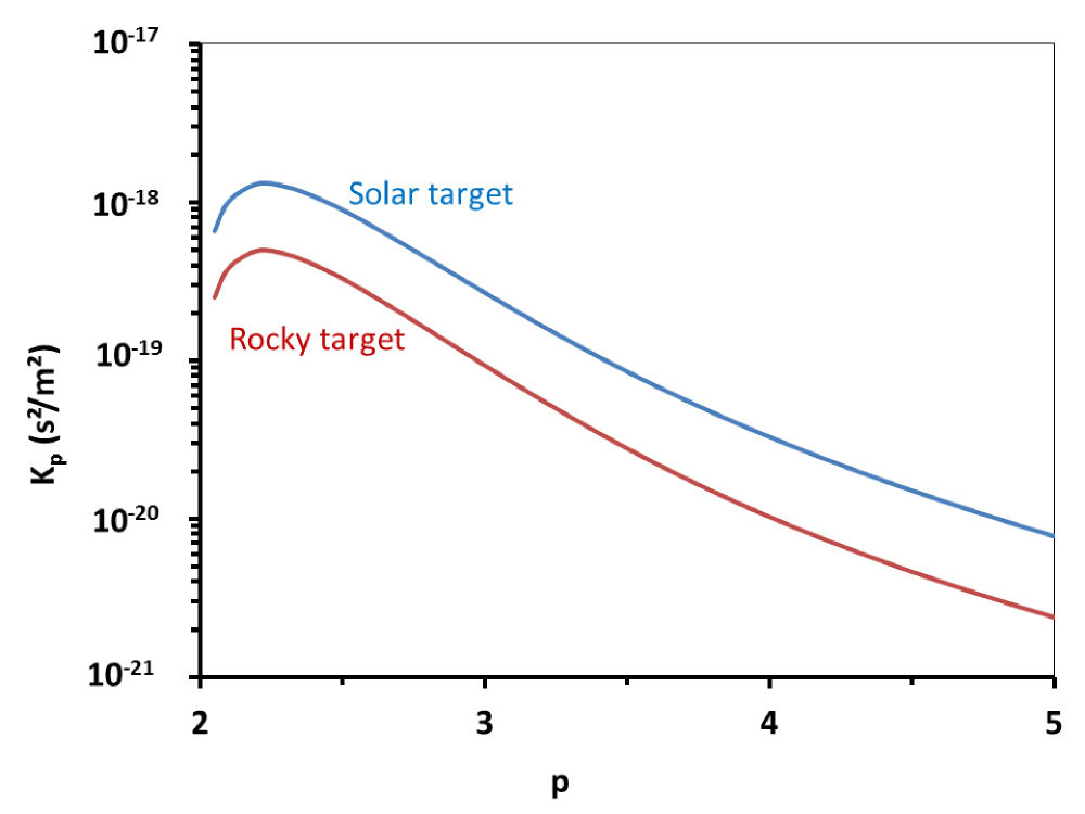
Figure 2: Plot of $K_{p}$ as a function of the power law exponent of the incoming cosmic ray energy distribution, for a solar (without possible implantation contributions) and a rocky target (see subsections 3.1 and 3.2, respectively).

A means of comparison with previous models invoking irradiation of bare solids (e.g. Lee et al. 1998; Gounelle et al. 2006; Sossi et al. 2017) is to divide the rate given by equation (9) by that in a target of the same composition exposed to the same unattenuated proton flux. Assuming isotropic distribution of cosmic rays (in each half-space along the field line), this gives:

$$\frac{\overset{\bullet}{{}^{10}\rm Be}}{\overset{\bullet}{{}^{10}\rm Be}_{\rm bare}}=\frac{\langle\Sigma_{p}(E)\rangle_{\sigma E^{-p}}\mathrm{sin}\phi}{\Sigma}$$ (12)

with

$$\langle\Sigma_{p}(E)\rangle_{\sigma E^{-p}}\equiv\left(\frac{k}{\rm O}\right)_{\rm tg}\left(\frac{i}{\rm H}\right)_{\rm CR}\int_{0}^{+\infty}\mathrm{d}E\sigma_{ki}(E)\Sigma_{p,i}(E)E^{-p}$$

$$\Bigg{/}\left[\left(\frac{k}{\rm O}\right)_{\rm tg}\left(\frac{i}{\rm H}\right)_{\rm CR}\int_{0}^{+\infty}\mathrm{d}E\sigma_{ki}(E)E^{-p}\right],$$ (13)

which (for a refractory target) is 90 kg/m² for p = 2.5 typical of gradual flares favored by Gounelle et al. (2013) and Sossi et al. (2017), and 5 kg/m² for p = 4 commensurate with impulsive flares (with subdominant fluences in the present-day Sun; Desai and Giacalone 2016). Obviously, for $\Sigma\gg 10^{4}\>\rm kg/m^{2}$ (the Minimum Mass Solar Nebula at 1 AU; Hayashi1981) this calls for (intermittent) irradiation timescales $2\pm 1$ orders of magnitude above the centuries calculated by Sossi et al. (2017). As alluded in the introduction, the transport timescale $t_{\rm vis}$ may however provide the correct order of magnitude. The following section undertakes to calculate more precisely the net ¹⁰Be abundances produced in gas and solids and during radial transport.

3 ¹⁰Be abundances

3.1 Bulk ¹⁰Be/⁹Be in the disk

In this subsection, I calculate the average ¹⁰Be/⁹Be of the disk as a function of heliocentric distance, irrespective of its (temperature-dependent) physical state (condensation fraction) to which spallation reactions are insensitive. I assume solar abundances throughout the inner disk owing to tight coupling of the condensates with the gas (e.g. Jacquet et al. 2012).

A steady-state gradient of ¹⁰Be/⁹Be should arise in the disk because production of ¹⁰Be is balanced by loss to the Sun by accretion. The transport equation reads:

$$\frac{1}{R}\frac{\partial}{\partial R}\Bigg{[}R\Bigg{(}\Sigma u_{R}c_{\rm Be}\left(\frac{{}^{10}\rm Be}{{}^{9}\rm Be}\right)_{\rm disk}-D_{R}\Sigma\frac{\partial}{\partial R}\left(c_{\rm Be}\left(\frac{{}^{10}\rm Be}{{}^{9}\mathrm{Be}}\right)_{\rm disk}\right)\Bigg{)}\Bigg{]}$$

$$=\Sigma c_{\rm Be}\left\langle\left(\frac{\overset{\bullet}{{}^{10}\rm Be}}{{}^{9}\rm Be}\right)_{\rm disk}\right\rangle_{\rho}=\frac{K_{p,\rm disk}L_{10}c_{\rm O}}{2\pi R}\frac{\partial f(R_{0},R)}{\partial R}$$ (14)

with $c_{\rm Be,O}$ the Be, O concentration in number per unit mass of solar gas and $D_{R}$ the turbulent diffusion coefficient. The $K_{p,\rm disk}$ factor here includes contributions from $k=^{12}$C, ¹⁶O and ¹⁴N (even though the last one is unimportant, with N/O=0.14, compared to C/O=0.5; Lodders 2003) and $i$=¹H, ⁴He. In addition, it includes contributions from indirect reactions (Desch et al. 2004), that is those where the heavy nuclei originate from the cosmic rays instead of the target, since, although the hereby produced ¹⁰Be will retain the momentum of the incoming particles, it should be stopped further downstream in the disk. Since Galilean invariance mandates $\sigma_{ik}=\sigma_{ki}$, this amounts to multiplying each ”direct” reaction contribution in the right-hand-side of equation (10) by $1+\left[(k/i)_{\rm CR}/(k/i)_{\rm disk}\right]\Sigma_{p,k}(E)/\Sigma_{p,i}(E)=1+A_{k}/Z_{k}^{2}$ where the second expression uses the assumption that the disk has a (solar) composition, identical to the cosmic rays’ (see also Appendix B). $K_{p,\rm disk}$ is plotted as the ”solar target” curve in Fig. 2

Another ”indirect” contribution would be solar wind implantation of ¹⁰Be produced on the protoSun (Bricker and Caffee 2010). Although Bricker and Caffee (2010) originally envisioned implantation on bare solids, one can equally envision implantation on the gas disk surface (followed by vertical mixing); this would amount to adding $(L_{{}^{10}\rm Be}/2\pi R)\partial f_{\rm SW}/\partial R$ to the right-hand-side of equation (3.1) with $L_{{}^{10}\rm Be}$ the young Sun’s ¹⁰Be (number) production rate and $f_{\rm SW}$ the counterpart of $f$. This would amount to an effective increase of $K_{p,\rm disk}$ of $(\mathrm{d}f_{\rm SW}/\mathrm{d}f)L_{{}^{10}\rm Be}/(L_{10}c_{\rm O})$. If I set $\mathrm{d}f_{\rm SW}/\mathrm{d}f(L_{{}^{10}\rm Be}/L_{10})$ equal to the present-day ratio of long-term average 1 AU ¹⁰Be (Nishiizumi and Caffee 2001) and $>$10 MeV proton (Reedy 1996) energy omnidirectional fluxes, this evaluates to $6\times 10^{-20}\>\rm s^{2}/m^{2}$. From Fig. 2, at face value, solar wind implantation thus appears negligible compared to local (in-disk) spallation (except for steep $p\gtrsim 4$) but since we do not really know how ¹⁰Be production on the Sun must be extrapolated to its very active early times, the nominal one order-of-magnitude deficit may not warrant definitive conclusions yet.

Returning to equation (3.1), the requirement that ¹⁰Be/⁹Be vanishes at infinity leads to the following first integration:

$$\left(\frac{\partial}{\partial R}-\frac{u_{R}}{D_{R}}\right)\left(\frac{{}^{10}\rm Be}{{}^{9}\rm Be}\right)_{\rm disk}=\frac{K_{p,\rm disk}L_{10}}{2\pi R\Sigma D_{R}}\left(\frac{\rm O}{\rm Be}\right)_{\rm disk}f(R,+\infty)$$ (15)

Provided the radial Schmidt number Sc${}_{R}\equiv\nu/D_{R}$ has a finite lower bound, the requirement that ¹⁰Be/⁹Be does not diverge at the inner edge of the disk (since $u_{R}/D_{R}$ would not be integrable there from equation (3)) leads to the unique solution:

$$\left(\frac{{}^{10}\rm Be}{{}^{9}\rm Be}\right)_{\rm disk} = K_{p,\rm disk}L_{10}\left(\frac{\rm O}{\rm Be}\right)_{\rm disk}\Bigg{[}\frac{f(R,+\infty)}{\dot{M}}$$ (16)

$$-\int_{R_{0}}^{R}\mathrm{exp}\left(\int_{R^{\prime}}^{R}\frac{u_{R}}{D_{R}}\mathrm{d}R^{\prime\prime}\right)\frac{\partial}{\partial R}\left(\frac{f(R^{\prime},+\infty)}{\dot{M}}\right)\mathrm{d}R^{\prime}\Bigg{]}$$

$$= \frac{K_{p,\rm disk}L_{10}}{\dot{M}}\left(\frac{\rm O}{\rm Be}\right)_{\rm disk}f_{\rm eff},$$

where the second equality assumes uniform $\dot{M}$ and Sc_R, with

$$f_{\rm eff}\equiv f(R,+\infty)+\int_{R_{0}}^{R}\left(\frac{R^{\prime 1/2}-R_{0}^{1/2}}{R^{1/2}-R_{0}^{1/2}}\right)^{3\mathrm{Sc}_{R}}\frac{\partial f(R_{0},R^{\prime})}{\partial R}\mathrm{d}R^{\prime},$$ (17)

which is plotted in Fig. 3.

Interestingly, the result is weakly sensitive to the details of the protoplanetary disk (e.g. turbulence level etc.) with the reference to heliocentric distance being only implicit in $f_{\rm eff}$. This is because the approximate $\propto R^{-2}$ decrease of the flux density is essentially compensated by the $R^{2}$ factor in the radial transport timescale $t_{\rm vis}$. The above expression can be interpreted as a sum of contributions advected from outer regions (see next subsection, in particular equation (19)) and contributions diffused back outward. ¹⁰Be/⁹Be decreases monotonically outward, falling off roughly as $R^{-3\mathrm{Sc}_{R}/2}$ outside the irradiated region, conform to the equilibrium gradient of a passive scalar (Clarke and Pringle 1988; Jacquet and Robert 2013). In the limit Sc${}_{R}\rightarrow 0$, it converges pointwise toward the inner edge value $f(R_{0},+\infty)$ and a flat profile, but Sc_R is probably of order unity in MHD turbulence (Johansen et al. 2006), not to mention the possibility of laminar wind-driven accretion (and thus even higher Sc_R) further out (e.g. Bai 2016). So contrary to earlier statements (Gounelle et al. 2013; Koopetal2018Ne), ¹⁰Be production in the gas would entail no spatial uniformity of the ¹⁰Be/⁹Be ratio.

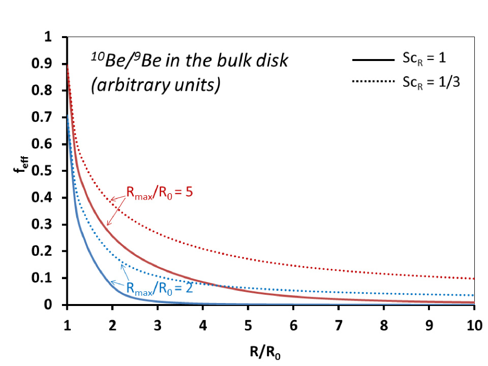
Figure 3: Plot of $f_{\rm eff}$ (equation (17)) as a function of heliocentric distances for two values of $R_{\rm max}$ for my toy parameterization of the particle flux distribution (see end of section 2.2) and two values of the radial Schmidt number, with the lower one (higher relative diffusivity) in dotted lines. $f_{\rm eff}$ is proportional to the ¹⁰Be/⁹Be ratio (whose absolute magnitude is discussed at equation (4.1)) in the bulk (gas+solids) disk for given mass accretion rate and proton output and energy distributions.

3.2 In situ ¹⁰Be production in free-floating solids

I now consider a (sub-)millimeter rocky solid, say a CAI, formed (or more precisely, whose beryllium last equilibrated with the gas) at an heliocentric distance $R_{1}$. It will certainly inherit the ¹⁰Be/⁹Be ratio of the local reservoir calculated above, but it should also acquire additional ¹⁰Be so long it wanders through the irradiated region of the disk. The purpose of this subsection is to estimate this contribution.

Since the inner disk (where irradiation may occur) is dense, I assume the solid to be tightly coupled to the gas (that is, a gas-grain decoupling parameter $S\ll 1$; Jacquet et al. 2012; this is consistent with the lack of bulk chemical fractionation assumed previously). It is also small enough for the thin target approximation (e.g. Sossi et al. 2017) to apply, that is, for equation (5) to apply at the scale of the whole particle as a function of the local (outside) monoenergetic intensities. Since the radial transport timescale $t_{\rm vis}$ is much longer than the vertical transport timescale $H^{2}/\nu$ with $H=c_{s}/\Omega_{K}$ the pressure scale height, I can use the average rate of ¹⁰Be production given by equation (9). That is, I view the random vertical motion of the solids due to turbulence as an ergodic process (see e.g. Fig. 8 in Ciesla 2010) and identify the time average of this rate for a given solid to the instantaneous average over the long-term probability distribution of same-size solids, which here follows the distribution of the gas (but see appendix C for the case of finite settling). For this refractory target, the sum on the right-hand-side of equation (10) is essentially restricted to $k$=O and $i$=¹H, ⁴He (with no ”indirect reaction” contribution). This corresponds to the ”rocky target” curve in Fig. 2.

As a result of the turbulent diffusion superimposed on advection by the gas mean velocity, the radial motion of an individual solid has a stochastic character. I will be content to set the ”typical timescale” spent crossing a radial bin of width $\Delta R\ll R$ to $|\Delta R/u_{R}|$. Indeed, even when the flow is opposite to the transport envisioned (as in this subsection), the fraction of a population of solids at $R$ at $t=0$ which has diffused upstream beyond that distance at time $t$ ($\sim\mathrm{erfc}\left((\Delta R-u_{R}t)/\sqrt{4D_{R}t}\right)/2$, with erfc the complementary error function), is maximum for $t=-\Delta R/u_{R}$. The total ¹⁰Be produced in the solid during transport between an heliocentric distance $R_{1}$ and its exit from the irradiated region is then given by:

$$\left(\frac{{}^{10}\rm Be}{{}^{9}\rm Be}\right)_{\rm CAI} = \int_{R_{1}}^{+\infty}\left\langle\left(\frac{\overset{\bullet}{{}^{10}\rm Be}}{{}^{9}\rm Be}\right)_{\rm tg}\right\rangle_{\rho}\frac{\mathrm{d}R}{|u_{R}|}$$ (19)

$$= K_{p,\rm CAI}L_{10}\left(\frac{\rm O}{\rm Be}\right)_{\rm CAI}\int_{R_{1}}^{+\infty}\frac{\partial f(R_{0},R)}{\partial R}\frac{\mathrm{d}R}{\dot{M}}$$

$$= \frac{K_{p,\rm CAI}L_{10}}{\dot{M}}\left(\frac{\rm O}{\rm Be}\right)_{\rm CAI}f(R_{1},+\infty)$$

where the last equality assumes a uniform $\dot{M}(R)$. $f(R,+\infty)$ is plotted in Fig. 4. Unlike the inherited disk value (which benefitted from outward diffusion), nonzero values do not extend to source radii outside the irradiated region.

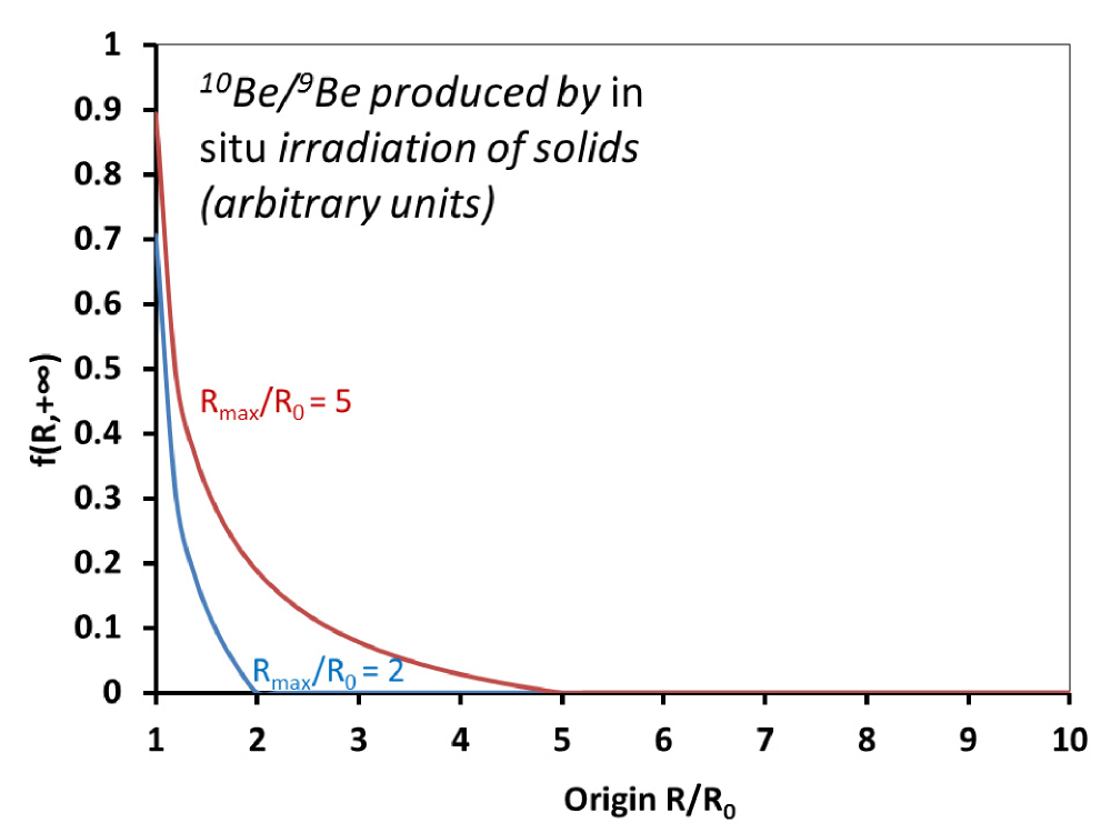
Figure 4: Plot of $f(R,+\infty)$ as a function of heliocentric distances for two values of $R_{\rm max}$ for my toy parameterization of the particle flux distribution (see end of section 2.2). This is proportional to the ¹⁰Be/⁹Be ratio produced by in situ irradiation of a refractory solid as a function of its heliocentric distance of origin.

4 Discussion

4.1 Magnitude of ¹⁰Be production

Provided a given CAI underwent isotopic equilibration after the last production of ¹⁰Be, the ¹⁰Be/⁹Be indicated by the slope of an internal isochron is the sum of that inherited from the disk gas and that produced in situ in the solid (equations (16) and (19), respectively), which may be written as:

$$\left(\frac{{}^{10}\rm Be}{{}^{9}\rm Be}\right)_{\rm final}=\frac{K_{p,\rm disk}L_{10}f_{\rm sum}}{\dot{M}}\left(\frac{\rm O}{\rm Be}\right)_{\rm disk}$$ (20)

with

$$f_{\rm sum}\equiv f(R_{1},+\infty)\left(1+\frac{K_{p,\rm CAI}\left(\mathrm{O}/\mathrm{Be}\right)_{\rm CAI}}{K_{p,\rm disk}\left(\mathrm{O}/\mathrm{Be}\right)_{\rm disk}}\right)$$

$$+\int_{R_{0}}^{R_{1}}\left(\frac{R^{\prime 1/2}-R_{0}^{1/2}}{R_{1}^{1/2}-R_{0}^{1/2}}\right)^{3\mathrm{Sc}_{R}}\frac{\partial f(R_{0},R)}{\partial R}\mathrm{d}R^{\prime}$$ (21)

The contribution of in situ production (the term with the ”‘CAI”’ subscripts in the above equation) is subdominant with respect to spallation in the solar gas (that is, $f_{\rm sum}\approx f_{\rm eff}(R_{1})$) since, not to mention the ignored incipient settling (see appendix C), (i) $K_{p,\rm disk}$ outweighs $K_{p,\rm CAI}$ by a factor of $\sim$3 (Fig. 2) as it includes additional production channels (e.g. target ¹²C, and indirect reactions) and (ii) Be, as a refractory element (half-condensation temperature of 1452 K according to Lodders (2003)), should be concentrated relative to O in a CAI with respect to the overall disk. Indeed Be concentrations typically are of order 0.1-1 ppm in the data of McKeegan et al. (2000); Gounelle et al. (2013), compared to the CI chondrite value of 25.2 ppb (the latter amounting to $\mathrm{O}/\mathrm{Be}=10^{7}\approx$ half the solar value; Palmeetal2014). Nevertheless, the fine-grained CAIs of Sossi et al. (2017) exhibit concentrations down to 6 ppb. So, at least for some Be-poor CAIs having spent a random walk in the irradiated region of the disk longer than the ”typical timescale” used in subsection 3.2, in situ production may not be entirely negligible. The deviation of the initial boron isotopic composition from solar in some CAIs, too large for an irradiated solar gas, may be a collateral effect of such a contribution (Liu et al. 2010; Gounelle et al. 2013); same for cosmogenic ³He and ²¹Ne excesses found by Koopetal2018Ne in the same type of inclusions. This indicates that, at least for some objects, heliocentric distance $R_{1}$ was inside the proton-irradiated region of the disk.

In order to numerically evaluate equation (20), I will, as previous authors (Lee et al. 1998; Gounelle et al. 2001; Sossi et al. 2017), use the X-ray luminosity $L_{X}$ as a proxy for $L_{10}$, since only the former can be measured from distant young stellar objects (although Ceccarellietal2014 estimated a proton output equivalent to $L_{10}\gtrsim 10^{27}$W, for $L_{X}<7\times 10^{24}$W, from the ionization level seen toward the single source OMC-2 FIR 4). Since their luminosities are higher than the most powerful flares of the contemporaneous Sun (e.g. Feigelson et al. 2002), solar flares are the least improper analogs in that calibration. Lee et al. (1998) derived a scaling $L_{10}=0.09L_{X}$ by ratioing the total proton and X-ray fluences of the impulsive flares of solar cycle 21 (peaking around 1980). However, while impulsive flares correlate best with X-ray outputs (Lee et al. 1998), gradual flares actually dominate the proton fluences at 1 AU (Desai and Giacalone 2016), whatever the ratio at the X point considered by Lee et al. (1998) may be. This warrants re-examination of the scaling between X rays and solar energetic particles (SEP) without restricting to impulsive flares. Emslie et al. (2012) evaluated the energy outputs of 38 solar eruptive events between 2002 and 2006. Those 21 with reported SEP outputs totaled a SEP output of $1.5\times 10^{25}$J (dominated by $>$10 MeV protons since the energy spectra is shallower below this; Mewaldt 2006) and $2.6\times 10^{24}$J in X-rays, hence a ratio of average $L_{10}/L_{X}\approx 6$ which I adopt as a normalizing value. Another relevant—if more indirectly for our purpose—dataset is the catalogue of 314 SEP events between 1984 and 2013 of Papaioannou et al. (2016). They represent a total $>$10 MeV proton 1 AU energy fluence of $5.1\times 10^{3}\>\rm J/m^{2}$ and total X ray fluence of $54\>\rm J/m^{2}$ hence $(L_{10}/L_{X})\partial f/\partial\mathrm{ln}R/\mathrm{sin}\phi\approx 23$ (which averages different geometries of the flare sources vis-à-vis the Earth) assuming isotropic distribution of SEP at 1 AU, suggestive of the same order of magnitude for $L_{10}/L_{X}$. Equation (20) then becomes:

$$\left(\frac{{}^{10}\rm Be}{{}^{9}\rm Be}\right)_{\rm final}=6\times 10^{-4}\left(\frac{K_{p,\rm disk}}{9\times 10^{-19}\>\rm s^{2}/m^{2}}\right)\left(\frac{\left(\rm O/Be\right)_{\rm disk}}{2.2\times 10^{7}}\right)\left(\frac{f_{\rm sum}}{0.1}\right)$$

$$\left(\frac{L_{10}/L_{X}}{6}\right)\left(\frac{L_{X}}{3\times 10^{23}\>\rm W}\right)\left(\frac{10^{-7}\>\rm M_{\odot}/a}{\dot{M}}\right)$$ (22)

The nominal value complaisantly coincides with the average one measured for regular CAIs in CV chondrites (Davis and McKeegan 2014). This, however, should not hide the considerable uncertainties in several factors, in addition to the $L_{10}/L_{X}$ discussed above. $K_{p,\rm disk}$, normalized to the value for p=2.5 typical of gradual flares favored by Sossi et al. (2017), may lose one order of magnitude or so (depending on the possible implantation contributions) for a steeper energy distribution; on the other hand, the normalization value for $f_{\rm sum}$, inspired from the case of ballistic emission, could be an underestimate if the cosmic rays are focused toward the disk (see Fig. 3), but it depends on the essentially unknown magnetic field configuration and turbulent diffusion efficiency. While the predictive value of the model should not thus be overrated, this result does show that, in the current state of the art, the evidence of extinct ¹⁰Be in refractory inclusions does not mandate an origin at the very inner edge of the disk, and formation over a wider range of heliocentric distance, say 0.1-1 AU, can be envisioned. This is the main point of this work.

4.2 Spatio-temporal variations of the ¹⁰Be/⁹Be ratio

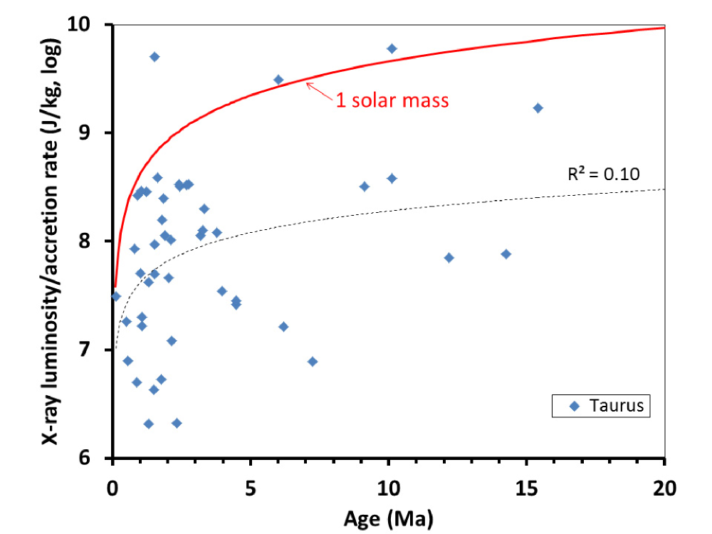
Figure 5: Plot of $L_{X}/\dot{M}$ for Taurus as a function of age (data from Güdel et al. (2007)). Although a least-square fit (dashed line) shows a systematic increase with age, scatter is evident, in part owing to the diversity of stellar masses. Overplotted is the curve (red, continuous) corresponding to one solar-mass (Telleschi et al. (2007); see beginning of section 4.2). For reference, the normalizations used in equation (4.1) amount to $L_{X}/\dot{M}=10^{7.7}\>\rm J/kg$.

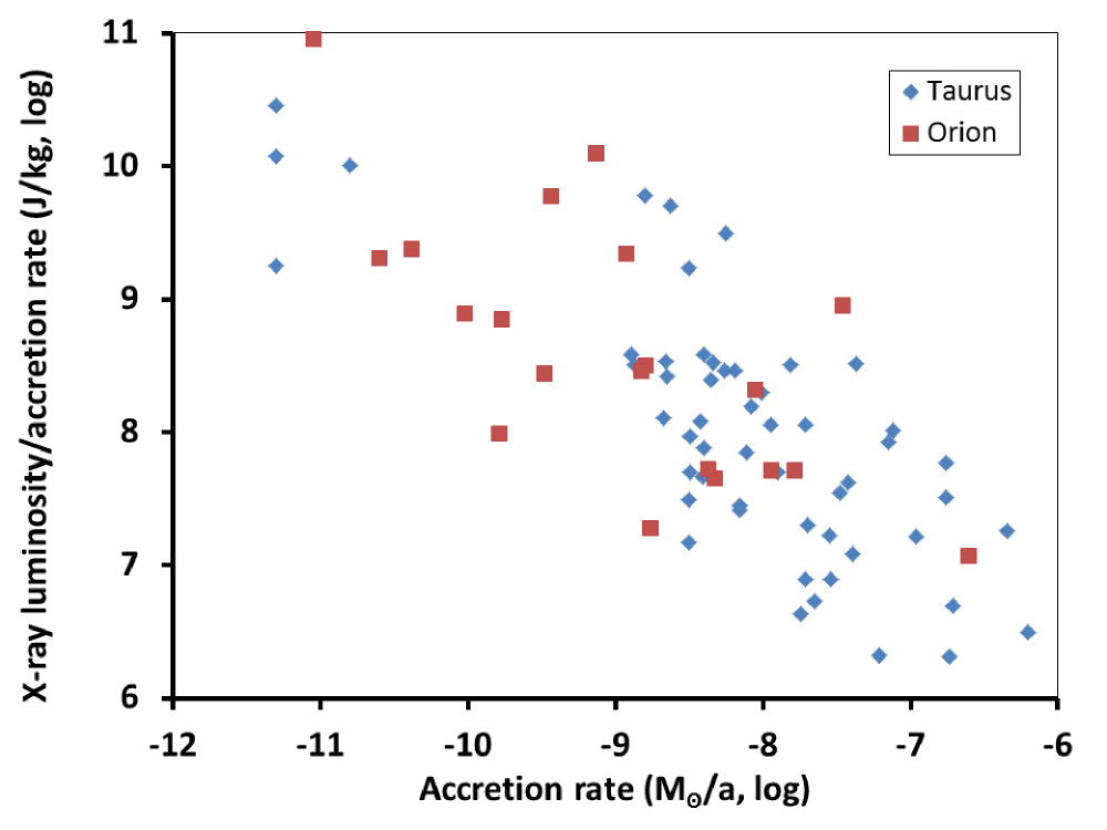
Figure 6: Plot of $L_{X}/\dot{M}$ for young stellar objects as a function of $\dot{M}$. Taurus and Orion data are taken from Güdel et al. (2007) and Bustamante et al. (2016), respectively (where $L_{X}/\dot{M}$ also shows little systematic trend with stellar mass).

In this model, ¹⁰Be/⁹Be is proportional to the $L_{X}/\dot{M}$ which is an observable. Since $L_{X}$ has only a shallow dependence on time (e.g. $\propto t^{-0.36}$ for one solar mass according to Telleschi et al. 2007), compared to the decrease of the accretion rate ($\propto t^{-1.4}$ according to Hartmann et al. 1998), $L_{X}/\dot{M}$ should increase over time (as $t^{1.04}$ if I combine these examples although derived from different data sources; see Fig. 5). It may indeed be verified in Fig. 6 that $L_{X}/\dot{M}$ anticorrelates with $\dot{M}$, if with a fair amount of scatter which remind us of the elusive determinants of $L_{X}$. Since, with decreasing $\dot{M}$, isotherms should recede toward the Sun (see equation (4)), $f_{\rm sum}$ may also be expected to increase for a given $T(R_{1})$ (e.g. a condensation front ) for a fixed magnetic field configuration. So, barring a strong decrease of $L_{10}/L_{X}$, ¹⁰Be/⁹Be should increase with time for a given formation and/or equilibration temperature. That is, mass loss from the disk would increase the relative importance of the surficial layers prone to spallation, overcoming the decline in proton luminosity.

This expectation would provide an explanation for the lower ¹⁰Be/⁹Be of FUN CAIs in CV chondrites (MacPherson et al. 2003; Wielandt et al. 2012) and PLACs in CM chondrites (Liu et al. 2010) compared to ”‘regular”’ CAIs. Indeed these CAIs are characterized by nucleosynthetic stable isotopic anomalies (e.g. in Ti, Ca; MacPherson 2014; Kööp et al. 2018) much in excess of those seen in bulk chondrules (Gerber et al. 2017) or meteorites (Trinquier et al. 2009). This suggests they formed early, perhaps during infall of an isotopically heterogeneous protosolar cloud, before turbulent mixing essentially suppressed the heterogeneities (e.g. Boss2012). Perhaps the $L_{X}/\dot{M}$ was so low that their ¹⁰Be/⁹Be was in fact dominated by the background inherited from the protosolar cloud (with perhaps some irradiation from the protostar directly on the envelope before arrival on the disk; Ceccarellietal2014) rather than later-dominating local spallation (Liu et al. 2010; Wielandt et al. 2012).

On the other end of the spectrum, a relatively late formation might explain the high ¹⁰Be/⁹Be ($7\times 10^{-3}$) of fine-grained CV chondrite CAIs analyzed by Sossi et al. (2017) or that of Isheyevo CAI 411 ($10^{-2}$; Gounelle et al. 2013). Indeed the former CAIs have group II rare earth element patterns which are commonly ascribed to condensation in a reservoir previously depleted in an ultrarefractory condensate (e.g. Boynton 1989). One may then speculate that this preliminary fractionation took some time to complete (given the tight coupling of millimeter-size solids and gas) so group II CAIs had to be of relatively late formation. However, while Isheyevo CAI 411 shows ²⁶Al/²⁷Al$<10^{-6}$—an ²⁶Al depletion common to many CH chondrite CAIs—, the fine-grained CV chondrite CAIs tend to exhibit ²⁶Al/²⁷Al ratios no lower than their melted counterparts (MacPherson et al. 2012; Kawasakietal2019), unlike what a later formation would suggest in view of the ²⁶Al half-life of 0.72 Ma (e.g. MacPherson et al. 2012). This conclusion is however predicated on an homogeneous ²⁶Al distribution which is far from a foregone assumption in early times. In fact, the nucleosynthetic anomaly-bearing CAIs discussed above show reduced ²⁶Al/²⁷Al ($\sim 10^{-5}$; MacPherson et al. 2014; Parketal2017) indicating an increase of that ratio in the CAI-forming region between their formation epoch and that of melted CAIs, and perhaps somewhat beyond. Interestingly also, some ²⁶Al should be produced by spallation along with ¹⁰Be, for their fine-grained CAIs, Sossi et al. (2017) estimated an increase of ²⁶Al/²⁷Al of $(0.3-1.2)\times 10^{-5}$, comparable to the spread resolved by MacPherson et al. (2012) and Kawasakietal2019. At any rate, this calls into question the usefulness of ²⁶Al as a chronometer during CAI formation, although it may have become more homogenized afterward. Alternatively, the coarse-grained CAIs may have acquired ¹⁰Be/⁹Be lower than their fine-grained counterparts because of equilibration with their surroundings at higher heliocentric distances, during the localized heating events which melted them.

This very dependence of ¹⁰Be/⁹Be on heliocentric distance also implies that the comparatively younger chondrules (or other meteoritic material), which likely formed several AUs away from the Sun (so probably outside the range for in situ irradiation), need not have high ¹⁰Be/⁹Be, not to mention effects of finite time of transport or radioactive decay, as timescales for the chondrule formation epoch (0-3 Ma after CAIs; Nagashimaetal2018; ConnellyBizzarro2018) or their transport are comparable to the half-life of ¹⁰Be. For a Schmidt number of order unity, one might expect a $2\pm 1$ orders of magnitude depletion with respect to the CAI-forming region (one order of magnitude closer to the Sun), but it is difficult to narrow down. Still, no chondrule ¹⁰Be/⁹Be values are known yet since silicate crystallization there hardly fractionates Be from B (Davis and McKeegan 2014).

4.3 Implications on vanadium isotopic systematics

While it is beyond the scope of the current work to calculate effects of proton irradiation on other isotopic systems, some comments on the reinterpretation of the vanadium-50 excesses (up to 4.4 ‰) reported by Sossi et al. (2017) are in order. In this framework, spallogenic ⁵⁰V would be also dominated by inheritance from the nebula, rather than in situ production, but to a lesser extent as the target nuclei/element ratio (essentially Ti/V playing the role of O/Be; Sossi et al. 2017), between two refractory elements, would not markedly differ between a solar gas and a condensate (see second paragraph of subsection 4.1). So the contention by Koopetal2018Ne that lack of evidence of in situ production of noble gases by solar energetic production in fine-grained CAIs analyzed by Vogeletal2004 prevents a spallogenic origin for their ⁵⁰V excesses and favors mass-dependent fractionation upon condensation is not necessarily valid. Since differential attenuation of the energetic particles modifies their energy distribution at finite penetration columns the production ratio (independent of the fluence, and only dependent on $p$) of two nuclides would be affected. In particular, for a given $p$, since the reactions producing ⁵⁰V are efficient at lower energies than for ¹⁰Be (Lee et al. 1998), where attenuation is strongest, ⁵⁰V production would be comparatively lower. Thus, for given (measured) ¹⁰Be/⁹Be and $\delta^{51}$V, a steeper slope than in the formalism of Sossi et al. (2017) would be indicated (for a given target composition, which however would have to be revised to solar). Since, if we ratio equation (8) with its ⁵⁰V counterpart, the only difference with the Sossi et al. (2017) formalism is the presence of $\Sigma_{p}(E)$ in the integrals in the denominator and the numerator, one may surmise that a shift of $p$ comparable to the power law exponent of $\Sigma_{p}(E)$ in the CSDA regime (about 1.82; see Appendix B) would largely cancel out its effect and restore the observed ratio. Although a steeper $p$ would diminish ¹⁰Be production for a given $L_{10}$, this would hardly affect our conclusions given the other uncertainties discussed at the end of section 4.1. This also does not take into account the neutron contribution alluded to in subsection 2.2, which may alter inferences on the energy distribution. Clearly, a dedicated study on the simultaneous effects expected for different isotopic systems in this scenario, whose proportions are independent of the uncertainties on the fluences, would be worthwhile.

4.4 X-rays and D/H fractionation

As mentioned above, X-ray emission should accompany cosmic ray flares from the Sun. These could also leave isotopic fingerprints (though unrelated to spallation) in meteorites. Indeed Gavilan et al. (2017) linked deuterium enrichment of chondritic organic matter (previously ascribed by Remusat et al. (2006, 2009) to ionizing radiation) to X-ray irradiation near the surface of the disk. The energy fluence $F$ expected for organic matter wandering in the outer disk can be calculated with the same formalism as above if I replace $\sigma_{ki}(E)(i/\mathrm{H})_{\rm CR}(k/\mathrm{Be})_{\rm tg}$ by $E$, so I end this discussion with this short aside. For an attenuation column $\Sigma_{X}(E)=0.15\>\rm kg/m^{2}(E/1\>\rm keV)^{n}$ with $n=2.485$ and an energy distribution $EI_{X}\propto\mathrm{exp}\left(-E/(k_{B}T_{X}\right))$ with $T_{X}$ the emission temperature (Igea and Glassgold 1999), the energy-weighted average of the former (the equivalent of $K_{p}$) is $\Sigma_{X}(k_{B}T_{X})\Gamma(n+1)$. For distant part of the (flared) disk, I can use $f(R_{0},R)=H_{X}/R$ (with $H_{X}$ the X-ray absorption height, likely a few times $H$ by analogy with Appendix C) so that the net fluence has the fairly well-constrained expression (modified after equation (19)):

$$F = \Gamma(n+1)\Sigma_{X}\left(k_{B}T_{X}\right)\frac{L_{X}}{\dot{M}}\left[\frac{H_{X}}{R}\right]$$ (23)

$$= 2\times 10^{7}\>\mathrm{J/m^{2}}\left(\frac{\Gamma(n+1)}{3}\right)\left(\frac{\Sigma_{X}(1\>\rm keV)}{0.15\>\rm kg/m^{2}}\right)\left(\frac{k_{B}T_{X}}{1\>\rm keV}\right)^{n}$$

$$\left(\frac{L_{X}}{3\times 10^{23}\>\rm W}\right)\left(\frac{10^{-8}\>\rm M_{\odot}/a}{\dot{M}}\right)\left(\frac{\left[H_{X}/R\right]}{0.1}\right),$$

with $\left[H_{X}/R\right]$ the difference of $H_{X}/R$ between the locus of formation of the organic matter (or the location inward of which settling ceases to be important, i.e. the $S=1$ line of Jacquet et al. (2012); see appendix C) and that of accretion in the chondrite parent body. This is 5 orders of magnitude short of the critical fluence of $5\times 10^{27}\>\rm eV/cm^{2}=8\times 10^{12}\>\rm J/m^{2}$ indicated by the experiments of Gavilan et al. (2017) for 0.5-1.3 keV photons (and much shorter than Gavilan et al. (2017)’s astrophysical estimate as well, which erroneously used X-ray attenuation at surface layers as representative of the bulk). While the steady-state approximation may overestimate the surface density in the outer regions of interest (which nevertheless should not allow efficient settling of the grains), alleviating it would hardly bridge the gap. Nevertheless, the quantitative assessment of isotopic effects of irradiation, whether X rays (in particular at higher energies) or other parts of the spectrum, is still in its infancy and this additional calculation is essentially intended for future applications in similar scenarios.

5 Conclusion

I have analytically investigated the production of short-lived radionuclide beryllium-10 in surface layers of the disk irradiated by protosolar flares. I found that ¹⁰Be production in the gas outweighs ¹⁰Be production in solids after condensation because the gas contains a greater breadth of suitable target nuclides (e.g. ¹²C, ¹H etc.) and incurs less dilution by stable refractory Be. Taking into account incipient settling and possible implantation of solar wind-borne ¹⁰Be would further widen the difference. Although many uncertainties remain on the magnetic field configuration, the scaling of cosmic rays with X-ray luminosities etc., it does appear that this model can reproduce ¹⁰Be/⁹Be ratios measured in CAIs. Therefore, the past presence of ¹⁰Be does not require (at least at present) that CAIs formed at the inner edge of the disk and allow formation at a fraction of an AU, as thermal models would suggest, and more in line with evidence for a genetic link with their host carbonaceous chondrites (abundance, fraction of the refractory budget; Jacquet et al. 2012). If this model holds true, an interesting corollary (barring strong variations of the energetic protons/X-ray ratio) is that the oldest CAIs should have the lowest ¹⁰Be/⁹Be ratios, which would explain those of nucleosynthetic anomalies-bearing CAIs ((F)UN, PLAC). This would also suggest that the fine-grained group II CAIs in CV chondrites measured by Sossi et al. (2017) were a relatively late generation of refractory inclusions, a possibility which remains to be explored. This does not mean that chondrules, which formed at comparatively much larger heliocentric distances, should have high ¹⁰Be/⁹Be, since this ratio decreases outward, following passive diffusion outside the irradiated inner disk. I finally note that the same formalism allows an estimate of fluences of X-rays (produced in the same protosolar flares) or other types of radiations, on aggregates freely floating in the disk which can be e.g. compared to experimental evidence of D/H fractionation in meteoritic organic matter by irradiation.

Appendix A Steady-state disk with infall

In this appendix, I study the effects of infall on the steady-state solution for the disk. I adopt the Cassen and Moosman (1981) expression for the infall source term per unit area $\dot{\Sigma}_{\rm in}$ for a cloud in solid-body rotation, assuming bipolar jets do not suppress it in the inner disk. The mass accretion rate is no longer constant but obeys:

$$-\frac{\partial\dot{M}}{\partial R} = 2\pi R\dot{\Sigma}_{\rm in}$$ (24)

$$= \frac{\dot{M_{\rm in}}}{2R_{C}\sqrt{1-R/R_{C}}}\theta(R_{C}-R)$$

with $R_{C}$ the instantaneous centrifugal radius, $\dot{M}_{\rm in}$ the total infall rate on the star+disk system and $\theta$ the Heaviside function. Treating all matter arriving inside $R=R_{0}$ as directly accreted by the star, this can be integrated as:

$$\dot{M}=\dot{M}_{\star}-\dot{M}_{\rm in}\left(1-\sqrt{1-\frac{R}{R_{C}}}\right),$$ (25)

with $\dot{M}_{\star}$ the mass accretion rate of the star. If the whole disk can be treated as in steady-state, we should have $\dot{M}_{\star}=\dot{M}_{\rm in}$ but I refrain from making this identification immediately as the steady-state approximation may only hold locally in the inner regions and/or in the absence of infall ($\dot{M}_{\rm in}=0$) altogether (as assumed in the main text).

Angular momentum conservation reads (Cassen and Moosman 1981):

$$\dot{M}=6\pi R^{1/2}\frac{\partial}{\partial R}\left(R^{1/2}\Sigma\nu\right)+2\pi R^{2}\Sigma\frac{\dot{M}_{\star}}{M_{\star}}+4\pi R^{2}\dot{\Sigma}_{\rm in}\left(1-\sqrt{\frac{R}{R_{C}}}\right),$$ (26)

with $M_{\star}$ the stellar mass. If the latter is much bigger than the mass of the disk, the middle term on the right-hand-side can be neglected upon integration (after division by $R^{1/2}$), which yields:

$$\left(\dot{M}_{\star}-\dot{M}_{\rm in}\right)\left(1-\sqrt{\frac{R_{0}}{R}}\right)$$

$$+\dot{M}_{\rm in}\left(\frac{R_{C}}{R}\right)^{1/2}\left[\sqrt{1-x}\left(x^{1/2}-\frac{x+2}{3}\right)\right]^{R/R_{C}}_{R_{0}/R_{C}}=3\pi\Sigma\nu.$$ (27)

For $R\ll R_{C}$ this approximates to:

$$3\pi\Sigma\nu \approx \left(\dot{M}_{\star}-\dot{M}_{\rm in}\frac{R+\sqrt{RR_{0}}+R_{0}}{2R_{C}}\right)\left(1-\sqrt{\frac{R_{0}}{R}}\right)$$ (28)

$$\approx \dot{M}\left(1-\sqrt{\frac{R_{0}}{R}}\right)\left(1-\frac{\dot{M}_{\rm in}}{\dot{M}_{\star}}\frac{\sqrt{RR_{0}}+R_{0}}{2R_{C}}\right)$$

which is thus a modest correction to equation (2).

For $R\gg R_{0}$ and $\dot{M}_{\star}=\dot{M}_{\rm in}$, I have:

$$\dot{M}_{\rm in}\Bigg{[}\sqrt{1-\frac{R}{R_{C}}}\Bigg{(}1 - \frac{\left(R/R_{C}\right)^{1/2}}{3}\Bigg{)}+\frac{2}{3}\left(\frac{R_{C}}{R}\right)^{1/2}\left(1-\sqrt{1-\frac{R}{R_{C}}}\right)\Bigg{]}$$ (29)

$$= 3\pi\Sigma\nu.$$

The factor between brackets decreases from 1 to 2/3 when $R$ increases from 0 to $R_{C}$. Beyond the centrifugal radius, $\dot{M}=0$ and, from equation (26), $R^{1/2}\Sigma\nu$ becomes constant so that:

$$3\pi\Sigma\nu=\frac{2}{3}\dot{M}_{\rm in}\left(\frac{R_{C}}{R}\right)^{1/2}$$ (30)

For bounded $\alpha T$, $2\pi R\Sigma$ is not integrable, but this steady-state solution, which merely sets an upper bound to the disk viscous expansion, can only hold for distances of $t_{\rm vis}(R)$ shorter than the timescale of evolution of the system.

Appendix B Calculation of $K_{p}$

I take the attenuation column for protons as the minimum between the continuous slowing-down approximation (CSDA) and diffusion regimes of Padovani et al. (2018), after integrating their equations E.3 and 21, respectively:

$$\Sigma_{p,H}(E) = m\mathrm{min}\left[\frac{E^{1+s}}{A\left(p-1\right)},\frac{1}{2(p-1)}\sqrt{\frac{E\left(\alpha_{p}-1\right)}{3\sigma_{MT}L_{p}(E)}}\frac{\Gamma\left(\frac{p-1}{\alpha_{p}-1}+1\right)}{\Gamma\left(\frac{p-1}{\alpha_{p}-1}+\frac{1}{2}\right)}\right]$$ (32)

$$= \frac{1}{p-1}\mathrm{min}\Bigg{[}1.2\>\rm kg/m^{2}\left(\frac{E}{10\>\rm MeV}\right)^{1.82},$$

$$6\times 10^{2}\>\rm kg/m^{2}\left(\frac{1\>\rm GeV}{E}\right)^{0.14}\frac{\Gamma\left(\frac{p-1}{\alpha_{p}-1}+1\right)}{\Gamma\left(\frac{p-1}{\alpha_{p}-1}+\frac{1}{2}\right)}\Bigg{]}$$

where $A=1.77\times 10^{-6}\>\rm eV^{1+s}m^{2}$, $s=0.82$, $\alpha_{p}=1.28$ (noted $\alpha$ in Padovani et al. (2018)), $\sigma_{MT}=10^{-30}\>\rm m^{2}$, $L_{p}(E)=10^{-21}\>\rm m^{2}eV(E/\rm GeV)^{\alpha_{p}}$ are defined in Padovani et al. (2018) and $\Gamma$ is Euler’s gamma function. For the other species, I adopt $\Sigma_{p,i}=\Sigma_{p,H}A_{i}/Z_{i}^{2}$, with $Z_{i}$, $A_{i}$ its atomic and mass numbers of species $i$ (e.g. Gounelle et al. 2001). The transition between the CSDA and the diffusion regime thus occurs at:

$$E_{\rm crit}=0.33\>\rm GeV\left(\frac{\Gamma\left(\frac{p-1}{\alpha_{p}-1}+1\right)}{\Gamma\left(\frac{p-1}{\alpha_{p}-1}+\frac{1}{2}\right)}\right)^{0.51}$$ (33)

As to the cross sections, similar to Desch et al. (2004), I adopt the Yanasak et al. (2001) formulation

$$\sigma_{ki}(E)=\sigma_{0}\mathrm{min}\left(\left(\frac{E}{E_{0}}\right)^{x},1\right)\theta(E-E_{\rm th})$$ (34)

with $\sigma_{0}$, $E_{\rm th}$, $E_{0}$, $x$ constants (for a given $(k,i)$) and $\theta$ is again the Heaviside function. I fitted those for $i=^{4}$He using the Lange et al. (1995) data (unknown to Yanasak et al. (2001)), with power-law fitting below 30 MeV/nucleon and the flat regime being assigned the maximum cross section measured (rather than a fit beyond the aforementioned threshold, as this regime is only incipient in the energy range studied). The resulting parameters are presented in table 1.

Table 1: Cross section parameters

Reaction	$E_{\rm th}$ (MeV)	$\sigma_{0}$ (mb)	$E_{0}$ (MeV)	$x$
12C(p,x)10Be	27.4	3.79	1037	0.53
14N(p,x)10Be	32.1	1.75	671	0.715
16O(p,x)10Be	34.6	2.52	798	0.962
12C($\alpha$,x)10Be	19.675	9.38	34	1.4
14N($\alpha$,x)10Be	11.05	5.26	30	3.4
16O($\alpha$,x)10Be	13.45	4.35	29	4.3

Then, I have, for $E_{\rm th}\leq E_{0}\leq E_{\rm crit}$:

$$\int_{0}^{+\infty}\sigma_{ki}(E)\Sigma_{p,i}E^{-p}\mathrm{d}E=\sigma_{0}\frac{\Sigma_{p,i}^{\rm CSDA}(E_{0})}{E_{0}^{p-1}}\Bigg{(}\frac{1-(E_{\rm th}/E_{0})^{2+s+x-p}}{2+s+x-p}$$

$$+\frac{(E_{\rm crit}/E_{0})^{2+s-p}-1}{2+s-p}+\frac{(E_{\rm crit}/E_{0})^{2+s-p}}{p+(\alpha_{p}-3)/2}\Bigg{)},$$ (35)

and for $E_{\rm th}\leq E_{\rm crit}\leq E_{0}$:

$$\int_{0}^{+\infty}\sigma_{ki}(E)\Sigma_{p,i}E^{-p}\mathrm{d}E$$

$$=\sigma_{0}\frac{\Sigma_{p,i}^{\rm CSDA}(E_{0})}{E_{0}^{p-1}}\Bigg{(}\frac{(E_{\rm crit}/E_{0})^{2+s+x-p}-(E_{\rm th}/E_{0})^{2+s+x-p}}{2+s+x-p}$$

$$+\frac{(E_{\rm crit}/E_{0})^{s+(\alpha_{p}+1)/2}-(E_{\rm crit}/E_{0})^{2+s+x-p}}{x-p-(\alpha_{p}-3)/2}+\frac{(E_{\rm crit}/E_{0})^{s+(\alpha_{p}+1)/2}}{p+(\alpha_{p}-3)/2}\Bigg{)},$$ (36)

whose contributions can be summed to yield $K_{p}$ (equation (10)).

Appendix C Height of spallation layer and effect of settling on ¹⁰Be production in solids

The spallation layer column $\Sigma_{\rm spall}$ may be defined as:

$$\Sigma_{\rm spall}\equiv\frac{1}{\left(\overset{\bullet}{{}^{10}\rm Be}/^{9}\rm Be\right)_{\rm tg,+}(0)}\int_{0}^{+\infty}\left(\frac{\overset{\bullet}{{}^{10}\rm Be}}{{}^{9}\rm Be}\right)_{\rm tg,+}\mathrm{d}\Sigma^{\prime}=\langle\Sigma_{p}(E)\rangle_{\sigma E^{-p}}\frac{\mathrm{sin}\phi}{2}$$ (37)

Assuming a vertically isothermal disk (and thus a gaussian gas density $\rho(z)=\Sigma\mathrm{exp}(-(z/H)^{2}/2)/(\sqrt{2\pi}H)$), the height $H_{\rm spall}$ of this layer obeys:

$$\Sigma_{\rm spall}=\frac{\Sigma}{2}\mathrm{erfc}\left(\frac{H_{\rm spall}}{H\sqrt{2}}\right).$$ (38)

For $\Sigma\sim 10^{5\pm 1}\>\rm kg/m^{2}$ and $\Sigma_{\rm spall}=10^{1\pm 1}\>\mathrm{kg/m^{2}}$, I have $\chi\equiv H_{\rm spall}/H\approx 3\pm 1$, so that:

$$\frac{H_{\rm spall}}{R}=0.16\left(\frac{\chi}{3}\right)\left(\frac{R}{0.5\>\rm AU}\right)^{1/2}\left(\frac{T}{1500\>\rm K}\right)^{1/2}.$$ (39)

Since, for $x\gtrsim 2$, I have

$$\mathrm{erfc}(x)\approx\frac{\mathrm{exp}(-x^{2})}{\sqrt{\pi}x},$$ (40)

the density at $z=H_{\rm spall}$ may be approximated as:

$$\rho(H_{\rm spall})=\frac{\chi\Sigma_{\rm spall}}{H}=8\times 10^{-9}\>\mathrm{kg/m^{3}}\left(\frac{\chi}{3}\right)\left(\frac{\Sigma_{\rm spall}}{10\>\rm kg/m^{2}}\right)\left(\frac{1500\>\rm K}{T}\right)^{1/2}$$

$$\left(\frac{0.5\>\rm AU}{R}\right)^{3/2}.$$ (41)

The nominal value (corresponding to a number density of $2\times 10^{12}\>\rm cm^{-3}$) is half-way in the range studied by Umebayashi and Nakano (1981) so the neutron contribution (ignored in this paper) can be seen in their Fig. 2 and 5 to be limited. Then, the settling parameter (Jacquet et al. 2012) for a solid of density $\rho_{s}$ and radius $a$ there is:

$$S_{z}(H_{\rm spall}) = \sqrt{\frac{\pi}{8}}\frac{\rho_{s}a}{\rho(H_{\rm spall})c_{s}\delta_{z}}$$ (42)

$$\approx \sqrt{\frac{\pi}{8}}\frac{\rho_{s}a}{\Sigma_{\rm spall}\delta_{z}\chi}$$

$$= 0.2\left(\frac{\rho_{s}a}{1\>\rm kg/m^{2}}\right)\left(\frac{10\>\rm kg/m^{2}}{\Sigma_{\rm spall}}\right)\left(\frac{10^{-1}}{\delta_{z}}\right)\left(\frac{3}{\chi}\right)$$

with $\delta_{z}$ the vertical diffusion coefficient normalized to $c_{s}^{2}/\Omega_{K}$ (which should be of order $\alpha$).

Simulations of ideal MHD turbulence indicate $\delta_{z}\sim\alpha\propto\rho^{-1}$ over a large extent of the disk thickness, although it should stall in the corona (e.g. Jacquet 2013, and references therein). Since $S_{z}$ may be expected to be $\lesssim 1$ there from the above evaluation, it may not be a dramatic underestimate to treat it as constant throughout the vertical thickness of the disk. Under that assumption, a population of identical solids has a density (Jacquet 2013)

$$\rho_{c}(z)=\frac{\Sigma_{c}\sqrt{1+S_{z}}}{\sqrt{2\pi}H}\mathrm{exp}\left(-\frac{S_{z}+1}{2}\left(\frac{z}{H}\right)^{2}\right)$$ (43)

with $\Sigma_{c}$ the surface density of the population. The ¹⁰Be production rate averaged over this distribution is then

$$\left\langle\left(\frac{\overset{\bullet}{{}^{10}\rm Be}}{{}^{9}\rm Be}\right)_{\rm tg}\right\rangle_{\rho_{c}}\equiv\frac{2}{\Sigma_{c}}\int_{0}^{+\infty}\mathrm{d}\Sigma_{c}^{\prime}\left(\frac{\overset{\bullet}{{}^{10}\rm Be}}{{}^{9}\rm Be}\right)_{\rm tg,+}\left(\Sigma^{\prime}(\Sigma_{p}^{\prime})\right)$$ (44)

with $\Sigma_{c}^{\prime}$ and $\Sigma^{\prime}$ the columns of the solids and gas, respectively, integrated vertically from the surface. If I let

$$\left(\frac{\overset{\bullet}{{}^{10}\rm Be}}{{}^{9}\rm Be}\right)_{\rm tg,+}\equiv\left(\frac{\overset{\bullet}{{}^{10}\rm Be}}{{}^{9}\rm Be}\right)_{\rm tg,+}(0)g\left(\frac{\Sigma^{\prime}}{\Sigma_{\rm spall}}\right),$$ (45)

and since

$$\Sigma^{\prime}=\frac{\Sigma}{2}\mathrm{erfc}\left(\frac{\mathrm{erfc}^{-1}\left(2\Sigma_{c}^{\prime}/\Sigma_{c}\right)}{\sqrt{1+S_{z}}}\right),$$ (46)

this becomes:

$$\left\langle\left(\frac{\overset{\bullet}{{}^{10}\rm Be}}{{}^{9}\rm Be}\right)_{\rm tg}\right\rangle_{\rho_{c}} = \frac{\Sigma}{2\Sigma_{\rm spall}}\int_{0}^{+\infty}g\left(\frac{\Sigma}{2\Sigma_{\rm spall}}\mathrm{erfc}\left(\frac{\mathrm{erfc}^{-1}(x)}{\sqrt{1+S_{z}}}\right)\right)\mathrm{d}x\left\langle\left(\frac{\overset{\bullet}{{}^{10}\rm Be}}{{}^{9}\rm Be}\right)_{\rm tg}\right\rangle_{\rho}$$ (47)

$$\approx \frac{\Sigma}{2\Sigma_{\rm spall}}\int_{0}^{+\infty}g\left(\frac{\Sigma}{2\Sigma_{\rm spall}}\frac{x^{1/(S_{z}+1)}\sqrt{S_{z}+1}}{\left(\sqrt{\pi}\mathrm{erfc}^{-1}(x)\right)^{S_{z}/(S_{z}+1)}}\right)\mathrm{d}x$$

$$\left\langle\left(\frac{\overset{\bullet}{{}^{10}\rm Be}}{{}^{9}\rm Be}\right)_{\rm tg}\right\rangle_{\rho}$$

where I have used approximation (40),with the corollary $\mathrm{erfc}^{-1}(z)\approx\sqrt{-\mathrm{ln}(\sqrt{\pi}z\mathrm{erfc}^{-1}(z))}$ for $z\ll 1$. Roughly speaking, the integrand only contributes ($\sim 1$) for a $g$ argument $\lesssim 1$, that is $x\lesssim(\sqrt{\pi}\mathrm{erfc}^{-1}(x))^{S_{z}}(2\Sigma_{\rm spall}/\Sigma\sqrt{S_{z}+1})^{S_{z}+1}$ so that:

$$\left\langle\left(\frac{\overset{\bullet}{{}^{10}\rm Be}}{{}^{9}\rm Be}\right)_{\rm tg}\right\rangle_{\rho_{c}}\sim\frac{1}{\sqrt{S_{z}+1}}\left(\sqrt{\pi\mathrm{ln}(\Sigma/\Sigma_{\rm spall})}\frac{2\Sigma_{\rm spall}}{\Sigma}\right)^{S_{z}}\left\langle\left(\frac{\overset{\bullet}{{}^{10}\rm Be}}{{}^{9}\rm Be}\right)_{\rm tg}\right\rangle_{\rho}.$$ (48)

So ¹⁰Be production should quickly drop as $S_{z}$ approaches unity and become negligible for $S_{z}\gtrsim 1$.

References

- Bai (2016) Bai, X.-N. (2016). Towards a Global Evolutionary Model of Protoplanetary Disks. The Astrophysical Journal, 821, 80.
- Balbus and Hawley (1998) Balbus, S. A. and Hawley, J. F. (1998). Instability, turbulence, and enhanced transport in accretion disks. Reviews of Modern Physics, 70, 1–53.
- Boynton (1989) Boynton, W. V. (1989). Cosmochemistry of the rare earth elements: condensation and evaporation processes. In R. B. Lipin and G. A. McKay, editors, Geochemistry and mineralogy of the rare earth elements, volume 21, chapter 1, pages 1–24. Mineralogical Society of America, Chantilly.
- Bricker and Caffee (2010) Bricker, G. E. and Caffee, M. W. (2010). Solar Wind Implantation Model for 10Be in Calcium-Aluminum Inclusions. The Astrophysical Journal, 725, 443–449.
- Burkhardt et al. (2018) Burkhardt, C., Dauphas, N., Hans, U., Bourdon, B., and Kleine, T. (2018). Isotope Anomalies in Chondrite Components as Tracers of Nebular Material Processing and Disk Dynamics. LPI Contributions, 2067, 6289.
- Bustamante et al. (2016) Bustamante, I., Merín, B., Bouy, H., Manara, C. F., Ribas, Á., and Riviere-Marichalar, P. (2016). X-ray deficiency on strongly accreting T Tauri stars. Comparing Orion with Taurus. Astronomy & Astrophysics, 587, A81.
- Cassen and Moosman (1981) Cassen, P. and Moosman, A. (1981). On the formation of protostellar disks. Icarus, 48, 353–376.
- Ciesla (2010) Ciesla, F. J. (2010). Residence Times of Particles in Diffusive Protoplanetary Disk Environments. I. Vertical Motions. The Astrophysical Journal, 723, 514–529.
- Clarke and Pringle (1988) Clarke, C. J. and Pringle, J. E. (1988). The diffusion of contaminant through an accretion disc. Monthly Notices of the Royal Astronomical Society, 235, 365–373.
- Davis and McKeegan (2014) Davis, A. M. and McKeegan, K. D. (2014). Short-Lived Radionuclides and Early Solar System Chronology, pages 361–395. Elsevier.
- Davis and Richter (2014) Davis, A. M. and Richter, F. M. (2014). Condensation and Evaporation of Solar System Materials, pages 335–360. Elsevier.
- Desai and Giacalone (2016) Desai, M. and Giacalone, J. (2016). Large gradual solar energetic particle events. Living Reviews in Solar Physics, 13, 3.
- Desch et al. (2004) Desch, S. J., Connolly, Jr., H. C., and Srinivasan, G. (2004). An Interstellar Origin for the Beryllium 10 in Calcium-rich, Aluminum-rich Inclusions. The Astrophysical Journal, 602, 528–542.
- Desch et al. (2010) Desch, S. J., Morris, M. A., Connolly, Jr., H. C., and Boss, A. P. (2010). A Critical Examination of the X-wind Model for Chondrule and Calcium-rich, Aluminum-rich Inclusion Formation and Radionuclide Production. The Astrophysical Journal, 725, 692–711.
- Ebert and Bischoff (2016) Ebert, S. and Bischoff, A. (2016). Genetic relationship between Na-rich chondrules and Ca,Al-rich inclusions? - Formation of Na-rich chondrules by melting of refractory and volatile precursors in the solar nebula. Geochimica et Cosmochimica Acta, 177, 182–204.
- Emslie et al. (2012) Emslie, A. G., Dennis, B. R., Shih, A. Y., Chamberlin, P. C., Mewaldt, R. A., Moore, C. S., Share, G. H., Vourlidas, A., and Welsch, B. T. (2012). Global Energetics of Thirty-eight Large Solar Eruptive Events. The Astrophysical Journal, 759, 71.
- Feigelson et al. (2002) Feigelson, E. D., Garmire, G. P., and Pravdo, S. H. (2002). Magnetic Flaring in the Pre-Main-Sequence Sun and Implications for the Early Solar System. The Astrophysical Journal, 572, 335–349.
- Gavilan et al. (2017) Gavilan, L., Remusat, L., Roskosz, M., Popescu, H., Jaouen, N., Sandt, C., Jäger, C., Henning, T., Simionovici, A., Lemaire, J. L., Mangin, D., and Carrasco, N. (2017). X-Ray-induced Deuterium Enrichment of N-rich Organics in Protoplanetary Disks: An Experimental Investigation Using Synchrotron Light. The Astrophysical Journal, 840, 35.
- Gerber et al. (2017) Gerber, S., Burkhardt, C., Budde, G., Metzler, K., and Kleine, T. (2017). Mixing and Transport of Dust in the Early Solar Nebula as Inferred from Titanium Isotope Variations among Chondrules. The Astrophysical Journal Letters, 841, L17.
- Gounelle et al. (2001) Gounelle, M., Shu, F. H., Shang, H., Glassgold, A. E., Rehm, K. E., and Lee, T. (2001). Extinct Radioactivities and Protosolar Cosmic Rays: Self-Shielding and Light Elements. The Astrophysical Journal, 548, 1051–1070.
- Gounelle et al. (2006) Gounelle, M., Shu, F. H., Shang, H., Glassgold, A. E., Rehm, K. E., and Lee, T. (2006). The Irradiation Origin of Beryllium Radioisotopes and Other Short-lived Radionuclides. The Astrophysical Journal, 640, 1163–1170.
- Gounelle et al. (2013) Gounelle, M., Chaussidon, M., and Rollion-Bard, C. (2013). Variable and Extreme Irradiation Conditions in the Early Solar System Inferred from the Initial Abundance of 10Be in Isheyevo CAIs. The Astrophysical Journal Letters, 763, L33.
- Grossman (2010) Grossman, L. (2010). Vapor-condensed phase processes in the early solar system. Meteoritics and Planetary Science, 45, 7–20.
- Güdel et al. (2007) Güdel, M., Skinner, S. L., Mel’Nikov, S. Y., Audard, M., Telleschi, A., and Briggs, K. R. (2007). X-rays from T Tauri: a test case for accreting T Tauri stars. Astronomy & Astrophysics, 468, 529–540.
- Hartmann et al. (1998) Hartmann, L., Calvet, N., Gullbring, E., and D’Alessio, P. (1998). Accretion and the Evolution of T Tauri Disks. The Astrophysical Journal, 495, 385–400.
- Hezel et al. (2008) Hezel, D. C., Russell, S. S., Ross, A. J., and Kearsley, A. T. (2008). Modal abundances of CAIs: Implications for bulk chondrite element abundances and fractionations. Meteoritics and Planetary Science, 43, 1879–1894.
- Igea and Glassgold (1999) Igea, J. and Glassgold, A. E. (1999). X-Ray Ionization of the Disks of Young Stellar Objects. The Astrophysical Journal, 518, 848–858.
- Jacquet (2013) Jacquet, E. (2013). On vertical variations of gas flow in protoplanetary disks and their impact on the transport of solids. Astronomy & Astrophysics, 551, A75.
- Jacquet (2014) Jacquet, E. (2014). Transport of solids in protoplanetary disks: Comparing meteorites and astrophysical models. Comptes Rendus Geoscience, 346, 3–12.
- Jacquet and Marrocchi (2017) Jacquet, E. and Marrocchi, Y. (2017). Chondrule heritage and thermal histories from trace element and oxygen isotope analyses of chondrules and amoeboid olivine aggregates. Meteoritics and Planetary Science, 52, 2672–2694.
- Jacquet and Robert (2013) Jacquet, E. and Robert, F. (2013). Water transport in protoplanetary disks and the hydrogen isotopic composition of chondrites. Icarus, 223, 722–732.
- Jacquet et al. (2012) Jacquet, E., Gounelle, M., and Fromang, S. (2012). On the aerodynamic redistribution of chondrite components in protoplanetary disks. Icarus, 220, 162–173.
- Johansen et al. (2006) Johansen, A., Klahr, H., and Mee, A. J. (2006). Turbulent diffusion in protoplanetary discs: the effect of an imposed magnetic field. Monthly Notices of the Royal Astronomical Society, 370, L71–L75.
- Jones and Schilk (2009) Jones, R. H. and Schilk, A. J. (2009). Chemistry, petrology and bulk oxygen isotope compositions of chondrules from the Mokoia CV3 carbonaceous chondrite. Geochimica et Cosmochimica Acta, 73, 5854–5883.
- Kööp et al. (2018) Kööp, L., Nakashima, D., Heck, P. R., Kita, N. T., Tenner, T. J., Krot, A. N., Nagashima, K., Park, C., and Davis, A. M. (2018). A multielement isotopic study of refractory FUN and F CAIs: Mass-dependent and mass-independent isotope effects. Geochimica et Cosmochimica Acta, 221, 296–317.
- Krot et al. (2004) Krot, A., Petaev, M., Russell, S. S., Itoh, S., Fagan, T. J., Yurimoto, H., Chizmadia, L., Weisberg, M. K., Kornatsu, M., Ulyanov, A. A., and Keil, K. (2004). Amoeboid olivine aggregates and related objects in carbonaceous chondrites: records of nebular and asteroid processes. Chemie der Erde / Geochemistry, 64, 185–239.
- Lange et al. (1995) Lange, H.-J., Hahn, T., R., M., Schiekel, T., Rösel, R., Herpers, U., Hofmann, H.-J., Dittrich-Hannen, B., Suter, M., Wölfli, W., and Kubik, P. W. (1995). Production of residual nuclei by -induced reactions on c, n, o, mg, al and si up to 170 mev. Applied Radiation and Isotopes, 46(2), 93–112.
- Lee et al. (1998) Lee, T., Shu, F. H., Shang, H., Glassgold, A. E., and Rehm, K. E. (1998). Protostellar Cosmic Rays and Extinct Radioactivities in Meteorites. The Astrophysical Journal, 506, 898–912.
- Liu et al. (2009) Liu, M.-C., McKeegan, K. D., Goswami, J. N., Marhas, K. K., Sahijpal, S., Ireland, T. R., and Davis, A. M. (2009). Isotopic records in CM hibonites: Implications for timescales of mixing of isotope reservoirs in the solar nebula. Geochimica et Cosmochimica Acta, 73, 5051–5079.
- Liu et al. (2010) Liu, M.-C., Nittler, L. R., Alexander, C. M. O., and Lee, T. (2010). Lithium-Beryllium-Boron Isotopic Compositions in Meteoritic Hibonite: Implications for Origin of 10Be and Early Solar System Irradiation. The Astronomical Journal Letters, 719, L99–L103.
- Lodders (2003) Lodders, K. (2003). Solar System Abundances and Condensation Temperatures of the Elements. The Astrophysical Journal, 591, 1220–1247.
- Lugaro et al. (2018) Lugaro, M., Ott, U., and Kereszturi, Á. (2018). Radioactive nuclei from cosmochronology to habitability. Progress in Particle and Nuclear Physics, 102, 1–47.
- MacPherson (2014) MacPherson, G. J. (2014). Calcium-Aluminum-Rich Inclusions in Chondritic Meteorites, pages 139–179.
- MacPherson et al. (2003) MacPherson, G. J., Huss, G. R., and Davis, A. M. (2003). Extinct 10Be in Type A calcium-aluminum-rich inclusions from CV chondrites. Geochimica et Cosmochimica Acta, 67, 3165–3179.
- MacPherson et al. (2012) MacPherson, G. J., Kita, N. T., Ushikubo, T., Bullock, E. S., and Davis, A. M. (2012). Well-resolved variations in the formation ages for Ca-Al-rich inclusions in the early Solar System. Earth and Planetary Science Letters, 331, 43–54.
- MacPherson et al. (2014) MacPherson, G. J., Davis, A. M., and Zinner, E. K. (2014). Distribution of 26Al in the Early Solar System: A 2014 Reappraisal. In Lunar and Planetary Science Conference, volume 45 of Lunar and Planetary Science Conference, page 2134.
- Marrocchi et al. (2018) Marrocchi, Y., Villeneuve, J., Batanova, V., Piani, L., and Jacquet, E. (2018). Oxygen isotopic diversity of chondrule precursors and the nebular origin of chondrules. Earth and Planetary Science Letters, 496, 132–141.
- McKeegan et al. (2000) McKeegan, K. D., Chaussidon, M., and Robert, F. (2000). Incorporation of Short-Lived 10Be in a Calcium-Aluminum-Rich Inclusion from the Allende Meteorite. Science, 289, 1334–1337.
- Metzler and Pack (2016) Metzler, K. and Pack, A. (2016). Chemistry and oxygen isotopic composition of cluster chondrite clasts and their components in LL3 chondrites. Meteoritics and Planetary Science, 51, 276–302.
- Mewaldt (2006) Mewaldt, R. A. (2006). Solar Energetic Particle Composition, Energy Spectra, and Space Weather. Space Science Review, 124, 303–316.
- Mewaldt et al. (2007) Mewaldt, R. A., Cohen, C. M. S., Mason, G. M., Cummings, A. C., Desai, M. I., Leske, R. A., Raines, J., Stone, E. C., Wiedenbeck, M. E., von Rosenvinge, T. T., and Zurbuchen, T. H. (2007). On the Differences in Composition between Solar Energetic Particles and Solar Wind. Space Science Review, 130, 207–219.
- Misawa and Nakamura (1988) Misawa, K. and Nakamura, N. (1988). Demonstration of REE fractionation among individual chondrules from the Allende (CV3) chondrite. Geochimica et Cosmochimica Acta, 52, 1699–1710.
- Nishiizumi and Caffee (2001) Nishiizumi, K. and Caffee, M. W. (2001). Beryllium-10 from the Sun. Science, 294, 352–354.
- Padovani et al. (2018) Padovani, M., Ivlev, A. V., Galli, D., and Caselli, P. (2018). Cosmic-ray ionisation in circumstellar discs. Astronomy & Astrophysics, 614, A111.
- Papaioannou et al. (2016) Papaioannou, A., Sandberg, I., Anastasiadis, A., Kouloumvakos, A., Georgoulis, M. K., Tziotziou, K., Tsiropoula, G., Jiggens, P., and Hilgers, A. (2016). Solar flares, coronal mass ejections and solar energetic particle event characteristics. Journal of Space Weather and Space Climate, 6(27), A42.
- Paque et al. (2014) Paque, J. M., Burnett, D. S., Beckett, J. R., and Guan, Y. (2014). CAI Refractory Lithophile Trace Element Distributions: Implications for Radiogenic Isotopes. In Lunar and Planetary Science Conference, volume 45 of Lunar and Planetary Inst. Technical Report, page 2176.
- Preibisch et al. (2005) Preibisch, T., Kim, Y.-C., Favata, F., Feigelson, E. D., Flaccomio, E., Getman, K., Micela, G., Sciortino, S., Stassun, K., Stelzer, B., and Zinnecker, H. (2005). The Origin of T Tauri X-Ray Emission: New Insights from the Chandra Orion Ultradeep Project. The Astrophysical Journal Supplement Series, 160, 401–422.
- Reedy (1996) Reedy, R. C. (1996). Constraints on Solar Particle Events from Comparisons of Recent Events and Million-Year Averages. In K. S. Balasubramaniam, S. L. Keil, and R. N. Smartt, editors, Solar Drivers of the Interplanetary and Terrestrial Disturbances, volume 95 of Astronomical Society of the Pacific Conference Series, page 429.
- Remusat et al. (2006) Remusat, L., Palhol, F., Robert, F., Derenne, S., and France-Lanord, C. (2006). Enrichment of deuterium in insoluble organic matter from primitive meteorites: A solar system origin? Earth and Planetary Science Letters, 243, 15–25.
- Remusat et al. (2009) Remusat, L., Robert, F., Meibom, A., Mostefaoui, S., Delpoux, O., Binet, L., Gourier, D., and Derenne, S. (2009). Proto-Planetary Disk Chemistry Recorded by D-Rich Organic Radicals in Carbonaceous Chondrites. The Astrophysical Journal, 698, 2087–2092.
- Shu et al. (2001) Shu, F. H., Shang, H., Gounelle, M., Glassgold, A. E., and Lee, T. (2001). The Origin of Chondrules and Refractory Inclusions in Chondritic Meteorites. The Astrophysical Journal, 548, 1029–1050.
- Sossi et al. (2017) Sossi, P. A., Moynier, F., Chaussidon, M., Villeneuve, J., Kato, C., and Gounelle, M. (2017). Early Solar System irradiation quantified by linked vanadium and beryllium isotope variations in meteorites. Nature Astronomy, 1, 0055.
- Telleschi et al. (2007) Telleschi, A., Güdel, M., Briggs, K. R., Audard, M., and Palla, F. (2007). X-ray emission from T Tauri stars and the role of accretion: inferences from the XMM-Newton extended survey of the Taurus molecular cloud. Astronomy & Astrophysics, 468, 425–442.
- Trinquier et al. (2009) Trinquier, A., Elliott, T., Ulfbeck, D., Coath, C., Krot, A. N., and Bizzarro, M. (2009). Origin of Nucleosynthetic Isotope Heterogeneity in the Solar Protoplanetary Disk. Science, 324, 374–376.
- Umebayashi and Nakano (1981) Umebayashi, T. and Nakano, T. (1981). Fluxes of Energetic Particles and the Ionization Rate in Very Dense Interstellar Clouds. PASJ, 33, 617.
- Wielandt et al. (2012) Wielandt, D., Nagashima, K., Krot, A. N., Huss, G. R., Ivanova, M. A., and Bizzarro, M. (2012). Evidence for Multiple Sources of 10Be in the Early Solar System. The Astrophysical Journal Letters, 748, L25.
- Wolk et al. (2005) Wolk, S. J., Harnden, Jr., F. R., Flaccomio, E., Micela, G., Favata, F., Shang, H., and Feigelson, E. D. (2005). Stellar Activity on the Young Suns of Orion: COUP Observations of K5-7 Pre-Main-Sequence Stars. The Astrophysical Journal Supplement Series, 160, 423–449.
- Wood (2004) Wood, J. A. (2004). Formation of chondritic refractory inclusions: The astrophysical setting. Geochimica et Cosmochimica Acta, 68, 4007–4021.
- Wooden et al. (2007) Wooden, D., Desch, S., Harker, D., Gail, H., and Keller, L. (2007). Comet Grains and Implications for Heating and Radial Mixing in the Protoplanetary Disk. Protostars and Planets V, pages 815–833.
- Yanasak et al. (2001) Yanasak, N. E., Wiedenbeck, M. E., Mewaldt, R. A., Davis, A. J., Cummings, A. C., George, J. S., Leske, R. A., Stone, E. C., Christian, E. R., von Rosenvinge, T. T., Binns, W. R., Hink, P. L., and Israel, M. H. (2001). Measurement of the Secondary Radionuclides 10Be, 26Al, 36Cl, 54Mn, and 14C and Implications for the Galactic Cosmic-Ray Age. The Astrophysical Journal, 563, 768–792.