Minimizers of convex functionals with small degeneracy set

Abstract.

We study the question whether Lipschitz minimizers of $\int F(\nabla u)\,dx$ in $\mathbb{R}^{n}$ are $C^{1}$ when $F$ is strictly convex. Building on work of De Silva-Savin, we confirm the $C^{1}$ regularity when $D^{2}F$ is positive and bounded away from finitely many points that lie in a $2$-plane. We then construct a counterexample in $\mathbb{R}^{4}$, where $F$ is strictly convex but $D^{2}F$ degenerates on the intersection of a Simons cone with $S^{3}$. Finally we highlight a connection between the case $n=3$ and a result of Alexandrov in classical differential geometry, and we make a conjecture about this case.

1. Introduction

In this paper we study the regularity of Lipschitz minimizers of

(1) $$E(u)=\int_{B_{1}}F(\nabla u)\,dx$$

in $\mathbb{R}^{n}$, where $F:\mathbb{R}^{n}\rightarrow\mathbb{R}$ is convex. By Lipschitz minimizer we mean a function $u\in W^{1,\,\infty}(B_{1})$ that satisfies $E(u+\varphi)\geq E(u)$ for all $\varphi\in C^{1}_{0}(B_{1})$. It is straightforward to show that Lipschitz minimizers solve the Euler-Lagrange equation

(2) $$\text{div}(\nabla F(\nabla u))=0$$

in the weak sense. Conversely, any Lipschitz weak solution of (2) is a minimizer of $E$ by the convexity of $F$.

In the extreme case that the graph of $F$ contains a line segment, minimizers are no better than Lipschitz by simple examples. In the other extreme that $F$ is smooth and uniformly convex, De Giorgi and Nash proved that Lipschitz minimizers are smooth and solve the Euler-Lagrange equation $F_{ij}(\nabla u)u_{ij}=0$ classically ([DG], [Na]). It remains largely open what happens in the intermediate case where $F$ is strictly convex, but the eigenvalues of $D^{2}F$ go to $0$ or $\infty$ on some set $D_{F}$. Such functionals arise naturally in the study of anisotropic surface tensions [DMMN], traffic flow [CF], and statistical mechanics ([CKP], [KOS]).

In [DS] the authors raise the natural question:

(3) Are Lipschitz minimizers in $$C^{1} F$$ when is strictly convex?

They give evidence that the answer may be “yes,” at least in two dimensions. In particular, they show that if $n=2$ and $D_{F}$ consists of finitely many points, then Lipschitz minimizers of $E$ are $C^{1}$. In this paper we study this question in higher dimensions. We first confirm the $C^{1}$ regularity of Lipschitz minimizers when $D_{F}$ is a finite set in some $2$-plane. In particular, this covers the case that $D_{F}$ consists of three points. We then show the answer to Question (3) is “no” in general, by constructing a singular Lipschitz minimizer in $\mathbb{R}^{4}$. In our example, $F$ is in fact uniformly convex and $C^{1}$, but one eigenvalue of $D^{2}F$ goes to $\infty$ on the intersection of a Simons cone with $S^{3}$. This leaves open the possibility that Lipschitz minimizers are $C^{1}$ in dimension $n\geq 3$ in the interesting case that $D_{F}$ consists of finitely many points. To address this problem we connect it to a result of Alexandrov in the classical differential geometry of convex surfaces, and we propose a possible counterexample in $\mathbb{R}^{3}$ where $D_{F}$ consists of four non-coplanar points.

Remark 1.1.

Guided by the observation that the Legendre transform $F^{*}$ of $F$ solves $\text{div}(\nabla F(\nabla F^{*}))=\text{div}(x)=n$, one could (more ambitiously) ask whether the minimizers are as regular as $F^{*}$. This is known in some special cases, e.g. for the $p$-Laplace case $F(x)=|x|^{p}$ when $p>2$ and $n=2$ (see [ATO],  [IM]).

Remark 1.2.

The case that $D_{F}$ consists of a single point (e.g. $p$-Laplace) is well-studied (see [E], [Uh], [Ur]). The case that $D_{F}$ is “large” is also understood: in [CF] the authors show that if $D_{F}$ is convex and $F=0$ on $D_{F}$, then for $x\in B_{1}$ the gradients $\nabla u(B_{r}(x))$ localize as $r\rightarrow 0$ either to a point outside $D_{F}$ or to $D_{F}$.

Remark 1.3.

One can show the existence of Lipschitz minimizers with additional hypotheses on the behavior of $F$ at infinity. For example, if $F$ has quadratic growth, then for $g\in H^{1}(B_{1})$ the direct method gives the existence of a minimizer $u\in H^{1}(B_{1})$ with $u-g\in H^{1}_{0}(B_{1})$. If $g$ is smooth enough ($C^{1,\,1}$ suffices) then $u$ is Lipschitz by the comparison principle. Alternatively, if $F$ is uniformly convex with bounded second derivatives at infinity, then $u$ is locally Lipschitz. For a proof of this result, see [Ma2]. The local Lipschitz regularity of minimizers is in fact true under assumptions that allow for growth of $D^{2}F$ at infinity (the so called $(p,\,q)$ growth conditions); see [Ma1], [Ma2], and the references therein.

The paper is organized as follows. In Section 2 we give precise statements of our results, and we discuss a connection between the problem in dimension $n=3$ and a result of Alexandrov. In Section 3 we prove the $C^{1}$ regularity result. In Section 4 we construct the counterexample. Finally, in the Appendix we record some technical results that we used to construct the counterexample.

2. Statements of Results

Let $F:\mathbb{R}^{n}\rightarrow\mathbb{R}$ be a $C^{1}$ convex function, and let $D_{F}\subset\mathbb{R}^{n}$ be a compact set such that

$$F\in C^{2}(\mathbb{R}^{n}\backslash D_{F}),\quad D_{F}=\mathbb{R}^{n}\backslash\left(\cup_{k>1}\{k^{-1}I<D^{2}F<kI\}\right).$$

Here and below, dependence on $F$ means dependence on the sets

$$\mathcal{O}_{k}:=\{k^{-1}I<D^{2}F<kI\}\subset\mathbb{R}^{n}\backslash D_{F}$$

(in particular, the geometry of $D_{F}$), and on the moduli continuity of $D^{2}F$ in compact sets that exhaust $\mathbb{R}^{n}\backslash D_{F}$. Our first theorem is:

Theorem 2.1.

Let $u$ be a Lipschitz solution of (2). If $D_{F}$ is finite and is contained in a two-dimensional affine subspace of $\mathbb{R}^{n}$, then $u\in C^{1}(B_{1})$, and the modulus of continuity of $\nabla u$ in $B_{1/2}$ depends only on on $n,\,F,$ and $\|\nabla u\|_{L^{\infty}(B_{1})}$.

Remark 2.2.

We conjecture that the assumption in Theorem 2.1 is optimal. That is, that there exists a singular minimizer in $\mathbb{R}^{3}$ where $D_{F}$ consists of four non-coplanar points (see the discussion in Section 2.1).

The starting point of Theorem 2.1 is the well-known fact that convex functions of $\nabla u$ are sub-solutions to the linearized Euler-Lagrange equation. Using this fact we show that $\nabla u(B_{r})$ localizes as $r\rightarrow 0$ either to a point outside $D_{F}$ (in which case we are done), or to the convex hull of $D_{F}$. This was observed in [CF] in the case that $D_{F}$ is a convex set and $F=0$ on $D_{F}$, motivated by models of traffic congestion. The key observation in [DS] is that in two dimensions, certain slightly non-convex functions of $\nabla u$ are also sub-solutions to the linearized equation. If the convex hull of $D_{F}$ is two-dimensional, we can use higher-dimensional versions of these functions to further localize the gradients to a point.

To state our second result we let $x=(x_{1},\,x_{2})\in\mathbb{R}^{2n}$ with $x_{i}\in\mathbb{R}^{n}$. We define

(4) $$w(x):=\frac{1}{\sqrt{2}}\frac{|x_{2}|^{2}-|x_{1}|^{2}}{|x|}.$$

Then $w$ is a nontrivial one-homogeneous function on $\mathbb{R}^{2n}$ that is analytic outside of the origin. We show:

Theorem 2.3.

When $n\geq 2$, $w$ is a minimizer of a functional of the form (1) with $F$ uniformly convex and $C^{1}$, and $D_{F}=\{|x_{1}|^{2}=|x_{2}|^{2}\}\cap\sqrt{2}\,S^{2n-1}$.

Our approach to Theorem 2.3 is based on the observation that when $n\geq 2$, the gradient image $\Sigma_{w}:=\nabla w(\mathbb{R}^{2n}\backslash\{0\})=\nabla w(S^{2n-1})$ is a saddle-shaped hypersurface that is smooth away from a “cusp” singularity on $\{|x_{1}|^{2}=|x_{2}|^{2}\}\cap\sqrt{2}\,S^{2n-1}$. This reflects that $D^{2}w$ has positive and negative eigenvalues, and thus solves some elliptic equation. We then build the integrand $F$ near $\Sigma_{w}$ so that the Euler-Lagrange equation (2) is satisfied, and finally we make a global convex extension. In previous work with Savin we took a similar approach to construct singular minimizers of functionals with large degeneracy set in $\mathbb{R}^{3}$, where $D_{F}$ consists of two disconnected convex sets with nonempty interior [MS].

2.1. The Case $n=3$ and Hyperbolic Hedgehogs

To conclude the section we highlight a connection between our approach to Theorem 2.3 and classical differential geometry.

Natural candidates for singular minimizers are one-homogeneous functions with Hessians that have indefinite sign. Indeed, such functions are invariant under the rescalings that preserve (2), and they solve some elliptic PDE. It is useful to identify a one-homogeneous function $u$ with its gradient image, a (possibly singular) hypersurface $\Sigma_{u}$. The function $u$ is the support function of $\Sigma_{u}$, and the eigenvalues of $D^{2}u$ on $S^{n-1}$ are the principal radii of $\Sigma_{u}$. The set $\Sigma_{u}$ is the parallel set a distance $A$ in the direction of the inward unit normal from the convex body $\Sigma_{u+A|x|}$, where $A$ is chosen large enough that $D^{2}u+AI>0$ on $S^{n-1}$. Such parallel surfaces to a convex body are known in the literature as “hedgehogs” (see e.g. [MM2]).

In dimension $n=3$, a natural candidate for a singular minimizer thus corresponds to a hedgehog that is saddle-shaped away from its singularities, i.e. a parallel set a distance $A$ in the inward direction from a convex surface with principal radii $r_{1},\,r_{2}>0$ that satisfy $(r_{1}-A)(r_{2}-A)\leq 0$. Alexandrov originally conjectured that the only such convex surfaces in $\mathbb{R}^{3}$ are spheres. He proved his conjecture for analytic convex surfaces ([A1], [A2]). Thus, we cannot construct with our method a singular minimizer in $\mathbb{R}^{3}$ that is analytic outside of the origin (compare to Theorem 2.3). For $C^{2}$ surfaces, Alexandrov’s conjecture remained open for a long time (with at least one incorrect proof). It was resolved in $2001$ by a beautiful counterexample of Martinez-Maure ([MM1]). Martinez-Maure’s hedgehog is built by gluing together four self-intersecting “cross caps” with figure-eight cross sections that shrink to cusps (see Figure 1). Motivated by this discussion and Theorem 2.1 we conjecture:

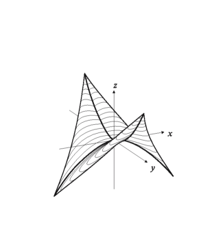
Figure 1. The hyperbolic hedgehog $\Sigma_{h}$ from [MM1].

Conjecture 2.4.

The support function $h$ of the hedgehog from [MM1] is a one-homogeneous singular minimizer of a functional of the type (1), where $D_{F}$ consists exactly of the four cusps of $\Sigma_{h}$.

This would show that the geometric conditions on $D_{F}$ in Theorem 2.1 are optimal.

Remark 2.5.

The surface $\Sigma_{h}$ can be written as the union of two graphs, which makes writing the Euler-Lagrange equation on $\Sigma_{h}$ relatively simple. Using this observation we can show that it is possible to construct $F$ locally (in particular, in a small neighborhood of a cusp), with some tedious calculation. It seems challenging to construct $F$ globally, but so far we do not see a fundamental obstruction.

Remark 2.6.

The regularity of $h$ in the example from ([MM1]) is $C^{2}$. Smooth counterexamples to Alexandrov’s conjecture, with (a version of) $\Sigma_{h}$ as a special case, were later constructed by Panina [P].

3. Proof of Theorem 2.1

Choose $M_{0}$ large so that $D_{F}\subset B_{M_{0}}$, and let $M=\max\{M_{0},\,\|u\|_{L^{\infty}(B_{1})}\}$. By a standard approximation argument, to prove Theorem 2.1 it suffices to assume $u,\,F\in C^{\infty}$ and show that the modulus of continuity of $\nabla u$ in $B_{1/2}$ depends only on $M$, the sets $\{\mathcal{O}_{k}\}$, and the moduli of continuity of $D^{2}F$ in the sets $\{B_{M}\cap\mathcal{O}_{k}\}$ (see e.g. [CF]).

3.1. Preliminaries

We record some important preliminary results. Our argument is based on applying the following estimate of De Giorgi (the “weak Harnack inequality”) to various functions of $\nabla u$:

Proposition 3.1.

Assume that $v\geq 0$ is in $H^{1}(B_{1})$ and solves $\partial_{i}(a_{ij}(x)v_{j})\geq 0$, with $a_{ij}$ bounded measurable and $\lambda I\leq(a_{ij})\leq\lambda^{-1}I$ for some $\lambda>0$. Then for all $\mu>0$, there exists $\nu(\mu,\,n,\,\lambda)>0$ such that if

$$\frac{|\{v>0\}\cap B_{1}|}{|B_{1}|}\leq 1-\mu$$

then

$$\sup_{B_{1/2}}v\leq(1-\nu)\sup_{B_{1}}v.$$

To prove Proposition 3.1 apply the weak Harnack inequality for supersolutions (Theorem $8.18$ in [GT]) to $\sup_{B_{1}}v-v$.

We now discuss the types of functions of $\nabla u$ that Proposition 3.1 applies to. We denote the linearized Euler-Lagrange operator by $L_{F}$. That is,

$$L_{F}(v):=\text{div}(D^{2}F(\nabla u)\nabla v)=\partial_{i}(F_{ij}(\nabla u)v_{j}).$$

The key observation is that if $\eta$ is slightly concave in only one direction, then $\eta(\nabla u)$ is a subsolution of $L_{F}$ where $\nabla u$ avoids $D_{F}$. For $\Omega\subset\mathbb{R}^{n}$ let $\mathcal{N}_{\delta}(\Omega)$ denote the $\delta$-neighborhood of $\Omega$. We have:

Lemma 3.2.

Assume $\eta$ is a smooth function in a neighborhood of $\nabla u(B_{1})$. For any $\rho\in(0,\,1)$, there exists $\lambda(\rho,\,F,\,M,\,n)>0$ such that if $\nabla u(B_{1})\cap\{\eta>0\}\subset B_{M}\backslash\mathcal{N}_{\rho}(D_{F})$, and in $\nabla u(B_{1})\cap\{\eta>0\}$ the eigenvalues $\gamma_{1}\leq\gamma_{2}\leq...\leq\gamma_{n}$ of $D^{2}\eta$ satisfy $\gamma_{2}>0$ and $\gamma_{1}\geq-\lambda\gamma_{2}$, then

$$L_{F}(\eta_{+}(\nabla u))\geq 0.$$

Here $\eta_{+}:=\max\{\eta,\,0\}$.

Proof.

Using that $L_{F}(u_{k})=0$ we compute

$$L_{F}(\eta(\nabla u))=\text{div}(D^{2}F(\nabla u)\nabla(\eta(\nabla u)))=F_{ij}u_{jk}\eta_{kl}u_{li}.$$

At a fixed point $x_{0}\in\{\eta(\nabla u)>0\}$ choose coordinates so that $\eta_{kl}(\nabla u(x_{0}))=\gamma_{k}\delta_{kl}$. Summing over $l$ we obtain

$$L_{F}(\eta(\nabla u))(x_{0})=\sum_{k=1}^{n}\gamma_{k}\sum_{i,\,j=1}^{n}F_{ij}u_{ki}u_{kj}.$$

For some $m$ large depending on $\rho,\,F,\,M$ we have $\nabla u(B_{1})\cap\{\eta>0\}\subset\mathcal{O}_{m}.$ Since $\gamma_{1}\geq-\lambda\gamma_{2}$ in $\{\eta(\nabla u)>0\}$ we conclude that

$$\gamma_{2}^{-1}L_{F}(\eta(\nabla u))(x_{0})\geq m^{-1}\sum_{k=2}^{n}|\nabla u_{k}(x_{0})|^{2}-m\,\lambda|\nabla u_{1}(x_{0})|^{2}.$$

If $L_{F}(\eta(\nabla u))(x_{0})<0$ then the above inequality gives

$$(\lambda^{-1}m^{-2}-1)\sum_{(i,\,j)\neq(1,\,1)}u_{ij}^{2}(x_{0})<u_{11}^{2}(x_{0}).$$

On the other hand, the equation $F_{11}u_{11}=-F_{ij}u_{ij}|_{(i,\,j)\neq(1,\,1)}$ gives

$$u_{11}^{2}\leq C(n,\,m)\sum_{(i,\,j)\neq(1,\,1)}u_{ij}^{2}$$

in $\{\eta(\nabla u)>0\}$. The previous two inequalities contradict each other for $\lambda(n,\,m)$ small. ∎

In order to apply Proposition 3.1 and Lemma 3.2, we need $\nabla u$ to be close to $D_{F}$ in sets of positive measure. The alternative is that $u$ nearly solves a non-degenerate equation. To handle this situation we will also use a “flatness implies regularity” result for $u$:

Proposition 3.3.

Assume that $a_{ij}$ are smooth elliptic coefficients on $\mathbb{R}^{n}$ that satisfy $\lambda I\leq(a_{ij})\leq\lambda^{-1}I$ in $B_{\rho}(p)$ for some fixed $\lambda,\,\rho>0,\,p\in\mathbb{R}^{n}$. There exists $\epsilon>0$ depending on $\rho,\,n,\,\lambda$ and the modulus of continuity of $a_{ij}$ in $B_{\rho}(p)$ such that if $v\in C^{\infty}(B_{1})$ solves $a_{ij}(\nabla v)v_{ij}=0$ and

$$\|v-l_{p}\|_{L^{\infty}(B_{1})}\leq\epsilon$$

for some linear function $l_{p}$ with $\nabla l_{p}=p$, then

$$\nabla v(B_{1/2})\subset B_{\rho}(p).$$

Heuristically, $w:=\epsilon^{-1}(v-l_{p})$ solves $a_{ij}(p+\epsilon\nabla w)w_{ij}=0$ which is nearly a constant-coefficient equation for $\epsilon$ small. The idea of Proposition 3.3 is due to Savin [S], who treated equations with degeneracy in the Hessian of $v$. For a proof of the proposition as stated (with degeneracy in the gradient of $v$) see [CF].

An easy consequence of Proposition 3.3 is:

Lemma 3.4.

For any $\rho\in(0,\,1)$ there exist $\epsilon_{1},\,\mu_{1}(\rho,\,F,\,M,\,n)>0$ such that if

$$\frac{|\{\nabla u\in B_{\epsilon_{1}}(p)\}\cap B_{r}|}{|B_{r}|}\geq 1-\mu_{1}$$

for some $p\in B_{2M}\backslash\mathcal{N}_{2\rho}(D_{F})$ then

$$\nabla u(B_{r/2})\subset B_{\rho}(p).$$

Proof.

After taking $u\rightarrow r^{-1}u(rx)$ we may assume that $r=1$. Since $u$ solves $F_{ij}(\nabla u)u_{ij}=0$, by Proposition 3.3 there exists $\epsilon_{0}>0$ depending on $\rho,\,F,\,M,\,n$ such that if

$$\|u-l_{p}\|_{L^{\infty}(B_{1})}\leq\epsilon_{0},$$

for some linear function $l_{p}$ with $\nabla l_{p}=p$, then $\nabla u(B_{1/2})\subset B_{\rho}(p)$. The above inequality holds by standard embeddings if we take e.g. $\epsilon_{1}<c(n)\epsilon_{0}$ and take $\mu_{1}$ small depending on $M,\,n,\,\epsilon_{0}$. ∎

Our approach to Theorem 2.1 is to first show that as $r\rightarrow 0$, the sets $\nabla u(B_{r})$ localize to the convex hull of $D_{F}$, and then to show that if this set is two-dimensional, they localize to a point. We treat these two results separately in the following sub-sections, and then combine them.

3.2. Localization to the Convex Hull

Let $K_{F}$ denote the convex hull of $D_{F}$. In this subsection we show:

Proposition 3.5.

For any $\rho>0$, there exists $s(\rho,\,F,\,M,\,n)>0$ such that either $\nabla u(B_{s})\subset B_{\rho}(p)$ for some $p\in B_{2M}\backslash\mathcal{N}_{2\rho}(D_{F})$, or $\nabla u(B_{s})\subset\mathcal{N}_{4\rho}(K_{F})$.

In this subsection we call a constant universal if it depends only on $\rho,\,M,\,F,\,n$. Let $\beta$ be a smooth uniformly convex function on $\mathbb{R}^{n}$ such that

$$\mathcal{N}_{3\rho}(K_{F})\subset\{\beta\leq 0\}\subset\mathcal{N}_{4\rho}(K_{F}),$$

with $B_{2M}\subset\{\beta<\tilde{M}\}$ for some universal $\tilde{M}$. Let $\epsilon_{1},\,\mu_{1}>0$ be the universal constants from Lemma 3.4, corresponding to $\rho$.

Lemma 3.6.

There exists $\delta>0$ universal such that if $\sup_{B_{r}}\beta(\nabla u)>0$ and

$$\frac{|\{\nabla u\in B_{\epsilon_{1}}(p)\}\cap B_{r}|}{|B_{r}|}<1-\mu_{1}$$

for all $p\in B_{2M}\backslash\mathcal{N}_{2\rho}(D_{F})$, then

$$\sup_{B_{r/2}}\beta(\nabla u)\leq\sup_{B_{r}}\beta(\nabla u)-\delta.$$

Proof.

After taking $u\rightarrow r^{-1}u(rx)$ we may assume that $r=1$. Let $0<t:=\sup_{B_{1}}\beta(\nabla u)\leq\tilde{M}$. For any unit vector $e$ let $s_{e}:=\sup_{\{\beta<t\}}(p\cdot e)$. There is some universal $\delta_{0}>0$ (independent of $e$) such that for some $c_{e}\leq s_{e}-\delta_{0}$ we have

$$\text{diam}(\{p\cdot e\geq c_{e}\}\cap\{\beta<t\})<\epsilon_{1}$$

and that $D^{2}F$ has universal ellipticity constant in $\{p\cdot c_{e}>0\}$. By the hypotheses we may apply Proposition 3.1 to $v:=(u_{e}-c_{e})_{+}$ with $\mu=\mu_{1}$ to conclude that $u_{e}\leq(1-\nu_{1})s_{e}+\nu_{1}c_{e}\leq s_{e}-\nu_{1}\delta_{0}$ in $B_{1/2}$, with $\nu_{1}>0$ universal. (Here we use that the coefficients of $L_{F}$ have universal ellipticity constant in $\{v>0\}$; we can replace the coefficients by e.g. $\delta_{ij}$ in $\{v=0\}$ without changing the equation for $v$). Since $\cap_{e\in S^{n-1}}\{p\cdot e\leq s_{e}-\nu_{1}\delta_{0}\}\subset\{\beta<t-\delta\}$ for some universal $\delta>0$ the proof is complete. ∎

Proof of Proposition 3.5.

Apply the following algorithm for $k\geq 0$: if one of the hypotheses of Lemma 3.6 is not satisfied in $B_{2^{-k}}$, then stop. We either have $\nabla u(B_{2^{-k}})\subset\{\beta\leq 0\}\subset\mathcal{N}_{4\rho}(K_{F})$, or we can apply Lemma 3.4 to conclude $\nabla u(B_{2^{-k-1}})\subset B_{\rho}(p)$ for some $p\in B_{2M}\backslash\mathcal{N}_{2\rho}(D_{F})$. Otherwise, we apply Lemma 3.6. The algorithm terminates after at most $k_{0}$ steps with $\tilde{M}-k_{0}\delta\leq 0$. ∎

3.3. Localization Beyond the Convex Hull

In this subsection we show that if $\nabla u(B_{1})$ is sufficiently close to a two-dimensional affine subspace, then as $r\rightarrow 0$ the gradients $\nabla u(B_{r})$ localize to a connected component of $D_{F}$.

Let $(p,\,q)\in\mathbb{R}^{n}$ with $p\in\mathbb{R}^{2}$ and $q\in\mathbb{R}^{n-2}$, and assume that $D_{F}\subset\{q=0\}$. Let $8\rho_{0}$ be the smallest distance between a pair of points in $D_{F}$. In this subsection we call constants depending on $\rho_{0},\,F,\,M,\,n$ universal.

Proposition 3.7.

There exist $\sigma_{0},\,r_{0}>0$ universal such that if $\nabla u(B_{1})\subset\{|q|<\sigma_{0}\}$ then either $\nabla u(B_{r_{0}})\subset B_{\rho_{0}}(p)$ for some $p\in B_{2M}\backslash\mathcal{N}_{2\rho_{0}}(D_{F})$ or $\nabla u(B_{r_{0}})\subset\mathcal{N}_{3\rho_{0}}(D_{F})$.

In particular, since $\nabla u$ is (qualitatively) continuous the set $\nabla u(B_{r_{0}})$ is connected, so it is contained in a ball with at most one point of $D_{F}$, and is a distance at least $\rho_{0}$ from the remaining points in $D_{F}$.

The idea is to localize the gradients using the level sets of non-convex functions of $\nabla u$. Let $\epsilon_{1},\,\mu_{1}>0$ be the (universal) constants from Lemma 3.4 with $\rho=\rho_{0}$. We assume by taking $\epsilon_{1}$ smaller if necessary that $\epsilon_{1}\leq\rho_{0}$. Let $\lambda_{1}$ be the constant from Lemma 3.2 with $\rho=\rho_{0}$. Finally, let $\nu_{1}$ be the constant from Proposition 3.1 corresponding to $\mu=\mu_{1}$ and the ellipticity constants of $D^{2}F$ in $B_{2M}\backslash\mathcal{N}_{\rho_{0}}(D_{F})$. The following lemma says that when the gradient image is sufficiently close to $\{q=0\}$, we can “chop” at its projection to $\{q=0\}$ with circles (see Figure 2):

Lemma 3.8.

Let $(p_{0},\,0)\in B_{2M}\backslash\mathcal{N}_{2\rho_{0}}(D_{F})$. There exist $\sigma_{0},\,\delta_{0}>0$ universal such that if $\nabla u(B_{r})\subset\{|q|<\sigma_{0}\}\cap\{|p-p_{0}|\geq\epsilon_{1}/4\}$ and

$$\frac{|\{\nabla u\in B_{\epsilon_{1}}(p_{0},\,0)\}\cap B_{r}|}{|B_{r}|}<1-\mu_{1},$$

then

$$\nabla u(B_{r/2})\subset\{|p-p_{0}|\geq\epsilon_{1}/4+\delta_{0}\}.$$

Proof.

We may assume that $r=1$ after a Lipschitz rescaling. Define

$$\eta_{A}(p,\,q):=e^{A^{2}|q|^{2}/2-A|p|},\quad\eta_{A,\,p_{0}}:=\eta_{A}(p-p_{0},\,q)-e^{-A\epsilon_{1}/2}.$$

In an appropriate system of coordinates we have in $\{|q|<A^{-3}\}$ that

$$(A^{2}\eta_{A})^{-1}D^{2}\eta_{A}=\text{diag}(-(A|p|)^{-1},\,1,\,...,\,1)+O(A^{-2}),$$

and that $\{\eta_{A}>e^{-A\epsilon_{1}/2}\}\subset\{|p|<\epsilon_{1}/2+A^{-5}\}$. Then by our first hypothesis, for $A$ large universal and $\sigma_{0}<A^{-3}$ we have $\nabla u(B_{1})\cap\{\eta_{A,\,p_{0}}>0\}\subset B_{M}\cap B_{\epsilon_{1}}(p_{0},\,0)\subset B_{M}\backslash\mathcal{N}_{\rho_{0}}(D_{F})$, and that the eigenvalues $\gamma_{1}\leq...\leq\gamma_{n}$ of $D^{2}\eta_{A,\,p_{0}}$ satisfy $\gamma_{2}>0$ and $\gamma_{1}>-\lambda_{1}\gamma_{2}$ in $\nabla u(B_{1})\cap\{\eta_{A,\,p_{0}}>0\}$. We conclude using Lemma 3.2 that the function $v_{p_{0}}:=(\eta_{A,\,p_{0}})_{+}(\nabla u)$ satisfies $L_{F}(v_{p_{0}})\geq 0$. By our second hypothesis we can apply Proposition 3.1 to $v_{p_{0}}$. In the extreme case that $\sigma_{0}=0$, Proposition 3.1 gives

$$\nabla u(B_{1/2})\subset\{\eta_{A,\,p_{0}}<(1-\nu_{1})(e^{-A\epsilon_{1}/4}-e^{-A\epsilon_{1}/2})\}\subset\{|p-p_{0}|\geq\epsilon_{1}/4+2\delta_{0}\}$$

for some $\delta_{0}>0$ universal. By continuity we have the same inclusion with $2\delta_{0}$ replaced by $\delta_{0}$ for sufficiently small $\sigma_{0}<A^{-3}$, completing the proof. ∎

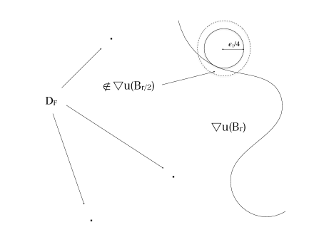
Figure 2. If $\nabla u(B_{r})$ is “nearly $2D$” we can chop its projection to $\{q=0\}$ with circles. The picture illustrates the case $n=2$.

We can now prove Proposition 3.7.

Proof of Proposition 3.7:.

Take $\sigma_{0}$ as in Lemma 3.8, and apply the following algorithm for $k\geq 0$: If

$$\frac{|\{\nabla u\in B_{\epsilon_{1}}(p_{0},\,0)\}\cap B_{2^{-k}}|}{|B_{2^{-k}}|}\geq 1-\mu_{1}$$

for some $(p_{0},\,0)\in B_{2M}\backslash\mathcal{N}_{2\rho_{0}}(D_{F})$, then stop. We have by Lemma 3.4 that $\nabla u(B_{2^{-k-1}})\subset B_{\rho_{0}}(p_{0},\,0)$. If not, apply Lemma 3.8 to conclude that

$$\nabla u(B_{2^{-k-1}})\subset\{|p-p_{0}|\geq\epsilon_{1}/4+\delta_{0}\}$$

for all $(p_{0},\,0)\in B_{2M}\backslash\mathcal{N}_{2\rho_{0}}(D_{F})$ such that $\nabla u(B_{2^{-k}})\subset\{|p-p_{0}|\geq\epsilon_{1}/4\}$. If at this point we can conclude that $\nabla u(B_{2^{-k-1}})\subset\mathcal{N}_{3\rho_{0}}(D_{F})$, then stop.

To show that this algorithm terminates after a universal number of steps, we use a simple covering argument. Let $\mathcal{S}_{k}$ be the projections of the sets $\nabla u(B_{2^{-k}})$ to $\{q=0\}$. Take a finite number of lines $\{l_{i}\}$ in $\{q=0\}$ that avoid $\mathcal{N}_{2\rho_{0}}(D_{F})$, whose $\epsilon_{1}/4$ neighborhoods cover $B_{2M}\backslash\mathcal{N}_{2\rho_{0}}(D_{F})\cap\{q=0\}$. For each $l_{i}$ take a universal number $J+1$ of two-dimensional balls $\{B_{ij}:=B_{\epsilon_{1}/4}(p_{ij})\}_{j=1}^{J+1}$ in $\{q=0\}$ that cover $B_{2M}\cap l_{i}\cap\{q=0\}$, with centers $p_{ij}\in B_{2M}\cap l_{i}\cap\{q=0\}$ on $l_{i}$ such that $|p_{i,\,j+1}-p_{ij}|\leq\delta_{0}$ for $j=1,\,...,\,J$. Since $\mathcal{S}_{0}\subset B_{M}$ we can arrange that $B_{i1}\cap\mathcal{S}_{0}=\emptyset$ for all $i$. By induction, if the algorithm doesn’t terminate after $k$ steps, then $\mathcal{S}_{k}$ has empty intersection with the convex hull of $B_{i1}$ and $B_{i,\,k+1}$, for each $i$. In particular, after $J$ steps we have that $\mathcal{S}_{J}\subset\mathcal{N}_{2\rho_{0}}(D_{F})$, and the proof is complete up to replacing $\sigma_{0}$ with $\min\{\sigma_{0},\,\rho_{0}\}$. ∎

3.4. Proof of Theorem 2.1

We are now in position to prove Theorem 2.1. We call constants depending on $F,\,M,\,n$ universal.

Proof.

For any $\epsilon>0$ we will show that there is some $\delta(\epsilon,\,F,\,M,\,n)>0$ such that $\nabla u(B_{\delta})$ is contained in a ball of radius $\epsilon$.

Take $\sigma_{0}$ to be the constant from Proposition 3.7. Applying Proposition 3.5 with $\rho=\sigma_{0}/4$ we obtain $s_{0}>0$ universal such that either $\nabla u(B_{s_{0}})\subset B_{\sigma_{0}/4}(p)$ for some $p\in B_{2M}\backslash\mathcal{N}_{\sigma_{0}/2}(D_{F})$, or $\nabla u(B_{s_{0}})\subset\mathcal{N}_{\sigma_{0}}(K_{F})$. In the latter case, apply Proposition 3.7 to $s_{0}^{-1}u(s_{0}x)$ to conclude for some $r_{0}>0$ universal that either $\nabla u(B_{r_{0}s_{0}})\subset B_{\rho_{0}}(p)$ for some $p\in B_{2M}\backslash\mathcal{N}_{2\rho_{0}}(D_{F})$ or $\nabla u(B_{r_{0}s_{0}})\subset\mathcal{N}_{3\rho_{0}}(D_{F})$.

In all cases, $\nabla u(B_{r_{0}s_{0}})$ is contained in a ball $\mathcal{B}$ that has at most one point of $D_{F}$ and is a positive universal distance from the remaining points of $D_{F}$. Thus, after restricting our attention to $\tilde{u}=(r_{0}s_{0})^{-1}u(r_{0}s_{0}x)$ we may assume that $D_{F}$ contains at most one point (indeed, we can modify $F$ outside of $\mathcal{B}$ without changing that $\tilde{u}$ is a minimizer). Applying Proposition 3.5 to $\tilde{u}$ with $\rho=\epsilon/4$ completes the proof. ∎

4. Proof of Theorem 2.3

In this section we construct the examples from Theorem 2.3. Here and below we let $k\geq 1$, and $q=(q_{1},\,q_{2}),\,y=(y_{1},\,y_{2})\in\mathbb{R}^{2k+2}$ with $q_{i},\,y_{i}\in\mathbb{R}^{k+1},\,i=1,\,2.$ We will reduce the problem to making a certain one-dimensional construction using the symmetries of $w$.

4.1. Reduction to Two Dimensions

We first reduce Theorem 2.3 to a problem in two dimensions. Let $v$ be the one-homogeneous function on $\mathbb{R}^{2}$ given by

$$v(x_{1},\,x_{2}):=\frac{1}{\sqrt{2}}\frac{x_{2}^{2}-x_{1}^{2}}{|x|}.$$

We claim it suffices to construct a $C^{1}$, uniformly convex function $G(p_{1},\,p_{2})$ on $\mathbb{R}^{2}$ that is smooth away from $D_{G}=\sqrt{2}\,S^{1}\cap\{p_{1}^{2}=p_{2}^{2}\}$, such that $G$ is invariant under reflection over the axes and over the lines $\{p_{1}=\pm p_{2}\}$ (that is, $G(p_{1},\,p_{2})=G(-p_{1},\,p_{2})=G(p_{2},\,p_{1})$) and furthermore

(5) $$\text{tr}(D^{2}G(\nabla v)\,D^{2}v)+k\,\nabla G(\nabla v)\cdot\left(\frac{1}{x_{1}},\,\frac{1}{x_{2}}\right)=0$$

for $x$ in the positive quadrant. Indeed, if we manage to do this, note that by the symmetries of $G$ and $v$, each term on the left is smooth away from $\{x_{1}^{2}=x_{2}^{2}\}$, where $\nabla v$ maps to $D_{G}$. If we then take $F(q)=G(|q_{1}|,\,|q_{2}|)$ we obtain a $C^{1}$, uniformly convex function on $\mathbb{R}^{2k+2}$ that is smooth away from $D_{F}=\sqrt{2}\,S^{2k+1}\cap\{|q_{1}|^{2}=|q_{2}|^{2}\}$. Using that $w(y)=v(|y_{1}|,\,|y_{2}|)$ we compute

$$\text{tr}(D^{2}F(\nabla w)\,D^{2}w)(y) =\text{tr}(D^{2}G(\nabla v)\,D^{2}v)(|y_{1}|,\,|y_{2}|)$$

$$+k\,\nabla G(\nabla v(|y_{1}|,\,|y_{2}|))\cdot\left(\frac{1}{|y_{1}|},\,\frac{1}{|y_{2}|}\right)$$

$$=0$$

classically away from the cone $\{|y_{1}|^{2}=|y_{2}|^{2}\}$. Here we used that $v_{1}<0$ and $v_{2}>0$ in the positive quadrant. It is not hard to show that the equation $\text{div}(\nabla F(\nabla w))=0$ holds in the weak sense in $B_{1}$ by integrating away from a thin cone containing $\{|y_{1}|^{2}=|y_{2}|^{2}\}$ and a small ball around the origin, using the $C^{1}$ regularity of $F$ and the one-homogeneity of $w$, and taking a limit.

4.2. Reduction to One Dimension

We now use that $\Sigma_{v}:=\nabla v(S^{1})$ is one-dimensional and an extension lemma to reduce our problem to one dimension. The set $\nabla v(S^{1}\cap\{x_{2}\geq|x_{1}|\})$ can be written as a graph $\Gamma_{1}:=\{(p_{1},\,\varphi(p_{1}))\}$ with $p_{1}\in[-1,\,1]$, where $\varphi\in C^{\infty}(-1,\,1)\cap C^{1}([-1,\,1])$ is even, uniformly convex, and separates from the lines $p_{2}=\pm p_{1}$ like $\text{dist.}^{3/2}$ at the endpoints. See the Appendix for a justification of these properties, as well as an expansion of $\varphi$ near the endpoints. The set $\Sigma_{v}$ consists of four rotations of $\Gamma_{1}$ by $\pi/2$ (see Figure 3). Let $S:=\sqrt{2}\,S^{1}\cap\{p_{1}^{2}=p_{2}^{2}\}$, and let $\Sigma_{0}:=\Sigma_{v}\backslash S,\,\Gamma_{0}:=\Gamma_{1}\backslash S$. We will use the following important extension lemma:

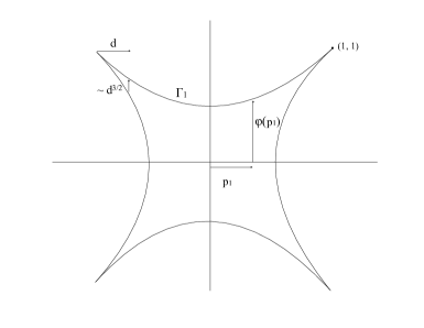
Figure 3. The set $\Sigma_{v}$ consists of four congruent curves separating from the lines $p_{2}=\pm p_{1}$ like $\text{dist}^{3/2}.$

Lemma 4.1.

Assume that $g:\Sigma_{v}\rightarrow\mathbb{R}$ and ${\bf v}:\Sigma_{v}\rightarrow\mathbb{R}^{2}$ are smooth on $\Sigma_{0}$ and continuous on $\Sigma_{v}$, and satisfy the condition

(6) $$g(\tilde{p})-g(p)-{\bf v}(p)\cdot(\tilde{p}-p)\geq\gamma|\tilde{p}-p|^{2}$$

for some $\gamma>0$ and all $\tilde{p},\,p\in\Sigma_{v}$. Then there exists a $C^{1}$, uniformly convex function $G$ on $\mathbb{R}^{2}$ with $G\in C^{\infty}(\mathbb{R}^{2}\backslash S)$, such that $G=g$ and $\nabla G={\bf v}$ on $\Sigma_{v}$.

We delay the proof of Lemma 4.1 to the Appendix, and proceed with the reduction. We claim that it suffices to construct even functions $f,\,h\in C^{\infty}(-1,\,1)\cap C^{1}([-1,\,1])$ such that

(7) $$h=\frac{1}{1+2k}\left(\frac{f^{\prime\prime}}{\varphi^{\prime\prime}}+k\frac{f^{\prime}}{\varphi^{\prime}}\right)$$

on $(-1,\,1)$, and furthermore the pair $(g,\,{\bf v})$ defined on $\Sigma_{v}$ by

(8) $$g(s,\,\varphi(s)):=f(s),\quad{\bf v}(s,\,\varphi(s)):=(f^{\prime}(s)-h(s)\varphi^{\prime}(s),\,h(s))$$

on $\Gamma_{1}$ and extended by reflection over the lines $p_{2}=\pm p_{1}$, satisfies the conditions of Lemma 4.1 for some $\gamma>0$. Indeed, if this is accomplished, then the extension $G$ from Lemma 4.1 satisfies the Euler-Lagrange equation (5). To see this, let $\nu$ be the upward unit normal to $\Gamma_{0}$. By the one-homogeneity of $v$ we have

$$x=\nu(\nabla v(x))=\frac{(-\varphi^{\prime},\,1)}{\sqrt{1+\varphi^{\prime 2}}}$$

for $x\in S^{1}\cap\{x_{2}>|x_{1}|\}$. Differentiating in $x$ gives

$$D^{2}v(x)=\frac{1}{\kappa}\tau\otimes\tau=-\frac{(1+\varphi^{\prime 2})^{3/2}}{\varphi^{\prime\prime}}\tau\otimes\tau$$

where $\tau$ is the unit tangent vector to $\Gamma_{0}$ at $\nabla v(x)$ (also the unit tangent to $S^{1}$ at $x$) and $\kappa$ is the (signed) curvature of $\Gamma_{0}$. Finally, by (8) we have

(9) $$G(s,\,\varphi(s))=f(s),\quad G_{2}(s,\,\varphi(s))=h(s)$$

on $\Gamma_{0}$. Differentiating the first relation in (9) twice we obtain

$$\nabla G=(f^{\prime}-h\varphi^{\prime},\,h),\quad\tau^{T}\cdot D^{2}G\cdot\tau=\frac{f^{\prime\prime}-h\varphi^{\prime\prime}}{1+\varphi^{\prime 2}}$$

on $\Gamma_{0}$. Putting these together gives the equivalence of (5) and (7). Finally, since $(G,\,\nabla G)$ has the desired symmetries on $\Sigma_{v}$, we can arrange that $G$ has the desired symmetries globally by taking the average of its reflections.

Remark 4.2.

One can compute the Euler-Lagrange equation (7) directly in $\mathbb{R}^{2k+2}$ using the geometry of $\Sigma_{w}:=\nabla w(S^{2k+1})$, without much trouble. Using the one-homogeneity of $w$ we see as above that the equation reduces to $\text{tr}((II)^{-1}(q)\,D_{T}^{2}F(q))=0$ on $\Sigma_{w}$, where $II$ is the second fundamental form of $\Sigma_{w}$ and $T$ is the tangent hyperplane to $\Sigma_{w}$. Since $\Sigma_{w}$ is obtained by taking rotations of $\Gamma_{1}$, it is tangent on one side to second order to a sphere of radius $\varphi\sqrt{1+\varphi^{\prime 2}}$ and on the other side to second order to a sphere of radius $\frac{s}{\varphi^{\prime}}\sqrt{1+\varphi^{\prime 2}}$. It thus has one principal curvature $-\varphi^{\prime\prime}\,(1+\varphi^{\prime 2})^{-3/2}$, $k$ principal curvatures $\frac{1}{\varphi\,\sqrt{1+\varphi^{\prime 2}}}$ from rotating around the $p_{1}$ axis, and $k$ principal curvatures $-\frac{\varphi^{\prime}}{s\sqrt{1+\varphi^{\prime 2}}}$ from rotating around the $p_{2}$ axis. The eigenvalues of $D^{2}F$ corresponding to these directions are $\frac{f^{\prime\prime}-h\varphi^{\prime\prime}}{1+\varphi^{\prime 2}},\,\frac{h}{\varphi}$ and $\frac{f^{\prime}-h\varphi^{\prime}}{s}$, where the latter two come from rotations. Putting these together in the original Euler-Lagrange equation $\text{tr}((II)^{-1}(q)\,D_{T}^{2}F(q))=0$ we recover (7).

4.3. The One-Dimensional Construction

We now construct $f$ and $h$. The Euler-Lagrange equation (7) determines $h$ through our choice of $f$, so there is only one function to construct. It is convenient to do this by taking

(10) $$f^{\prime\prime}(s):=\eta(s)\varphi^{\prime\prime}(s),\,f^{\prime}(0)=0$$

for some positive $\eta\in C^{\infty}(-1,\,1)\cap C([-1,\,1])$. Fix $0<\delta<<1$. We choose $\eta$ satisfying the following conditions:

1. $\eta$ is even, concave, and $\eta(1)=1/2$,

2. $\eta\geq\min\left\{1,\,\frac{1}{2}(1+\delta^{-1/2}(1-s)^{1/2})\right\}$,

3. $\eta\equiv 1+\mu$ on $[0,\,1-\delta]$ for some $\mu>0$,

4. $\int_{0}^{1}\eta(s)\varphi^{\prime\prime}(s)\,ds=1$.

Since $\int_{0}^{1}\varphi^{\prime\prime}(s)\,ds=1$, it is clear that $\mu\rightarrow 0$ as we take $\delta\rightarrow 0$. We will show below that for any such choice of $\eta$ with $\delta$ sufficiently small, the pair $(g,\,{\bf v})$ defined by (8) satisfies the hypotheses of Lemma 4.1.

Continuity Condition: The condition that ${\bf v}$ is continuous on $\Sigma_{v}$ and invariant under reflection over the diagonal is that

(11) $$(f^{\prime}-h\varphi^{\prime},\,h)(1)\text{ is parallel to }(1,\,1).$$

This follows from (7), using that $\eta(1)=1/2$ and $f^{\prime}(1)=\varphi^{\prime}(1)=1$.

Convexity Condition Along Top Graph. We check the convexity condition (6) on $\Gamma_{1}\cap\{p_{1}\geq 0\}$. Take $\tilde{p}=(y,\,\varphi(y))$ and $p=(x,\,\varphi(x))$ for some $x,\,y\in[0,\,1]$. The quantity of interest is

$$g(y,\,\varphi(y)) -g(x,\,\varphi(x))-{\bf v}(x,\,\varphi(x))\cdot(y-x,\,\varphi(y)-\varphi(x))$$

$$=[f(y)-f(x)-f^{\prime}(x)(y-x)]-h(x)[\varphi(y)-\varphi(x)-\varphi^{\prime}(x)(y-x)]$$

$$=\int_{x}^{y}f^{\prime\prime}(x)(y-s)\,ds-h(x)\int_{x}^{y}\varphi^{\prime\prime}(s)(y-s)\,ds$$

$$=\left(\int_{x}^{y}\varphi^{\prime\prime}(s)(y-s)\,ds\right)H(x,\,y),$$

where

$$H(x,\,y)=\int_{x}^{y}(\eta-1/2)(s)d\mu_{y}(s)-\frac{1}{1+2k}(\eta-1/2)(x)-\frac{k}{1+2k}\frac{f^{\prime}-\varphi^{\prime}}{\varphi^{\prime}}(x),$$

and $d\mu_{y}$ is the probability density

$$d\mu_{y}:=\frac{\varphi^{\prime\prime}(s)(y-s)\,ds}{\int_{x}^{y}\varphi^{\prime\prime}(t)(y-t)\,dt}$$

on the interval from $x$ to $y$. We claim that

(12) $$H(x,\,y)\geq c_{0}\,\max\{(1-x)^{1/2},\,(1-y)^{1/2}\}$$

for some $c_{0}>0$ independent of $x,\,y\in[0,\,1]$. The desired inequality (6) then follows because

$$\frac{1}{(y-x)^{2}}\int_{x}^{y}\varphi^{\prime\prime}(s)(y-s)\,ds\geq c\,\min\{(1-x)^{-1/2},\,(1-y)^{-1/2}\}$$

for some $c>0$, using that $\varphi^{\prime\prime}$ is positive, increasing on $[0,\,1)$, and has the expansion $\varphi^{\prime\prime}(s)=\sqrt{\frac{2}{3}}(1-s)^{-1/2}+O(1)$ near $s=1$ (see Appendix). To show (12) we check several cases. Below, $c_{1},\,c_{2}$ always denote universal positive constants which may change from line to line.

In the case that $x,\,y\leq 1-\delta$ it is obvious that $H(x,\,y)\geq c_{0}>0$ since $\eta-1/2>1/2$ is constant on $[0,\,1-\delta]$ and $f^{\prime}-\varphi^{\prime}=\mu\varphi^{\prime}$ with $\mu$ small.

The next simplest case is that $y<x$ and $x>1-\delta$. Using that $\eta$ is decreasing, that $f^{\prime}\leq 1$, and the expansion of $\varphi^{\prime}(s)$ near $s=1$ (see Appendix) we have

$$H(x,\,y)\geq\frac{2}{3}\int_{x}^{y}(\eta-1/2)(s)d\mu_{y}(s)-c_{1}\,(1-x)^{1/2}.$$

It is elementary to check that the mass of $d\mu_{y}$ in the left half of the interval $[y,\,x]$ is at least $c_{2}>0$ independent of $y$ using the properties of $\varphi$. Since $\eta$ is decreasing and concave we conclude that

$$H(x,\,y)\geq\frac{1}{3}c_{2}\,(\eta-1/2)(y)-c_{1}\,(1-x)^{1/2}\geq c_{0}(1-y)^{1/2}$$

using definition of $\eta$ and that $\delta$ is small.

The most delicate case is that $x<y$ and $y>1-\delta$. By the expansion of $\varphi(s)$ near $s=1$ we may choose $\delta$ so small that $d\mu_{y}$ is decreasing on $[1-2\delta,\,y]$, independent of $y>1-\delta$ (see Appendix). We first claim that

$$\int_{x}^{y}(\eta-1/2)(s)d\mu_{y}(s)\geq\frac{1}{2}(\eta-1/2)(x).$$

If $x<1-2\delta$ then since most of the weight of $d\mu_{y}$ on $[x,\,y]$ is to the left of $1-\delta$ the inequality is obvious. When $x\geq 1-2\delta$, since both the weight $d\mu_{y}$ and $\eta$ are decreasing on $[x,\,y]$, the average of $\eta-1/2$ decreases if we redistribute the weight $d\mu_{y}$ evenly, and the concavity of $\eta$ gives the result. We conclude that

$$H(x,\,y)\geq\frac{1}{6}(\eta-1/2)(x)-\frac{f^{\prime}-\varphi^{\prime}}{2\varphi^{\prime}}(x).$$

If $x\leq 1-\delta$ we have $f^{\prime}-\varphi^{\prime}=\mu\varphi^{\prime}$ and $\eta-1/2>1/2$ so $H(x,\,y)\geq c_{0}>0$. If $x>1-\delta$ we argue as in the case $y<x$ that

$$H(x,\,y)\geq\frac{1}{12}\delta^{-1/2}(1-x)^{1/2}-c_{1}(1-x)^{1/2}>(1-x)^{1/2}$$

for $\delta$ small, and inequality (12) follows.

Global Convexity Condition. Finally, for the convexity condition (6) to hold on all of $\Sigma_{v}$, it suffices by reflection symmetry to show that

(13) $${\bf v}(s,\,\varphi(s))\cdot(1,\,0)\geq c_{0}s,\quad{\bf v}(s,\,\varphi(s))\cdot(-1,\,1)\geq c_{0}(\varphi(s)-s)$$

for some fixed $c_{0}>0$ and all $s\in[0,\,1]$.

For $\delta$ small it is straightforward to show that $h<3/4$, so $f^{\prime}-h\varphi^{\prime}\geq c_{0}\varphi^{\prime}$, and the first inequality in (13) follows.

For the second we compute

$$(1+2k){\bf v}\cdot(-1,\,1) =(1+2k)[(1+\varphi^{\prime})h-f^{\prime}]$$

$$=(1+\varphi^{\prime})\eta+[k(1+1/\varphi^{\prime})-(1+2k)]f^{\prime}$$

$$=(1+\varphi^{\prime})\eta+[k(1/\varphi^{\prime}-1)-1]f^{\prime}$$

$$\geq(1+\varphi^{\prime})\eta-f^{\prime}.$$

When $0\leq s\leq 1-\delta$ this quantity is larger than $1$ by the definition of $\eta$. For $s\geq 1-\delta$ we use the expansion $\varphi^{\prime}=1-c_{1}\,(1-s)^{1/2}+O(1-s)$ (see Appendix) and that $f^{\prime}\leq 1$ to get

$$(1+\varphi^{\prime})\eta-f^{\prime} \geq(2-c_{1}(1-s)^{1/2})\eta-1+O(1-s)$$

$$=(2\eta-1)-c_{1}\eta(1-s)^{1/2}+O(1-s)$$

$$\geq(\delta^{-1/2}-2c_{1})(1-s)^{1/2}+O(1-s)$$

$$\geq\frac{1}{2}\delta^{-1/2}(1-s)^{1/2}$$

for $\delta$ small. We conclude that

$${\bf v}\cdot(-1,\,1)\geq c_{0}\min\{1,\,\delta^{-1/2}(1-s)^{1/2}\}.$$

Since $\varphi(s)-s\leq c_{2}(1-s)^{3/2}$ for some $c_{2}>0$, this confirms (13).

4.4. Proof of Theorem 2.3

Proof.

Choose $\eta$ as in the previous subsection. Then the pair $(g,\,{\bf v})$ determined by $\eta$ through the relations (10), (7), and (8) satisfies the hypotheses of Lemma 4.1. We showed above that the extension $G$ then satisfies the Euler-Lagrange equation (5) and can be chosen symmetric over the axes and over the lines $p_{1}=\pm p_{2}$, and that the result follows by taking $F(q)=G(|q_{1}|,\,|q_{2}|)$. ∎

Remark 4.3.

If we choose $\eta-1/2$ to be a multiple of $(1-s)^{1/2}$ near $s=1$, then a straightforward computation shows that the $2k+1$ second derivatives of $F$ in directions tangent to $\Sigma_{w}$ are bounded, and the only second derivative of $F$ that tends to $\infty$ is the one normal to $\Sigma_{w}$. The regularity of $F$ near $D_{F}$ is in fact $C^{1,\,\frac{1}{3}}$, by the computation that confirms the second inequality in (13).

5. Appendix

In the Appendix we record some properties of $\varphi$, and we prove the extension result Lemma 4.1.

5.1. Properties of $\varphi$

We recall from [MS] that if we parametrize $\Gamma_{1}$ by the angle $\theta\in[\pi/4,\,3\pi/4]$ of its upward unit normal $\nu$, then its curvature is given by $\kappa=\frac{\sqrt{2}}{3}\sec(2\theta)$. It follows easily that $\varphi$ is smooth, even, and uniformly convex on $(-1,\,1)$, and $\varphi^{\prime\prime}$ is increasing on $[0,\,1)$. We recall also the expansion

$$\varphi\left(-1+\frac{3}{2}\theta^{2}+\theta^{3}+O(\theta^{4})\right)=1-\frac{3}{2}\theta^{2}+\theta^{3}+O(\theta^{4})$$

from [MS]. By differentiating implicitly and using that $\varphi$ is even we obtain near $s=1$ the expansions

$$\varphi^{\prime}(s)=1-2\sqrt{\frac{2}{3}}(1-s)^{1/2}+O(1-s)$$

$$\varphi^{\prime\prime}(s)=\sqrt{\frac{2}{3}}(1-s)^{-1/2}+O(1)$$

$$\varphi^{\prime\prime\prime}(s)=\frac{1}{2}\sqrt{\frac{2}{3}}(1-s)^{-3/2}+O((1-s)^{-1}).$$

In particular, for $0<s<y$ the derivative of the weight $\varphi^{\prime\prime}(s)(y-s)$ is bounded above by $\varphi^{\prime\prime\prime}(s)(1-s)-\varphi^{\prime\prime}(s)=-\frac{1}{2}\sqrt{\frac{2}{3}}(1-s)^{-1/2}+O(1)<0$ for $s$ close to $1$.

5.2. Proof of Extension Lemma

We now prove Lemma 4.1. Our strategy is to first construct $G$ in a set containing a neighborhood of every point on $\Sigma_{0}$. We then apply a global $C^{1}$ extension result to this local extension. To complete the construction we use a mollification and gluing procedure.

5.2.1. Local Extension

Lemma 5.1.

There exists an open set $\mathcal{O}$ containing a neighborhood of each point on $\Sigma_{0}$ and a function $G_{0}\in C^{\infty}(\mathcal{O})$ such that $G_{0}=g$ and $\nabla G_{0}={\bf v}$ on $\Sigma_{0}$, and furthermore

(14) $$G_{0}(\tilde{p})-G_{0}(p)-\nabla G_{0}(p)\cdot(\tilde{p}-p)\geq\frac{\gamma}{2}|\tilde{p}-p|^{2}$$

for all $p,\,\tilde{p}\in\mathcal{O}$.

Proof.

The squared distance function $d_{\Sigma_{v}}^{2}$ from $\Sigma_{v}$ is smooth in a neighborhood of each point on $\Sigma_{0}$, as is the projection $\pi_{\Sigma_{v}}$ to $\Sigma_{v}$. Let $\tau$ be a unit tangent vector field to $\Sigma_{v}$ in a neighborhood of a point on $\Sigma_{0}$, and $\nu$ a unit normal vector field. Then $D^{2}(d_{\Sigma_{v}}^{2}/2)$ projects in the normal direction $\nu$ on $\Sigma_{0}$. See e.g. [AS] for proofs of these properties.

Let $A>0$ be a smooth function on $\Sigma_{0}$ to be chosen, and define

$$G_{0}(x):=g(\pi_{\Sigma_{v}}(x))+{\bf v}(\pi_{\Sigma_{v}}(x))\cdot(x-\pi_{\Sigma_{v}}(x))+A(\pi_{\Sigma_{v}}(x))d_{\Sigma_{v}}^{2}.$$

It is elementary to check using (6) that $\nabla_{\Sigma_{0}}g$ is the tangential component of ${\bf v}$ on $\Sigma_{0}$, and as a consequence that $G_{0}=g,\,\nabla G_{0}={\bf v}$ on $\Sigma_{0}$. Furthermore, it follows from (6) that $(G_{0})_{\tau\tau}\geq 2\gamma$ on $\Sigma_{0}$. Since $D^{2}(A(\pi_{\Sigma_{v}}(x))d_{\Sigma_{v}}^{2})$ is $2A$ times the matrix that projects in the direction $\nu$ on $\Sigma_{0}$, we have that $(G_{0})_{\nu\nu}=2A$ on $\Sigma_{0}$, and that $(G_{0})_{\tau\nu}$ on $\Sigma_{0}$ depends only on $g,\,{\bf v}$, and the geometry of $\Sigma_{0}$ (in particular, not on $A$). By choosing $A(p)$ sufficiently large depending on $\gamma$ and these quantities (and perhaps going to $\infty$ as $p\rightarrow S$), we have that

(15) $$D^{2}G_{0}\geq\frac{3}{2}\gamma I$$

on $\Sigma_{0}$. In particular, (14) holds in a small neighborhood of each point on $\Sigma_{0}$.

Now, for $\delta,\,\sigma>0$ let $S_{\delta}$ be the closed $\delta$-neighborhood of $S$, and let $\Sigma_{\sigma}$ be the open $\sigma$-neighborhood of $\Sigma_{v}$. By (6), (15), and continuity, for each $\delta>0$ there exists $\sigma(\delta)>0$ small and an open set $O_{\delta}$ containing $\Sigma_{\sigma(\delta)}\backslash S_{\delta}$ and a neighborhood of each point in $\Sigma_{0}$, such that (14) holds for all $p,\,\tilde{p}\in O_{\delta}$ such that at least one of $p,\,\tilde{p}$ is in $\Sigma_{\sigma(\delta)}\backslash S_{\delta}$. For $\delta=1/k$ we may choose $\sigma(1/k)$ and $O_{1/k}$ such that $\Sigma_{\sigma(1/k)}\backslash S_{1/k}\subset O_{1/k}\subset O_{1/(k-1)}$ for $k>1$. Taking

$$\mathcal{O}=\cup_{k>1}(\Sigma_{\sigma(1/k)}\backslash S_{1/k})$$

completes the proof. ∎

5.2.2. Global $C^{1}$ Extension

Lemma 5.2.

There exists a $C^{1}$ convex function $G_{1}$ on $\mathbb{R}^{2}$ such that $G_{1}=G_{0}$ on an open set $\mathcal{U}\subset\mathcal{O}$ that contains a neighborhood of each point on $\Sigma_{0}$, such that $D^{2}G_{1}\geq\frac{\gamma}{2}I$ on $\mathbb{R}^{2}$.

Proof.

Let $K$ be a compact set containing $\Sigma_{v}$ and a neighborhood of each point on $\Sigma_{0}$, such that $K\backslash S\subset\mathcal{O}$, and $G_{0},\,\nabla G_{0}$ are continuous up to $S$ in $K$. Let $H_{0}:=G_{0}-\frac{\gamma}{4}|x|^{2}$. On $S$, define $H_{0}=g-\frac{\gamma}{2},\,\nabla H_{0}={\bf v}-\frac{\gamma}{2}x$. Then by (14) we have

$$H_{0}(\tilde{p})-H_{0}(p)-\nabla H_{0}(p)\cdot(\tilde{p}-p)\geq\frac{\gamma}{4}|\tilde{p}-p|^{2}$$

for all $p,\,\tilde{p}\in K$. We may thus apply Theorem $1.10$ from [AM] to obtain a global $C^{1}$, convex function $H_{1}$ on $\mathbb{R}^{2}$ such that $H_{1}=H_{0},\,\nabla H_{1}=\nabla H_{0}$ on $K$. To finish take $G_{1}=H_{1}+\frac{\gamma}{4}|x|^{2}$. ∎

5.2.3. Smoothing

Lemma 5.3.

There exists a convex function $G\in C^{1}(\mathbb{R}^{2})\cap C^{\infty}(\mathbb{R}^{2}\backslash S)$ such that $G=G_{1}$ in a neighborhood of each point on $\Sigma_{0}$, and $D^{2}G\geq\frac{\gamma}{4}I$ on $\mathbb{R}^{2}$. In particular, $D_{G}=S$, and $(G,\,\nabla G)=(g,\,{\bf v})$ on $\Sigma_{v}$.

Proof.

We begin with a simple observation. Let $F$ be a $C^{1}$ convex function on $\mathbb{R}^{n}$ with $D^{2}F\geq\mu I$. Let $\rho_{\epsilon}$ be a standard mollifier, and let $F_{\epsilon}:=\rho_{\epsilon}\ast F$. Then if $\varphi\in C^{\infty}_{0}(B_{R})$ with $0\leq\varphi\leq 1$ we have

$$\|(\varphi F_{\epsilon}+(1-\varphi)F)-F\|_{C^{1}(\mathbb{R}^{n})} =\|\varphi(F_{\epsilon}-F)\|_{C^{1}(\mathbb{R}^{n})}$$

$$\leq C(\varphi)\|F_{\epsilon}-F\|_{C^{1}(B_{R})}$$

and

$$D^{2}(\varphi F_{\epsilon}+(1-\varphi)F) =\varphi D^{2}F_{\epsilon}+(1-\varphi)D^{2}F+D^{2}\varphi\,(F_{\epsilon}-F)$$

$$+\nabla\varphi\otimes(\nabla F_{\epsilon}-\nabla F)+(\nabla F_{\epsilon}-\nabla F)\otimes\nabla\varphi$$

$$\geq\left(\mu-C(\varphi)\|F_{\epsilon}-F\|_{C^{1}(B_{R})}\right)I.$$

Since $F$ is $C^{1}$, by taking $\epsilon(\varphi)$ small we have that $\varphi F_{\epsilon}+(1-\varphi)F$ is as close as we like to $F$ in $C^{1}(\mathbb{R}^{n})$, and we have a lower bound for $D^{2}(\varphi F_{\epsilon}+(1-\varphi)F)$ that is as close as we like to $\mu I$. We will apply this observation to a sequence of mollifications of $G_{1}$.

Let $\{B_{r_{i}}(x_{i})\}_{i=1}^{\infty}$ be a Whitney covering of $\mathbb{R}^{2}\backslash\Sigma_{v}$. That is, for

$$r(x):=\min\{1,\,d_{\Sigma_{v}}(x)\}/20,$$

we have $r_{i}=r(x_{i})$, the balls $B_{r_{i}}(x_{i})$ are disjoint, $\cup_{i}B_{5r_{i}}(x_{i})=\mathbb{R}^{2}\backslash\Sigma_{v}$, and for each $x\in\mathbb{R}^{2}\backslash\Sigma_{v}$ the ball $B_{10r(x)}(x)$ intersects at most $(129)^{2}$ of the $\{B_{10r_{i}}(x_{i})\}$. For the existence of such a covering see for example [EG].

Now take $\varphi_{i}\in C^{\infty}_{0}(B_{10r_{i}}(x_{i}))$ such that $\varphi_{i}=1$ in $B_{5r_{i}}(x_{i}),\,0\leq\varphi\leq 1$. For $j\geq 1$ we define $G_{j+1}$ inductively as follows: If $B_{10r_{j}}(x_{j})\subset\mathcal{U}$ then let $G_{j+1}=G_{j}$. If not, then let

$$G_{j+1}=\varphi_{j}(\rho_{\epsilon_{j}}\ast G_{j})+(1-\varphi_{j})G_{j},$$

with $\epsilon_{j}$ chosen so small that

(16) $$\|G_{j+1}-G_{j}\|_{C^{1}(\mathbb{R}^{2})}\leq 2^{-j}$$

and

(17) $$D^{2}G_{j+1}\geq\left(\frac{\gamma}{2}-\frac{\gamma}{4}\sum_{i=1}^{j}2^{-i}\right)I.$$

By the covering properties, for any $x\in\mathbb{R}^{2}\backslash\Sigma_{v}$, we have that $G_{j}$ are smooth and remain constant in $B_{10r(x)}(x)$ for all $j$ sufficiently large. In addition, for any point on $\Sigma_{0}$, every $B_{10r_{j}}(x_{j})$ that intersects a small neighborhood of this point is contained in $\mathcal{U}$, so $G_{j}=G_{1}$ in a small neighborhood of every point in $\Sigma_{0}$. We conclude using (16) and (17) that $G:=\lim_{j\rightarrow\infty}G_{j}$ is $C^{1}$, smooth on $\mathbb{R}^{2}\backslash S$, agrees with $G_{1}$ in a neighborhood of every point on $\Sigma_{0}$, and satisfies

$$D^{2}G\geq\left(\frac{\gamma}{2}-\frac{\gamma}{4}\sum_{i=1}^{\infty}2^{-i}\right)I=\frac{\gamma}{4}I.$$

∎

References

- [A1] Alexandrov, A. D. On the curvature of surfaces. Vestnik Leningrad. Univ. 21 19 (1966), 5-11.
- [A2] Alexandrov, A. D. On uniqueness theorem for closed surfaces. Doklady Akad. Nauk. SSSR 22 (1939), 99-102.
- [AS] Ambrosio, L.; Soner, H. M. Level set approach to mean curvature flow in arbitrary codimension. J. Differential Geom. 43 (1996), 693-737.
- [ATO] Araújo, D. J.; Teixeira, E. V.; Urbano, J. M. A proof of the -regularity conjecture in the plane. Adv. Math. 316 (2017), 541-553
- [AM] Azagra, D.; Mudarra, C. Whitney extension theorems for convex functions of the classes and . Proc. London Math. Soc. 3 (2017), 133 -158.
- [CKP] Cohn, H.; Kenyon, R.; Propp, J. A variational principle for domino tilings. J. Amer. Math. Soc. 14 (2001), no. 2, 297-346.
- [CF] Colombo, M.; Figalli, A. Regularity results for very degenerate elliptic equations. J. Math. Pures Appl. (9) 101 (2014), no. 1, 94-117.
- [DG] De Giorgi, E.: Sulla differenziabilità e l’analicità delle estremali degli integrali multipli regolari. Mem. Accad. Sci. Torino cl. Sci. Fis. Fat. Nat. 3, 25-43 (1957).
- [DS] De Silva, D.; Savin O. Minimizers of convex functionals arising in random surfaces. Duke Math. J. 151, no. 3 (2010), 487-532.
- [DMMN] Delgadino, M. G.; Maggi, F.; Mihaila, C.; Neumayer, N. Bubbling with -almost constant mean curvature and an Alexandrov-type theorem for crystals. Arch. Ration. Mech. Anal. 230 (2018), no. 3, 1131-1177.
- [E] Evans, L. C. A new proof of local regularity for solutions of certain degenerate elliptic p.d.e. J. Differential Equations 45 (1982), no. 3, 356-373.
- [EG] Evans, L. C.; Gariepy, R. F. Measure Theory and Fine Properties of Functions. Studies in Advanced Mathematics. CRC Press, Boca Raton, FL, 1992.
- [GT] Gilbarg, D.; Trudinger, N. Elliptic Partial Differential Equations of Second Order. Springer-Verlag, Berlin-Heidelberg-New York-Tokyo, 1983.
- [IM] Iwaniec, T.; Manfredi, J. Regularity of -harmonic functions on the plane. Rev. Mat. Iberoam. 5 (1989), 1-19.
- [KOS] Kenyon, R.; Okounkov, A.; Sheffield, S. Dimers and amoebae. Ann. of Math. (2) 163 (2006), no. 3, 1029-1056.
- [Ma1] Marcellini, P. Regularity and existence of solutions of elliptic equations with -growth conditions. J. Differential Equations 90 (1991), 1-30.
- [Ma2] Marcellini, P. Regularity for some scalar variational problems under general growth conditions. J. Optim. Theory Appl. 90 (1996), 161-181.
- [MM1] Martinez-Maure, Y. Contre-exemple à une caractérisation conjecturée de la sphère. C. R. Acad. Sci. Paris 332 (2001), 41-44.
- [MM2] Martinez-Maure, Y. New notion of index for hedgehogs of and applications. European J. Combin. 31 (2010), 1037-1049.
- [MS] Mooney, C.; Savin, O. Some singular minimizers in low dimensions in the calculus of variations. Arch. Ration. Mech. Anal. 221 (2016), 1-22.
- [Mo] Morrey, C. B. Multiple Integrals in the Calculus of Variations. Springer-Verlag, Heidelberg, NY (1966).
- [Na] Nash, J. Continuity of solutions of parabolic and elliptic equations. Amer. J. Math. 80, 931-954 (1958).
- [P] Panina, G. New counterexamples to A. D. Alexandrov’s hypothesis. Adv. Geom. 5 (2005), 301-317.
- [S] Savin, O. Small perturbation solutions to elliptic equations. Comm. Partial Differential Equations 32 (2007), no. 4-6, 557-578.
- [Uh] Uhlenbeck, K. Regularity for a class of non-linear elliptic systems. Acta Math. 138 (1977), 219-240.
- [Ur] Ural’tseva, N. Degenerate quasilinear elliptic systems. Zap. Nauch. Sem. Leningrad. Otdel. Mat. Inst. Steklov 7 (1968), 184-222.