Computing exact solutions of consensus halving and the Borsuk-Ulam theorem

Abstract

We study the problem of finding an exact solution to the Consensus Halving problem. While recent work has shown that the approximate version of this problem is $\mathtt{PPA}$-complete [29, 30], we show that the exact version is much harder. Specifically, finding a solution with $n$ agents and $n$ cuts is $\mathtt{FIXP}$-hard, and deciding whether there exists a solution with fewer than $n$ cuts is $\mathtt{ETR}$-complete.

Along the way, we define a new complexity class, called $\mathtt{BU}$, which captures all problems that can be reduced to solving an instance of the Borsuk-Ulam problem exactly. We show that $\mathtt{FIXP}\subseteq\mathtt{BU}\subseteq\mathtt{TFETR}$ and that $\mathtt{LinearBU}=\mathtt{PPA}$, where $\mathtt{LinearBU}$ is the subclass of $\mathtt{BU}$ in which the Borsuk-Ulam instance is specified by a linear arithmetic circuit.

1 Introduction

Dividing resources among agents in a fair manner is among the most fundamental problems in multi-agent systems [19]. Cake cutting [7, 9, 8, 18], and rent division [17, 34, 26] are prominent examples of problems that lie in this category. At their core, each of these problems has a desired solution whose existence is usually proved via a theorem from algebraic topology such as Brouwer’s fixed point theorem, Sperner’s lemma, or Kakutani’s fixed point theorem.

In this work we focus on a fair-division problem called Consensus Halving: an object $A$ represented by $[0,1]$ is to be divided into two halves $A_{+}$ and $A_{-}$, so that $n$ agents agree that $A_{+}$ and $A_{-}$ have the same value. Provided the agents have bounded and continuous valuations over $A$, this can always be achieved using at most $n$ cuts, and this fact can be proved via the Borsuk-Ulam theorem from algebraic topology [45]. The necklace splitting and ham-sandwich problems are two other examples of fair-division problems for which the existence of a solution can be proved via the Borsuk-Ulam theorem [5, 6, 39].

Recent work has further refined the complexity status of approximate Consensus Halving, in which we seek a division of the object so that every agent agrees that the values of $A_{+}$ and $A_{-}$ differ by at most $\epsilon$. Since the problem always has a solution, it lies in $\mathtt{TFNP}$, which is the class of function problems in $\mathtt{NP}$ that always have a solution. More recent work has shown that the problem is $\mathtt{PPA}$-complete [29], even for $\epsilon$ that is inverse-polynomial in $n$ [30]. The problem of deciding whether there exists an approximate solution with $k$-cuts when $k<n$ is $\mathtt{NP}$-complete [28]. These results are particularly notable, because they identify Consensus Halving as one of the first natural $\mathtt{PPA}$-complete problems.

While previous work has focused on approximate solutions to the problem, in this work we study the complexity of solving the problem exactly. For problems in the complexity class $\mathtt{PPAD}$, which is a subclass of both $\mathtt{TFNP}$ and $\mathtt{PPA}$, prior work has found that there is a sharp contrast between exact and approximate solutions. For example, the Brouwer fixed point theorem is the theorem from algebraic topology that underpins $\mathtt{PPAD}$. Finding an approximate Brouwer fixed point is $\mathtt{PPAD}$-complete [39], but finding an exact Brouwer fixed point is complete for (and the defining problem of) a complexity class called $\mathtt{FIXP}$ [27].

It is believed that $\mathtt{FIXP}$ is significantly harder than $\mathtt{PPAD}$. While $\mathtt{PPAD}$ $\subseteq$ $\mathtt{TFNP}$ $\subseteq$ $\mathtt{FNP}$, there is significant doubt about whether $\mathtt{FIXP}$ $\subseteq$ $\mathtt{FNP}$. One reason for this is that there are Brouwer instances for which all solutions are irrational. This is not particularly relevant when we seek an approximate solution, but is a major difficulty when we seek an exact solution. For example, in the PosSLP problem, a division free arithmetic circuit with operations $+,-,*$, inputs $0$ and $1$ and a designated output gate are given, and we are asked to decide whether the integer at the output of the circuit is positive. This fundamental problem is not known to lie in $\mathtt{NP}$, and can be reduced to the problem of finding an approximation of 3-player Nash equilibrium [27]. Due to the aforementioned paper, the later problem reduces to the problem of finding an exact Brouwer fixed point, which provides evidence that $\mathtt{FIXP}$ may be significantly harder than $\mathtt{FNP}$.

1.1 Contribution

In this work we study the complexity of solving the Consensus Halving problem exactly. In our formulation of the problem, the valuation function of the agents is presented as an arbitrary arithmetic circuit, and the task is to cut $A$ such that all agents agree that $A_{+}$ and $A_{-}$ have exactly the same valuation. We study two problems. The $(n,n)$-Consensus Halving problem asks us to find an exact solution for $n$-agents using at most $n$-cuts, while the $(n,k)$-Consensus Halving problem asks us to decide whether there exists an exact solution for $n$-agents using at most $k$-cuts, where $k<n$.

Our results for $(n,n)$-Consensus Halving are intertwined with a new complexity class that we call $\mathtt{BU}$. This class consists of all problems that can be reduced in polynomial time to the problem of finding a solution of the Borsuk-Ulam problem. We show that $(n,n)$-Consensus Halving lies in $\mathtt{BU}$, and is $\mathtt{FIXP}$ hard. The hardness for $\mathtt{FIXP}$ implies that the exact variant of Consensus Halving is significantly harder than the approximate variant: while the approximate problem is $\mathtt{PPA}$-complete, the exact variant is unlikely to be in $\mathtt{FNP}$.

We show that $(n,k)$-Consensus Halving is $\mathtt{ETR}$-complete. The complexity class $\mathtt{ETR}$ consists of all decision problems that can be formulated in the existential theory of the reals. It is known that $\mathtt{NP}\subseteq\mathtt{ETR}\subseteq\mathtt{PSPACE}$ [20], and it is generally believed that $\mathtt{ETR}$ is distinct from the other two classes. So, our result again shows that the exact version of the problem seems to be much harder than the approximate version, which is $\mathtt{NP}$-complete [28].

Just as $\mathtt{FIXP}$ can be thought of as the exact analogue of $\mathtt{PPAD}$, we believe that $\mathtt{BU}$ is the exact analogue of $\mathtt{PPA}$, and we provide some evidence to justify this. It has been shown that $\mathtt{LinearFIXP}=\mathtt{PPAD}$ [27], which is the version of the class in which arithmetic circuits are restricted to produce piecewise linear functions ($\mathtt{FIXP}$ allows circuits to compute piecewise polynomials). We likewise define $\mathtt{LinearBU}$, which consists of all problems that can be reduced to a solution of a Borsuk-Ulam problem using a piecewise linear function, and we show that $\mathtt{LinearBU}$ = $\mathtt{PPA}$.

The containment $\mathtt{LinearBU}\subseteq\mathtt{PPA}$ can be proved using similar techniques to the proof that $\mathtt{LinearFIXP}\subseteq\mathtt{PPAD}$. However, the proof that $\mathtt{PPA}\subseteq\mathtt{LinearBU}$ utilises our $\mathtt{BU}$ containment result for Consensus Halving. In particular, when the input to Consensus Halving is a piecewise linear function, our containment result shows that the problem actually lies in $\mathtt{LinearBU}$. The $\mathtt{PPA}$-hardness results for Consensus Halving show that piecewise-linear-Consensus Halving is $\mathtt{PPA}$-hard, which completes the containment [29, 30].

Let us present a roadmap of this work. In Section 2 we give formal definitions for the notions and models that are used throughout the paper. In Section 3 we introduce the complexity class $\mathtt{BU}$ and its linear version $\mathtt{LinearBU}$, and show that $\mathtt{LinearBU}\subseteq\mathtt{PPA}$. Then, in Section 4 we focus on the Consensus Halving problem and show containment results for variations of it. Following this, in Section 5 the most challenging set of this paper’s results is presented, namely hardness of the Consensus Halving variations in already known complexity classes. Finally, the most technical parts of the paper are presented in Sections 6, 7, 8, 9.

1.2 Related work

Although for a long period there were a few results about $\mathtt{PPA}$, recently there has been a flourish of $\mathtt{PPA}$-completeness results. The first $\mathtt{PPA}$-completeness result was given by [33] who showed $\mathtt{PPA}$-completeness of the Sperner problem for a non-orientable 3-dimensional space. In [31] this result was strengthened for a non-orientable and locally 2-dimensional space. In [4], 2-dimensional Tucker was shown to be $\mathtt{PPA}$-complete; this result was used in [29, 30] to prove $\mathtt{PPA}$-completeness for approximate Consensus Halving. In [24] $\mathtt{PPA}$-completeness was proven for a special version of Tucker and for problems of the form “given a discrete fixed point in a non-orientable space, find another one”. Finally, in [25] it was shown that octahedral Tucker is $\mathtt{PPA}$-complete. In [37], a subclass of $\mathtt{2DLinearFIXP}\subseteq\mathtt{FIXP}$ that consists of 2-dimensional fixed-point problems was studied, and it was proven that $\mathtt{2DLinearFIXP}=\mathtt{PPAD}$.

A large number of problems are now known to be $\mathtt{ETR}$-complete: geometric intersection problems [36, 41], graph-drawing problems  [1, 11, 21, 42], matrix factorization problems [43, 44], the Art Gallery problem [2], and deciding the existence of constrained (symmetric) Nash equilibria in (symmetric) normal form games with at least three players [12, 13, 14, 15, 32, 10].

2 Preliminaries

2.1 Arithmetic circuits and reductions between real-valued search problems

An arithmetic circuit is a representation of a continuous function $f:\mathbb{R}^{n}\to\mathbb{R}^{m}$. The circuit is defined by a pair $(V,\mathcal{T})$, where $V$ is a set of nodes and $\mathcal{T}$ is a set of gates. There are $n$ nodes in $V$ that are designated to be input nodes, and $m$ nodes in $V$ that are designated to be output nodes. When a value $x\in\mathbb{R}^{n}$ is presented at the input nodes, the circuit computes values for all other nodes $v\in V$, which we will denote as $x[v]$. The values of $x[v]$ for the $m$ output nodes determine the value of $f(x)\in\mathbb{R}^{m}$.

Every node in $V$, other than the input nodes, is required to be the output of exactly one gate in $\mathcal{T}$. Each gate $g\in\mathcal{T}$ enforces an arithmetic constraint on its output node, based on the values of some other node in the circuit. Cycles are not allowed in these constraints. We allow the operations $\{\zeta,+,-,*\zeta,*,\max,\min\}$, which correspond to the gates shown in Table 1. Note that every gate computes a continuous function over its inputs, and thus any function $f$ that is represented by an arithmetic circuit of this form is also continuous.

Gate	Constraint
$G_{\zeta}(\zeta,v_{out})$	$x[v_{out}]=\zeta$, where $\zeta\in\mathbb{Q}$
$G_{+}(v_{in1},v_{in2},v_{out})$	$x[v_{out}]=x[v_{in1}]+x[v_{in2}]$
$G_{-}(v_{in1},v_{in2},v_{out})$	$x[v_{out}]=x[v_{in1}]-x[v_{in2}]$
$G_{*\zeta}(\zeta,v_{in},v_{out})$	$x[v_{out}]=x[v_{in1}]\cdot\zeta$, where $\zeta\in\mathbb{Q}$
$G_{*}(v_{in1},v_{in2},v_{out})$	$x[v_{out}]=x[v_{in1}]\cdot x[v_{in2}]$
$G_{\max}(v_{in1},v_{in2},v_{out})$	$x[v_{out}]=\max\{x[v_{in1}],x[v_{in2}]\}$
$G_{\min}(v_{in1},v_{in2},v_{out})$	$x[v_{out}]=\min\{x[v_{in1}],x[v_{in2}]\}$

Table 1: The types of gates and their constraints.

We study two types of circuits in this work. General arithmetic circuits are allowed to use any of the gates that we have defined above. Linear arithmetic circuits allow only the operations $\{\zeta,+,-,*\zeta,\max,\min\}$, and the $*$ operation (multiplication of two variables) is disallowed. Observe that a linear arithmetic circuit computes a continuous, piecewise linear function.

In this work we do not deal with the usual discrete search problems, but instead we study continuous problems whose solutions are exact, and involve representation of real numbers. However, the computation model on which we work is still the discrete Turing machine model and not a computation model over the reals like the BSS machine [16]. For this reason, when we consider reductions from a problem $P$ to a problem $Q$ with real-valued solutions, we have to be restricted to functions $f$, $g$ with certain properties, that transform instances of $P$ to instances of $Q$ and solutions of $Q$ to solutions of $P$ respectively. In particular, $f$ and $g$ should be polynomial time computable, and $g$ has to map efficiently (discrete) solutions of $Q$ back to (discrete) solutions of $P$, for the corresponding discrete versions of $P$ and $Q$.

In the proof of Theorem 6 we analytically present what function $g$ is allowed to do. For both the cases where the input to problem $P$ is a set of (a) general circuits (which represent functions whose roots are possibly irrational numbers) or (b) linear circuits (where roots are rational), $g$ is implemented by a polynomial size arithmetic circuit with an additional type of gate $G_{>}$. This is a comparison gate with a single input which outputs 1 if the input is positive and 0 otherwise. We highlight that the extra gate type implements a discontinuous function, but this does not matter since the comparison gate is only used for function $g$, and not for $f$. Note that our reductions use more powerful functions than the “SL-reductions” used by Etessami and Yannakakis in [27], but nevertheless computable in polynomial time.

2.2 The Consensus Halving problem

In the Consensus Halving problem there is an object $A$ that is represented by the $[0,1]$ line segment, and there are $n$ agents. We wish to divide $A$ into two (not necessarily contiguous) pieces such that every agent agrees that the two pieces have equal value. Simmons and Su [45] have shown that, provided the agents have bounded and continuous valuations over $A$, then we can find a solution to this problem using at most $n$ cuts.

In this work we consider instances of Consensus Halving where the valuations of the agents are presented as arithmetic circuits. Each agent has a valuation function $f_{i}:[0,1]\rightarrow\mathbb{R}$, but it is technically more convenient if they give us a representation of the integral of this function. So for each agent $i$, we are given an arithmetic circuit computing $F_{i}:[0,1]\rightarrow\mathbb{R}$ where for all $x\in[0,1]$ we have $F_{i}(x)=\int_{0}^{x}f(y)\,dy$. Then, the value of any particular segment of $[a,b]$ to agent $i$ can be computed as $F_{i}(b)-F_{i}(a)$.

A solution to Consensus Halving is given by a $k$-cut of the object $A$, which is defined by a vector of cut-points $(t_{1},t_{2},\dots,t_{k})\in[0,1]^{k}$, where $t_{1}\leq\dots\leq t_{k}$. The cut-points $t_{i}$ split $A$ into up to $k+1$ pieces. Note that they may in fact split $A$ into fewer than $k+1$ pieces in the case where two cut-points $t_{i}=t_{j}$ overlap. We define $X_{i}$ to be the $i$-th piece of $A$, meaning that $X_{i}=[t_{i-1},t_{i}]$ for all $i\in[k+1]$, where we set $t_{0}:=0$ and $t_{k+1}:=1$.

In a Consensus Halving solution the object $A$ is divided into two “super-pieces” $A_{+}$ and $A_{-}$ formed by the $k+1$ pieces induced by the $k$-cut. Each piece is assigned a sign $``+^{\prime\prime}$ or $``-^{\prime\prime}$ and all of the pieces with positive sign consist super-piece $A_{+}$ while the rest consist $A_{-}$. For each agent $i$, we denote the value $A_{+}$ as $F_{i}(A_{+}):=\sum_{[a,b]\in A_{+}}\left(F_{i}(b)-F_{i}(a)\right)$, and we define $F_{i}(A_{-})$ analogously. The $k$-cut is a solution to the Consensus Halving problem if $F_{i}(A_{+})=F_{i}(A_{-})$ for all agents $i$. Without loss of generality we can consider only solutions of Consensus Halving where the signs of the pieces are alternating. That is because in any solution that has two consecutive pieces of same sign, the cut that separates them can be removed and transferred at the right end of $A$, taking value 1, and the two pieces can be merged into a single one. Throughout the paper we implicitly consider this definition of a solution. Notice that the solutions come in symmetric pairs, where the cuts are at the exact same points, and the signs are opposite.

We define two computational problems. Simmons and Su [45] have proved that there always exists a solution using at most $n$-cuts, and our first problem is to find that solution.

For $k<n$ a solution to the problem may or may not exist. So we define the following decision variant of the problem.

For either of these two problems, if all of the inputs are represented by linear arithmetic circuits, then we refer to the problem as Linear Consensus Halving. We note that the known hardness results [28, 29] for Consensus Halving fall into this class. Specifically, those results produce valuations that are piecewise constant, and so the integral of these functions is piecewise linear, and these functions can be written down as linear arithmetic circuits [38].

3 The Class $\mathtt{BU}$

The Borsuk-Ulam theorem states that every continuous function from the surface of an $(d+1)$-dimensional sphere to the $d$-dimensional Euclidean space maps at least one pair of antipodal points to the same point.

Theorem 1 (Borsuk-Ulam).

Let $f:S^{d}\to\mathbb{R}^{d}$ be a continuous function, where $S^{d}$ is a $(d+1)$-dimensional sphere. Then, there exists an $x\in S^{d}$ such that $f(x)=f(-x)$.

This theorem actually works for any domain $D$ that is an antipode-preserving homeomorphism of $S^{d}$, where by “antipode-preserving” we mean that for every $x\in D$ we have that $-x\in D$. In this work, we choose $S^{d}$ to be the sphere in $d+1$ dimensions with respect to $L_{1}$ norm:

$$S^{d}:=\left\{x\ |\ x=(x_{1},x_{2},\dots,x_{d+1}),\ \sum_{i=1}^{d+1}|x_{i}|=1\right\}.$$

We define the Borsuk-Ulam problem as follows.

Note that we cannot constrain an arithmetic circuit to only take inputs from the domain $S^{d}$, so we instead put the constraint that $x\in S^{d}$ onto the solution.

The complexity class $\mathtt{BU}$ is defined as follows.

Definition 2 ($\mathtt{BU}$).

The complexity class $\mathtt{BU}$ consists of all search problems that can be reduced to Borsuk-Ulam in polynomial time under a reduction of the type described in Section 2.1.

3.1 $\mathtt{LinearBU}$

When the input to a Borsuk-Ulam instance is a linear arithmetic circuit, then we call the problem Linear-Borsuk-Ulam, and we define the class $\mathtt{LinearBU}$ as follows.

Definition 3 ($\mathtt{LinearBU}$).

The complexity class $\mathtt{LinearBU}$ consists of all search problems that can be reduced to Linear-Borsuk-Ulam in polynomial time.

We will show that $\mathtt{LinearBU}=\mathtt{PPA}$. The proof that $\mathtt{LinearBU}\subseteq\mathtt{PPA}$ is similar to the proof that Etessami and Yannakakis used to show that $\mathtt{LinearFIXP}\subseteq\mathtt{PPAD}$ [27], while the fact that $\mathtt{PPA}\subseteq\mathtt{LinearBU}$ will follow from our results on Consensus Halving in Section 4.

To prove $\mathtt{LinearBU}\subseteq\mathtt{PPA}$ we will reduce to the approximate Borsuk-Ulam problem. It is well known that the Borsuk-Ulam theorem can be proved via Tucker’s lemma, and Papadimitriou noted that this implies that finding an approximate solution to a Borsuk-Ulam problem lies in $\mathtt{PPA}$ [39]. This is indeed correct, but the proof provided in [39] is for a slightly different problem. Since our results will depend on this fact, we provide our own definition and self-contained proof here. We define the approximate Borsuk-Ulam problem as follows.

The first type of solution is an approximate solution to the Borsuk-Ulam problem, while the second type of solution consists of any two points that witness that the function is not $\lambda$-Lipschitz continuous in the $L_{\infty}$-norm. The second type of solution is necessary, because an arithmetic circuit is capable, through repeated squaring, of computing doubly-exponentially large numbers, and the reduction to Tucker may not be able to find an approximate solution for such circuits. Note however that later in Lemma 5 we reduce Linear-Borsuk-Ulam to $\epsilon\textsc{-Borsuk-Ulam}$, where the former has as input a linear arithmetic circuit and therefore Lipschitzness in the $\epsilon\textsc{-Borsuk-Ulam}$ we reduce to is guaranteed. In other words, for the purposes of this section it would suffice to assume Lipschitzness of the input function of $\epsilon\textsc{-Borsuk-Ulam}$, but here we state a more general version of the problem and show that it is also included in $\mathtt{PPA}$. We now re-prove the result of Papadimitriou in the following lemma.

Lemma 4 ([39]).

$\epsilon\textsc{-Borsuk-Ulam}$ is in $\mathtt{PPA}$.

Proof.

This proof is essentially identical to the one given by Papadimitriou, but various minor changes must be made due to the fact that our input is an arithmetic circuit, and our domain is the $L_{1}$-sphere. His proof works by reducing to the Tucker problem. In this problem we have a antipodally symmetric triangulation of $S^{d}$ with set of vertices $V$, and a labelling function $L:V\to\{-1,1,-2,2,\dots,-d,d\}$ that satisfies $L(v)=-L(-v)$ for all $v\in V$. The task is to find two adjacent vertices $v$ and $u$ such that $L(v)=-L(u)$, whose existence is guaranteed via Tucker’s lemma. Papadimitriou’s containment proof goes via the hypercube, but in [28] it is pointed out that this problem also lies in PPA when the domain is the $L_{1}$-sphere $S^{d}$.

To reduce the $\epsilon\textsc{-Borsuk-Ulam}$ problem for $(f,\epsilon,\lambda)$ to Tucker, we choose an arbitrary triangulation of $S^{n}$ such that the distance between any two adjacent vertices is at most $\epsilon/\lambda$. Let $g(x)=f(x)-f(-x)$. To determine the label of a vertex $v\in V$, first find the coordinate $i$ that maximises $|g(v)_{i}|$ breaking ties arbitrarily, and then set $L(v)=i$ if $g(v)_{i}>0$ and $L(v)=-i$ otherwise.

Tucker’s lemma will give us two adjacent vertices $v$ and $u$ satisfying $L(v)=-L(u)$, and we must translate this to a solution to $\epsilon\textsc{-Borsuk-Ulam}$. If $\|g(u)-g(v)\|_{\infty}>\lambda\cdot\|u-v\|_{\infty}$, then we have a violation of Lipschitz continuity. Otherwise, we have

$$\|g(u)-g(v)\|_{\infty} \leq\lambda\cdot\|u-v\|_{\infty}$$

$$\leq\lambda\cdot\frac{\epsilon}{\lambda}$$

$$\leq\epsilon$$

Let $i=L(v)$. Note that by definition we have that $|g(v)_{j}|\leq|g(v)_{i}|$ for all $j$, that $|g(u)_{j}|\leq|g(u)_{i}|$ for all $j$, and that that $g(u)_{i}$ and $g(v)_{i}$ have opposite signs. These three facts, along with the fact that $\|g(u)-g(v)\|_{\infty}\leq\epsilon$ imply that $|g(v)_{j}|\leq\epsilon$ for all $j$. Hence we can conclude that $\|f(v)-f(-v)\|_{\infty}\leq\epsilon$ meaning that $v$ is a solution to $\epsilon\textsc{-Borsuk-Ulam}$. ∎

To show that $\mathtt{LinearBU}$ $\subseteq$ $\mathtt{PPA}$ we will provide a polynomial-time reduction from Linear-Borsuk-Ulam to $\epsilon\textsc{-Borsuk-Ulam}$. To do this, we follow closely the technique used by Etessami and Yannakakis to show that $\mathtt{LinearFIXP}\subseteq\mathtt{PPAD}$ [27]. The idea is to make a single call to $\epsilon\textsc{-Borsuk-Ulam}$ to find an approximate solution to the problem for a suitably small $\epsilon$, and to then round to an exact solution by solving a linear program. To build the LP, we depend on the fact that we have access to the linear arithmetic circuit that represents $f$.

Lemma 5.

Linear-Borsuk-Ulam is in $\mathtt{PPA}$.

Proof.

Suppose that we have a function $f$ that is represented as a linear arithmetic circuit. We will provide a polynomial-time reduction to $\epsilon\textsc{-Borsuk-Ulam}$.

The first step is to argue that, for all $\epsilon>0$, we can make a single call to $\epsilon\textsc{-Borsuk-Ulam}$ in order to find an $\epsilon$-approximate solution to the problem. The only technicality here is that we must choose $\lambda$ so as to ensure that no violations of $\lambda$-Lipschitzness in the $L_{\infty}$-norm can be produced as a solution.

Fortunately, every linear arithmetic circuit computes a $\lambda$-Lipschitz function where the bit-length of $\lambda$ is polynomial in the size of the circuit. Moreover, an upper bound on $\lambda$ can easily be computed by inspecting the circuit.

• An input to the circuit has a Lipschitz constant of 1.

• A $+$ gate operating on two gates with Lipschitz constants $x$ and $y$ has a Lipschitz constant of at most $x+y$.

• A $*\zeta$ gate operating on a gate with Lipschitz constant $x$ has a Lipschitz constant of at most $|\zeta|\cdot x$.

• A max or min gate operating on two gates with Lipschitz constants $x$ and $y$ has a Lipschitz constant of at most $\max(x,y)$.

The Lipschitz constant for the circuit in the $L_{\infty}$-norm is then the maximum of the Lipschitz constants of the output nodes of the circuit. So, for any given $\epsilon>0$ that can be represented in polynomially many bits, we can make a single call to $\epsilon\textsc{-Borsuk-Ulam}$, in order to find an $\epsilon$-approximate solution to the Borsuk-Ulam problem.

The second step is to choose an appropriate value for $\epsilon$ so that the approximate solution can be rounded to an exact solution using an LP. Let $g(x)=f(x)-f(-x)$. Note that $g(x)$ can also be computed by a linear arithmetic circuit, and that $g(x)=0$ if and only if $f(x)=f(-x)$.

We closely follow the approach of Etessami and Yannakakis [27]. They use the fact that the function computed by a linear arithmetic circuit is piecewise-linear, and defined by (potentially exponentially many) hyperplanes. They give an algorithm that, given a point $p$ in the domain of the circuit, computes in polynomial time the linear function (which represents the hyperplane) that defines the output of the circuit for $p$. Furthermore, they show that the following can be produced in polynomial time from the representation of the circuit and from $p$.

• A system of linear constraints $Ax\leq b$ such that a point $x$ satisfies the constraints only if the linear function (which represents the hyperplane) that defines the output of the circuit for $p$ also defines the output of the circuit for $x$.

• A linear formula $Cx+C^{\prime}$ that determines the output of the circuit for all points that satisfy $Ax\leq b$.

To choose $\epsilon$, the following procedure is used. Let $n$ be the number of inputs to $g$, and let $m$ be an upper bound on the bit-size of the solution of any linear system with $n+1$ equations where the coefficients are drawn from the hyperplanes that define the function computed by $g$. This can be computed in polynomial time from the description of the circuit, and $m$ will have polynomial size in relation to the description of the circuit. We choose $\epsilon<1/2^{m}$.

We make one call to $\epsilon\textsc{-Borsuk-Ulam}$ to find a point $p\in S^{n}$ such that $\|f(p)-f(-p)\|_{\infty}\leq\epsilon$, meaning that $\|g(p)\|_{\infty}\leq\epsilon$. The final step is to round this to an exact solution of Borsuk-Ulam. To do this, we can modify the linear program used by Etessami and Yannakakis [27]. We apply the operations given above to the circuit $g$ and the point $p$ to obtain the system of constraints $Ax\leq b$ and the formula $Cx+C^{\prime}$ for the hyperplane defining the output of $g$ for $p$. We then solve the following linear program. The variables of the LP are a vector $x$ of length $n$, and a scalar $z$. The goal is to minimize $z$ subject to:

$$Ax \leq b$$

$$(Cx)_{i}+C^{\prime}_{i} \leq z i=1,\dots,n$$ for

$$-((Cx)_{i}+C^{\prime}_{i}) \leq z i=1,\dots,n$$ for

$$x_{i} \geq 0 i p_{i}\geq 0$$ for each with

$$x_{i} \leq 0 i p_{i}<0$$ for each with

$$\sum_{i=1}^{n}|x_{i}| =1 |x_{i}|$$ (see below regarding )

The first constraint ensures that we remain on the same cell as the one defining the output of $g$ for $p$. The second and third constraints ensure that $\|g(x)\|_{\infty}\leq z$. The fourth and fifth constraints ensure that $x_{i}$ has the same sign as $p_{i}$, while the sixth constraint ensures that $x$ lies on the surface $S^{n}$. Note that the $|x_{i}|$ operation in the sixth constraint is not a problem, since the fourth and fifth constraints mean that we know the sign of $x_{i}$ up front, and so we just need to add either $x_{i}$ or $-x_{i}$ to the sum. All of the above implies that that $x$ is a $z$-approximate solution of Borsuk-Ulam for $f$.

We must now argue that the solution sets $z=0$. First we note that the LP has a solution, because the point $(p,\epsilon)$ is feasible, and the LP is not unbounded since $z$ cannot be less than zero due to the second and third constraints. So let $(x^{*},z^{*})$ be an optimal solution. This solution lies at the intersection of $n+1$ linear constraints defined by rationals drawn from the circuit representing $g$, and so it follows that $z^{*}$ is a rational of bit length at most $m$. Since $0\leq z^{*}\leq\epsilon<1/2^{m}$, it follows that $z^{*}=0$, and thus $x^{*}$ is an exact solution to Borsuk-Ulam for $f$. ∎

4 Containment Results for Consensus Halving

4.1 $(n,n)$-Consensus Halving is in $\mathtt{BU}$ and $\mathtt{LinearBU}$ = $\mathtt{PPA}$

We show that $(n,n)$-Consensus Halving is contained in $\mathtt{BU}$. Simmons and Su [45] show the existence of an $n$-cut solution to the Consensus Halving problem by applying the Borsuk-Ulam theorem, and we follow their approach in this reduction. However, we must show that the approach can be implemented using arithmetic circuits. We take care in the reduction to avoid $G_{*}$ gates, and so if the inputs to the problem are all linear arithmetic circuits, then our reduction will produce a Linear-Borsuk-Ulam instance. Hence, we also show that $(n,n)$-Linear Consensus Halving is in $\mathtt{LinearBU}$.

Theorem 6.

The following two containments hold.

• $(n,n)$-Consensus Halving is in $\mathtt{BU}$.

• $(n,n)$-Linear Consensus Halving is in $\mathtt{LinearBU}$.

Proof.

Let us first summarise the approach used by Simmons and Su [45]. Given valuation functions $F_{i}$ for the $n$ agents, they construct a Borsuk-Ulam instance given by a function $b:S^{n}\rightarrow\mathbb{R}^{n}$. Each point $(x_{1},x_{2},\dots,x_{n+1})\in S^{n}$ can be interpreted as an $n$-cut of $[0,1]$, where $|x_{i}|$ gives the width of the $i$th piece, and the sign of $x_{i}$ indicates whether the $i$th piece should belong in $A_{+}$ or $A_{-}$. They then define $b(x)_{i}=F_{i}(A_{+})$ for each agent $i$. The fact that $-x$ flips the sign of each piece, but not the width, implies that $b(-x)_{i}=F_{i}(A_{-})$. Hence, any point that satisfies $b(x)=b(-x)$ has the property that $F_{i}(A_{+})=F_{i}(A_{-})$ for all agents $i$, and so is a solution to Consensus Halving.

Our task is to implement this reduction using arithmetic circuits and construct in polynomial time a Borsuk-Ulam instance from a $(n,n)$-Consensus Halving instance. Suppose that we are given arithmetic circuits $F_{i}$ implementing the integral of each agent’s valuation function. We show how to map each $F_{i}$ to a function $b(x)_{i}=F_{i}(A_{+})$ computable via a linear arithmetic circuit, where $x\in S^{n}$, i.e. a Borsuk-Ulam instance. The tricky part of this, is that for each agent $i$ we must include the $j$-th piece in the sum if and only if $x_{j}$ is positive. Then we show how to map a solution $x$ back to a solution of $(n,n)$-Consensus Halving.

We begin by observing that the operation of $|x|$ can be implemented via a linear arithmetic circuit. Specifically, via the following construction:

$$|x|:=\max(x,0)+\max(-x,0).$$

Hence, we can implement $|x|$ using only gates $G_{\max}$, $G_{+}$, and $G_{\zeta}$. Then, we define $t_{0}:=0$, and for each $j$ in the range $1\leq j\leq n+1$, define:

$$t_{j}:=t_{j-1}+|x_{j}|.$$ (1)

The value of $t_{j}$ gives the end of the $j$-th piece, and note that $t_{n+1}=1$. Next, for each $j$ in the range $1\leq j\leq n+1$ we define:

$$p_{j}:=\max(x_{j},0).$$

Note that $p_{j}$ is $x_{j}$ whenever $x_{j}$ is positive, and zero otherwise. Finally, for $1\leq j\leq n+1$ define:

$$q_{j}:=F_{i}(t_{j-1}+p_{j})-F_{i}(t_{j-1}).$$

Using the reasoning above, we can see that $q_{j}$ is agent $i$’s valuation for piece $j$ whenever $x_{j}$ is positive, and zero otherwise. So we can define

$$b(x)_{i}=\sum_{j=1}^{n+1}q_{j},$$

implying that $b(x)_{i}=F_{i}(A_{+})$, as required.

Finally, we need to map a solution $x$ of Borsuk-Ulam to a pair of $(n,n)$-Consensus Halving solutions, i.e. a vector of cut-points $(t_{1},t_{2},\dots,t_{n})$. Recall that the cut points correspond to a pair of symmetric solutions where, in each, the signs of the resulting pieces are alternating (by definition) and the two solutions have opposite signs.

Let the input to $(n,n)$-Consensus Halving be a general circuit with gates $G_{\zeta},G_{+},G_{-},G_{*\zeta},G_{*},G_{\max},G_{\min}$, or a linear circuit, where gate $G_{*}$ is disallowed. From a solution of Borsuk-Ulam we map back to a solution of $(n,n)$-Consensus Halving by constructing a circuit in which we allow the use of an extra comparison gate $G_{>}$. This gate takes an input $v_{in}$ and outputs $1$ if $v_{in}>0$ and $0$ otherwise. One can see that the function this gate implements is discontinuous only for $v_{in}=0$, contrary to the rest of the gates that implement continuous functions. This fact, however, does not affect the validity of the reduction (see also Section 2.1). Whether a mapping can be constructed without the use of $G_{>}$, or in general, with using only gates that implement continuous functions is left as an open problem.

We denote the operation this gate implements in the following way: $\{x\}_{>}:=1$, if $x>0$, and $\{x\}_{>}:=0$, otherwise. This circuit computes the $n$-cut that is a solution to $(n,n)$-Consensus Halving. Given a solution of Borsuk-Ulam, i.e. a vector $(x_{1},x_{2},\dots,x_{n+1})\in S^{n}$, we construct a circuit that has two stages: (i) first it shifts all $x_{j}=0$ to position $n+1$ of the vector, (ii) then for every two consecutive $x_{j}$’s it merges them if they have the same sign, thus resulting to a vector $x$ with coordinates of alternating sign and consecutive zeros at the rightmost positions. One should note that merging a pair of consecutive coordinates of $x$ that have the same sign, and transferring all coordinates of value zero at the rightmost position of $x$ while maintaining the order of the rest of the coordinates, does not affect the Consensus Halving solution. That is because by such operations, the positive and negative intervals remain the same; only cuts between two consecutive pieces or cuts that are more than one on the same position are transferred to position $1$ of the interval $[0,1]$. In other words, the positive and negative valuations $F_{i}(A_{+})$ and $F_{i}(A_{-})$ remain the same after such operations since the positive and negative intervals remain at the same positions on $[0,1]$. What we want is to bring the Consensus Halving solution into the form of a valid $(n,n)$-Consensus Halving solution, i.e. an $n$-cut whose pieces have alternating signs.

For the implementation of checking whether a coordinate $x_{j}$ is zero and shifting it one position to the right, we make the following construction:

$$x_{j} =\left(\{x_{j}\}_{>}+\{-x_{j}\}_{>}\right)*x_{j}+\left(1-\{x_{j}\}_{>}-\{-x_{j}\}_{>}\right)*x_{j+1},$$

$$x_{j+1} =\left(\{x_{j}\}_{>}+\{-x_{j}\}_{>}\right)*x_{j+1}+\left(1-\{x_{j}\}_{>}-\{-x_{j}\}_{>}\right)*x_{j}.$$

Therefore, to move a zero (if it exists) to the rightmost position of $x$ we need to implement the above two functions for every $j\in[n]$ in increasing order, meaning that after we implement the circuit for the pair $x_{1}$, $x_{2}$ we then implement $x_{2}$, $x_{3}$ and so on until $x_{n}$, $x_{n+1}$. To implement stage (i) we have to iterate this procedure $n$ times, since in the worst case there will be $n$ coordinates with value zero in $x$. Note that for stage (i) we need no more than $O(n^{2})$ gates.

Now in our vector, starting from the left, there are consecutive non-zero values and after them consecutive zero values. What remains to be done is to implement stage (ii), i.e. to merge pairs of consecutive coordinates with the same sign. To do that for a pair $x_{j}$, $x_{j+1}$, we make the following construction:

$$x_{j} =x_{j}+\{x_{j}*x_{j+1}\}_{>}*x_{j+1},$$

$$x_{j+1} =\left(1-\{x_{j}*x_{j+1}\}_{>}\right)*x_{j+1}.$$

Therefore, either there will be no change in the values of $x_{j}$ and $x_{j+1}$ if they are of opposite sign, or $x_{j}$ becomes $x_{j}+x_{j+1}$ and $x_{j+1}$ becomes zero. In the latter case we will have introduced a zero to the vector. That is why right after the above construction for some $j\in[n]$ we implement a shifting of the (possibly introduced) zero to the rightmost position of $x$ using the aforementioned procedure of stage (i). We do this for every $j\in[n]$ in an increasing order. Note that for stage (ii) we need no more than $O(n^{2})$ gates.

After implementing the aforementioned two stages, the resulting vector $x=(x_{1},x_{2},\dots,x_{n+1})$, starting from the left, has coordinates of alternating sign and at its rightmost positions it has zeros. Finally, we compute the $n$-cut $(t_{1},t_{2},\dots,t_{n})$ in a straight-forward way using equation (1), where we initialize $t_{0}:=0$. Also, always $t_{n+1}=1$ and it is discarded. Note that for the above constructions no more than $O(n^{2})$ gates were needed in total. Since the pieces of these cuts have alternating sign, this is a valid solution to $(n,n)$-Consensus Halving and the proof is complete. ∎

Theorem 6 also implies that $\mathtt{PPA}\subseteq\mathtt{LinearBU}$, thereby completing the proof that $\mathtt{PPA}=\mathtt{LinearBU}$. Specifically, Filos-Ratsikas and Goldberg have shown that approximate-$(n,n)$-Consensus Halving is PPA-complete, and their valuation functions are piecewise constant [29]. Therefore, the integrals of these functions are piecewise linear, and so their approximate-$(n,n)$-Consensus Halving instances can be reduced to $(n,n)$-Linear Consensus Halving. Hence $(n,n)$-Linear Consensus Halving is $\mathtt{PPA}$-hard, which along with Lemma 5 implies the following corollary.

Corollary 7.

$\mathtt{PPA}=\mathtt{LinearBU}$.

4.2 $(n,k)$-Consensus Halving is in $\mathtt{ETR}$

The existential theory of the reals consists of all true existentially quantified formulae using the connectives $\{\land,\lor,\lnot\}$ over polynomials compared with the operators $\{<,\leq,=,\geq,>\}$. The complexity class $\mathtt{ETR}$ captures all problems that can be reduced in polynomial time to the existential theory of the reals.

We prove that $(n,k)$-Consensus Halving is in $\mathtt{ETR}$. The reduction simply encodes the arithmetic circuits using ETR formulas, and then constrains $F_{i}(A_{+})=F_{i}(A_{-})$ for every agent $i$.

Theorem 8.

$(n,k)$-Consensus Halving is in $\mathtt{ETR}$.

Proof.

The first step is to argue that an arithmetic circuit can be implemented as an ETR formula. Let $(V,\mathcal{T})$ be the arithmetic circuit. For every vertex $v\in V$ we introduce a new variable $x_{v}$. For every gate $g\in\mathcal{T}$ we introduce a constraint. For the gates in the set $\{G_{\zeta},G_{+},G_{-},G_{*\zeta},G_{*}\}$ the constraints simply implement the gate directly, eg., for a gate $G_{+}(v_{\text{in1}},v_{\text{in2}},v_{\text{out}})$ we use the constraint $x[v_{\text{out}}]=x[v_{\text{in1}}]+x[v_{\text{in2}}]$. For a gate $G_{\max}(v_{\text{in1}},v_{\text{in2}},v_{\text{out}})$ we use the formula

$$\big{(}(x[v_{\text{out}}]=x[v_{\text{in1}}])\land(x[v_{\text{in1}}]\geq x[v_{\text{in2}}])\big{)}\lor\big{(}(x[v_{\text{out}}]=x[v_{\text{in2}}])\land(x[v_{\text{in2}}]\geq x[v_{\text{in1}}])\big{)},$$

and likewise for a gate $G_{\min}(v_{in1},v_{in2},v_{out})$ we use the formula

$$\big{(}(x[v_{\text{out}}]=x[v_{\text{in1}}])\land(x[v_{\text{in1}}]\leq x[v_{\text{in2}}])\big{)}\lor\big{(}(x[v_{\text{out}}]=x[v_{\text{in2}}])\land(x[v_{\text{in2}}]\leq x[v_{\text{in1}}])\big{)}.$$

Taking the conjunction $C$ of the constraints for each of the gates yields an ETR formula that implements the circuit.

Now we perform the reduction from Consensus Halving to the existential theory of the reals. Suppose that we have been given, for each agent $i$, an arithmetic circuit $F_{i}$ implementing the integral of agent $i$’s valuation function. We have already shown in the proof of Theorem 6 that, given a description of a $k$-cut given as a point in $S^{k}$, we can create a circuit implementing $F_{i}(A_{+})$ and a circuit implementing $F_{i}(A_{-})$ for each agent $i$. We also argued in that proof that $\sum_{j=1}^{k+1}|x_{j}|$ can be implemented as an arithmetic circuit. Our ETR formula is as follows.

$$\exists x\cdot\left(\bigwedge\limits_{i=1}^{n}F_{i}(A_{+})=F_{i}(A_{-})\right)\land C\land\left(\sum_{j=1}^{k+1}|x_{j}|=1\right).$$

The first set of constraints ensure that $x$ is a solution to the Consensus Halving problem, the second one implements as showed above the $\max$ and $\min$ operations that are not allowed in an ETR formula, and the final constraint ensures that $x\in S^{n}$. ∎

Using the same technique, we can also reduce Borsuk-Ulam to an $\mathtt{ETR}$ formula. In this case, we get an ETR formula that always has a solution. Let us define here the class $\mathtt{FETR}$ (Function $\mathtt{ETR}$) which contains all search problems whose corresponding decision version lies in $\mathtt{ETR}$. We also define the class $\mathtt{TFETR}$ (Total Function $\mathtt{ETR}$) as the subclass of $\mathtt{FETR}$ which contains the search problems whose decision version outputs always “yes”. As $\mathtt{ETR}$ is the analogue of $\mathtt{NP}$, $\mathtt{FETR}$ and $\mathtt{TFETR}$ are the analogues of $\mathtt{FNP}$ and $\mathtt{TFNP}$ respectively in the Blum-Shub-Smale computation model [16].

Theorem 9.

$\mathtt{BU}\subseteq\mathtt{TFETR}$.

Proof.

The proof is essentially identical to the proof of Theorem 8, and the only difference is that instead of starting with a Consensus Halving instance, we start with an arbitrary arithmetic circuit representing the function $f:S^{d}\to\mathbb{R}^{d}$, for which we wish to find a point $x$ satisfying $f(x)=f(-x)$. We implement the arithmetic circuit in the same way as in Theorem 8, and our ETR formula is:

$$\exists x\cdot\left(\bigwedge\limits_{i=1}^{d}f_{i}(x)=f_{i}(-x)\right)\land C\land\left(\sum_{j=1}^{d+1}|x_{j}|=1\right),$$

where $C$ is the conjunction of the constraints that implement $\max$ and $\min$ gates. ∎

5 Hardness Results for Consensus Halving

In this section we give an overview of our hardness results for Consensus Halving. Full proofs will be given in subsequent sections. We prove that $(n,n)$-Consensus Halving is $\mathtt{FIXP}$-hard and that $(n,n-1)$-Consensus Halving is $\mathtt{ETR}$-hard. These two reductions share a common step of embedding an arithmetic circuit into a Consensus Halving instance. So we first describe this step, and then move on to proving the two individual hardness results. An outline of the embedding step is described in Section 5.1, which concludes to Lemma 10. The detailed proof of that lemma is presented in Section 6.

Then, in Section 5.2 we present a polynomial-time reduction from the $\mathtt{FIXP}$-complete problem of computing a Nash equilibrium in a $d$-player strategic form game to the problem of computing a $(n,n)$-Consensus Halving solution. Finally, in Section 5.3, after proving $\mathtt{ETR}$-completeness for an auxiliary problem, we reduce from it to the $(n,n-1)$-Consensus Halving problem. The implied $\mathtt{ETR}$-hardness of the latter problem, together with its $\mathtt{ETR}$-membership by Theorem 8 proves the required $\mathtt{ETR}$-completeness.

5.1 Embedding a circuit in a Consensus Halving instance: an outline

Our approach is inspired by [28], who provided a reduction from $\epsilon$-GCircuit [22, 40] to approximate Consensus Halving. However, our construction deviates significantly from theirs due to several reasons.

Firstly, the reduction in [28] works only for approximate Consensus Halving. Specifically, some valuations used in that construction have the form of $1/\epsilon$, where $\epsilon$ is the approximation guarantee, so the construction is not well-defined when $\epsilon=0$ as it is in our case. Many of the gate gadgets used in [28] cannot be used due to this issue, including the $\max$ gate, which is crucially used in that construction to ensure that intermediate values do not get too large. We provide our own implementations of the broken gates. Our gate gadgets only work when the inputs and outputs lie in the range $[0,1]$, and so we must carefully construct circuits for which this is always the case. The second major difference is that the reduction in [28] does not provide any method of multiplying two variables, which is needed in our case. We construct a gadget to do this, based on a more primitive gadget for squaring a single variable.

5.1.1 Special circuit

Our reduction from an arithmetic circuit to Consensus Halving will use a very particular subset of gates. Specifically, we will not use $G_{\text{min}}$, $G_{\text{max}}$, or $G_{*}$, and we will restrict $G_{*\zeta}$ so that $\zeta$ must lie in $(0,1]$. We do however introduce three new gates, shown in Table 2. The gate $G_{()^{2}}$ squares its input, the gate $G^{[0,1]}_{*2}$ multiplies its input by two, but requires that the input be in $[0,1/2]$, and the gate $G^{[0,1]}_{-}$ is a special minus gate that takes as inputs $a,b\in[0,1]$ and outputs $\max\{a-b,0\}$.

Special Gate	Constraint	Ranges
$G_{()^{2}}(v_{in},v_{out})$	$x[v_{out}]=(x[v_{in}])^{2}$	$x[v_{in}]\in[0,1]$
$G_{*2}^{[0,1]}(v_{in},v_{out})$	$x[v_{out}]=x[v_{in}]\cdot 2$	$x[v_{in}]\in[0,1/2]$
$G_{-}^{[0,1]}(v_{in1},v_{in2},v_{out})$	$x[v_{out}]=\max\{x[v_{in1}]-x[v_{in2}],0\}$	$x[v_{in1}],x[v_{in2}]\in[0,1]$

Table 2: The special types of gates, their constraints and ranges of input.

We note that $G_{\text{min}}$, $G_{\text{max}}$, and $G_{*}$ can be implemented in terms of our new gates according to the following identities.

$$\max\{a,b\} =\frac{a+b}{2}+\frac{|a-b|}{2}=\frac{a}{2}+\frac{b}{2}+\frac{1}{2}\max\{a-b,0\}+\frac{1}{2}\max\{b-a,0\},$$

$$\min\{a,b\} =\frac{a+b}{2}-\frac{|a-b|}{2}=\frac{a}{2}+\frac{b}{2}-\frac{1}{2}\max\{a-b,0\}-\frac{1}{2}\max\{b-a,0\},$$

$$a\cdot b =2\left[\left(\frac{a}{2}+\frac{b}{2}\right)^{2}-\left(\left(\frac{a}{2}\right)^{2}+\left(\frac{b}{2}\right)^{2}\right)\right].$$

Also, a very important requirement of the special circuit is that both inputs of any $G_{+}$ gate are in $[0,1/2]$. To make sure of that, we downscale the inputs before reaching the gate, and upscale the output, using the fact that $a+b=(a/2+b/2)\cdot 2$.

5.1.2 The reduction to Consensus Halving

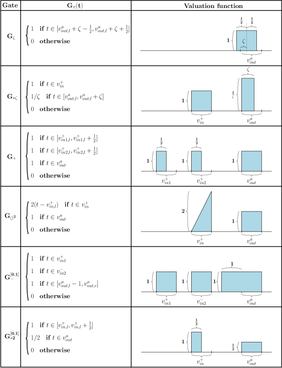
Figure 1: Gates and their corresponding functions $G_{\pi}(t)$.

The reduction follows the general outline of the reduction given in [28]. The construction is quite involved, and so we focus on the high-level picture here.

Each gate is implemented by 4 agents, namely $ad,mid,cen,ex$ in the Consensus Halving instance. The values computed by the gates are encoded by the positions of the cuts that are required in order to satisfy these agents. Agent $ad$ performs the exact mathematical operation of the gate, and feeds the outcome in $mid$, who “trims” it in accordance with the gate’s actual operation. Then $mid$ feeds her outcome to $cen$ and $ex$, who make a copy of $mid$’s correct value of the gate, with “negative” and “positive” labels respectively. This value with the appropriate label will be input to other gates.

The most important agents are the ones that perform the mathematical operation of each gate, i.e. agents $ad$. Figure 1 shows the part of the valuation functions of these agents that perform the operation. Each figure shows a valuation function for one of the agents, meaning that the blue regions represent portions of the object that the agent desires. The agent’s valuation for any particular interval is the integral of this function over that interval.

To understand the high-level picture of the construction, let us look at the construction for $G_{*\zeta}$. The precise valuation functions of the agents in the construction (see (2)) ensure that there is exactly one input cut in the region $v_{in}^{+}$. The leftmost piece due to that cut in that region will belong to $A_{+}$, while the rightmost will belong to $A_{-}$. It is also ensured that there is exactly one output cut in the region $v_{out}^{a}$, and that the first piece in that region will belong to $A_{-}$ and the second will belong to $A_{+}$.

Suppose that gate $g_{i}$ in the circuit is of type $G_{*\zeta}$ and we want to implement it through a Consensus Halving instance. If we treat $v_{in}^{+}$ and $v_{out}^{a}$ in Figure 1 as representing $[0,1]$, then agent $ad_{i}$ will take as input a cut at point $x\in v_{in}^{+}$. In order to be satisfied, $ad_{i}$ will impose a cut at point $y\in v_{out}^{a}$, such that $F_{i}(A_{+})=F_{i}(A_{-})$, where: $F_{i}(A_{+})=x+(\zeta-y)/\zeta$ and $F_{i}(A_{-})=(1-x)+y/\zeta$. Simple algebraic manipulation can be used to show that $ad_{i}$ is satisfied only when $y=\zeta\cdot x$, as required.

We show that the same property holds for each of the gates in Figure 1. Two notable constructions are for the gates $G_{()^{2}}$ and $G^{[0,1]}_{-}$. For the gate $G_{()^{2}}$ the valuation function of agent $ad$ is non-constant, which is needed to implement the non-linear squaring function. For the gate $G^{[0,1]}_{-}$, note that the output region $v_{out}^{a}$ only covers half of the possible output space. The idea is that if the result of $x[v_{in1}]-x[v_{in2}]$ is negative, then the output cut will lie before the output region, which will be interpreted as a zero output by agents $mid,cen,ex$ in the construction. On the other hand, if the result is positive, the result will lie in the usual output range, and will be interpreted as a positive number. An example where $x[v_{in1}]=1/4$ and $x[v_{in2}]=3/4$ is shown in Figure 2.

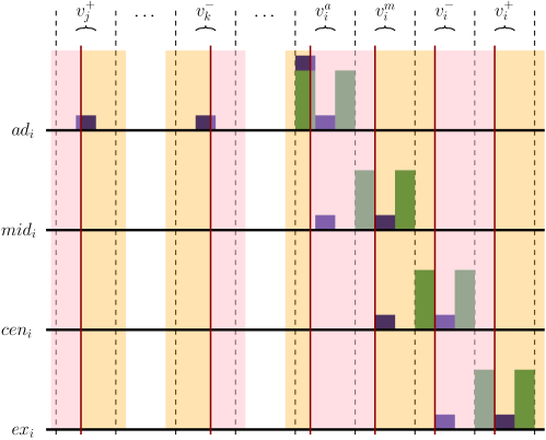
Figure 2: An example where the computation at the output $v_{out}:=v_{i}$ of a $G_{-}^{[0,1]}$ gate with inputs $v_{in1}:=v_{j}$ and $v_{in2}:=v_{k}$ is simulated by the Consensus Halving instance. Here $x[v_{j}]=1/4$ and $x[v_{k}]=3/4$, hence $x[v_{i}]=0$. The information about the values of the inputs is encoded by the cuts (red lines) in intervals $v_{j}^{+}$, and $v_{k}^{-}$ imposed by agents $ex_{j}$ and $cen_{k}$ respectively. The blue and green shapes depict the area below the valuation function of each of the 4 agents. The pink regions have label “$+$” while the yellow have label “$-$”. Agent $ad_{i}$ performs the subtraction, by demanding that she is satisfied, and places a cut $1/10$ to the left of the left endpoint of interval $v_{i}^{a}$. Then agent $mid_{i}$ gets satisfied by placing a cut at exactly the left endpoint of interval $v_{i}^{m}$, thus encoding the value 0 which is the correct output value of the gate. Finally, agents $cen_{i},ex_{i}$ copy this value by enforcing similar cuts at the left endpoints of intervals $v_{i}^{-}$ and $v_{i}^{+}$ respectively. The encoded values in the latter two intervals are the “negative” and “positive” version of $x[v_{i}]$.

Ultimately, this allows us to construct a Consensus Halving instance that implements this circuit. This means that for any $x\in[0,1]^{n}$, we can encode $x$ as a set of cuts, which then force cuts to be made at each gate gadget that encode the correct output for that gate.

Lemma 10.

Suppose that we are given an arithmetic circuit with the following properties.

• The circuit uses the gates $G_{\zeta},G_{+},G_{*\zeta},G_{()^{2}},G_{-}^{[0,1]},G_{*2}^{[0,1]}$.

• Every $G_{\zeta}$ and $G_{*\zeta}$ has $\zeta\in\mathbb{Q}\cap(0,1]$.

• For every input $x\in[0,1]^{n}$, all intermediate values computed by the circuit lie in $[0,1]$.

We can construct a Consensus Halving instance that implements this circuit.

The proof of this lemma is presented in Section 6.

5.2 $(n,n)$-Consensus Halving is $\mathtt{FIXP}$-hard

We show that $(n,n)$-Consensus Halving is $\mathtt{FIXP}$-hard by reducing from the problem of finding a Nash equilibrium in a $d$-player game, which is known to be $\mathtt{FIXP}$-complete [27]. As shown in [27], this problem can be reduced to the Brouwer fixed point problem: given an arithmetic circuit computing a function $F:[0,1]^{n}\to[0,1]^{n}$, find a point $x\in[0,1]^{n}$ such that $F(x)=x$. In a similar way to [28], we take this circuit and embed it into a Consensus Halving instance, with the outputs looped back to the inputs. Since Lemma 10 implies that our implementation of the circuit is correct, this means that any solution to the Consensus Halving problem must encode a point $x$ satisfying $F(x)=x$.

One difficulty is that we must ensure that the arithmetic circuit that we build falls into the class permitted by Lemma 10. To do this, we carefully analyse the circuits produced in [27], and we modify them so that all of the preconditions of Lemma 10 hold. This gives us the following result.

Theorem 11.

$(n,n)$-Consensus Halving is $\mathtt{FIXP}$-hard.

The proof of this theorem is presented in Section 7. Theorem 11, together with Theorem 6 give the following corollary.

Corollary 12.

$\mathtt{FIXP}$ $\subseteq$ $\mathtt{BU}$.

5.3 $(n,n-1)$-Consensus Halving is $\mathtt{ETR}$-complete

We will show the $\mathtt{ETR}$-hardness of $(n,n-1)$-Consensus Halving by reducing from the following problem $\textsc{Conjuction}_{[0,1]}$, which we prove it is $\mathtt{ETR}$-complete.

Definition 13 ($\textsc{Conjuction}_{[0,1]}$).

Let $p_{1},\ldots,p_{k}:[0,1]^{n}\to\mathbb{R}$ be a family of polynomials, where each one of them is given as a sum of monomials with integer coefficients. $\textsc{Conjuction}_{[0,1]}$ asks whether the polynomials have a common zero.

Then, we reduce the above problem to the following one.

Definition 14 (Feasible, $\textsc{Feasible}_{[0,1]}$).

Let $p(x_{1},\dots,x_{m})$ be a polynomial. Feasible asks whether there exists a point $(x_{1},\dots,x_{m})\in\mathbb{R}^{m}$ that satisfies $p(x_{1},\dots,x_{m})=0$. $\textsc{Feasible}_{[0,1]}$ asks whether there exists a point $(x_{1},\dots,x_{m})\in[0,1]^{m}$ that satisfies $p(x_{1},\dots,x_{m})=0$.

The idea is to turn the polynomial into a circuit, and then embed that circuit into a Consensus Halving instance using Lemma 10. As before, the main difficulty is ensuring that the preconditions of Lemma 10 are satisfied. To do this, we must ensure that the inputs to the circuit take values in $[0,1]$, which is not the case if we reduce directly from Feasible. Instead, we first consider the problem $\textsc{Feasible}_{[0,1]}$, in which $x$ is constrained to lie in $[0,1]^{n}$ rather than $\mathbb{R}^{n}$, and we show the following result.

Lemma 15.

$\textsc{Feasible}_{[0,1]}$ is $\mathtt{ETR}$-complete even for a polynomial of maximum sum of variable exponents in each monomial equal to 4.

The proof of that lemma is presented in Section 8. Consequently, via a polynomial-time reduction from $\textsc{Feasible}_{[0,1]}$ to $(n,n-1)$-Consensus Halving and Theorem 8, we prove the following result.

Theorem 16.

$(n,n-1)$-Consensus Halving is $\mathtt{ETR}$-complete.

The proof of the above theorem is presented in Section 9.

6 Proof of Lemma 10

In this section, the detailed construction of a Consensus Halving instance from an arbitrary given special circuit is presented. A special circuit is an arithmetic circuit with the properties described in the statement of Lemma 10 (see Section 5.1.1 for a detailed definition). After the construction, a correspondence of circuit to Consensus Halving solutions is proven, which completes the proof of the lemma.

6.1 Special circuit to Consensus Halving instance

Consider a circuit $H=(V,\mathcal{T})$ that uses gates in $\{G_{\zeta},G_{+},G_{*\zeta},G_{()^{2}},G_{-}^{[0,1]},G_{*2}^{[0,1]}\}$, with $\zeta\in\mathbb{Q}\cap(0,1]$, each gate’s inputs/output are in $[0,1]$, and both inputs of $G_{+}$ are in $[0,1/2]$. The constraints of the special gates $G_{()^{2}},G_{-}^{[0,1]},G_{*2}^{[0,1]}$ are shown in Table 2.

In general, the input of $H$ is a $N$-dimensional vector $x\in[0,1]^{N}$ is given by $N$ nodes with in-degree 0 and out-degree 1, called input-nodes. Also, in general, the output of $H$ is a $M$-dimensional vector $x^{\prime}\in[0,1]^{M}$ (the dimension of the circuit’s output is of no importance here). Moreover, it could be the case that $H$ is cyclic, meaning that it has no input and no output, but here we will consider the general case. Without loss of generality, let the rest of the nodes be of in-degree 1 and out-degree 1, located right after each gate’s output. By “right after” we mean that if a gate’s output has a branching, the node is placed before the branching. Suppose that the total number of nodes in $H$ is $r:=N+|\mathcal{T}|=poly(N)$, since by definition $H$ has polynomial size.

If the node $v_{i}\in V$ for $i\in[r]$ is at the output of gate $g_{i}$ we will call it the output-node of $g_{i}$ (otherwise it will be an input-node). For an example see Figure 3.

Figure 3: A node in series with the output of an addition gate. $v$ is the output-node of $g$.

Consider the node $v_{i}$, the output-node of gate $g_{i}$. $v_{i}$ corresponds to 4 Consensus Halving agents, named $ad_{i}$, $mid_{i}$, $cen_{i}$ and $ex_{i}$. Player $ad_{i}$ (Latin for “to”) represents the incoming edge to node $v_{i}$ and agent $ex_{i}$ (Latin for “from”) the outgoing edge from $v_{i}$, while both $mid_{i}$ and $cen_{i}$ represent an edge at the middle (center) of node $v_{i}$ that connects its input and output. The number of agents created in $H$ is $n:=4r$. The domain of the valuation functions of the agents is $[0,12r]$. Furthermore, this interval is split to $r$ blocks, with the $i$-th block being $[b_{i},b_{i+1}]$, where $b_{i}:=12(i-1)$, $i\in[r]$.

According to the definition of the Consensus Halving problem, the domain of the valuation functions of the agents is $[0,1]$. Although the domain of the valuation functions of the Consensus Halving instance that we reduce to is $[0,12r]$, this is just for convenience of presentation. In fact, by scaling down each block to length $1/(12r)$ (divide by $12r$), the domain becomes $[0,1]$ and the correctness of the reduction is preserved.

Let us define the function $border_{i}(t)$, $t\in[0,12r]$ for each node $v_{i}$, $i\in[r]$. The idea for this function is from [28]. If $v_{i}$ is the output-node of gate type $G_{*\zeta}$, then

$$border_{i}(t) =\begin{cases}4,\quad&t\in[b_{i},b_{i}+1]\cup[b_{i}+1+\zeta,b_{i}+2+\zeta]\\ 0,\quad&\text{otherwise}\end{cases}$$

If $v_{i}$ is the output-node of any gate type other than $G_{*\zeta}$, then

$$border_{i}(t) =\begin{cases}4,\quad&t\in[b_{i},b_{i}+1]\cup[b_{i}+2,b_{i}+3]\\ 0,\quad&\text{otherwise}\end{cases}$$

and also:

• $v_{i}^{a}:=[b_{i}+1,b_{i}+2]:=[v_{i,l}^{a},v_{i,r}^{a}]$

• $v_{i}^{m}:=[b_{i}+4,b_{i}+5]:=[v_{i,l}^{m},v_{i,r}^{m}]$

• $v_{i}^{-}:=[b_{i}+7,b_{i}+8]:=[v_{i,l}^{-},v_{i,r}^{-}]$

• $v_{i}^{+}:=[b_{i}+10,b_{i}+11]:=[v_{i,l}^{+},v_{i,r}^{+}]$

• $G_{\pi}(t)$ is the function corresponding to gate of type $G_{\pi}\in\{G_{\zeta},G_{*\zeta},G_{+},G_{()^{2}},G_{-}^{[0,1]},G_{*2}^{[0,1]}\}$ (see Figure 1).

The valuation functions of the agents $ad_{i}$, $mid_{i}$, $cen_{i}$ and $ex_{i}$ corresponding to node $v_{i}$ are,

$$ad_{i}(t) =\begin{cases}border_{i}(t)+G_{\pi}(t),\quad&\text{if $v_{i}$ is the output-node of gate type $G_{\pi}$}\\ border_{i}(t),\quad&\text{if $v_{i}$ is input-node (input of $H$)}.\end{cases}$$ (2)

$$mid_{i}(t) =\begin{cases}4,\quad&t\in[b_{i}+3,b_{i}+4]\cup[b_{i}+5,b_{i}+6]\\ 1,\quad&t\in v_{i}^{a}\cup v_{i}^{m}\\ 0,\quad&\text{otherwise}\end{cases}$$

$$cen_{i}(t) =\begin{cases}4,\quad&t\in[b_{i}+6,b_{i}+7]\cup[b_{i}+8,b_{i}+9]\\ 1,\quad&t\in v_{i}^{m}\cup v_{i}^{-}\\ 0,\quad&\text{otherwise}\end{cases}$$

$$ex_{i}(t) =\begin{cases}4,\quad&t\in[b_{i}+9,b_{i}+10]\cup[b_{i}+11,b_{i}+12]\\ 1,\quad&t\in v_{i}^{-}\cup v_{i}^{+}\\ 0,\quad&\text{otherwise}\end{cases}$$

The intuition for the synergy of the 4 agents is the following: Take as a given that in a solution of the created Consensus Halving instance with at most $n$ cuts, a cut is placed only (almost always) in the intervals $v_{i}^{a},v_{i}^{m},v_{i}^{-},v_{i}^{+}$ for every $i\in[r]$. Since the length of each of those intervals is 1, each such cut encodes a number in $[0,1]$. Consider $v_{i}$, the output-node of gate $g_{i}$ with inputs $v_{j},v_{k}$. Think of the agents $ad_{i}$, $mid_{i}$, $cen_{i}$, $ex_{i}$ as being sequential, meaning that each of them “computes” a value via a cut in $v_{i}^{a},v_{i}^{m},v_{i}^{-}$ or $v_{i}^{+}$ respectively, and feeds it in the next agent. In particular, agent $ad_{i}$ takes as input the values (in the form of cuts) that nodes $v_{j},v_{k}$ give her, and computes the exact operation that $g_{i}$ prescribes (e.g. if $g_{i}$ is type $G_{-}^{[0,1]}$, $ad_{i}$ performs subtraction of the input values without capping at 0, see Figure 2). Then $ad_{i}$ feeds this value in $mid_{i}$ via creating a cut in $v_{i}^{a}$, and $mid_{i}$ computes the actual value in $[0,1]$ that $g_{i}$ should output (e.g. if $g_{i}$ is type $G_{-}^{[0,1]}$, in this step $mid_{i}$ caps the value at 0), and feeds it in $cen_{i}$ via creating a cut in $v_{i}^{m}$. This correct value should be exported for further use from other gates to which $v_{i}$ is input, but depending on these gates, the positive or negative of that value might be needed (by “positive” and “negative” we mean the label, not the actual sign of the value). That is why a negative version of this value is produced by $cen_{i}$ and a positive by $ex_{i}$, via a cut in $v_{i}^{-}$ and $v_{i}^{+}$ respectively. A negative(resp. positive) value is one encoded by a cut that defines an interval at its left which is negative(resp positive). Moreover, for every input-node $v_{j}$ we arbitrarily consider $ad_{j}$ to encode a negative value, therefore, since (by the structure of the Consensus Halving instance) the labels of the values induced by the 4 agents are alternating, the agents $mid_{i}$, $cen_{i}$, $ex_{i}$ encode a positive, negative, and positive value, respectively.

6.2 One-to-two correspondence of circuit values to Consensus Halving cuts

Here we show that a solution of the special circuit maps to one pair of Consensus Halving solutions (since the solutions come by definition in pairs of opposite signs of pieces), and any pair of Consensus Halving solutions maps to exactly one solution of the special circuit.

Let us define the functions $z_{i}(x)$, $i\in[r]$ that depend on the input vector $x\in[0,1]^{N}$, and compute the value of each node $v_{i}$ of the arithmetic circuit $H$. Let us also, without loss of generality, set $(z_{1},\dots,z_{N}):=(x_{1},\dots,x_{N})$. First, we will show that for every tuple $(z_{1}(x),\dots,z_{r}(x))$ of values that satisfy $H$, a solution in the constructed Consensus Halving instance with $n$ agents and $n$ cuts ($n:=4r$) encodes the same values via its cuts. We will then show that for every solution of the Consensus Halving instance with $n$ agents and $n$ cuts, the cuts correspond to a unique tuple $(z_{1},\dots,z_{r})$ that satisfies $H$.

In the sequel, we call a cut $t$ negative(resp. positive) if the interval that it defines at its left has negative(resp. positive) label. Also, in the following subsections, the analysis is done for the case where the resulting Consensus Halving solution has its leftmost interval being negative. However, there is one more solution symmetric to this, in which the leftmost interval is positive. In any solution we remind that the intervals are of alternating signs (see definition of a Consensus Halving solution in Section 2.2). We omit the analysis of the solution where the leftmost interval is positive since it is identical to the presented one.

6.2.1 Circuit values to cuts

Suppose the tuple $(z_{1}^{*},\dots,z_{r}^{*})$ satisfies $H$. We will show that from this solution we can create a Consensus Halving solution with $n:=4r$ cuts, i.e. all of the agents are satisfied. Consider node $v_{i}$ of $H$. Let us translate the values $z_{i}^{*}$, $i\in[r]$ into cuts as follows:

• If $g_{i}$’s type is one of $G_{\zeta},G_{*\zeta},G_{+},G_{()^{2}},G_{*2}^{[0,1]}$ or $v_{i}$ is an input-node.

  • Place a cut at $t=v_{i,l}^{a}+z_{i}^{*}$,

  • Place a cut at $t=v_{i,l}^{m}+z_{i}^{*}$,

  • Place a cut at $t=v_{i,l}^{-}+z_{i}^{*}$,

  • Place a cut at $t=v_{i,l}^{+}+z_{i}^{*}$.

• If $g_{i}$’s type is $G_{-}^{[0,1]}$, i.e. $g_{i}=\max\{g_{j}-g_{k},0\}$, and $z_{j}^{*}\geq z_{k}^{*}$.

  • Place a cut at $t=v_{i,l}^{a}+z_{i}^{*}$,

  • Place a cut at $t=v_{i,l}^{m}+z_{i}^{*}$,

  • Place a cut at $t=v_{i,l}^{-}+z_{i}^{*}$,

  • Place a cut at $t=v_{i,l}^{+}+z_{i}^{*}$.

• If $g_{i}$’s type is $G_{-}^{[0,1]}$, i.e. $g_{i}=\max\{g_{j}-g_{k},0\}$, and $z_{j}^{*}<z_{k}^{*}$

  • Place a cut at $t=v_{i,l}^{a}-(z_{k}^{*}-z_{j}^{*})/5$,

  • Place a cut at $t=v_{i,l}^{m}+z_{i}^{*}$,

  • Place a cut at $t=v_{i,l}^{-}+z_{i}^{*}$,

  • Place a cut at $t=v_{i,l}^{+}+z_{i}^{*}$.

By construction of the valuation functions of the agents, these cuts are placed one after the other, where there is one cut in each of the intervals $v_{i}^{a}$, $v_{i}^{m}$, $v_{i}^{-}$, $v_{i}^{+}$ in that order, and each such sequence of four cuts is in an increasing order of $i$. By definition, any solution of Consensus Halving has alternating signs of the resulting pieces, and, as mentioned earlier, each solution comes with another symmetric solution with the same cuts and opposite signs of pieces. The analysis here is shown for the solution where the leftmost piece is negative, and we omit the analysis of the symmetric solution since it is identical.

Let us now prove that for every $i\in[r]$, the $ad_{i}$ agent is satisfied.

$\mathbf{G_{\zeta}:}$

This gate has no input. Consider its output $z_{i}^{*}=\zeta$ and its output-node $v_{i}$. By our constructed $n$-cut, a cut is placed at $t=v_{i,l}^{a}+\zeta$. Since the valuation function of $ad_{i}$ is symmetric around $v_{i,l}^{a}+\zeta$ (see aforementioned equation (2) that describes the valuation functions), the total valuation is cut exactly in half (see Figure 1), therefore agent $ad_{i}$ is satisfied.

$\mathbf{G_{*\zeta}:}$

Consider its input $z_{j}^{*}$, output $z_{i}^{*}=\zeta\cdot z_{j}^{*}$ and its output-node $v_{i}$. By our constructed $n$-cut, a positive cut is placed at $t=v_{j,l}^{+}+z_{j}^{*}$ and a negative cut is placed at $t=v_{i,l}^{a}+z_{i}^{*}$. Agent $ad_{i}$ is satisfied since her positive valuation equals her negative one. In particular, $z_{j}^{*}\cdot 1+(\zeta-z_{i}^{*})\cdot\frac{1}{\zeta}+1\cdot 4=(1-z_{j}^{*})\cdot 1+1\cdot 4+z_{i}^{*}\cdot\frac{1}{\zeta}$ is true.

$\mathbf{G_{+}:}$

Consider its inputs $z_{j}^{*}$, $z_{k}^{*}$, its output $z_{i}^{*}=z_{j}^{*}+z_{k}^{*}$ and its output-node $v_{i}$. By our constructed $n$-cut, a positive cut is placed at $t=v_{j,l}^{+}+z_{j}^{*}$, another positive cut is placed at $t=v_{k,l}^{+}+z_{k}^{*}$ and a negative cut is placed at $t=v_{i,l}^{a}+z_{i}^{*}$. Agent $ad_{i}$ is satisfied since her positive valuation equals her negative one. In particular, $z_{j}^{*}\cdot 1+z_{k}^{*}\cdot 1+(1-z_{i}^{*})\cdot 1+1\cdot 4=(1/2-z_{j}^{*})\cdot 1+(1/2-z_{k}^{*})\cdot 1+1\cdot 4+z_{i}^{*}\cdot 1$ is true.

$\mathbf{G_{()^{2}}:}$

Consider its input $z_{j}^{*}$, output $z_{i}^{*}=(z_{j}^{*})^{2}$ and its output-node $v_{i}$. By our constructed $n$-cut, a positive cut is placed at $t=v_{j,l}^{+}+z_{j}^{*}$ and a negative cut is placed at $t=v_{i,l}^{a}+z_{i}^{*}$. Agent $ad_{i}$ is satisfied since her positive valuation equals her negative one. In particular, $(z_{j}^{*})^{2}+(1-z_{i}^{*})\cdot 1+1\cdot 4=(1-(z_{j}^{*})^{2})+1\cdot 4+z_{i}^{*}\cdot 1$ is true.

$\mathbf{G_{*2}^{[0,1]}:}$

Consider its input $z_{j}^{*}$, output $z_{i}^{*}=2\cdot z_{j}^{*}$ and its output-node $v_{i}$. By our constructed $n$-cut, a positive cut is placed at $t=v_{j,l}^{+}+z_{j}^{*}$ and a negative cut is placed at $t=v_{i,l}^{a}+z_{i}^{*}$. Agent $ad_{i}$ is satisfied since her positive valuation equals her negative one. In particular, $z_{j}^{*}\cdot 1+(1-z_{i}^{*})\cdot\frac{1}{2}+1\cdot 4=(1/2-z_{j}^{*})\cdot 1+1\cdot 4+z_{i}^{*}\cdot\frac{1}{2}$ is true.

$\mathbf{G_{-}^{[0,1]}:}$

Consider its inputs $z_{j}^{*}$, $z_{k}^{*}$, its output $z_{i}^{*}=\max\{z_{j}^{*}-z_{k}^{*},0\}$ and its output-node $v_{i}$. By our constructed $n$-cut,

• if $z_{j}^{*}\geq z_{k}^{*}$, then $z_{i}^{*}=z_{j}^{*}-z_{k}^{*}$. By our constructed $n$-cut, a positive cut is placed at $t=v_{j,l}^{+}+z_{j}^{*}$, a negative cut is placed at $t=v_{k,l}^{-}+z_{k}^{*}$ and another negative cut is placed at $t=v_{i,l}^{a}+z_{i}^{*}$. Agent $ad_{i}$ is satisfied since her positive valuation equals her negative one. In particular, $z_{j}^{*}\cdot 1+(1-z_{k}^{*})\cdot 1+(1-z_{i}^{*})\cdot 1+1\cdot 4=(1-z_{j}^{*})\cdot 1+z_{k}^{*}\cdot 1+1\cdot(1+4)+z_{i}^{*}\cdot 1$ is true.

• if $z_{j}^{*}<z_{k}^{*}$, then $z_{i}^{*}=0$. By our constructed $n$-cut, a positive cut is placed at $t=v_{j,l}^{+}+z_{j}^{*}$, a negative cut is placed at $t=v_{k,l}^{-}+z_{k}^{*}$ and another negative cut is placed at $t=v_{i,l}^{a}-(z_{k}^{*}-z_{j}^{*})/5$. Agent $ad_{i}$ is satisfied since her positive valuation equals her negative one. In particular, $z_{j}^{*}\cdot 1+(1-z_{k}^{*})\cdot 1+\frac{z_{k}^{*}-z_{j}^{*}}{5}\cdot(1+4)+1\cdot 1+1\cdot 4=(1-z_{j}^{*})\cdot 1+z_{k}^{*}\cdot 1+(1-\frac{z_{k}^{*}-z_{j}^{*}}{5})\cdot(1+4)$ is true.

We will now prove that in our constructed $n$-cut, the agents $mid_{i}$, $cen_{i}$, $ex_{i}$ are also satisfied. If $g_{i}$ is not a $G_{-}^{[0,1]}$ gate, let us prove that $mid_{i}$ is satisfied. In our $n$-cut there is a negative cut at $t=v_{i,l}^{a}+z_{i}^{*}$ and a positive one at $t=v_{i,l}^{m}+z_{i}^{*}$. Agent $mid_{i}$ is satisfied since her negative valuation equals her positive one. In particular, $z_{i}^{*}\cdot 1+(1-z_{i}^{*})\cdot 1+1\cdot 4=(1-z_{i}^{*})\cdot 1+1\cdot 4+z_{i}^{*}\cdot 1$ is true.

If $g_{i}$ is a $G_{-}^{[0,1]}$ gate, let us prove that $mid_{i}$ is satisfied.

• if $z_{j}^{*}\geq z_{k}^{*}$, then a negative cut is placed at $t=v_{i,l}^{a}+z_{i}^{*}$, and a positive cut is placed at $t=v_{i,l}^{m}+z_{i}^{*}$. Agent $mid_{i}$ is satisfied since her negative valuation equals her positive one. In particular, $z_{i}^{*}\cdot 1+(1-z_{i}^{*})\cdot 1+1\cdot 4=(1-z_{i}^{*})\cdot 1+1\cdot 4+z_{i}^{*}\cdot 1$ is true.

• if $z_{j}^{*}<z_{k}^{*}$, then a negative cut is placed at $t=v_{i,l}^{a}-(z_{k}^{*}-z_{j}^{*})/5$ and a positive cut is placed at $t=v_{i,l}^{m}$. Agent $mid_{i}$ is satisfied since her negative valuation equals her positive one. In particular, $\frac{z_{k}^{*}-z_{j}^{*}}{5}\cdot 0+1\cdot 1+1\cdot 4=1\cdot 1+1\cdot 4+0\cdot 1$ is true.

For the agents $cen_{i}$ and $ex_{i}$, since their valuation functions are the same as $mid_{i}$ shifted to the right, it is easy to see that the $n$-cut we provide forces them to have positive valuation equal to their negative one.

6.2.2 Cuts to circuit values

Now suppose that the tuple $(t_{1}^{*},\dots,t_{n}^{*})$ with $0\leq t_{1}^{*}\leq\dots\leq t_{n}^{*}\leq 12r$, represents an $n$-cut ($n:=4r$) that is a solution of the constructed Consensus Halving instance with $n$ agents, where w.l.o.g. the first $4N$ cuts correspond to the $N$ input-nodes. We will show that from this solution we can construct a tuple $(z_{1},\dots,z_{r})$ that satisfies the circuit $H$. Again, note that solutions of Consensus Halving come in pairs, where the two solutions have the same cuts but opposite signs of pieces. We will only analyse the solution where the leftmost interval has negative sign and omit the symmetric case with positive leftmost interval since the analysis is identical and both Consensus Halving solutions map to the same circuit solution.

Consider node $v_{i}$ which is the output-node of gate $g_{i}$ or it is an input-node. Observe that the valuation function of each of $ad_{i},mid_{i},cen_{i}$ and $ex_{i}$ has more than half of her total valuation inside the interval $[b_{i},b_{i}+3],[b_{i}+3,b_{i}+6],[b_{i}+6,b_{i}+9]$ and $[b_{i}+9,b_{i}+12]$ respectively. This means that in a solution, each of them has to have at least one cut in her corresponding aforementioned interval. But since these intervals are not overlapping for all $n$ agents, and we need to have at most $n$ cuts, exactly one cut has to be placed by each agent in her corresponding interval.

Consider now the first $4N$ cuts that correspond to the input-nodes. As it is apparent from the definition of these nodes’ valuation functions, each agent of $ad_{i},mid_{i},cen_{i},ex_{i}$ for $i\in[N]$ has to place her single cut in the interval $v_{i}^{a},v_{i}^{m},v_{i}^{-},v_{i}^{+}$ respectively. Given the latter fact, the definition of valuation functions for non input-node agents dictates that there will always be a cut in $v_{i}^{+}$ for every $i\in[r]$. Since $0\leq t_{1}^{*}\leq\dots\leq t_{n}^{*}\leq 12r$, the sequential nature of our agents indicates that the cut $t_{4i}^{*}$, i.e. with index $4\cdot i$, is found in interval $v_{i}^{+}$. Now, let us translate the position of the cut $t_{4i}^{*},i\in[r]$ into the value $z_{i}=t_{4i}^{*}-v_{i,l}^{+}$. By a similar argument as that of the previous paragraph showing that the $ad_{i}$ agents are satisfied, it is easy to see that, by the aforementioned translation, the created tuple $(z_{1},\dots,z_{r})$ satisfies circuit $H$.

6.2.3 Valuation functions to circuits

In the Consensus Halving instances we construct, we have described the valuation functions of the agents mathematically. However, in a Consensus Halving instance the input is an arithmetic circuit, therefore we have to turn each valuation function of each agent $j\in[n]$ into its integral, and subsequently into an arithmetic circuit. Here we describe a method to do that.

The valuation functions we construct in our reduction (see Section 6.1) are piecewise polynomial functions of a single variable and their degree is at most 1, with $k$ pieces where $k$ is constant. Therefore, their integrals, which are the input of the Consensus Halving problem (captured by arithmetic circuits), are piecewise polynomial functions (with the same pieces) with degree at most 2. Consider the valuation function $f$ of an arbitrary player. Let the pieces of $f$ be $[p_{0},p_{1}),[p_{1},p_{2}),\dots,[p_{k-1},p_{k}]$ where $p_{0}=0$ and $p_{k}=1$ and denote $P_{1},P_{2},\dots,P_{k}$ the above pieces respectively. Let us also denote by $f^{P_{s}}$ the polynomial in interval $P_{s}$, $s\in\{1,2,\dots,k\}$. In particular, $f$ can be defined as

$$f(t)=\begin{cases}f^{P_{1}}(t)\quad,t\in[p_{0},p_{1})\\ f^{P_{2}}(t)\quad,t\in[p_{1},p_{2})\\ \vdots\\ f^{P_{k}}(t)\quad,t\in[p_{k-1},p_{k}],\end{cases}$$ (3)

and according to the valuation functions used in the reduction (see Section 6.1), for any given piece $P_{s}$ there are two kinds of possible functions

1. $f^{P_{s}}(t)=c_{s}$, where $c_{s}\geq 0$ is a constant, or

2. $f^{P_{s}}(t)=2\cdot(t-p_{s-1})$.

(The latter comes from the valuation function of an $ad$ agent that corresponds to an output node of a $G_{()^{2}}$ gate.)

We would like to find a formula for the integral of $f(t)$, denoted $F(t)$, and we also require that $F(t)$ is computable by an arithmetic circuit, so that it is a proper input (together with the other agents’ integrals of valuation functions) to the Consensus Halving instance. For each piece $P_{s}$ we will construct an integral, denoted by $F^{P_{s}}(t)$, such that each such integral will be computable by an arithmetic circuit, and so that it will be $F(t)=\sum_{s\in\{1,2,\dots,k\}}F^{P_{s}}(t)$. First, let us construct the function $D_{s}(t)$ using the domain $P_{s}$ of $f^{P_{s}}(t)$:

$$D_{s}(t):=\min\left\{\max\left\{t,p_{s-1}\right\},p_{s}\right\},$$

which takes values

$$D_{s}(t)=\begin{cases}p_{s-1},&t<p_{s-1}\\ t,&t\in[p_{s-1},p_{s}]\\ p_{s},&t>p_{s}.\end{cases}$$

Now, for function $f^{P_{s}}(t)$ of case (a), we construct its integral:

$$F^{P_{s}}(t):=c_{s}\cdot\left(D_{s}(t)-p_{s-1}\right),$$

which takes values

$$F^{P_{s}}(t)=\begin{cases}0,&t<p_{s-1}\\ c_{s}\cdot\left(t-p_{s-1}\right),&t\in[p_{s-1},p_{s}]\\ c_{s}\cdot\left(p_{s}-p_{s-1}\right),&t>p_{s}.\end{cases}$$

Similarly, for function $f^{P_{s}}(t)$ of case (b), we also construct its integral:

$$F^{P_{s}}(t):=\left(D_{s}(t)-p_{s-1}\right)^{2},$$

which takes values

$$F^{P_{s}}(t)=\begin{cases}0,&t<p_{s-1}\\ \left(t-p_{s-1}\right)^{2},&t\in[p_{s-1},p_{s}]\\ \left(p_{s}-p_{s-1}\right)^{2},&t>p_{s}.\end{cases}$$

Finally, for the agent with valuation function $f(t)$, the corresponding function computable by the arithmetic circuit that is input to the Consensus Halving problem is:

$$F(t):=\sum_{s\in\{1,2,\dots,k\}}F^{P_{s}}(t).$$

For the integral function $F(t)$ indeed it holds that $F(t)=\int_{0}^{t}f(x)\,dx$ as required. That is because, by the way we defined each $F^{P_{s}}(t)$, for any $t\in P_{s^{*}}$ it is

$$F(t)=\sum_{s\in\{1,2,\dots,k\}}F^{P_{s}}(t) =\sum_{s\in\{1,2,\dots,s^{*}-1\}}F^{P_{s}}(t)+F^{P_{s}^{*}}(t)+\sum_{s\in\{s^{*}+1,\dots,k\}}0$$

$$=\sum_{s\in\{1,2,\dots,s^{*}-1\}}\int_{P_{s}}f^{P_{s}}(x)\,dx+\int_{p_{s^{*}-1}}^{t}f^{P_{s}^{*}}(x)\,dx$$

$$=\sum_{s\in\{1,2,\dots,s^{*}-1\}}\int_{p_{s-1}}^{p_{s}}f(x)\,dx+\int_{p_{s^{*}-1}}^{t}f(x)\,dx$$

$$=\int_{0}^{t}f(x)\,dx$$

For each player with some valuation function $f$ as defined above, we can compute the functions $F^{P_{s}}$, $s\in[k]$ by using gates $G_{\zeta},G_{*\zeta},G_{-},G_{*},G_{min},G_{max}$. Then $F(t)$ can be computed by using $G_{+}$ gates. The arithmetic circuits that compute the functions $F(t)$ (one for each agent $j\in[n]$) constitute a proper Consensus Halving instance. This completes the proof of Lemma 10.

7 Proof of Theorem 11

In this section we give a detailed proof of Theorem 11 which states that $(n,n)$-Consensus Halving is $\mathtt{FIXP}$-hard. This is accomplished by finding a polynomial-time reduction from the $\mathtt{FIXP}$-complete problem of computing a “$d$-player Nash equilibrium” to the $(n,n)$-Consensus Halving problem. Using the machinery of [27], the $\mathtt{FIXP}$-complete problem is first expressed as a circuit with particular properties, which is then embedded into a $(n,n)$-Consensus Halving instance using Lemma 10. We prove that all of these steps can be executed in polynomial time.

In particular, in [27] it is shown that the problem of finding a Nash equilibrium of a $d$-player normal form game with $d\geq 3$ (“$d$-player Nash equilibrium” problem) is $\mathtt{FIXP}$-complete. Given an instance of this problem, we will construct a polynomial-time reduction to $(n,n)$-Consensus Halving. We will start from an arbitrary instance of “$d$-player Nash equilibrium” and, according to it, design a circuit using only the gates $G_{\zeta},G_{+},G_{-},G_{*},G_{\max},G_{\min}$ with $\zeta\in\mathbb{Q}$. This step is done by a straightforward application of the procedure described in the proofs of Lemma 4.5 and Lemma 4.6 in [27]. This circuit computes a function whose fixed points correspond precisely to the Nash equilibria of the initial game. Then, we create an equivalent circuit by “breaking down” the initial gates to some more suitable ones (by introducing “special gates”, see Table 2), whose inputs and outputs are guaranteed to be in $[0,1]$. From this, we will create a cyclic circuit, introduce Consensus Halving players on the “wires” of the circuit, and show that a Consensus Halving solution with at most as many cuts as the number of players in this instance can be efficiently translated back to a Nash equilibrium of the initial game.

7.1 Expressing the game as a circuit without division gates

Here, given an arbitrary $d$-player game, we will employ a function presented in [27] whose fixed points are precisely the Nash equilibria of that game. Consider a given instance $I$ of the “$d$-player Nash equilibrium” problem, i.e. a $d$-player normal form game where each player $i$ has a set $S_{i}$ of pure strategies. We will use the following notation similar to the one in [27]: $N_{i}:=|S_{i}|$, $N:=\sum_{i}^{d}N_{i}$ and $v_{i}$ is the payoff function of player $i$ with domain $D_{I}:=\times_{i=1}^{d}\Delta_{N_{i}}$, where $\Delta_{N_{i}}$ is the unit $(N_{i}-1)$-simplex. Define the mixed strategy profile $x:=(x_{11},\dots,x_{1N_{1}},x_{21},\dots,x_{2N_{2}},\dots,x_{d1},\dots,x_{dN_{d}})$ to be a $N$-dimensional vector with the entry $x_{ij}$ being the probability that player $i\in[d]$ plays pure strategy $j\in S_{i}$. Also, $v(x)$ is an $N$-dimensional vector with entries indexed as in $x$, with $v_{ij}(x):=v_{i}(j,x_{-i})$, the latter being the expected payoff of player $i$ when she plays the pure strategy $j\in S_{i}$ against the partial profile $x_{-i}$ of the rest of the players. The payoff function of each player is normalized by scaling in $[0,1/N]$ so that the Nash equilibria of the game are precisely the same. Thus, $v_{ij}(x)\in[0,1/N]$. Finally, let $h(x):=x+v(x)$.

Now, define for each player $i$ the function $f_{i,x}(t):=\sum_{j\in S_{i}}\max(h_{ij}(x)-t,0)$ with parameter $x$. This function is defined in $\mathbb{R}$ and it is continuous, piecewise linear, strictly decreasing with values from $0$ to $+\infty$, thus there is a unique value $t_{i}\in\mathbb{R}$ such that $f_{i,x}(t_{i})=1$. The required function whose set of fixed points is identical to the set of Nash equilibria of instance $I$ is $G_{I}(x)_{ij}:=\max(h_{ij}(x)-t_{i},0)$ for $i\in[d]$, $j\in S_{i}$. The function $G_{I}$ takes as input the $n$-dimensional vector $x$ and outputs an $N$-dimensional vector $G_{I}(x)$ with entries defined as above. By definition of $G_{I}$ and choice of $t_{i}$, it is $\sum_{j\in S_{i}}G_{I}(x)_{ij}=1$ for every $i\in[d]$, and therefore $G_{I}$ is a mapping of the domain $D_{I}$ to itself.

Lemma 17 (LEMMA 4.5, [27]).

The fixed points of the function $G_{I}$ are precisely the Nash equilibria of the game $I$.

In fact, the structure of function $G_{I}$ allows for it to be efficiently constructed using only the required types of gates.

Lemma 18 (LEMMA 4.6, [27]).

We can construct in polynomial time a circuit with basis $\{+,-,*,\max,\min\}$ (no division) and rational constants that computes the function $G_{I}$.

For the proofs of the above lemmata the reader is referred to the indicated work by Etessami and Yannakakis.

In the proof of the latter lemma in [27] it is shown how to construct an arithmetic circuit $C_{I}$ that computes the function $G_{I}$ using only gates of type $G_{\zeta},G_{+},G_{-},G_{*},G_{\max},G_{\min}$, where $\zeta\in\mathbb{Q}$. The construction of $C_{I}$ is the following: Compute the function $y=h(x)=x+v(x)$ using only $G_{+},G_{*}$ type of gates, allowed by the definition of $v(x)$. Vector $y$ has $d$ sub-vectors, where $y_{i}=(y_{i1},y_{i2},\dots,y_{iN_{i}})$. Then, each $y_{i}$ is sorted using a sorting network $Z_{i}$ thus creating a vector $z_{i}=(z_{i1},z_{i2},\dots,z_{iN_{i}})$ with sorted entries $z_{i1}\geq z_{i2}\geq\dots\geq z_{iN_{i}}$; sorting networks can be implemented in arithmetic circuits using only gates $G_{\max},G_{\min}$ (for more see e.g. [35]). Using $z_{ij}$’s the function $t_{i}:=\max_{l\in[N_{i}]}\left\{(1/l)*\left(\left(\sum_{j=1}^{l}z_{ij}\right)-1\right)\right\}$ is computed and the final output of the whole circuit is

$$x_{ij}^{\prime}:=\max\{y_{ij}-t_{i},0\}\quad\text{ for each }i\in[d],j\in S_{i}.$$ (4)

7.2 A circuit with gates whose inputs/outputs are in $[0,1]$

One can easily observe that some of the gates of circuit $C_{I}$ may have inputs and outputs outside of $[0,1]$. For example, the $G_{+}$ gate that computes $y_{ij}=x_{ij}+v(x)_{ij}$ can be 2 and the arguments of $G_{\max}$ in $t_{i}$ can be negative. We will transform this circuit into an equivalent one that guarantees its gates’ inputs and outputs to be in $[0,1]$, using only gates $G_{\zeta},G_{+},G_{-}^{[0,1]},G_{*},G_{*2}^{[0,1]},G_{\max},G_{\min}$, where $\zeta\in\mathbb{Q}\cap(0,1]$.

In particular, instead of constructing the circuit $C_{I}$ as described in the previous paragraph, we will construct an equivalent one, called $C_{I}^{\prime}$, whose input and output are the same as that of $C_{I}$, namely $x_{ij}$ and $x_{ij}^{\prime}$, $i\in[d]$, $j\in[N_{i}]$ respectively, but its gates have inputs/outputs in $[0,1]$. We do this by manipulating the formula for the required function $G_{I}$ under computation, by suitably scaling up or down the input values of each gate, using additional gates $G_{\zeta},G_{+},G_{-}^{[0,1]},G_{*}$.

We construct $C_{I}^{\prime}$ as follows: First, we compute the vector $p:=h(x)/2=x*\frac{1}{2}+v(x)*\frac{1}{2}$ using only $G_{+},G_{*}$ gates. Note that $x_{ij},v_{ij}(x),p_{ij}\in[0,1]$, $\forall i\in[d],j\in S_{i}$ (recall that the payoff function is normalized in $[0,1]$). Then, we sort each of the sub-vectors $p_{i}$, $i\in[d]$ via a sorting network $Q_{i}$ that can be constructed using $G_{\max}$ and $G_{\min}$ gates, thus computing the sorted vectors $q_{i}=(q_{i1},q_{i2},\dots,q_{iN_{i}})$ with sorted entries $q_{i1}\geq q_{i2}\geq\dots\geq q_{iN_{i}}$. Now, for every $i\in[d]$ and $l\in[N_{i}]$ we compute the following sub-function

$$t_{il}^{\prime\prime}:=\frac{1}{2}*\frac{1}{l}*\sum_{j=1}^{l}q_{ij}+\frac{1}{2}-\frac{1}{4}*\frac{1}{l},$$

by using $l+1$ $G_{+}$ gates, 3 $G_{+}$ gates and 1 $G_{-}^{[0,1]}$ gate, where the subtraction gate is the last to take place. One should observe that since $\sum_{j=1}^{N_{i}}x_{ij}=1$ and $\sum_{j=1}^{N_{i}}v_{ij}(x)\leq 1$ (by definition of payoff function in $[0,1/N]$), it is $\sum_{j=1}^{N_{i}}q_{ij}\leq\frac{1}{2}\cdot\left(1+1\right)=1$, therefore none of the individual computations of $t_{il}^{\prime\prime}$ is outside $[0,1]$. Moreover, in the subtraction, the value of the subtrahend is at most the value of the minuend so the subtraction is precise (not capped at 0).

Now, for each $i\in[d]$ we compute the sub-function

$$t_{i}^{\prime\prime}:=\max_{l\in[N_{i}]}\{t_{il}^{\prime\prime}\},$$

by using $N_{i}-1$ $G_{\max}$ gates, and consequently compute

$$t_{i}^{\prime}:=\left(t_{i}^{\prime\prime}-\frac{1}{2}\right)*2,$$

by using one $G_{-}^{[0,1]}$ and one special $G_{*2}^{[0,1]}$ gate where the computations happen from left to right. Note that $t_{i}^{\prime\prime}\geq 1/2$, therefore the subtraction is precise (not capped at 0). Also, note that, by definition of $t_{il}^{\prime\prime}$, it is $t_{i}^{\prime\prime}\leq 1$, therefore $t_{i}^{\prime\prime}-1/2\leq 1/2$ and the output of the $G_{*2}^{[0,1]}$ gate of $t_{i}^{\prime}$ is in $[0,1]$. Finally, the output of the circuit $C_{I}^{\prime}$ is computed by

$$x_{ij}^{\prime}:=\max\{p_{ij}-t_{i}^{\prime},0\}*2,\quad\text{ for each }i\in[d],j\in S_{i},$$ (5)

using one $G_{-}^{[0,1]}$ and one special $G_{*2}^{[0,1]}$ gate.

Lemma 19.

Circuit $C_{I}^{\prime}$ is equivalent to $C_{I}$, i.e. it computes the function $G_{I}$.

Proof.

We will show that for every $i\in[d],j\in S_{i}$, the value $x_{ij}$ of (5) is the same as that of (4), i.e. the output of the circuits $C_{I}^{\prime}$ and $C_{I}$ is the exact same. Using the formulas for $t_{il}^{\prime\prime},t_{i}^{\prime\prime}$ and $t_{i}^{\prime}$, we can re-write algebraically $x_{ij}$ by substituting the circuit’s operations with the regular mathematical ones, i.e. $G_{+},G_{-}^{[0,1]},G_{*2}^{[0,1]},G_{*},G_{\max},G_{\min}$ translate to $+,-,\cdot 2,\cdot,\max,\min$ respectively. Observe that this is possible since the $G_{-}^{[0,1]}$ gate, excluding the one in (5), actually performs subtraction without capping the output to 0. Thus, starting from (5) we have

$$x_{ij}^{\prime} =\max\{p_{ij}-t_{i}^{\prime},0\}\cdot 2$$

$$=\max\{2\cdot p_{ij}-2\cdot t_{i}^{\prime},0\}$$

$$=\max\left\{y_{ij}-4\cdot\left(t_{i}^{\prime\prime}-\frac{1}{2}\right),0\right\}\quad\text{($y_{ij}$ from construction of $C_{I}$)}$$

$$=\max\left\{y_{ij}-4\cdot\left(\max_{l\in[N_{i}]}\{t_{il}^{\prime\prime}\}-\frac{1}{2}\right),0\right\}$$

$$=\max\left\{y_{ij}-4\cdot\left(\max_{l\in[N_{i}]}\left\{\frac{1}{2l}\cdot\left(\sum_{j=1}^{l}q_{ij}\right)+\frac{1}{2}-\frac{1}{4l}\right\}-\frac{1}{2}\right),0\right\}$$

$$=\max\left\{y_{ij}-4\cdot\max_{l\in[N_{i}]}\left\{\frac{1}{2l}\cdot\left(\sum_{j=1}^{l}q_{ij}\right)-\frac{1}{4l}\right\},0\right\}$$

$$=\max\left\{y_{ij}-\max_{l\in[N_{i}]}\left\{\frac{1}{l}\cdot\left(\sum_{j=1}^{l}2\cdot q_{ij}\right)-\frac{1}{l}\right\},0\right\}$$

$$=\max\left\{y_{ij}-\max_{l\in[N_{i}]}\left\{\frac{1}{l}\cdot\left(\left(\sum_{j=1}^{l}z_{ij}\right)-1\right)\right\},0\right\}\quad\text{($z_{ij}$ from construction of $C_{I}$)}$$

$$=\max\left\{y_{ij}-t_{i},0\right\}\quad\text{($t_{i}$ from construction of $C_{I}$)},$$

which is by definition equal to the output $x_{ij}^{\prime}$ of (4). ∎

The circuit $C_{I}^{\prime}$ we constructed that computes the function $G_{I}$ uses gates of type in the set $\{G_{\zeta},G_{+},G_{*},G_{\max},G_{\min},G_{-}^{[0,1]},G_{*2}^{[0,1]}\}$, where $\zeta\in\mathbb{Q}\cap(0,1]$.

7.3 The $(n,n)$-Consensus Halving instance

At this point we are ready to construct the $(n,n)$-Consensus Halving instance. The final circuit $C_{I}^{\prime}$ computes the function $G_{I}$, where $G_{I}:D_{I}\to D_{I}$, whose fixed points are precisely the Nash equilibria of the initial instance $I$ of the $d$-player game, due to Lemma 17. The output of $C_{I}^{\prime}$ is the $N$-dimensional vector $x^{\prime}$ with entries $x_{ij}^{\prime}$ computed from (5). Let us close the circuit by connecting the output $x_{ij}^{\prime}$ with the input $x_{ij}$ for every $i\in[d]$, $j\in S_{i}$. This new circuit, called $C_{I}^{o}$, is cyclic, meaning that it has no input and no output.

The cyclic circuit $C_{I}^{o}$ (like $C_{I}^{\prime}$) uses only gates in $\{G_{\zeta},G_{+},G_{*},G_{\max},G_{\min},G_{-}^{[0,1]},G_{*2}^{[0,1]}\}$, where $\zeta\in\mathbb{Q}\cap(0,1]$. In Section 5.1 we describe how to turn such circuits into Consensus Halving instances. Suppose that $C_{I}^{o}$ uses $l$ gates. Then, by the procedure of Section 5.1 let us turn $C_{I}^{o}$ into a special circuit $C_{I}^{o^{\prime}}$ with $r=linear(l)$ gates which uses only the required gates by Lemma 10. Finally, still following that procedure, let us turn $C_{I}^{o^{\prime}}$ into a Consensus Halving instance with $n:=4r$ agents.

We can now prove Theorem 11.

Proof.

In Section 6 it was proven that a solution to the above $(n,n)$-Consensus Halving instance, i.e. a solution with $n$ cuts, in linear time can be translated back to a tuple $z^{*}:=(z_{1}^{*},z_{2}^{*},\dots,z_{r}^{*})$ of satisfying values for the nodes of $C_{I}^{o^{\prime}}$. Recall that $C_{I}^{o^{\prime}}$ was created by another cyclic equivalent circuit $C_{I}^{o}$ which was also created by merging the input and output nodes of an acyclic circuit $C_{I}^{\prime}$.

Let us denote by $v_{1},v_{2},\dots,v_{N}$ and $v^{\prime}_{1},v^{\prime}_{2},\dots,v^{\prime}_{N}$ the input and output nodes respectively of $C_{I}^{\prime}$ and denote by $V_{1},V_{2},\dots,V_{N}$ the merged nodes in $C_{I}^{o}$ and $C_{I}^{o^{\prime}}$. Let us denote by $x^{*}:=(x_{1}^{*},x_{2}^{*},\dots,x_{N}^{*})$ the $N$ entries of $z^{*}$ that correspond to the values of nodes $(V_{1},V_{2},\dots,V_{N})$. Since the procedure in Section 5.1 which turns $C_{I}^{o}$ into $C_{I}^{o^{\prime}}$ preserves the computation of the values of $V_{1},V_{2},\dots,V_{N}$, it follows that $x^{*}$ satisfies $C_{I}^{o}$. Consequently, if the values $x^{*}$ are copied as values of both input $(v_{1},v_{2},\dots,v_{N})$ and output $(v^{\prime}_{1},v^{\prime}_{2},\dots,v^{\prime}_{N})$ nodes of $C_{I}^{\prime}$ then $C_{I}^{\prime}$ is satisfied, since these nodes of $C_{I}^{\prime}$ compute the same values as those that $V_{1},V_{2},\dots,V_{N}$ compute in $C_{I}^{o}$.

As it was shown in Lemma 19, the output of $C_{I}^{\prime}$ computes the same output as $C_{I}$, which computes the function $G_{I}$. Thus, for $x^{*}$ it holds that $G_{I}(x^{*})=x^{*}$, i.e. it is a fixed point of $G_{I}$. Recall now that the fixed points of $G_{I}$ are precisely the Nash equilibria of instance $I$ of the initial “$d$-player Nash equilibrium” problem. Since, due to [27], “$d$-player Nash equilibrium” is $\mathtt{FIXP}$-complete, it follows that $(n,n)$-Consensus Halving is $\mathtt{FIXP}$-hard. ∎

8 Proof of Lemma 15

Let us define the constrained version of $\mathtt{ETR}$, denoted $\mathtt{ETR}_{[0,1]}$, where the polynomials are over $[0,1]^{n}$. It is easy to see that $\mathtt{ETR}_{[0,1]}\subseteq\mathtt{ETR}$; an arbitrary $\mathtt{ETR}_{[0,1]}$ instance $\exists(X_{1},\dots,X_{m})\in[0,1]^{m}\cdot\Phi$, where $\Phi$ is the $\mathtt{ETR}_{[0,1]}$ formula, can be written as the following $\mathtt{ETR}$ instance $\exists(X_{1},\dots,X_{m})\in\mathbb{R}^{m}\cdot\Phi\bigwedge_{i=1}^{m}\left(\left(X_{i}\geq 0\right)\wedge\left(X_{i}\leq 1\right)\right)$.

Lemma 3.9 of [42] proves that the problem of deciding whether a family of polynomials $p_{i}:\mathbb{R}^{n}\to\mathbb{R}$, $i\in[k]$ has a common root in the $n$-dimensional unit-ball (with center $0^{n}$ and radius 1) is $\mathtt{ETR}$-complete. Furthermore, this holds even when all $p_{i}$’s have maximum sum of variable exponents in each monomial equal to 2. Since the $n$-dimensional unit-ball is inscribed in the $n$-dimensional unit-cube, the aforementioned result implies that $\textsc{Conjuction}_{[0,1]}$ is $\mathtt{ETR}$-hard, therefore $\mathtt{ETR}\subseteq\mathtt{ETR}_{[0,1]}$. Consequently, we get the following.

Theorem 20.

$\mathtt{ETR}_{[0,1]}=\mathtt{ETR}$.

Now we will prove that $\textsc{Feasible}_{[0,1]}$ is $\mathtt{ETR}$-hard by reducing $\textsc{Conjuction}_{[0,1]}$ to it. We do this by a standard way of turning a conjunction of polynomials into a single polynomial, so that all zeros of the conjunction are exactly the same as the zeros of the single polynomial. Consider an instance of $\textsc{Conjuction}_{[0,1]}$. Let us define the function $q=(p_{1})^{2}+(p_{2})^{2}+\dots+(p_{k})^{2}$, which has again domain $[0,1]^{n}$. The instance of $\textsc{Feasible}_{[0,1]}$ with function $q$ has exactly the same solutions as these of the $\textsc{Conjuction}_{[0,1]}$ instance. Therefore $\textsc{Feasible}_{[0,1]}$ is $\mathtt{ETR}$-complete, even when $q$ has maximum sum of variable exponents in each monomial equal to 4.

9 Proof of Theorem 16

As we show in Theorem 8, $(n,k)$-Consensus Halving is in $\mathtt{ETR}$. In this section we prove that $(n,n-1)$-Consensus Halving is $\mathtt{ETR}$-hard, implying that it is complete for $\mathtt{ETR}$. This complements the results of [28], where it was established that $(n,n-1)$-Consensus Halving is $\mathtt{NP}$-hard even when a solution is required to be $1/poly(n)$-approximately correct, i.e. it allows $|F_{i}(A_{+})-F_{i}(A_{-})|\leq\epsilon$ for every agent $i$, where $\epsilon=1/poly(n)$.

We present a polynomial-time reduction from the $\mathtt{ETR}$-complete problem $\textsc{Feasible}_{[0,1]}$ to $(n,n-1)$-Consensus Halving. Suppose we are asked to decide an arbitrary instance of $\textsc{Feasible}_{[0,1]}$, i.e. the existential sentence

$$\left(\exists X\in[0,1]^{N}\right)(p(X)=0),$$ (6)

where $X:=(X_{1},\dots,X_{N})\in[0,1]^{N}$ and $p$, is a polynomial function of $X_{1},\dots,X_{N}$ written in the standard form (a sum of monomials with integer coefficients). Consider the integer coefficients $C_{1},\dots,C_{l}$ of $p$, where the number of terms of the polynomial is $l$. We consider all of the coefficients to be positive, where some of them may be preceded by a “$+$” or a “$-$”. Also, let us normalize the coefficients and create new ones $c_{1},\dots,c_{l}$, where

$$c_{j}:=\frac{C_{j}}{l\cdot C_{max}},\quad j\in[l],$$

where $C_{max}:=\max_{j}C_{j}$. Note that our new polynomial $q(X)$ which uses the new coefficients has exactly the same roots as $p(X)$. Also, note that $c_{j}\in(0,\frac{1}{l}]$ for every $j\in[l]$, a fact that will play an important role at the last steps of our reduction.

Now, let us split polynomial $q$ into two polynomials $q_{1}$ and $q_{2}$, such that

$$q(X):=q_{1}(X)-q_{2}(X),$$

and both $q_{1}$ and $q_{2}$ are sums of positive terms; $l_{1}$ and $l_{2}$ terms of $q_{1}$ and $q_{2}$ respectively, where $l=l_{1}+l_{2}$. In particular,

$$q_{1}(X) :=\sum_{j=1}^{l_{1}}r_{j}(X),$$

$$q_{2}(X) :=\sum_{j=l_{1}+1}^{l_{2}}r_{j}(X),$$

where $r_{j}(X):=c_{j}\cdot X_{1}^{d_{1j}}\cdot\dots\cdot X_{N}^{d_{Nj}}$ is the term $j\in[l]$ and $d_{ij}$ is the exponent of variable $X_{i}$, $i\in[N]$, in the $j$-th term. Eventually, the existential sentence, equivalent to (6), that we ask to decide is

$$\left(\exists X\in[0,1]^{N}\right)(q_{1}(X)=q_{2}(X)).$$

Let us construct the algebraic circuit that takes as input the tuple $X$ and computes the value of $q_{1}(X)$. This circuit needs only to use gates in $\{G_{\zeta},G_{+},G_{*\zeta},G_{*},G_{()^{2}}\}$, where $\zeta\in\mathbb{Q}\cap(0,1]$. To see why, observe that since every $X_{i}\in[0,1]$, $i\in[N]$, any multiplication between them by a $G_{*}$ gate is done properly (the gate’s inputs/output are in $[0,1]$), and obviously the same holds for $G_{()^{2}}$. Also, note that due to our downscaled coefficients $c_{j}$, it is $c_{j}\leq 1/2$ for every $j$, and also

$$\sum_{j=1}^{l_{1}}r_{j}(X)\leq l_{1}/l\leq 1.$$ (7)

Therefore, we guarantee that any of the $l_{1}-1$ additions of the terms $r_{j}$ of $q_{1}$ by a $G_{+}$ gate is done properly, (inputs in $[0,1/2]$ and output in $[0,1]$). Similarly, we construct a circuit that computes $q_{2}$.

At this point we are ready to prove Theorem 16.

Proof.

Let us construct a $(n,n-1)$-Consensus Halving instance, where $n$ is to be defined later. In Section 5.1 we have shown how to construct an equivalent circuit to the one that computes $q_{1},q_{2}$, called “special circuit”, that

• uses only gates $G_{\zeta},G_{+},G_{*\zeta},G_{()^{2}},G_{-}^{[0,1]},G_{*2}^{[0,1]}$,

• every $G_{\zeta}$ and $G_{*\zeta}$ has $\zeta\in\mathbb{Q}\cap(0,1]$,

• for every input $x\in[0,1]^{N}$, all intermediate values computed by the circuit lie in $[0,1]$.

For the constraints of the above types of gates, see Tables 1, 2.

Let the number of gates in that special circuit be $r:=poly(N)$. Consider the last two nodes of the special circuit whose outgoing edges are $q_{1}$ and $q_{2}$ respectively. Without loss of generality, we name them $v_{r-1}$ and $v_{r}$ (see Figure 4).

Figure 4: The last two nodes of the special circuit.

By Lemma 10 and the construction described in its proof (Section 6), we embed the special circuit in a Consensus Halving instance. This instance now consists of $4r$ agents, since to each node $i\in[r]$ correspond 4 agents: $ad_{i},mid_{i},cen_{i}$ and $ex_{i}$ with valuation functions described by (2).

According to the embedding described in Section 6, a tuple $(z_{1}^{*},\dots,z_{r}^{*})$ of values that satisfies the special circuit, corresponds to a $(4r,4r)$-Consensus Halving solution, i.e. a tuple $(t_{1}^{*},\dots,t_{4r}^{*})$ with $0\leq t_{1}^{*}\leq\dots\leq t_{4r}^{*}\leq 12r$, of the Consensus Halving instance we constructed, and vice versa. As shown in detail in Section 6, every value $z_{i}^{*}$ in a solution can be translated to 4 cuts $t_{4i-3}^{*},t_{4i-2}^{*},t_{4i-1}^{*},t_{4i}^{*}$ in the Consensus Halving solution by the transformation in Section 6.2.1. Conversely, a 4-tuple $(t_{4i-3}^{*},t_{4i-2}^{*},t_{4i-1}^{*},t_{4i}^{*})$ of cuts in a Consensus Halving solution can be translated to a single value $z_{i}^{*}$ by the simple transformation $z_{i}^{*}=t_{4i}^{*}-v_{i,l}^{+}$ in Section 6.2.2.

Let us now introduce a $(4r+1)$-st additional agent, named finis (from the Latin word for “end”) who does not correspond to any node. The valuation function of this agent is non-zero only in the intervals $v_{r-1}^{+}$ and $v_{r}^{-}$ and, in particular is the following,

$$finis(t) =\begin{cases}1,\quad&t\in v_{r-1}^{+}\cup v_{r}^{-}\\ 0,\quad&\text{otherwise}.\end{cases}$$ (8)

Eventually, the number of agents in the embedding is $n:=4r+1$.

We will show that the answer to the arbitrary $\textsc{Feasible}_{[0,1]}$ instance (6) is “yes”, if and only if the answer to the $(n,n-1)-\textsc{Consensus Halving}$ problem is “yes”, i.e. there exists a $(n-1)$-cut that satisfies $n$ agents.

Suppose that there exists a solution $X^{*}:=(X_{1}^{*},\dots,X_{N}^{*})\in[0,1]^{N}$ of (6), which equivalently means that $q_{1}(X^{*})=q_{2}(X^{*})$. Then, by the correct construction of our special circuit (following the procedure in Section 5.1) which uses $r$ gates and computes $q_{1}$ and $q_{2}$, there is a tuple $z^{*}:=(z_{1}^{*},\dots,z_{r}^{*})$ that satisfies it. Let, without loss of generality, $(z_{1}^{*},\dots,z_{N}^{*}):=(X_{1}^{*},\dots,X_{N}^{*})$. Then it holds that $q_{1}(z_{1}^{*},\dots,z_{N}^{*})=q_{2}(z_{1}^{*},\dots,z_{N}^{*})$, therefore $z_{r-1}^{*}=z_{r}^{*}$.

According to the aforementioned translation to cuts, in the Consensus Halving instance there will be a cut $t_{4(r-1)}^{*}=v_{r-1,l}^{+}+z_{r-1}^{*}$ in interval $v_{r-1}^{+}$ (i.e. a positive cut), and another one in $t_{4r-1}^{*}=v_{r,l}^{-}+z_{r}^{*}$ in interval $v_{r}^{-}$ (i.e. a negative cut). From the valuation function (8) of agent $finis$, we can see that her positive total valuation equals her negative total valuation, since $z_{r-1}^{*}\cdot 1+(1-z_{r}^{*})\cdot 1=(1-z_{r-1}^{*})\cdot 1+z_{r}^{*}\cdot 1$ holds from $z_{r-1}^{*}=z_{r}^{*}$. Therefore $finis$ is satisfied. Also, the agents $ad_{i},mid_{i},cen_{i},ex_{i}$ for all $i\in[r]$ are satisfied as argued in Section 6, and the answer to $(n,n-1)-\textsc{Consensus Halving}$ is “yes”, since we have $4r+1$ agents satisfied by $4r$ cuts.

Suppose now that there exists a $4r$-cut $(t_{1}^{*},\dots,t_{4r}^{*})$ with $0\leq t_{1}^{*}\leq\dots\leq t_{4r}^{*}\leq 12r$ that is a solution of the $(n,n-1)$-Consensus Halving instance we constructed, where $n:=4r+1$. As argued in Section 6, if the $ad_{i},mid_{i},cen_{i},ex_{i}$ agents for $i\in[r]$ are satisfied then each of $cen_{i},ex_{i}$ agents imposes a cut in interval $v_{i}^{-}$ and $v_{i}^{+}$ respectively. The cuts in intervals $v_{i}^{+}$, for all $i\in[r]$ can be translated back to values $z_{i}^{*}$, which successfully compute the values of the circuit, i.e. they satisfy the circuit. There are also two interesting cuts $t_{4(r-1)}^{*}$ and $t_{4r-1}^{*}$ imposed by $ex_{r-1}$ and $cen_{r}$ respectively which satisfy agent $finis$. Since this agent is satisfied with no additional cut, it holds that $z_{r-1}^{*}\cdot 1+(1-z_{r}^{*})\cdot 1=(1-z_{r-1}^{*})\cdot 1+z_{r}^{*}\cdot 1$, or equivalently $z_{r-1}^{*}=z_{r}^{*}$. Since $z_{r-1}^{*}$ and $z_{r}^{*}$ correspond to the value of the circuit at $q_{1}$ and $q_{2}$ respectively, for the circuit’s inputs $(z_{1}^{*},\dots,z_{N}^{*})$ it holds that $q_{1}(z_{1}^{*},\dots,z_{N}^{*})=q_{2}(z_{1}^{*},\dots,z_{N}^{*})$. Equivalently, $q(z_{1}^{*},\dots,z_{N}^{*})=0$, and equivalently $p(z_{1}^{*},\dots,z_{N}^{*})=0$. Therefore, we have found values that satisfy (6), and the answer to $\textsc{Feasible}_{[0,1]}$ is “yes”. ∎

10 Conclusion and Open Problems

In this work we studied the complexity of exact computation of a solution to Consensus Halving. We introduced the class $\mathtt{BU}$ which captures all problems that are polynomial-time reducible to the Borsuk-Ulam problem. We showed that the complexity of $(n,n)$-Consensus Halving is lower bounded by $\mathtt{FIXP}$ and upper bounded by $\mathtt{BU}$. A tight result on the complexity of $(n,n)$-Consensus Halving is the major open problem that remains. We believe that the problem is $\mathtt{BU}$-complete. Such a result would establish $\mathtt{BU}$ as a complexity class that has a complete natural problem. We also believe that the best candidates of $\mathtt{BU}$-complete problems are function problems whose solution existence is provable by the Borsuk-Ulam theorem, but not known to be provable by any weaker one, for example, Brouwer’s Fixed Point theorem. One such is the Ham Sandwich problem [46] whose complexity is still unresolved: given $n$ compact sets in $\mathbb{R}^{n}$, find an $(n-1)$-dimensional hyperplane that bisects all of them.

Our result that $\mathtt{LinearBU}$ = $\mathtt{PPA}$ is analogous to the result of [27] which shows that $\mathtt{LinearFIXP}$ = $\mathtt{PPAD}$. In [37], the classes kD-$\mathtt{LinearFIXP}$, $k\geq 1$ are implicitly defined as the subclasses of $\mathtt{FIXP}$ which contain all problems that can be described by $\mathtt{LinearFIXP}$ circuits with $k$ inputs. It was shown in [37] that 2D-$\mathtt{LinearFIXP}$ = $\mathtt{PPAD}$, which uncovered a sharp dichotomy on the complexity of $\mathtt{LinearFIXP}$ problems; $\texttt{1D}-\mathtt{LinearFIXP}\subseteq\mathtt{P}$ (by [3]) while kD-$\mathtt{LinearFIXP}$ = $\mathtt{PPAD}$ for $k\geq 2$. An interesting open problem is to consider the analogue of these classes in $\mathtt{LinearBU}$, namely kD-$\mathtt{LinearBU}$, and study the complexity of the problem depending on values of $k$.

References

- [1] Zachary Abel, Erik D Demaine, Martin L Demaine, Sarah Eisenstat, Jayson Lynch, and Tao B Schardl. Who needs crossings? Hardness of plane graph rigidity. In LIPIcs-Leibniz International Proceedings in Informatics, volume 51. Schloss Dagstuhl-Leibniz-Zentrum fuer Informatik, 2016.
- [2] Mikkel Abrahamsen, Anna Adamaszek, and Tillmann Miltzow. The art gallery problem is ETR-complete. In Proceedings of the 50th Annual ACM SIGACT Symposium on Theory of Computing, pages 65–73. ACM, 2018.
- [3] Bharat Adsul, Jugal Garg, Ruta Mehta, and Milind A. Sohoni. Rank-1 bimatrix games: a homeomorphism and a polynomial time algorithm. In Proceedings of the 43rd ACM Symposium on Theory of Computing, STOC 2011, San Jose, CA, USA, 6-8 June 2011, pages 195–204, 2011.
- [4] James Aisenberg, Maria Luisa Bonet, and Sam Buss. 2-D Tucker is PPA complete. Electronic Colloquium on Computational Complexity (ECCC), 22:163, 2015.
- [5] Noga Alon. Splitting necklaces. Advances in Mathematics, 63(3):247–253, 1987.
- [6] Noga Alon and Douglas B West. The Borsuk-Ulam theorem and bisection of necklaces. Proceedings of the American Mathematical Society, 98(4):623–628, 1986.
- [7] Georgios Amanatidis, George Christodoulou, John Fearnley, Evangelos Markakis, Christos-Alexandros Psomas, and Eftychia Vakaliou. An improved envy-free cake cutting protocol for four agents. In International Symposium on Algorithmic Game Theory, pages 87–99. Springer, 2018.
- [8] Haris Aziz and Simon Mackenzie. A discrete and bounded envy-free cake cutting protocol for any number of agents. In 2016 IEEE 57th Annual Symposium on Foundations of Computer Science (FOCS), pages 416–427. IEEE, 2016.
- [9] Haris Aziz and Simon Mackenzie. A discrete and bounded envy-free cake cutting protocol for four agents. In Proceedings of the forty-eighth annual ACM symposium on Theory of Computing, pages 454–464. ACM, 2016.
- [10] Marie Louisa Tølbøll Berthelsen and Kristoffer Arnsfelt Hansen. On the computational complexity of decision problems about multi-player Nash equilibria. In Dimitris Fotakis and Evangelos Markakis, editors, Algorithmic Game Theory - 12th International Symposium, SAGT 2019, Athens, Greece, September 30 - October 3, 2019, Proceedings, volume 11801 of Lecture Notes in Computer Science, pages 153–167. Springer, 2019.
- [11] Daniel Bienstock. Some provably hard crossing number problems. Discrete & Computational Geometry, 6(3):443–459, 1991.
- [12] Vittorio Bilò and Marios Mavronicolas. The complexity of decision problems about Nash equilibria in win-lose games. In Proc. of SAGT, pages 37–48, 2012.
- [13] Vittorio Bilò and Marios Mavronicolas. Complexity of rational and irrational Nash equilibria. Theory of Computing Systems, 54(3):491–527, 2014.
- [14] Vittorio Bilò and Marios Mavronicolas. A catalog of EXISTS-R-complete decision problems about Nash equilibria in multi-player games. In LIPIcs-Leibniz International Proceedings in Informatics, volume 47, 2016.
- [15] Vittorio Bilò and Marios Mavronicolas. Existential-R-complete decision problems about symmetric Nash equilibria in symmetric multi-player games. In LIPIcs-Leibniz International Proceedings in Informatics, volume 66, 2017.
- [16] Lenore Blum, Mike Shub, and Steve Smale. On a theory of computation and complexity over the real numbers: NP-completeness, recursive functions and universal machines. Bull. Amer. Math. Soc. (N.S.), 21(1):1–46, 07 1989.
- [17] Steven J Brams and D Marc Kilgour. Competitive fair division. Journal of Political Economy, 109(2):418–443, 2001.
- [18] Steven J Brams and Alan D Taylor. An envy-free cake division protocol. The American Mathematical Monthly, 102(1):9–18, 1995.
- [19] Steven J Brams and Alan D Taylor. Fair Division: From cake-cutting to dispute resolution. Cambridge University Press, 1996.
- [20] John Canny. Some algebraic and geometric computations in PSPACE. In Proc. of STOC, pages 460–467, New York, NY, USA, 1988. ACM.
- [21] Jean Cardinal and Udo Hoffmann. Recognition and complexity of point visibility graphs. Discrete & Computational Geometry, 57(1):164–178, 2017.
- [22] Xi Chen, Xiaotie Deng, and Shang-Hua Teng. Settling the complexity of computing two-player Nash equilibria. Journal of the ACM (JACM), 56(3):14, 2009.
- [23] Argyrios Deligkas, John Fearnley, Themistoklis Melissourgos, and Paul G. Spirakis. Computing exact solutions of consensus halving and the Borsuk-Ulam theorem. In 46th International Colloquium on Automata, Languages, and Programming, ICALP 2019, July 9-12, 2019, Patras, Greece., pages 138:1–138:14, 2019.
- [24] Xiaotie Deng, Jack R Edmonds, Zhe Feng, Zhengyang Liu, Qi Qi, and Zeying Xu. Understanding PPA-completeness. In Proceedings of the 31st Conference on Computational Complexity, page 23. Schloss Dagstuhl–Leibniz-Zentrum fuer Informatik, 2016.
- [25] Xiaotie Deng, Zhe Feng, and Rucha Kulkarni. Octahedral Tucker is PPA-complete. In Electronic Colloquium on Computational Complexity Report TR17-118, 2017.
- [26] Francis Edward Su. Rental harmony: Sperner’s lemma in fair division. The American mathematical monthly, 106(10):930–942, 1999.
- [27] Kousha Etessami and Mihalis Yannakakis. On the complexity of Nash equilibria and other fixed points. SIAM Journal on Computing, 39(6):2531–2597, 2010.
- [28] Aris Filos-Ratsikas, Søren Kristoffer Stiil Frederiksen, Paul W. Goldberg, and Jie Zhang. Hardness results for consensus-halving. In 43rd International Symposium on Mathematical Foundations of Computer Science, MFCS 2018, August 27-31, 2018, Liverpool, UK, pages 24:1–24:16, 2018.
- [29] Aris Filos-Ratsikas and Paul W. Goldberg. Consensus halving is PPA-complete. In Proceedings of the 50th Annual ACM SIGACT Symposium on Theory of Computing, STOC 2018, Los Angeles, CA, USA, June 25-29, 2018, pages 51–64, 2018.
- [30] Aris Filos-Ratsikas and Paul W. Goldberg. The complexity of splitting necklaces and bisecting ham sandwiches. In Proceedings of the 51st Annual ACM SIGACT Symposium on Theory of Computing, STOC 2019, pages 638–649, New York, NY, USA, 2019. ACM.
- [31] Katalin Friedl, Gábor Ivanyos, Miklos Santha, and Yves F Verhoeven. Locally 2-dimensional Sperner problems complete for the polynomial parity argument classes. In Italian Conference on Algorithms and Complexity, pages 380–391. Springer, 2006.
- [32] Jugal Garg, Ruta Mehta, Vijay V Vazirani, and Sadra Yazdanbod. ETR-completeness for decision versions of multi-player (symmetric) Nash equilibria. ACM Transactions on Economics and Computation (TEAC), 6(1):1, 2018.
- [33] Michelangelo Grigni. A Sperner lemma complete for PPA. Information Processing Letters, 77(5-6):255–259, 2001.
- [34] Claus-Jochen Haake, Matthias G Raith, and Francis Edward Su. Bidding for envy-freeness: A procedural approach to n-player fair-division problems. Social Choice and Welfare, 19(4):723–749, 2002.
- [35] Donald E. Knuth. The Art of Computer Programming, Volume 3: (2Nd Ed.) Sorting and Searching. Addison Wesley Longman Publishing Co., Inc., Redwood City, CA, USA, 1998.
- [36] Jiri Matousek. Intersection graphs of segments and EXISTS-R. arXiv preprint arXiv:1406.2636, 2014.
- [37] Ruta Mehta. Constant rank bimatrix games are PPAD-hard. In Symposium on Theory of Computing, STOC 2014, New York, NY, USA, May 31 - June 03, 2014, pages 545–554, 2014.
- [38] Sergei Ovchinnikov. Max-min representation of piecewise linear functions. Beiträge zur Algebra und Geometrie, 43(1):297–302, 2002.
- [39] Christos H Papadimitriou. On the complexity of the parity argument and other inefficient proofs of existence. Journal of Computer and System Sciences, 48(3):498–532, 1994.
- [40] Aviad Rubinstein. Inapproximability of Nash equilibrium. SIAM Journal on Computing, 47(3):917–959, 2018.
- [41] Marcus Schaefer. Complexity of some geometric and topological problems. In International Symposium on Graph Drawing, pages 334–344. Springer, 2009.
- [42] Marcus Schaefer. Realizability of graphs and linkages. In Thirty Essays on Geometric Graph Theory, pages 461–482. Springer, 2013.
- [43] Yaroslav Shitov. A universality theorem for nonnegative matrix factorizations. arXiv preprint arXiv:1606.09068, 2016.
- [44] Yaroslav Shitov. The complexity of positive semidefinite matrix factorization. SIAM Journal on Optimization, 27(3):1898–1909, 2017.
- [45] Forest W. Simmons and Francis Edward Su. Consensus-halving via theorems of Borsuk-Ulam and Tucker. Mathematical Social Sciences, 45(1):15–25, 2003.
- [46] Arthur H. Stone and John W. Tukey. Generalized "sandwich" theorems. Duke Math. J., 9(2):356–359, 06 1942.