Many body study of the Bohr-Weisskopf effect in the thallium atom

Abstract

We report the relativistic coupled cluster study of the hyperfine structure and effect of the nuclear magnetization distribution (Bohr-Weisskopf effect) in the $6P_{1/2}$, $6P_{3/2}$ and $7S_{1/2}$ states of several Tl isotopes. It is shown that the Gaussian basis set can be used in such electronic structure calculations and provide a good accuracy. For the ground electronic state of the neutral Tl atom achieved uncertainty for the hyperfine structure constant is smaller than 1%. A strong Bohr-Weisskopf correction (about 16%) was found for the $6P_{3/2}$ state which can be of interest for the nuclear structure theory. Basing on the theoretical treatment as well as the available experimental data nuclear magnetic moments of short lived ¹⁹¹Tl and ¹⁹³Tl isotopes were also predicted.

I Introduction

Methods of modern spectroscopy make it possible to measure hyperfine splittings in electronic states of atoms and molecules with high accuracy, resulting in a large amount of data for the analysis and interpretation Barzakh et al. (2013, 2017); Beiersdorfer et al. (2001); Schmidt et al. (2018); Petrov et al. (2013); Mawhorter et al. (2011). These data are important not only for the nuclear theory but also for the development and testing methods of precise electronic structure calculations. Such methods are required in the field of searching for the effects of spatial and time-reversal symmetry violating effects of fundamental interactions in atomic and molecular systems Ginges and Flambaum (2004); Safronova et al. (2018); Skripnikov et al. (2014); Skripnikov (2017).

To reproduce accurately experimental values of hyperfine splitting energy in heavy atoms with uncertainty of the order of 1% one has to take into account both relativistic and correlation effects at a very good level of theory. Moreover, one should also take into account nuclear structure contributions (as well as the quantum electrodynamics (QED) corrections Ginges and Volotka (2018)). These are contributions from the distribution of the charge (Breit-Rosental effect) Rosenthal and Breit (1932); Crawford (1949) and magnetization (Bohr-Weisskopf effect) Bohr and Weisskopf (1950); Bohr (1951) over the nucleus. For many atomic systems these effects have been extensively studied (for example see Refs. Mårtensson-Pendrill (1995); Konovalova et al. (2017); Gomez et al. (2008); Ginges et al. (2017); Dzuba (1984)).

In the point nucleus model the ratio of the hyperfine splittings of two different isotopes is proportional to the ratio of nuclear g-factors of the isotopes. However, this is not the case for the real system due to the mentioned effects. Corresponding correction is called a magnetic anomaly:

$${}^{1}\Delta^{2}=\frac{A_{1}\mu_{2}I_{1}}{A_{2}\mu_{1}I_{2}}-1,$$ (1)

where $A_{1}$ and $A_{2}$ are hyperfine structure (HFS) constants, $\mu_{1}$ and $\mu_{2}$ are nuclear magnetic moments and $I_{1}$ and $I_{2}$ are nuclear spins of considered isotopes.

Theoretical value of the anomaly strongly depends on the model of the magnetization distribution. However, as was noted previously (e.g. in Refs. Cheal and Flanagan (2010); Schmidt et al. (2018); Barzakh et al. (2012)) the ratio of anomalies for different electronic states has a very small model dependence. This feature has been employed here to predict nuclear magnetic moments of short lived ¹⁹¹Tl and ¹⁹³Tl isotopes.

In the present paper relativistic coupled cluster calculations of the hypefine structure constants and magnetic anomaly in the thallium atom for several electronic states are performed. We show that for this case it is possible to use a simple model of the magnetization distribution in Tl isotopes and fix the parameter of the model from the available experimental data and use it for further predictions. We show that for such electronic structure calculations one can use Gaussian basis sets which implies a direct generalization to similar molecular problems.

II Theory

For both considered stable isotopes of thallium (²⁰³Tl and ²⁰⁵Tl) the total nuclear moment is $1/2$. We consider a simple one-particle model in which the nuclear magnetization is due to single spherically distributed valence nucleon (proton) with the nuclear spin equal to $1/2$ and zero orbital moment. The hyperfine interaction in the case of point magnetic dipole moment is given by the following Hamiltonian:

$$h^{\rm HFS}=\frac{1}{c}\frac{\mathbf{\mu}\cdot[\mathbf{r}_{el}\times\bm{\alpha}]}{r_{el}^{3}},$$ (2)

where $\bm{\alpha}$ are Dirac matrices and $\mathbf{r}_{el}$ is the electron radius-vector. In the model of the uniformly magnetized ball with radius $R_{m}$ this interaction inside the nucleus modifies to the following form Bohr and Weisskopf (1950):

$$\frac{1}{c}\frac{\mathbf{\mu}\cdot[\mathbf{r}_{el}\times\bm{\alpha}]}{R_{m}^{3}}.$$ (3)

Outside the nucleus the expression for the interaction coincides with that of the point dipole given by Eq. (2). In this paper we use the root-mean-square radius $r$ associated with the radius of the ball $R$ by $R=(\frac{5}{3}r)^{1/2}$.

For the hyperfine structure constant one often uses the following parametrization:

$$A=A_{0}(1-\delta)(1-\epsilon),$$ (4)

where $A_{0}$ is the hyperfine structure constant corresponding to the point nucleus, $\delta$ is the Breit-Rosenthal correction and $\epsilon$ is the Bohr-Weisskopf (BW) correction. The former takes into account the finite charge distribution and is about 10% for heavy atoms like Tl Shabaev (1994). The latter concerns finite magnetization distribution and usually smaller than $\delta$.

In the relativistic correlation calculations of the neutral atoms it is more practical to use the finite charge distribution model from the beginning. In the present paper the Gaussian charge distribution has been employed. Thus, we do not introduce the Breit-Rosenthal correction. In this case the Bohr-Weisskopf correction $\epsilon$ is a function of both nuclear charge and magnetic radii: $\epsilon=\epsilon(r_{c},r_{m})$.

For hydrogen-like ions one can use the following analytic expression for the hyperfine splitting energy Shabaev et al. (1997):

$$\begin{split}\Delta E&=\frac{4}{3}\alpha(\alpha Z)^{3}\frac{\mu}{\mu_{N}}\frac{m}{m_{p}}\frac{2I+1}{2I}mc^{2}\\ &\times\big{(}A(\alpha Z)(1-\delta)(1-\varepsilon)+x_{rad}\big{)}\end{split}$$ (5)

where $\alpha$ is the fine-structure constant, $Z$ is the nuclear charge, $m_{p}$ is the proton mass, $m$ is the electron mass and $x_{rad}$ is the correction due to QED effects. Besides, the following analytic behavior for the Breit-Rosenthal correction was obtained Ionesco-Pallas (1960):

$$\delta=b_{N}\cdot R_{N}^{2\gamma-1}\text{ , }\gamma=\sqrt{\kappa^{2}-(\alpha Z)^{2}}.$$ (6)

Here $b_{N}$ is a constant independent of the nuclear structure, $\kappa$ is the relativistic quantum number. This expression can be used to test numerical approaches.

Finally, in Ref. Konovalova et al. (2018) the following parametrization of the hyperfine structure constant and Bohr-Weisskopf correction has been used:

$$A=A_{0}(1-(b_{N}+b_{M}d_{nuc}R_{N}^{2\gamma-1})),$$ (7)

$$\epsilon(R_{N},d_{nuc})=b_{M}d_{nuc}R_{N}^{2\gamma-1},$$ (8)

where $b_{M}$ is the electronic factor independent of the nuclear radius and structure and $d_{nuc}$ is a factor which depends only on the nuclear spin and configuration.

III Calculation details

In the calculations of the hyperfine splittings in the hydrogen-like thallium, the values of the QED corrections from Ref. Shabaev et al. (1997) were used. The values of the nuclear charge radii were taken from Ref. Angeli and Marinova (2013). The nuclear magnetic moments of ²⁰³Tl and ²⁰⁵Tl isotopes were taken from Ref. Stone (2005).

For test calculations of the hydrogen-like Tl three basis sets were used: CVDZ Dyall (2006, 1998) which consists of $24s,20p,14d,9f$ uncontracted Gaussian functions with a maximum $s$-type exponent parameter equal to $5.8\cdot 10^{7}$, GEOM1 which consists of $50s$ functions with exponent parameters forming the geometric progression, where a common ratio is equal to $1.8$ and the largest term is $5\cdot 10^{8}$, as well as GEOM2, which differs from the previous one only in that the first term is $5\cdot 10^{9}$.

In the calculations of the neutral thallium atoms the QED effects were not taken into account. The main all-electron (81e) correlation calculations were performed within the coupled cluster with single, double and perturbative triple cluster amplitudes, CCSD(T), method Bartlett and Musiał (2007) using the Dirac-Coulomb Hamiltonian. In the calculation the the AAE4Z basis set Dyall (2012) augmented with one $h$ and one $i$ functions was used. It includes $35s,32p,22d,16f,10g,5h,2i$. This basis set is called LBas below. For the calculation virtual orbitals were truncated at the energy of 10000 Hartree. Importance of the high energy cutoff for properties dependent on the behaviour of the wave function close to a heavy atom nucleus were analyzed in Ref. Skripnikov et al. (2017). Besides, the basis set correction has been calculated. For this we have considered the extended basis set LBasExt which includes $44s,40p,31d,24f,15g,9h,8i$ basis functions. This correction has been calculated within the CCSD(T) method with frozen $1s..3d$ electrons. Virtual orbitals were truncated at the energy of 150 Hartree. To test convergence with respect to electron correlation effects we have used the SBas basis set which consists of $30s,26p,15d,9f$ functions and equals to the CVDZ Dyall (2006, 1998) basis set augmented by diffuse functions. To calculate the correlation correction $1s-3d$ electrons were excluded from the correlation treatment. In such a way correlation effects up to the level of the coupled cluster with single, double, triple and perturbative quadruple amplitudes, CCSDT(Q) method were considered. Contribution of the Gaunt interaction was calculated within the SBas basis set using the CCSD(T) method. In this calculation all electrons were correlated.

For a number of intermediate all-electron correlation calculations we also used the MBas basis set consisting of $31s,27p,18d,13f,4g,1h$ functions and corresponding to the AAETZ basis set Dyall (2006).

For the relativistic coupled cluster calculations the dirac15 DIR and mrcc codes MRC ; Kállay and Surján (2001); Kállay et al. (2002) were used. The code developed in Ref. Skripnikov (2016) has been used to compute point dipole magnetic HFS constant integrals. To treat the Gaunt interaction contributions we used the code developed in Ref. Maison et al. (2018). The code to compute the Bohr-Weisskopf correction was developed in the present paper.

IV Results and discussion

IV.1 Hydrogen-like thallium $1S_{1/2}$

Fig. 1 shows calculated dependence of the hyperfine splitting of the ground electronic state of the hydrogen like ²⁰⁵Tl in the point nuclear magnetic dipole moment model (without QED correction) on $r_{c}^{2\gamma-1}$ in different basis sets. One can see that this calculated dependence is in a very good agreement with the analytical dependence given by Eq. (6). Extrapolated value of the hyperfine splitting for the point like nucleus (3.7041 eV) almost coincides with the analytical value obtained within Eq. (5) (3.7042 eV) for the GEOM2 basis set.

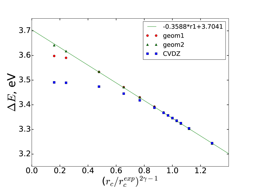
Figure 1: Calculated dependence of the hyperfine splitting, $\Delta E$, of the ground electronic state of the hydrogen like ²⁰⁵Tl on $r_{c}^{2\gamma-1}$ in the point nuclear magnetic dipole moment model in different basis sets (see text). $r_{c}$ is the nuclear charge radius.

Figs. 2 and 3 give calculated dependence of hyperfine splittings of the ground electronic state of the hydrogen like ²⁰³Tl and ²⁰⁵Tl on magnetic radii. Horizontal lines show the experimental energy splitting with the corresponding uncertainty taken from Ref. Beiersdorfer et al. (2001). From these data it is possible to fix magnetic radii for the used model of the magnetization distribution. For ²⁰⁵Tl one obtains $r_{m}/r_{c}^{exp}=$ 1.109(2) and for ²⁰³Tl $r_{m}/r_{c}^{exp}=$ 1.104(2).

Combining theoretical and experimental data, the coefficients $d_{nuc}=1.17$ for ²⁰³Tl and $d_{nuc}=1.18$ for ²⁰⁵Tl were obtained for the parametrization given by Eq. (7).

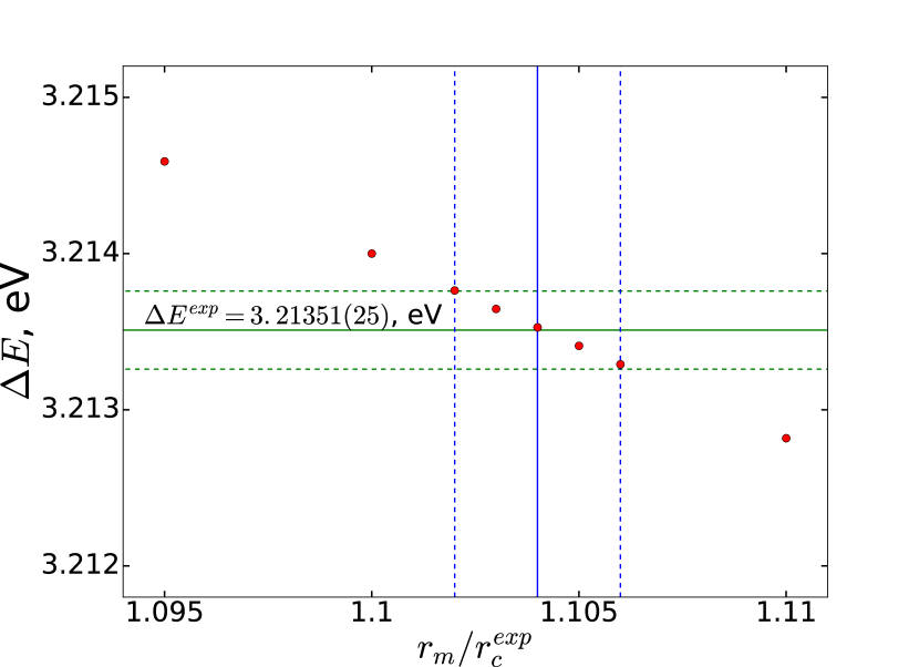
Figure 2: Calculated dependence of the hyperfine splitting ($\Delta E$) of the ground electronic state of the hydrogen like ²⁰³Tl on the ratio $r_{m}/r_{c}^{exp}$ of the magnetic radius $r_{m}$ and experimental charge radius $r_{c}^{exp}$. Solid and dashed horizontal lines show the experimental energy splitting value with the corresponding uncertainty from Ref. Beiersdorfer et al. (2001). Vertical lines show the extracted magnetic radius with the corresponding uncertainty.

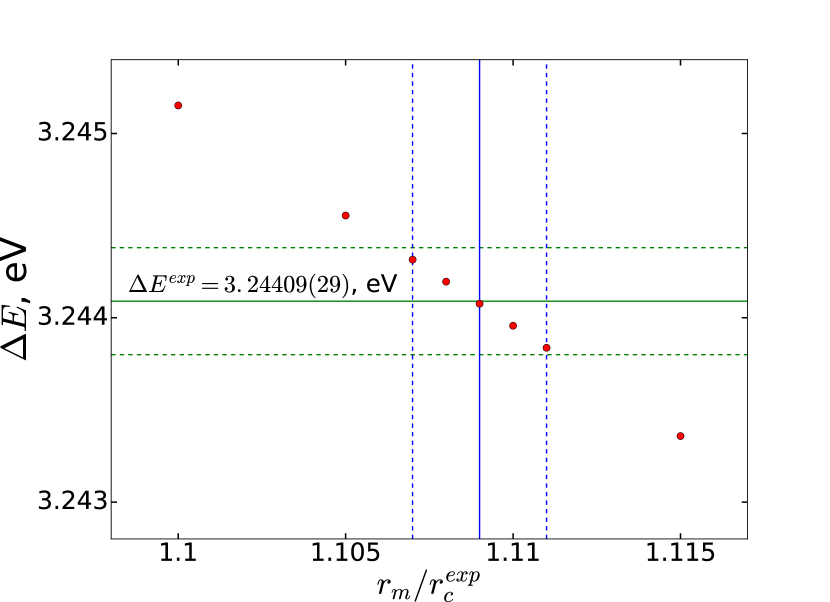
Figure 3: Calculated dependence of the hyperfine splitting ($\Delta E$) of the ground electronic state of the hydrogen like ²⁰⁵Tl on the ratio $r_{m}/r_{c}^{exp}$ of the magnetic radius $r_{m}$ and experimental charge radius $r_{c}^{exp}$. Solid and dashed horizontal lines show the experimental energy splitting value with the corresponding uncertainty from Ref. Beiersdorfer et al. (2001). Vertical lines show the extracted magnetic radius with the corresponding uncertainty.

IV.2 Neutral thallium ²⁰⁵Tl in $6P_{1/2}$ state

Table 1 gives calculated values of the ²⁰⁵Tl hyperfine structure constant for the $6P_{1/2}$ state for a number of magnetic radii. The last column gives values for $r_{m}/r_{c}^{exp}=1.11$ which is close to the value obtained from the analysis given above for the hyperfine splitting in the hydrogen like ²⁰⁵Tl.

$r_{m}/r_{c}^{exp}$	0	1	1.1	1.11
DHF	18805	18681	18660	18658
CCSD	21965	21807	21781	21778
CCSD(T)	21524	21372	21347	21345
+Basis corr.	-21	-21	-21	-21
+CCSDT-CCSD(T)	+73	+73	+73	+73
+CCSDT(Q)-CCSDT	-5	-5	-5	-5
+Gaunt	-83	-83	-83	-83
Total	21488	21337	21312	21309

Table 1: Calculated values of the hyperfine structure constant of the $6P_{1/2}$ state of ²⁰⁵Tl (in MHz) at different levels of theory.

The final value for the HFS constant with accounting for the Bohr-Weisskopf correction is 21309 MHz and is in a very good agreement with the experimental value 21310.8 MHz Lurio and Prodell (1956) and previous studies (see Table 4). One can estimate the theoretical uncertainty of the calculated HFS constant to be smaller than 1%.

IV.3 Neutral thallium ²⁰⁵Tl in $6P_{3/2}$ state

Table 2 gives calculated values of the HFS constant for the $6P_{3/2}$ state of the ²⁰⁵Tl atom. One can see that correlation effects dramatically contribute to the constant. This has also been noted in previous studies of this state Konovalova et al. (2017); Mårtensson-Pendrill (1995). Interestingly that even quadruple cluster amplitudes give non-negligible relative contribution to the HFS constant.

$r_{m}/r_{c}^{exp}$	0	1	1.1	1.11
DHF	1415	1415	1415	1415
CCSD	6	40	46	47
CCSD(T)	244	273	278	278
+Basis corr.	+4	+4	+4	+4
+CCSDT-CCSD(T)	-49	-49	-49	-49
+CCSDT(Q)-CCSDT	+13	+13	+13	+13
+Gaunt	+1	+1	+1	+1
Total	214	243	248	248

Table 2: Calculated values of the hyperfine structure constant of the $6P_{3/2}$ state of ²⁰⁵Tl (in MHz) at different levels of theory

Calculated value of the BW correction to the HFS constant of the $6P_{3/2}$ state of ²⁰⁵Tl is $-$16%. It has an opposite sign with respect to the BW correction to the HFS constant of the $6P_{1/2}$ (see Table 3).

$r_{m}/r_{c}^{exp}$	1	1.1	1.11
$6P_{1/2}$	0.0070	0.0082	0.0083
$6P_{3/2}$	-0.14	-0.16	-0.16

Table 3: Calculated values of the Bohr-Weisskopf correction to the hyperfine structure constants of the $6P_{1/2}$ and $6P_{3/2}$ states of ²⁰⁵Tl for different values of the $r_{m}/r_{c}^{exp}$ ratio.

Author, Ref.	$6P_{1/2}$	$6P_{3/2}$
Kozlov et al. Kozlov et al. (2001)	21663	248
Safronova et al. Safronova et al. (2005)	21390	353
Mårtensson-Pendrill Mårtensson-Pendrill (1995)	20860	256
This work	21488	214

Table 4: Total values of hyperfine structure constants in the point nuclear magnetic dipole moment model for ²⁰⁵Tl (in MHz) in comparison with previous studies.

Obtained value of the HFS constant is in a reasonable agreement with the experimental value 265 MHz Gould (1956). Theoretical uncertainty of the final value can be estimated as 10%. Note, however, that it corresponds to about 2% of the total correlation contribution – compare the final value with the Dirac-Hartree Fock (DHF) value.

V Hyperfine anomaly

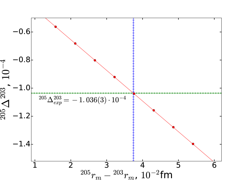
Figure 4: Calculated dependence of the $6P_{1/2}$ hyperfine anomaly ${}^{205}\Delta^{203}$ on the difference of magnetic radii ${}^{205}r_{m}-{}^{203}r_{m}$. Solid and dashed horizontal lines indicate the experimental value and its uncertainty; calculated values are given by circles and vertical lines give the value of the magnetic radii difference and its uncertainty.

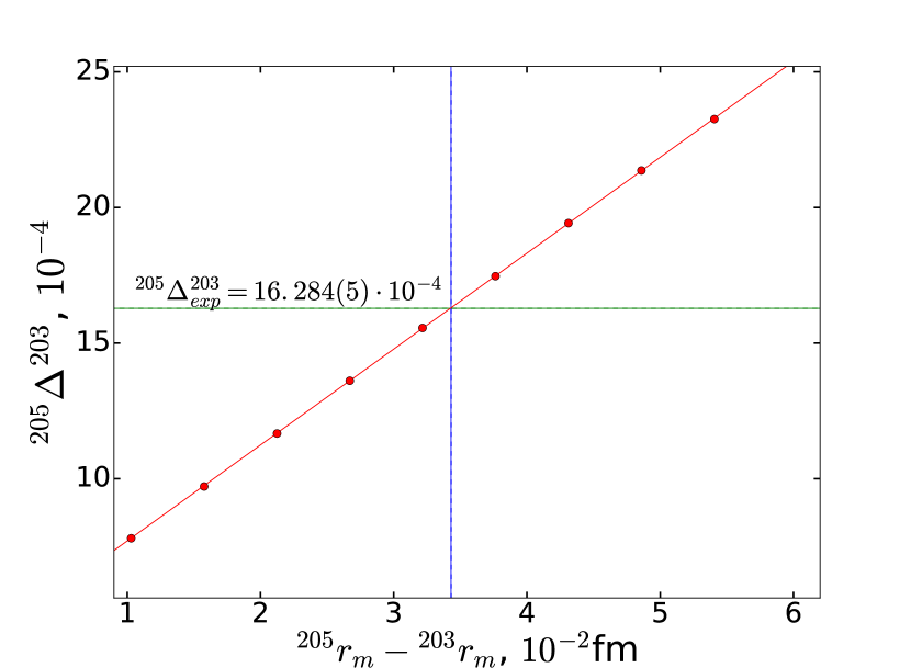
Figure 5: Calculated dependence of the $6P_{3/2}$ hyperfine anomaly ${}^{205}\Delta^{203}$ on the difference of magnetic radii ${}^{205}r_{m}-{}^{203}r_{m}$. Solid and dashed horizontal lines indicate the experimental value and its uncertainty; calculated values are given by circles and vertical lines give the value of the magnetic radii difference and its uncertainty.

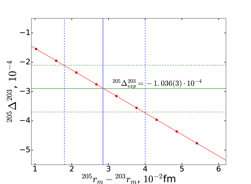
Figure 6: Calculated dependence of the $7S_{1/2}$ hyperfine anomaly ${}^{205}\Delta^{203}$ on the difference of magnetic radii ${}^{205}r_{m}-{}^{203}r_{m}$. Solid and dashed horizontal lines indicate the experimental value and its uncertainty; calculated values are given by circles and vertical lines give the value of the magnetic radii difference and its uncertainty.

Magnetic moments of ²⁰³Tl and ²⁰⁵Tl are known with a good accuracy Stone (2005). Values of HFS constants of the $6P_{1/2}$, $6P_{3/2}$ and $7S_{1/2}$ states have been measured precisely in Refs. Lurio and Prodell (1956); Gould (1956); Chen et al. (2012). Thus, experimental values of the magnetic anomalies ${}^{205}\Delta^{203}$ for these states are also known with a high precision. Figs. 4, 5 and 6 show calculated dependence of the values of anomalies for these states on the difference of magnetic radii ${}^{205}r_{m}-{}^{203}r_{m}$. In these calculations charge radii of ²⁰³Tl and ²⁰⁵Tl were set to experimental values. Calculations were performed within the CCSD(T) method in the MBas basis set. In Figs. 4, 5 and 6 solid and dashed horizontal lines show the experimental value and its uncertainty. By considering the intersection of the calculated (without treatment of the QED effects) dependence (which is approximated by linear functions) with horizontal dashed lines one obtains the difference of magnetic radii ${}^{205}r_{m}-{}^{203}r_{m}$ and its uncertainty in the model under consideration.

One can see from Figs. 4 and 5 that the differences extracted from the data for the $6P_{1/2}$ and $6P_{3/2}$ states agree within 10% which confirms the applicability of the model under consideration. They are also in a good agreement with the difference obtained from the data for the $7S_{1/2}$ state of the neutral Tl as well as from the data for the hydrogen like Tl above — within the experimental uncertainty for these systems.

VI Magnetic moments of short lived isotopes

Magnetic anomalies can be used to determine the value of the nuclear magnetic moment of the short lived isotope (for example see Refs. Cheal and Flanagan (2010); Schmidt et al. (2018); Barzakh et al. (2012)). For this one should know the nuclear magnetic moment value of the stable isotope as well as HFS constants ($A[a]$ and $A[b]$) for two electronic states ($a$ and $b$) of this isotope and the short lived isotope. Consider isotopes 1 (²⁰⁵Tl, $I=1/2$) and 2 (¹⁹³Tl, $I=9/2$). The latter is unstable. From the experimental data Barzakh et al. (2012); Lurio and Prodell (1956); Chen et al. (2012) one obtains:

$${}^{1}\theta^{2}[a,b]=\frac{A_{1}[a]}{A_{2}[b]}\frac{A_{2}[a]}{A_{1}[b]}-1=-0.013(7).$$ (9)

Here $a=7S_{1/2}$, $b=6P_{1/2}$. Calculated value of the ratio of magnetic anomalies for these states is ${}^{1}k^{2}[a,b]={}^{1}\Delta^{2}[a]/{}^{1}\Delta^{2}[b]=3.4(2)$. Such ratio depends only slightly on the nuclear magnetization distribution model Cheal and Flanagan (2010); Schmidt et al. (2018). Now one obtains for the nuclear magnetic moment $\mu_{2}$ of the isotope 2:

$$\mu_{2}=\mu_{1}\cdot\frac{A_{2}[b]}{A_{1}[b]}\cdot\frac{I_{2}}{I_{1}}\cdot(1+{}^{1}\Delta^{2}[b])=3.84(3).$$ (10)

Using the same method and experimental data from Refs. Barzakh et al. (2012); Lurio and Prodell (1956); Chen et al. (2012) one obtains the nuclear magnetic moment value of the ¹⁹¹Tl isotope with nuclear spin $I=9/2$: $\mu_{191}=+3.79(2)$. Obtained values of $\mu_{191}$ and $\mu_{193}$ are in a very good agreement with Ref. Barzakh et al. (2012): $\mu_{193}=+3.82(3)$ and $\mu_{191}=+3.78(2)$.

VII Conclusion

In the present paper the Bohr-Weisskopf effect has been calculated for the $6P_{1/2}$, $6P_{3/2}$ and $7S_{1/2}$ states for several isotopes of the Tl atom. The uniformly magnetized ball model has been tested and used.

It was found that the correlation effects strongly contribute to the HFS constant (they are about 470% of the final value) as well as to the BW effect for the $6P_{3/2}$ state. BW correction for the $6P_{3/2}$ state was found to be about $-$16%. Such a significant contribution makes it possible to test models of the nuclear magnetization distribution.

Combining obtained theoretical values of magnetic anomalies and available experimental data nuclear magnetic moments of short-lived ¹⁹¹Tl and ¹⁹³Tl isotopes were predicted and found to be in a good agreement with the previous study Barzakh et al. (2012).

It was demonstrated that for such calculations the Gaussian basis sets can be used. Thus, the applied method can be extended to the calculation of the BW effect in molecules.

For the calculated value of the HFS constant of the $6P_{1/2}$ state a very good agreement with the experiment and the small theoretical uncertainty has been obtained. A further improvement can be achieved by the treatment of the QED effects contribution.

VIII Acknowledgment

We are grateful to Prof. M. Kozlov, Prof. I. Mitropolsky and Dr. Yu. Demidov for helpful discussions. Electronic structure calculations were performed at the PIK data center of NRC “Kurchatov Institute” – PNPI.

References

- Barzakh et al. (2013) A. Barzakh, L. K. Batist, D. Fedorov, V. Ivanov, K. Mezilev, P. Molkanov, F. Moroz, S. Y. Orlov, V. Panteleev, and Y. M. Volkov, Physical Review C 88, 024315 (2013).
- Barzakh et al. (2017) A. Barzakh, A. Andreyev, T. E. Cocolios, R. De Groote, D. Fedorov, V. Fedosseev, R. Ferrer, D. Fink, L. Ghys, M. Huyse, et al., Physical Review C 95, 014324 (2017).
- Beiersdorfer et al. (2001) P. Beiersdorfer, S. B. Utter, K. L. Wong, J. R. C. López-Urrutia, J. A. Britten, H. Chen, C. L. Harris, R. S. Thoe, D. B. Thorn, E. Träbert, et al., Phys. Rev. A 64, 032506 (2001).
- Schmidt et al. (2018) S. Schmidt, J. Billowes, M. Bissell, K. Blaum, R. G. Ruiz, H. Heylen, S. Malbrunot-Ettenauer, G. Neyens, W. Nörtershäuser, G. Plunien, et al., Physics Letters B 779, 324 (2018).
- Petrov et al. (2013) A. N. Petrov, L. V. Skripnikov, A. V. Titov, and R. J. Mawhorter, Phys. Rev. A 88, 010501(R) (2013).
- Mawhorter et al. (2011) R. J. Mawhorter, B. S. Murphy, A. L. Baum, T. J. Sears, T. Yang, P. Rupasinghe, C. McRaven, N. Shafer-Ray, L. D. Alphei, and J.-U. Grabow, Phys. Rev. A 84, 022508 (2011).
- Ginges and Flambaum (2004) J. S. M. Ginges and V. V. Flambaum, Phys. Rep. 397, 63 (2004).
- Safronova et al. (2018) M. Safronova, D. Budker, D. DeMille, D. F. J. Kimball, A. Derevianko, and C. W. Clark, Rev. Mod. Phys. 90, 025008 (2018).
- Skripnikov et al. (2014) L. V. Skripnikov, A. D. Kudashov, A. N. Petrov, and A. V. Titov, Phys. Rev. A 90, 064501 (2014).
- Skripnikov (2017) L. V. Skripnikov, J. Comp. Phys. 147, 021101 (2017).
- Ginges and Volotka (2018) J. Ginges and A. Volotka, Phys. Rev. A 98, 032504 (2018).
- Rosenthal and Breit (1932) J. E. Rosenthal and G. Breit, Physical Review 41, 459 (1932).
- Crawford (1949) M. Crawford, Phys. Rev. 76, 1310 (1949).
- Bohr and Weisskopf (1950) A. Bohr and V. Weisskopf, Physical Review 77, 94 (1950).
- Bohr (1951) A. Bohr, Phys. Rev. 81, 134 (1951).
- Mårtensson-Pendrill (1995) A.-M. Mårtensson-Pendrill, Physical review letters 74, 2184 (1995).
- Konovalova et al. (2017) E. Konovalova, M. Kozlov, Y. A. Demidov, and A. Barzakh, arXiv preprint arXiv:1703.10048 (2017).
- Gomez et al. (2008) E. Gomez, S. Aubin, L. Orozco, G. Sprouse, E. Iskrenova-Tchoukova, and M. Safronova, Physical review letters 100, 172502 (2008).
- Ginges et al. (2017) J. Ginges, A. Volotka, and S. Fritzsche, Phys. Rev. A 96, 062502 (2017).
- Dzuba (1984) V. Dzuba, J. Phys. B 17, 1953 (1984).
- Cheal and Flanagan (2010) B. Cheal and K. T. Flanagan, Journal of Physics G: Nuclear and Particle Physics 37, 113101 (2010), URL http://stacks.iop.org/0954-3899/37/i=11/a=113101.
- Barzakh et al. (2012) A. Barzakh, L. K. Batist, D. Fedorov, V. Ivanov, K. Mezilev, P. Molkanov, F. Moroz, S. Y. Orlov, V. Panteleev, and Y. M. Volkov, Physical Review C 86, 014311 (2012).
- Shabaev (1994) V. Shabaev, Journal of Physics B: Atomic, Molecular and Optical Physics 27, 5825 (1994).
- Shabaev et al. (1997) V. Shabaev, M. Tomaselli, T. Kühl, A. Artemyev, and V. Yerokhin, Phys. Rev. A 56, 252 (1997).
- Ionesco-Pallas (1960) N. Ionesco-Pallas, Physical Review 117, 505 (1960).
- Konovalova et al. (2018) E. A. Konovalova, Y. A. Demidov, M. G. Kozlov, and A. E. Barzakh, Atoms 6 (2018), ISSN 2218-2004, URL http://www.mdpi.com/2218-2004/6/3/39.
- Angeli and Marinova (2013) I. Angeli and K. Marinova, Atomic Data and Nuclear Data Tables 99, 69 (2013), ISSN 0092-640X, URL http://www.sciencedirect.com/science/article/pii/S0092640X12000265.
- Stone (2005) N. Stone, Atomic Data and Nuclear Data Tables 90, 75 (2005).
- Dyall (2006) K. G. Dyall, Theor. Chem. Acc. 115, 441 (2006).
- Dyall (1998) K. G. Dyall, Theor. Chem. Acc. 99, 366 (1998).
- Bartlett and Musiał (2007) R. J. Bartlett and M. Musiał, Reviews of Modern Physics 79, 291 (2007).
- Dyall (2012) K. G. Dyall, Theor. Chem. Acc. 131, 1217 (2012).
- Skripnikov et al. (2017) L. V. Skripnikov, D. E. Maison, and N. S. Mosyagin, Phys. Rev. A 95, 022507 (2017).
- (34) DIRAC, a relativistic ab initio electronic structure program, Release DIRAC15 (2015), written by R. Bast, T. Saue, L. Visscher, and H. J. Aa. Jensen, with contributions from V. Bakken, K. G. Dyall, S. Dubillard, U. Ekstroem, E. Eliav, T. Enevoldsen, E. Fasshauer, T. Fleig, O. Fossgaard, A. S. P. Gomes, T. Helgaker, J. Henriksson, M. Ilias, Ch. R. Jacob, S. Knecht, S. Komorovsky, O. Kullie, J. K. Laerdahl, C. V. Larsen, Y. S. Lee, H. S. Nataraj, M. K. Nayak, P. Norman, G. Olejniczak, J. Olsen, Y. C. Park, J. K. Pedersen, M. Pernpointner, R. Di Remigio, K. Ruud, P. Salek, B. Schimmelpfennig, J. Sikkema, A. J. Thorvaldsen, J. Thyssen, J. van Stralen, S. Villaume, O. Visser, T. Winther, and S. Yamamoto (see http://www.diracprogram.org).
- (35) mrcc, a quantum chemical program suite written by M. Kállay, Z. Rolik, I. Ladjánszki, L. Szegedy, B. Ladóczki, J. Csontos, and B. Kornis. See also Z. Rolik and M. Kállay, J. Chem. Phys. 135, 104111 (2011), as well as: www.mrcc.hu.
- Kállay and Surján (2001) M. Kállay and P. R. Surján, J. Comp. Phys. 115, 2945 (2001).
- Kállay et al. (2002) M. Kállay, P. G. Szalay, and P. R. Surján, J. Comp. Phys. 117, 980 (2002).
- Skripnikov (2016) L. V. Skripnikov, J. Comp. Phys. 145, 214301 (2016).
- Maison et al. (2018) D. E. Maison, L. V. Skripnikov, and D. A. Glazov, arXiv preprint arXiv:1811.07986 (2018).
- Lurio and Prodell (1956) A. Lurio and A. Prodell, Physical Review 101, 79 (1956).
- Kozlov et al. (2001) M. Kozlov, S. Porsev, and W. Johnson, Phys. Rev. A 64, 052107 (2001).
- Safronova et al. (2005) U. Safronova, M. Safronova, and W. Johnson, Phys. Rev. A 71, 052506 (2005).
- Gould (1956) G. Gould, Physical Review 101, 1828 (1956).
- Chen et al. (2012) T.-L. Chen, I. Fan, H.-C. Chen, C.-Y. Lin, S.-E. Chen, J.-T. Shy, and Y.-W. Liu, Phys. Rev. A 86, 052524 (2012).