A non-singular continuum theory of point defects using gradient elasticity of bi-Helmholtz type

Abstract

In this paper, we develop a non-singular continuum theory of point defects based on a second strain gradient elasticity theory, the so-called gradient elasticity of bi-Helmholtz type. Such a generalized continuum theory possesses a weak nonlocal character with two internal material lengths and provides a mechanics of defects without singularities. Gradient elasticity of bi-Helmholtz type gives a natural and physical regularization of the classical singularities of defects, based on higher order partial differential equations. Point defects embedded in an isotropic solid are considered as eigenstrain problem in gradient elasticity of bi-Helmholtz type. Singularity-free fields of point defects are presented. The displacement field as well as the first, the second and the third gradients of the displacement are derived and it is shown that the classical singularities are regularized in this framework. This model delivers non-singular expressions for the displacement field, the first displacement gradient and the second displacement gradient. Moreover, the plastic distortion (eigendistortion) and the gradient of the plastic distortion of a dilatation centre are also non-singular and are given in terms of a form factor (shape function) of a point defect. Singularity-free expressions for the interaction energy and the interaction force between two dilatation centres and for the interaction energy and the interaction force of a dilatation centre in the stress field of an edge dislocation are given. The results are applied to calculate the finite self-energy of a dilatation centre.

1 Introduction

Among the important problems widely addressed in the mechanics of defects is the determination of the elastic state of point defects. Defects (dislocations and point defects) are always present in crystalline solids. The interaction between defects can change considerably many properties of crystals. In addition to dislocations, which are line defects, point defects are also important defects in crystals [1, 2, 3]. Point defects can exist in different configurations such as vacancies, interstitials, substitutional atoms, and foreign atoms. The fields of point defects play an important role in determining the physical properties of solids. They cause volume change and interact with dislocations if dislocations climb. Point defects play a major role in many physical problems such as X-ray scattering, internal friction phenomena, aggregation of defects, dislocation locking and various diffusion processes [4, 1]. Nowadays, the fields caused by point defects are important in computer simulations of defect mechanics and discrete dislocation dynamics. Atomistic and ab initio simulations of point defects and their interaction with dislocations, including a comparison between atomic simulations and classical elasticity theory, are reported in [5, 6, 7].

Using the theory of classical elasticity, the displacement field and the elastic strain of point defects possess a $1/R^{2}$-singularity and a $1/R^{3}$-singularity, respectively [2]. Moreover, the elastic strain of a point defect possesses a Dirac $\delta$-singularity [8, 9, 10]. Such singularities are the result that classical elasticity is not valid at the small scale near defects. Therefore, nonlocal elasticity or strain gradient elasticity should be used in order to obtain non-singular fields of point defects in the close vicinity of the defect.

A particular version of Eringen’s theory of nonlocal elasticity [11] was used by Kovács [12], Wang [13] and Povstenko [14] to obtain non-singular stress fields whereas the displacement and elastic strain fields still possess the classical singularities. Gairola [15, 16] studied the elastic interaction between point defects using the nonlocal theory of elasticity. Vörös and Kovács [17, 18] investigated the elastic interaction between point defects and dislocations in a Debye quasi-continuum.

On the other hand, dilatation point defects (dilatation centres) were investigated by Adler [19] in the framework of Toupin-Mindlin’s first strain gradient elasticity [20, 21]. It was shown by Adler [19] by using the linearized form of Toupin’s strain-gradient theory [20] that in an isotropic material the displacement field produced by a dilatation point defect contains, besides the classical $1/R^{2}$-term, only exponentially decreasing contributions and the expression given in [19] is singular. Later, in a simplified gradient elasticity theory, Dobovšeck [22] showed that the displacement field of a dilatation point defect is non-singular and finite, but the strain and the strain gradient are still singular, but weaker singular than the classical singularities. Vlasov [23] studied the elastic interaction between point defects and dislocations using a theory of simplified strain gradient elasticity. Theory of first strain gradient elasticity is unable to regularize and to remove all the classical singularities appearing in the elastic fields of point defects. Therefore, strain gradient elasticity of higher order is needed for a realistic modelling of point defects described by singularity-free elastic fields. Moreover, using a simple version of Toupin’s theory of gradient elasticity at finite strains with only one gradient term, Wang et al. [24] obtained numerical solutions of a dilatation centre reproducing a non-singular and finite displacement field like in the linear theory of strain gradient elasticity obtained in [22].

Furthermore, second strain gradient elasticity theory (or gradient elasticity of grade-3) had originally been introduced by Mindlin [25, 26] (see also [27, 28, 29]). For the isotropic case, Mindlin’s theory of second strain gradient elasticity involves sixteen additional material constants (including a so-called modulus of cohesion), in addition to the two Lamé constants. These material constants give rise to four characteristic length scales. Gradient elasticity of grade-$n$ can be considered as the continuum version of a lattice theory with $n$th-neighbour interactions [25, 28]. In this way, Mindlin [25] connected second strain gradient elasticity (gradient elasticity of grade-3) with a one-dimensional lattice theory with first, second and third neighbour interactions (see also [30]).

Neglecting the modulus of cohesion and the coupling terms between the strain tensor and the second strain gradient tensor, a simplified and robust version of Mindlin’s second strain gradient elasticity, the so-called gradient elasticity theory of bi-Helmholtz type, was introduced by Lazar et al. [31] (see also [32, 33, 34]) and applied to problems of straight dislocations [31, 35], dislocation loops [36], straight disclinations [37] and cracks of mode I, II and III [38, 39]. Lazar et al. [31, 35] have shown that all physical state quantities of screw and edge dislocations are non-singular in this framework. Using gradient elasticity of bi-Helmholtz type, it is possible to eliminate not only the singularities of the strain and stress tensors, but also the singularities of the double and triple stress tensors and of the dislocation density tensors of straight dislocations. All fields calculated in the theory of gradient elasticity of bi-Helmholtz type are smoother than those calculated in gradient elasticity theory of Helmholtz type. The non-singular dislocation densities of screw and edge dislocations obtained by Lazar et al. [35, 31] in the framework of gradient elasticity of bi-Helmholtz type have been recently used by Lyu and Li [40] in the multiscale modelling of dislocation pattern dynamics. Gradient elasticity of bi-Helmholtz type is able to retain the main physical and mathematical features of Mindlin’s second strain gradient elasticity. Moreover, gradient elasticity of bi-Helmholtz type corresponds to nonlocal elasticity of bi-Helmholtz type with a nonlocal kernel being the Green function of a differential operator of fourth order of bi-Helmholtz type [31, 41]. The Cauchy stress in gradient elasticity of bi-Helmholtz type and the stress in nonlocal elasticity of bi-Helmholtz type give coinciding and non-singular solutions. Under specific assumptions for the characteristic material lengths, the dispersion relation of nonlocal elasticity of bi-Helmholtz type coincides with the dispersion relation of the Born-Kármán model without lacking thermodynamic consistency [11, 31, 42].

It should be noted that the influence of the coupling between the strain and the second strain gradient in Mindlin’s strain gradient theory and a simplified version of it has been recently studied for one-dimensional problems of nano-objects in [43, 44].

In this paper, we solve the long-outstanding problem of point defects in second strain gradient elasticity, in order to find non-singular fields produced by point defects. We will answer the important mathematical question, up to which order $n$ of singularity $1/R^{n}$, strain gradient elasticity of bi-Helmholtz type is able to regularize the classical singularities and leading to singularity-free expressions in 3D.

The outline of this paper is as follows: first, in Section 2 the theory of gradient elasticity of bi-Helmholtz type, including Green functions, parameter study of the two appearing characteristic material lengths and operator split, is presented. The problem of point defects is modelled as eigenstrain problem in second strain gradient elasticity of bi-Helmholtz type. In Section 3, the fields of a dilatation centre are computed and compared for gradient elasticity of bi-Helmholtz type, gradient elasticity of Helmholtz type and classical incompatible elasticity. The interaction between two dilatation centres and the interaction between an edge dislocation and a dilatation centre is studied in Section 4. We finally conclude in Section 5.

2 Gradient elasticity of bi-Helmholtz type

In this section, we consider the necessary basics, the three-dimensional Green tensor and the operator split of the theory of incompatible gradient elasticity of bi-Helmholtz type originally proposed by Lazar et al. [31] and we show that it is a suitable framework for a non-singular theory of point detects.

2.1 Basics of gradient elasticity of bi-Helmholtz type

Consider an infinite elastic body in a three-dimensional space and assume that the gradient of the displacement field $\bm{u}$ is additively decomposed into an elastic distortion tensor $\bm{\beta}$ and an inelastic distortion tensor (or eigendistortion tensor) $\bm{\beta}^{\mathrm{P}}$:

$$\partial_{j}u_{i}=\beta_{ij}+\beta^{\mathrm{P}}_{ij}\,.$$ (1)

For point defects, the eigendistortion tensor is often called quasi-plastic distortion tensor [45, 46]. The quasi-plastic distortion may serve as a defect density in its own right. As mentioned by Kröner [47, 48, 49] and deWit [50] the plastic distortion $\bm{\beta}^{\mathrm{P}}$ of a point defect can be regarded as equivalent to an “infinitesimal dislocation loop density” being a fictitious dislocation distribution. The elastic strain tensor, $e_{ij}$, is the symmetric part of the elastic distortion tensor $\beta_{ij}$:

$$e_{ij}=\frac{1}{2}\left(\beta_{ij}+\beta_{ji}\right)\,.$$ (2)

In the linear theory of gradient elasticity of bi-Helmholtz type, the strain energy density $\mathcal{W}$ of an isotropic material is given by [32, 31, 36]

$$\mathcal{W}=\frac{1}{2}\,C_{ijkl}e_{ij}e_{kl}+\frac{1}{2}\,\ell_{1}^{2}C_{ijkl}\partial_{m}e_{ij}\partial_{m}e_{kl}+\frac{1}{2}\,\ell_{2}^{4}C_{ijkl}\partial_{n}\partial_{m}e_{ij}\partial_{n}\partial_{m}e_{kl}\,,$$ (3)

where $\ell_{1}$ and $\ell_{2}$ are the two characteristic material lengths of gradient elasticity of bi-Helmholtz type and $C_{ijkl}$ is the tensor of elastic moduli. In gradient elasticity of bi-Helmholtz type, the strain energy density (3) is given in terms of three contributions, each one quadratic in elastic strain, first strain gradient and second strain gradient. Eq. (3) can be derived from the form II of Mindlin’s anisotropic second strain gradient elasticity theory as a simplified version [31]. For isotropic materials, the tensor of elastic moduli reads

$$C_{ijkl}=\lambda\,\delta_{ij}\delta_{kl}+\mu\big{(}\delta_{ik}\delta_{jl}+\delta_{il}\delta_{jk}\big{)}\,,$$ (4)

where $\mu$ and $\lambda$ are the Lamé moduli. The condition for positive semidefiniteness of the strain energy density, $\mathcal{W}\geq 0$, gives

$$\ell_{1}^{2}\geq 0\,,\qquad\ell_{2}^{4}\geq 0\,,$$ (5)

in addition to $(2\mu+3\lambda)\geq 0$ and $\mu\geq 0$. The positive semidefiniteness is a necessary condition for stable material behaviour. If ${\cal W}$ is a quadratic form of its arguments, the strict convexity is equivalent to the positive definiteness, ${\cal W}>0$ (see also [43]).

The quantities canonically conjugated to the elastic strain tensor $e_{ij}$, the first strain gradient tensor (double strain) $\partial_{k}e_{ij}$ and the second strain gradient tensor (triple strain) $\partial_{l}\partial_{k}e_{ij}$ are the Cauchy stress tensor $\sigma_{ij}$, the double stress tensor $\tau_{ijk}$ and the triple stress tensor $\tau_{ijkl}$, respectively, and they give the following constitutive relations

$$\sigma_{ij} =\frac{\partial\mathcal{W}}{\partial e_{ij}}=C_{ijmn}e_{mn}\,,$$ (6)

$$\tau_{ijk} =\frac{\partial\mathcal{W}}{\partial(\partial_{k}e_{ij})}=\ell_{1}^{2}\,C_{ijmn}\partial_{k}e_{mn}=\ell_{1}^{2}\partial_{k}\sigma_{ij}\,,$$ (7)

$$\tau_{ijkl} =\frac{\partial\mathcal{W}}{\partial(\partial_{l}\partial_{k}e_{ij})}=\ell_{2}^{4}\,C_{ijmn}\partial_{l}\partial_{k}e_{mn}=\ell_{2}^{4}\partial_{l}\partial_{k}\sigma_{ij}\,,$$ (8)

where we used that the elastic moduli are constant for homogeneous media. Eq. (6) is nothing else than the Hooke law. It can be seen that $\ell_{1}$ is the characteristic length for the double stress tensor. On the other hand, $\ell_{2}$ is the characteristic length for the triple stress tensor. It is remarkable, that the double stress tensor (7) is nothing but the first gradient of the stress tensor multiplied by $\ell_{1}^{2}$, and that the triple stress tensor (8) is nothing but the second gradient of the stress tensor multiplied by $\ell_{2}^{4}$. For a deeper discussion of the physical meaning of the double and triple stresses we refer to [51]. Unlike Mindlin’s second strain gradient elasticity [25], no coupling terms appear in the constitutive equations (6)–(8) (see also [31]). However, a second strain gradient term in Eq. (6) could give singular contributions to the Cauchy stress tensor $\sigma_{ij}$ which would not give a non-singular continuum theory of point defects. A modulus of cohesion would just give a constant contribution to the triple stress tensor (8) being not relevant for the modelling of defects.

Using Eqs. (6)–(8), Eq. (3) can be re-written as [31]

$$\mathcal{W}=\frac{1}{2}\,\sigma_{ij}e_{ij}+\frac{1}{2}\,\ell_{1}^{2}\partial_{k}\sigma_{ij}\partial_{k}e_{ij}+\frac{1}{2}\,\ell_{2}^{4}\partial_{l}\partial_{k}\sigma_{ij}\partial_{l}\partial_{k}e_{ij}\,.$$ (9)

The strain energy density (9) exhibits a stress-strain symmetry in $\sigma_{ij}$ and $e_{ij}$, in $\partial_{k}\sigma_{ij}$ and $\partial_{k}e_{ij}$, and in $\partial_{l}\partial_{k}\sigma_{ij}$ and $\partial_{l}\partial_{k}e_{ij}$ (see also [32]). Using the inverse tensor of the elastic moduli $C_{ijkl}^{-1}$, the energy density (3) can be written in an equivalent stress gradient form

$$\mathcal{W}=\frac{1}{2}\,C^{-1}_{ijkl}\sigma_{ij}\sigma_{kl}+\frac{1}{2}\,\ell_{1}^{2}C^{-1}_{ijkl}\partial_{m}\sigma_{ij}\partial_{m}\sigma_{kl}+\frac{1}{2}\,\ell_{2}^{4}C^{-1}_{ijkl}\partial_{n}\partial_{m}\sigma_{ij}\partial_{n}\partial_{m}\sigma_{kl}\,.$$ (10)

An interesting side-remark, using Eqs. (9) and (10), we may define the quantities canonically conjugated to the Cauchy stress tensor, the first stress gradient tensor and the second stress gradient tensor which are the tensors $e_{ij}$, $\phi_{ijk}$ and $\phi_{ijkl}$, respectively, and they give the following inverse constitutive relations

$$e_{ij} =\frac{\partial\mathcal{W}}{\partial\sigma_{ij}}=C^{-1}_{ijmn}\sigma_{mn}\,,$$ (11)

$$\phi_{ijk} =\frac{\partial\mathcal{W}}{\partial(\partial_{k}\sigma_{ij})}=\ell_{1}^{2}\,C^{-1}_{ijmn}\partial_{k}\sigma_{mn}=\ell_{1}^{2}\partial_{k}e_{ij}\,,$$ (12)

$$\phi_{ijkl} =\frac{\partial\mathcal{W}}{\partial(\partial_{l}\partial_{k}\sigma_{ij})}=\ell_{2}^{4}\,C^{-1}_{ijmn}\partial_{l}\partial_{k}\sigma_{mn}=\ell_{2}^{4}\partial_{l}\partial_{k}e_{ij}\,.$$ (13)

Eq. (11) is simply the inverse Hooke law. It is remarkable that $\phi_{ijk}$ is nothing but the first gradient of the elastic strain tensor multiplied by $\ell_{1}^{2}$, and $\phi_{ijkl}$ is nothing but the second gradient of the elastic strain tensor multiplied by $\ell_{2}^{4}$. Since the strain $e_{ij}$ is dimensionless, $\phi_{ijk}$ has the dimension: [length], and $\phi_{ijkl}$ has the dimension: [length]². Such a tensor $\phi_{ijk}$ was originally introduced by Forest and Sab [52] as micro-displacement tensor in stress gradient continuum theory (see also [53]).
It is interesting to note that the symmetry between the constitutive relations (6)–(8) and the inverse constitutive relations (11)–(13) is based on the above mentioned symmetry between strains and stresses in the strain energy density (9) of gradient elasticity of bi-Helmholtz type.

In the presence of body forces $\bm{b}$, the static Lagrangian density reads

$$\mathcal{L} =-\mathcal{W}-\mathcal{V}\,,$$

where

$$\mathcal{V}=-u_{i}b_{i}$$ (14)

is the potential of body forces. The condition of static equilibrium is expressed by the Euler-Lagrange equations. In second strain gradient elasticity (linear elasticity of grade-3), the Euler-Lagrange equations read (e.g., [29])

$$\frac{\delta\mathcal{L}}{\delta u_{i}}=\frac{\partial\mathcal{L}}{\partial u_{i}}-\partial_{j}\,\frac{\partial\mathcal{L}}{\partial(\partial_{j}u_{i})}+\partial_{k}\partial_{j}\,\frac{\partial\mathcal{L}}{\partial(\partial_{k}\partial_{j}u_{i})}-\partial_{l}\partial_{k}\partial_{j}\,\frac{\partial\mathcal{L}}{\partial(\partial_{l}\partial_{k}\partial_{j}u_{i})}=0\,.$$ (15)

In terms of the Cauchy stress, double stress and triple stress tensors, Eq. (15) takes the form [25]

$$\partial_{j}(\sigma_{ij}-\partial_{k}\tau_{ijk}+\partial_{l}\partial_{k}\tau_{ijkl})+b_{i}=0\,.$$ (16)

Using Eqs. (7) and (8), Eq. (16) reduces to

$$L\,\partial_{j}\sigma_{ij}+b_{i}=0\,,$$ (17)

where the fourth order differential operator $L$ is given by

$$L=\big{(}1-\ell_{1}^{2}\Delta+\ell_{2}^{4}\Delta\Delta\big{)}\,,$$ (18)

where $\Delta$ is the Laplace operator.

Substituting the constitutive relation (6) and Eq. (1) into the equilibrium condition (17), we obtain a partial differential equation of sixth order, which is called bi-Helmholtz-Navier equation [31, 36], for the displacement vector ${\bm{u}}$

$$LL_{ik}u_{k}=C_{ijkl}\partial_{j}L\beta^{{\mathrm{P}}}_{kl}-b_{i}\,,$$ (19)

where

$$L_{ik}=C_{ijkl}\partial_{j}\partial_{l}$$ (20)

is the Navier differential operator. For an isotropic material, it reads

$$L_{ik}=\mu\,\delta_{ik}\Delta+(\mu+\lambda)\,\partial_{i}\partial_{k}\,.$$ (21)

Eq. (19) is nothing but the equilibrium condition (17) written in terms of the displacement vector ${\bm{u}}$ and the plastic distortion tensor $\bm{\beta}^{\mathrm{P}}$, and

$$f_{i}=b_{i}-C_{ijkl}\partial_{j}L\beta^{\mathrm{P}}_{kl}$$ (22)

is the body force-type term. Notice that the second term on the right hand side of Eq. (22) is an “effective” or “fictitious” internal body force due to the gradient of the eigendistortion, and arises in the presence of defects, such as point defects, dislocations, and disclinations. This term is the gradient version of the internal force in Mura’s eigenstrain method [54]. For defects, the body force density vanishes, $b_{i}=0$.

Alternatively, the differential operator of fourth order (18) can be written in the form as product of two Helmholtz operators (differential operators of second order)

$$L=\big{(}1-c_{1}^{2}\Delta\big{)}\big{(}1-c_{2}^{2}\Delta\big{)}$$ (23)

with

$$\ell_{1}^{2} =c_{1}^{2}+c_{2}^{2}\,,$$ (24)

$$\ell_{2}^{4} =c_{1}^{2}\,c_{2}^{2}\,$$ (25)

and

$$c^{2}_{1,2} =\frac{\ell_{1}^{2}}{2}\Bigg{(}1\pm\sqrt{1-4\,\frac{\ell_{2}^{4}}{\ell_{1}^{4}}}\Bigg{)}\,.$$ (26)

Here $c_{1}$ and $c_{2}$ are the two auxiliary lengths appearing in the two Helmholtz operators in Eq. (23). Due to its structure as a product of two Helmholtz operators, the differential operator (23) is called bi-Helmholtz operator [31, 41].

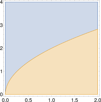
Figure 1: Parameter diagram for the cases (1), (2) and (3) in gradient elasticity of bi-Helmholtz type respecting the condition of positive semidefiniteness of the strain energy density for the material lengths $\ell_{1}$ and $\ell_{2}$: $\ell_{1}^{2}\geq 0$ and $\ell_{2}^{4}\geq 0$.

An important matter is the question concerning the mathematical character of the auxiliary lengths $c_{1}$ and $c_{2}$. In Mindlin’s theory of second strain gradient elasticity [25, 26], Mindlin [25] (see also [28]) pointed out that the conditions for positive $\mathcal{W}$ supply no indications of the character, real or complex, of the four auxiliary lengths $l_{11}$, $l_{21}$, $l_{12}$, $l_{22}$ of Mindlin’s second strain gradient elasticity. In the theory of gradient elasticity of bi-Helmholtz type, the condition for the character, real or complex, of the auxiliary lengths $c_{1}$ and $c_{2}$ can be obtained from the condition if in Eq. (26) the discriminant, $1-4\ell_{2}^{4}/\ell_{1}^{4}$, is positive or negative. We can distinguish three cases according to the sign of the discriminant:

• $\ell_{1}^{4}>4\ell_{2}^{4}$ :
  In this case, there are the two auxiliary lengths being real and distinct

  $$c_{1}^{2}\neq c_{2}^{2}\,.$$ (27)

  This case corresponds to region $\boxed{1}$ in Fig. 1. The auxiliary lengths $c_{1}$ and $c_{2}$ read as

  $$c_{1,2} =\sqrt{\frac{\ell_{1}^{2}}{2}\Bigg{(}1\pm\sqrt{1-4\,\frac{\ell_{2}^{4}}{\ell_{1}^{4}}}\Bigg{)}}\,.$$ (28)

  The limit to gradient elasticity of Helmholtz type is: $\ell_{2}^{4}\rightarrow 0$.

• $\ell_{1}^{4}=4\ell_{2}^{4}$ :
  There are the two auxiliary lengths being real and equal

  $$c_{1}^{2}=c_{2}^{2}=\frac{\ell_{1}^{2}}{2}\,.$$ (29)

  This case corresponds to the parabola $\boxed{2}$ in Fig. 1 defined according to $\ell_{1}^{4}=4\ell_{2}^{4}$. There is no limit to gradient elasticity of Helmholtz type.

• $\ell_{1}^{4}<4\ell_{2}^{4}$ :
  In this region, the two lengths $c_{1}^{2}$ and $c_{2}^{2}$ are complex conjugate

  $$c^{2}_{1,2} =\alpha\pm{\mathrm{i}}\beta\,$$ (30)

  with

  $$\alpha=\frac{\ell_{1}^{2}}{2}\qquad\text{and}\qquad\beta=\sqrt{\ell_{2}^{4}-\frac{\ell_{1}^{4}}{4}}\,.$$ (31)

  This case corresponds to region $\boxed{3}$ in Fig. 1. Moreover, the two auxiliary lengths $c_{1}$ and $c_{2}$ are also complex conjugate and read as

  $$c_{1,2} =A\pm{\mathrm{i}}B\,,$$ (32)

  where $A=\text{Re}\,(c_{1})=\text{Re}\,(c_{2})$ and $B=\text{Im}\,(c_{1})=-\text{Im}\,(c_{2})$. The original material lengths, $\ell_{1}$ and $\ell_{2}$ read in terms of $A$ and $B$

  $$\ell_{1}^{2} =2(A^{2}-B^{2})\,,$$ (33)

  $$\ell_{2}^{2} =A^{2}+B^{2}\,$$ (34)

  and the auxiliary lengths $c_{1}$ and $c_{2}$

  $$c^{2}_{1,2} =A^{2}-B^{2}\pm 2{\mathrm{i}}AB\,.$$ (35)

  Comparing Eq. (30) with Eq. (35), one gets

  $$\alpha=A^{2}-B^{2}\,,\qquad\beta=2AB\,.$$ (36)

  From the first part of the condition of positive semidefiniteness of the strain energy (5) and Eq. (33), we obtain

  $$A^{2}\geq B^{2}\,.$$ (37)

  Interesting to note that for the particular case $A^{2}=B^{2}$, it follows that $\ell_{1}^{2}=0$ and the first strain gradients disappear in the strain energy density (3). The corresponding strain gradient elasticity would be a gradient theory given only in terms of the strain and second strain gradient tensors. The cases $A^{2}<B^{2}$ and $A^{2}=0$ violate the first condition of positive semidefiniteness of the strain energy density (5). Moreover Eqs. (33) and (34) give

  $$A=\ell_{2}\,\sqrt{\frac{1}{2}+\frac{\ell_{1}^{2}}{4\ell_{2}^{2}}}\,,\qquad B=\ell_{2}\,\sqrt{\frac{1}{2}-\frac{\ell_{1}^{2}}{4\ell_{2}^{2}}}\,.$$ (38)

  For further calculations, it is convenient to introduce the inverse complex lengths

  $$c^{-1}_{1,2} =a\pm{\mathrm{i}}b$$ (39)

  with

  $$a=\frac{A}{A^{2}+B^{2}}=\frac{1}{\ell_{2}}\,\sqrt{\frac{1}{2}+\frac{\ell_{1}^{2}}{4\ell_{2}^{2}}}\,,\qquad b=-\frac{B}{A^{2}+B^{2}}=-\frac{1}{\ell_{2}}\,\sqrt{\frac{1}{2}-\frac{\ell_{1}^{2}}{4\ell_{2}^{2}}}\,.$$ (40)

  Since the auxiliary lengths $c_{1}$ and $c_{2}$ are complex conjugate, the characteristic material lengths $\ell_{1}$ and $\ell_{2}$ are real. The limit to gradient elasticity of Helmholtz type ($\ell_{2}^{4}\rightarrow 0$) leads to $\ell_{1}^{4}<0$, violating the condition of positive semidefiniteness of the strain energy density (5).

2.2 Parameter study

An important issue in strain gradient elasticity theories is the calculation of the characteristic lengths in addition to the elastic constants [55, 56, 57]. Zhang et al. [34] determined, in an atomistic calculation, the two auxiliary lengths $c_{1}$ and $c_{2}$ as positive and real for graphene. On the other hand, using the Sutton-Chen interatomic potential, Shodja et al. [58] calculated the values of the four auxiliary lengths $l_{11}$, $l_{21}$, $l_{12}$, $l_{22}$ of Mindlin’s second strain gradient elasticity for fcc crystals and found complex conjugate lengths. Using ab initio calculations, Ojaghnezhad and Shodja [59] obtained positive and real lengths of Mindlin’s second strain gradient elasticity. The two auxiliary lengths $c_{1}$ and $c_{2}$ of gradient elasticity of bi-Helmholtz type can be approximated from the four auxiliary lengths $l_{11}$, $l_{21}$, $l_{12}$, $l_{22}$ of Mindlin’s second strain gradient elasticity as

$$c_{1} =\frac{l_{11}+l_{21}}{2}\,,\qquad c_{2}=\frac{l_{12}+l_{22}}{2}\,.$$ (41)

The two auxiliary lengths $c_{1}$ and $c_{2}$ might be considered as the average of the four auxiliary lengths $l_{11}$, $l_{21}$ and $l_{12}$, $l_{22}$, respectively. $c_{1}^{2}$, $l^{2}_{11}$, $l_{21}^{2}$ correspond to the plus sign in front of the square root and $c_{2}^{2}$, $l^{2}_{12}$, $l_{22}^{2}$ correspond to the minus sign in front of the square root (see Eq. (26) and related expressions in [25, 58]). Therefore, we study the field solutions for the cases (1), (2) and (3).

Here, we provide the lengths used in this work in the numerical study of three-dimensional gradient elasticity of bi-Helmholtz type:
Case (1):

$$c_{1}=0.4\,a_{0}\,,\qquad c_{2}=0.2\,a_{0}$$ (42)

and

$$\ell_{1}=0.447\,a_{0}\,,\qquad\ell_{2}=0.283\,a_{0}\,,$$ (43)

where $a_{0}$ is the lattice constant of the material under consideration. This choice is motivated by atomistic calculations in first strain gradient elasticity [55, 57, 56] and by the value $\ell=0.4\,a_{0}$ found in the study of dispersion curves in Eringen’s nonlocal elasticity [60, 11].
Case (2):

$$c_{1}=c_{2}=\ell_{2}=\frac{\ell_{1}}{\sqrt{2}}=0.283\,a_{0}\,.$$ (44)

Case (3):

$$c_{1}=(0.250+0.197\,{\mathrm{i}})\,a_{0}\,,\qquad c_{2}=(0.250-0.197\,{\mathrm{i}})\,a_{0}$$ (45)

and

$$\ell_{1}=0.218\,a_{0}\,,\qquad\ell_{2}=0.318\,a_{0}\,.$$ (46)

This choice is motivated by atomistic calculations in Mindlin’s second strain gradient elasticity [58] and by the study of dispersion curves in nonlocal elasticity of bi-Helmholtz type [41]. Using the values (46), the dispersion curve in nonlocal elasticity of bi-Helmholtz type coincides with the one based on the Born-Kármán model (see [61, 11, 41]).

From the mathematical point of view, the lengths $\ell_{1}$, $\ell_{2}$ and $c_{1}$, $c_{2}$ play the role of regularization parameters in gradient elasticity of bi-Helmholtz type.

2.3 Green tensor of the three-dimensional bi-Helmholtz-Navier equation and relevant Green functions

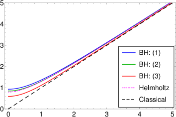
Figure 2: Plot of the auxiliary function $A(R)$.

The Green tensor of the three-dimensional bi-Helmholtz-Navier operator, $LL_{ik}$, is defined by

$$LL_{ik}G_{kj}({\bm{x}}-{\bm{x}}^{\prime})=-\delta_{ij}\delta({\bm{x}}-{\bm{x}}^{\prime})$$ (47)

and reads as [36]

$$G_{ij}(\bm{R})=\frac{1}{16\pi\mu(1-\nu)}\,\Big{[}2(1-\nu)\delta_{ij}\Delta-\partial_{i}\partial_{j}\Big{]}A(R)\,$$ (48)

with the auxiliary function for the Green tensor of the bi-Helmholtz-Navier operator for case (1)

$$A(R)=R+\frac{2(c_{1}^{2}+c_{2}^{2})}{R}-\frac{2}{c_{1}^{2}-c_{2}^{2}}\,\frac{1}{R}\Big{(}c_{1}^{4}\,{\mathrm{e}}^{-R/c_{1}}-c_{2}^{4}\,{\mathrm{e}}^{-R/c_{2}}\Big{)}\,,$$ (49)

where $R=|{\bm{x}}-{\bm{x}}^{\prime}|$ and $\nu$ is the Poisson ratio. The auxiliary function $A(R)$ may be regarded as a “regularized distance function”. In the far field, it is just $R$ and in the near field, it is modified due to gradient parts (second and third parts in Eq. (49)) (see Fig. 2).

In case (2), Eq. (49) simplifies to

$$A(R)=R+\frac{4c_{1}^{2}}{R}-\bigg{(}c_{1}+\frac{4c_{1}^{2}}{R}\bigg{)}\,{\mathrm{e}}^{-R/c_{1}}\,.$$ (50)

In case (3), using Eq. (30) and Euler’s formula, Eq. (49) reduces to

$$A(R)=R+\frac{4(A^{2}-B^{2})}{R}-\frac{{\mathrm{e}}^{-aR}}{R}\bigg{[}4(A^{2}-B^{2})\cos(bR)-\frac{A^{4}-6A^{2}B^{2}+B^{4}}{AB}\,\sin(bR)\bigg{]}\,,$$ (51)

where $A$ and $B$ are given in Eq. (38) and $a$ and $b$ are given in Eq. (40). The auxiliary function $A(R)$ is plotted for the cases (1), (2) and (3) in Fig. 2.

The Green tensor of the bi-Helmholtz-Navier equation is non-singular (see also [36]). Thus, Eq. (48) represents the regularized Green tensor in gradient elasticity of bi-Helmholtz type. Note that $A(R)$ can be written as the convolution of $R$ and $G^{\text{BH}}(R)$

$$A(R)=R*G^{\text{BH}}(R)\,,$$ (52)

where the symbol $*$ denotes the spatial convolution and $G^{\text{BH}}$ is the Green function of the three-dimensional bi-Helmholtz equation

$$LG^{\text{BH}}(R)=\delta({\bm{x}}-{\bm{x}}^{\prime})\,,$$ (53)

which reads for case (1) (e.g., [31])

$$G^{\text{BH}}(R)=\frac{1}{4\pi(c_{1}^{2}-c_{2}^{2})R}\,\Big{(}{\mathrm{e}}^{-R/c_{1}}-{\mathrm{e}}^{-R/c_{2}}\Big{)}\,.$$ (54)

It can be seen in Eq. (52) that $G^{\text{BH}}(R)$ plays the role of the regularization function in gradient elasticity of bi-Helmholtz type. $G^{\text{BH}}$ is a “mollifier” (e.g., [62]). From the physical point of view, $G^{\text{BH}}(R)$ characterizes the shape of the defect and is a form factor or shape function of the defect. The Green function (54) is non-singular and possesses a maximum value at $R=0$, namely

$$G^{\text{BH}}(0)=\frac{1}{4\pi c_{1}c_{2}(c_{1}+c_{2})}\,.$$ (55)

Moreover, the Green function (54) is a Dirac-delta sequence with parametric dependence $c_{1}$ and $c_{2}$

$$\lim_{c_{1}\to 0,\,c_{2}\to 0}G^{\text{BH}}(R)=\delta({\bm{R}})$$ (56)

and it plays the role of the “regularization Green function” in gradient elasticity of bi-Helmholtz type. The Green function (54) is plotted in Fig. 3(a).

In case (2), the Green function (54) simplifies to

$$G^{\text{BH}}(R)=\frac{1}{8\pi c_{1}^{3}}\,{\mathrm{e}}^{-R/c_{1}}\,,$$ (57)

possessing a maximum value at $R=0$

$$G^{\text{BH}}(0)=\frac{1}{8\pi c_{1}^{3}}\,.$$ (58)

In case (3), the Green function (54) reduces to

$$G^{\text{BH}}(R)=-\frac{1}{8\pi AB}\,\frac{{\mathrm{e}}^{-aR}}{R}\,\sin(bR)\,,$$ (59)

having a maximum value at $R=0$

$$G^{\text{BH}}(0)=\frac{1}{8\pi A(A^{2}+B^{2})}\,.$$ (60)

The Green function $G^{\text{BH}}(R)$ is plotted for the cases (1), (2) and (3) in Fig. 3(a).

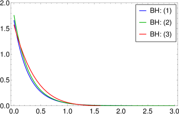
Figure 3: Plot of the Green function: (a) $G^{\text{BH}}(R)$ and (b) radial part of $\partial_{k}G^{\text{BH}}(R)$ for the cases (1), (2) and (3).

The gradient of the Green function (54) of the bi-Helmholtz equation is given by

$$\partial_{k}G^{\text{BH}}(R)=-\frac{1}{4\pi(c_{1}^{2}-c_{2}^{2})}\,\frac{R_{k}}{R^{3}}\bigg{[}{\mathrm{e}}^{-R/c_{1}}-{\mathrm{e}}^{-R/c_{2}}+\frac{R}{c_{1}}\,{\mathrm{e}}^{-R/c_{1}}-\frac{R}{c_{2}}\,{\mathrm{e}}^{-R/c_{2}}\bigg{]}\,.$$ (61)

Eq. (61) is non-singular and possesses a finite value at $R=0$, namely

$$\partial_{k}G^{\text{BH}}(0)=-\frac{1}{8\pi c^{2}_{1}c^{2}_{2}}\,\tau_{k}\,,$$ (62)

where $\tau_{k}=R_{k}/R$ are the components of the unit vector. The radial part of the gradient of the Green function (61) is plotted in Fig. 3(b). Moreover, the second gradient of the Green function (54), $\partial_{l}\partial_{k}G(R)$, leads to a singular expression (with $\frac{1}{R}$-singularity).

Moreover, in case (2) the gradient of the Green function (61) simplifies to

$$\partial_{k}G^{\text{BH}}(R)=-\frac{1}{8\pi c_{1}^{4}}\,\frac{R_{k}}{R^{3}}\,{\mathrm{e}}^{-R/c_{1}}\,.$$ (63)

In case (3) the gradient of the Green function (61) reduces to

$$\partial_{k}G^{\text{BH}}(R)=\frac{1}{8\pi}\,\frac{R_{k}}{R^{3}}\,{\mathrm{e}}^{-aR}\bigg{[}\bigg{(}\frac{1}{AB}+\frac{R}{B(A^{2}+B^{2})}\bigg{)}\sin(bR)+\frac{R}{A(A^{2}+B^{2})}\,\cos(bR)\bigg{]}\,.$$ (64)

Eqs. (63) and (64) are plotted in Fig. 3(b).

In addition, it holds

$$\Delta\Delta R=-8\pi\,\delta({\bm{x}}-{\bm{x}}^{\prime})\,.$$ (65)

The function $A(R)$ fulfills the relations

$$L\Delta\Delta A(R) =-8\pi\,\delta({\bm{x}}-{\bm{x}}^{\prime})\,,$$ (66)

$$\Delta\Delta A(R) =-8\pi\,G^{\text{BH}}(R)\,,$$ (67)

$$L\Delta A(R) =\frac{2}{R}\,,$$ (68)

$$\Delta A(R) =-8\pi\,G^{L\Delta}(R)\,,$$ (69)

$$LA(R) =R\,.$$ (70)

Thus, $A(R)$ is the Green function of Eq. (66) which is a bi-Helmholtz-bi-Laplace equation. $G^{L\Delta}(R)$ is the Green function of the bi-Helmholtz-Laplace operator defined by

$$L\Delta G^{L\Delta}(R)=\delta({\bm{x}}-{\bm{x}}^{\prime})\,$$ (71)

and it reads

$$G^{L\Delta}(R)=\frac{1}{4\pi R}\,f_{0}(R,c_{1},c_{2})\,$$ (72)

with the auxiliary function for the Green function of the bi-Helmholtz-Laplace operator for case (1)

$$f_{0}(R,c_{1},c_{2})=1-\frac{1}{c_{1}^{2}-c_{2}^{2}}\Big{[}c_{1}^{2}\,{\mathrm{e}}^{-R/c_{1}}-c_{2}^{2}\,{\mathrm{e}}^{-R/c_{2}}\Big{]}\,.$$ (73)

The relevant series expansion (near field) of the auxiliary function (73) reads as

$$f_{0}(R,c_{1},c_{2}) =\frac{1}{(c_{1}+c_{2})}\,R-\frac{1}{6c_{1}c_{2}(c_{1}+c_{2})}\,R^{3}+\mathcal{O}(R^{4})\,.$$ (74)

Therefore, the auxiliary function $f_{0}(R,c_{1},c_{2})$ plays the mathematical role of a multiplicative regularization function in Eq. (72).

In case (2), the auxiliary function (73) becomes

$$f_{0}(R,c_{1},c_{1})=1-\bigg{[}1+\frac{R}{2c_{1}}\bigg{]}\,{\mathrm{e}}^{-R/c_{1}}$$ (75)

with the near field behaviour

$$f_{0}(R,c_{1},c_{1}) =\frac{1}{2c_{1}}\,R-\frac{1}{12c_{1}^{3}}\,R^{3}+\mathcal{O}(R^{4})\,.$$ (76)

In case (3), the auxiliary functions (73) reduces to

$$f_{0}(R,c_{1},c_{2})=1-{\mathrm{e}}^{-aR}\bigg{[}\cos(bR)-\frac{A^{2}-B^{2}}{2AB}\,\sin(bR)\bigg{]}\,$$ (77)

with the near field behaviour

$$f_{0}(R,c_{1},c_{2}) =\frac{1}{2A}\,R-\frac{1}{12A(A^{2}+B^{2})}\,R^{3}+\mathcal{O}(R^{4})\,.$$ (78)

The Green function $G^{L\Delta}(R)$ is plotted for the cases (1), (2) and (3) in Fig. 4.

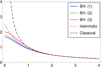
Figure 4: Plot of the Green function $G^{{L\Delta}}(R)$ for the cases (1), (2) and (3).

The divergence of the Green tensor of the bi-Helmholtz-Navier equation (48) reads

$$G_{ij,j}(\bm{R})=\frac{1-2\nu}{16\pi\mu(1-\nu)}\,\partial_{i}\Delta\,A(R)\,$$ (79)

and the double-divergence of the Green tensor of the bi-Helmholtz-Navier equation (48) reads

$$G_{ij,ij}(\bm{R})=\frac{1-2\nu}{16\pi\mu(1-\nu)}\,\Delta\Delta\,A(R)=-\frac{1-2\nu}{2\mu(1-\nu)}\,G^{\text{BH}}(R)\,.$$ (80)

2.4 Operator split in gradient elasticity

The operator split in gradient elasticity [64, 65] is mainly based on the decomposition of a partial differential equation (pde) of higher-order into a system of pdes of lower-order and on the property that the appearing differential operator(s) can be written as a product of differential operators of lower-order (operator-split). The property that the differential operators commute is also important. The problem in the theory of defects (for vanishing body forces, $\bm{b}=0$) in the framework of gradient elasticity is that both fields, the displacement field $\bm{u}$ on the left hand side and the plastic distortion $\bm{\beta}^{\text{P}}$ as source field on the right hand side of the bi-Helmholtz-Navier equation (19) are “a priori” unknown since they are both non-classical fields (see [64]).

The inhomogeneous bi-Helmholtz-Navier equation (19) for the displacement field with the plastic distortion (or eigendistortion) tensor as source field (pde of 6th-order)

$$LL_{ik}u_{k}=C_{ijkl}\partial_{j}L\beta^{{\mathrm{P}}}_{kl}\,$$ (81)

can be decomposed into the following system of partial differential equations, namely into two uncoupled inhomogeneous bi-Helmholtz equations (pdes of 4th-order)

$$Lu_{i}=u_{i}^{0}\,,$$ (82)

$$L\beta^{\mathrm{P}}_{ij}=\beta_{ij}^{{\mathrm{P}},0}\,$$ (83)

and into an inhomogeneous Navier equation (pde of 2nd-order)

$$L_{ik}u_{k}^{0}=C_{ijkl}\partial_{j}\beta^{{\mathrm{P}},0}_{kl}\,.$$ (84)

Eq. (84) is the classical Navier equation with the classical displacement vector $u_{k}^{0}$ and the classical eigendistortion tensor $\beta^{{\mathrm{P}},0}_{kl}$ known from classical eigenstrain theory, which are the source fields for Eqs. (82) and (83). Substituting Eqs. (82) and (83) into Eq. (84), Eq. (81) is recovered. Using Eq. (83), Eq. (81) gives the following bi-Helmholtz-Navier equation

$$LL_{ik}u_{k} =C_{ijkl}\partial_{j}\beta^{{\mathrm{P}},0}_{kl}\,,$$ (85)

where the right hand side is given by the gradient of the classical eigendistortion tensor. Thus, the source term in Eq. (85) is the classical source term known from Mura’s eigenstrain theory (see [54]). Eq. (85) is the basic equation in the eigenstrain formulation of gradient elasticity of bi-Helmholtz type.

If we use the Green tensor (48), then the solution of Eq. (85) is the convolution of the (negative) Green tensor with the right hand side of Eq. (85)

$$u_{i}=G_{ij}*f_{j}=-C_{jkln}G_{ij}*\beta_{ln,k}^{{\mathrm{P}},0}=-C_{jkln}G_{ij,k}*\beta_{ln}^{{\mathrm{P}},0}\,,$$ (86)

where the ficticious body force density reads as

$$f_{i}=-C_{ijkl}\partial_{j}\beta^{{\mathrm{P}},0}_{kl}\,.$$ (87)

Eq. (86) is the generalized Volterra formula for an arbitrary eigendistortion. The gradient of Eq. (86) gives the displacement gradient

$$u_{i,m}=-C_{jkln}G_{ij,km}*\beta_{ln}^{{\mathrm{P}},0}\,.$$ (88)

On the other hand, using the regularization function or mollifier of bi-Helmholtz type, $G^{\text{BH}}$, the solutions of Eqs. (82) and Eqs. (83) can be written as convolution of the classical singular solution with the mollifier

$$u_{i} =G^{\text{BH}}*u_{i}^{0}\,,$$ (89)

$$\beta^{\mathrm{P}}_{ij} =G^{\text{BH}}*\beta_{ij}^{{\mathrm{P}},0}\,.$$ (90)

3 Point defects with cubic symmetry in isotropic materials

The aim of the present section is the continuum theoretical modelling of point defects. In the theory of incompatible elasticity, point defects can be modelled as defects corresponding to a three-dimensional Dirac $\delta$-singularity in the eigendistortion tensor [10]. The eigendistortion or quasi-plastic distortion tensor of a point defect with cubic symmetry (dilatation centre) is given by

$$\beta^{{\mathrm{P}},0}_{ij}=Q_{ij}\,\delta({\bm{R}})\,\quad\text{with}\quad Q_{ij}=Q\,\delta_{ij}\,,$$ (91)

where ${\bm{R}}={\bm{x}}-{\bm{x}}^{\prime}$ and $Q$ is the strength of the cubic point defect (dilatation centre) given by

$$Q=\frac{\Delta V}{3}\,.$$ (92)

Here $\Delta V$ represents the plastic volume change [50]. The point defect, corresponding to the eigendistortion (91), is located at point ${\bm{x}}^{\prime}$. For point defects (91), the ficticious body force density (87) corresponds to double forces (see also [66])

$$f_{i}=-P_{ij}\,\partial_{j}\delta({\bm{R}})\,,\quad\text{with}\quad P_{ij}=C_{ijkl}Q_{kl}\,,$$ (93)

where $P_{ij}$ is the elastic dipole tensor or double force tensor [48, 49, 3, 10].

3.1 Point defects in gradient elasticity of bi-Helmholtz type

Now, we derive the solutions of the fields of a point defect (dilatation centre) in the framework of incompatible gradient elasticity of bi-Helmholtz type.

First, substituting

$$C_{ijkk}=2\mu\,\frac{1+\nu}{1-2\nu}\,\delta_{ij}\,$$ (94)

and (91) into Eq. (86), we obtain

$$u_{i}=-\frac{2\mu(1+\nu)Q}{(1-2\nu)}\,G_{ik,k}=-\frac{Q}{8\pi}\,\frac{1+\nu}{1-\nu}\,\partial_{i}\Delta\,A(R)\,.$$ (95)

The first gradient of Eq. (95), being the total distortion tensor, reads as

$$u_{i,j}=-\frac{2\mu(1+\nu)Q}{(1-2\nu)}\,G_{ik,kj}=-\frac{Q}{8\pi}\,\frac{1+\nu}{1-\nu}\,\partial_{j}\partial_{i}\Delta\,A(R)\,,$$ (96)

the second gradient of Eq. (95), being the first gradient of the total distortion tensor, reads as

$$u_{i,jk}=-\frac{2\mu(1+\nu)Q}{(1-2\nu)}\,G_{im,mjk}=-\frac{Q}{8\pi}\,\frac{1+\nu}{1-\nu}\,\partial_{k}\partial_{j}\partial_{i}\Delta\,A(R)\,$$ (97)

and the third gradient of Eq. (95), being the second gradient of the total distortion tensor, reads as

$$u_{i,jkl}=-\frac{2\mu(1+\nu)Q}{(1-2\nu)}\,G_{im,mjkl}=-\frac{Q}{8\pi}\,\frac{1+\nu}{1-\nu}\,\partial_{l}\partial_{k}\partial_{j}\partial_{i}\Delta\,A(R)\,.$$ (98)

Introducing the auxiliary functions, playing the mathematical role of multiplicative regularization functions,

$$f_{1}(R,c_{1},c_{2})=1 -\frac{1}{c_{1}^{2}-c_{2}^{2}}\,\Big{[}c_{1}^{2}\,{\mathrm{e}}^{-R/c_{1}}-c_{2}^{2}\,{\mathrm{e}}^{-R/c_{2}}\Big{]}-\frac{R}{c_{1}^{2}-c_{2}^{2}}\,\Big{[}c_{1}\,{\mathrm{e}}^{-R/c_{1}}-c_{2}\,{\mathrm{e}}^{-R/c_{2}}\Big{]}\,,$$ (99)

$$f_{2}(R,c_{1},c_{2})=1 -\frac{1}{c_{1}^{2}-c_{2}^{2}}\,\Big{[}c_{1}^{2}\,{\mathrm{e}}^{-R/c_{1}}-c_{2}^{2}\,{\mathrm{e}}^{-R/c_{2}}\Big{]}-\frac{R}{c_{1}^{2}-c_{2}^{2}}\,\Big{[}c_{1}\,{\mathrm{e}}^{-R/c_{1}}-c_{2}\,{\mathrm{e}}^{-R/c_{2}}\Big{]}$$

$$-\frac{R^{2}}{3(c_{1}^{2}-c_{2}^{2})}\,\Big{[}{\mathrm{e}}^{-R/c_{1}}-{\mathrm{e}}^{-R/c_{2}}\Big{]}\,,$$ (100)

$$f_{3}(R,c_{1},c_{2})=1 -\frac{1}{c_{1}^{2}-c_{2}^{2}}\,\Big{[}c_{1}^{2}\,{\mathrm{e}}^{-R/c_{1}}-c_{2}^{2}\,{\mathrm{e}}^{-R/c_{2}}\Big{]}-\frac{R}{c_{1}^{2}-c_{2}^{2}}\,\Big{[}c_{1}\,{\mathrm{e}}^{-R/c_{1}}-c_{2}\,{\mathrm{e}}^{-R/c_{2}}\Big{]}$$

$$-\frac{2R^{2}}{5(c_{1}^{2}-c_{2}^{2})}\,\Big{[}{\mathrm{e}}^{-R/c_{1}}-{\mathrm{e}}^{-R/c_{2}}\Big{]}-\frac{R^{3}}{15(c_{1}^{2}-c_{2}^{2})}\,\Big{[}\frac{1}{c_{1}}\,{\mathrm{e}}^{-R/c_{1}}-\frac{1}{c_{2}}\,{\mathrm{e}}^{-R/c_{2}}\Big{]}\,,$$ (101)

$$f_{4}(R,c_{1},c_{2})=1 -\frac{1}{c_{1}^{2}-c_{2}^{2}}\,\Big{[}c_{1}^{2}\,{\mathrm{e}}^{-R/c_{1}}-c_{2}^{2}\,{\mathrm{e}}^{-R/c_{2}}\Big{]}-\frac{R}{c_{1}^{2}-c_{2}^{2}}\,\Big{[}c_{1}\,{\mathrm{e}}^{-R/c_{1}}-c_{2}\,{\mathrm{e}}^{-R/c_{2}}\Big{]}$$

$$-\frac{3R^{2}}{7(c_{1}^{2}-c_{2}^{2})}\,\Big{[}{\mathrm{e}}^{-R/c_{1}}-{\mathrm{e}}^{-R/c_{2}}\Big{]}-\frac{2R^{3}}{21(c_{1}^{2}-c_{2}^{2})}\,\Big{[}\frac{1}{c_{1}}\,{\mathrm{e}}^{-R/c_{1}}-\frac{1}{c_{2}}\,{\mathrm{e}}^{-R/c_{2}}\Big{]}$$

$$-\frac{R^{4}}{105(c_{1}^{2}-c_{2}^{2})}\,\Big{[}\frac{1}{c^{2}_{1}}\,{\mathrm{e}}^{-R/c_{1}}-\frac{1}{c^{2}_{2}}\,{\mathrm{e}}^{-R/c_{2}}\Big{]}\,,$$ (102)

Eqs. (95)–(98) can be written as

$$u_{i} =\frac{Q}{4\pi}\frac{1+\nu}{1-\nu}\frac{R_{i}}{R^{3}}\,f_{1}(R,c_{1},c_{2})\,,$$ (103)

$$u_{i,j} =\frac{Q}{4\pi}\frac{1+\nu}{1-\nu}\bigg{[}\frac{\delta_{ij}}{R^{3}}\,f_{1}(R,c_{1},c_{2})-\frac{3R_{i}R_{j}}{R^{5}}\,f_{2}(R,c_{1},c_{2})\bigg{]}\,,$$ (104)

$$u_{i,jk} =-\frac{Q}{4\pi}\frac{1+\nu}{1-\nu}\bigg{[}\frac{3\big{(}\delta_{ij}R_{k}+\delta_{jk}R_{i}+\delta_{ki}R_{j}\big{)}}{R^{5}}\,f_{2}(R,c_{1},c_{2})-\frac{15R_{i}R_{j}R_{k}}{R^{7}}\,f_{3}(R,c_{1},c_{2})\bigg{]}\,$$ (105)

and

$$u_{i,jkl}=-\frac{Q}{4\pi}\frac{1+\nu}{1-\nu}\bigg{[}\frac{3\delta_{ijkl}}{R^{5}}\,f_{2}(R,c_{1},c_{2})$$

$$\quad-\frac{15\big{(}\delta_{ij}R_{k}R_{l}+\delta_{ik}R_{j}R_{l}+\delta_{il}R_{j}R_{k}+\delta_{jk}R_{i}R_{l}+\delta_{jl}R_{i}R_{k}+\delta_{kl}R_{i}R_{j}\big{)}}{R^{7}}\,f_{3}(R,c_{1},c_{2})$$

$$\quad+\frac{105R_{i}R_{j}R_{k}R_{l}}{R^{9}}\,f_{4}(R,c_{1},c_{2})\bigg{]}\,$$ (106)

with

$$\delta_{ijkl}=\delta_{ij}\delta_{kl}+\delta_{jk}\delta_{il}+\delta_{ik}\delta_{jl}\,.$$ (107)

In addition, the divergence of the displacement field reads as

$$u_{i,i}=\frac{Q}{4\pi}\frac{1+\nu}{1-\nu}\,\frac{3}{R^{3}}\,\big{[}f_{1}(R,c_{1},c_{2})-f_{2}(R,c_{1},c_{2})\big{]}=Q\,\frac{1+\nu}{1-\nu}\,G^{\text{BH}}(R)$$ (108)

and its first gradient is

$$u_{i,ik}=-\frac{Q}{4\pi}\frac{1+\nu}{1-\nu}\,\frac{15R_{k}}{R^{5}}\,\big{[}f_{2}(R,c_{1},c_{2})-f_{3}(R,c_{1},c_{2})\big{]}=Q\,\frac{1+\nu}{1-\nu}\,\partial_{k}G^{\text{BH}}(R)\,.$$ (109)

The auxiliary functions (73), (99)–(3.1) are plotted in Fig. 5. In the far field, the auxiliary functions (73), (99)–(3.1) approach 1 and in the near field, they are modified due to gradient parts and approach 0 at the position $R=0$ (see Fig. 5).

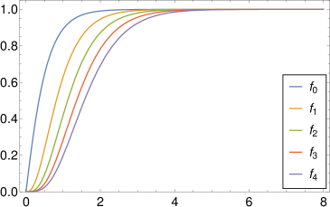
Figure 5: Plot of the auxiliary functions $f_{0}$, $f_{1}$, $f_{2}$, $f_{3}$ and $f_{4}$ for case (1).

Moreover, the quasi-plastic distortion tensor of a dilatation centre reads

$$\beta_{ij}^{\mathrm{P}}=G^{\text{BH}}(R)*\beta_{ij}^{{\mathrm{P}},0}=Q\,\delta_{ij}\,G^{\text{BH}}(R)\,,$$ (110)

the first gradient of quasi-plastic distortion tensor of a dilatation centre is

$$\beta_{ij,k}^{\mathrm{P}}=Q\,\delta_{ij}\,\partial_{k}G^{\text{BH}}(R)\,$$ (111)

and the second gradient of quasi-plastic distortion tensor of a dilatation centre reads

$$\beta_{ij,kl}^{\mathrm{P}}=Q\,\delta_{ij}\,\partial_{l}\partial_{k}G^{\text{BH}}(R)\,.$$ (112)

In Eq. (110), it can be seen that the form factor $G^{\text{BH}}$ characterizes the shape of the quasi-plastic distortion of a dilatation centre.

For a dilatation centre, the elastic strain tensor and its gradients read

$$e_{ij} =u_{i,j}-\beta_{ij}^{\mathrm{P}}\,,$$ (113)

$$e_{ij,k} =u_{i,jk}-\beta_{ij,k}^{\mathrm{P}}\,,$$ (114)

$$e_{ij,kl} =u_{i,jkl}-\beta_{ij,kl}^{\mathrm{P}}\,$$ (115)

and the elastic dilatation field and its gradients are

$$e_{ii} =-Q\,\frac{2(1-2\nu)}{1-\nu}\,G^{\text{BH}}(R)\,,$$ (116)

$$e_{ii,k} =-Q\,\frac{2(1-2\nu)}{1-\nu}\,\partial_{k}G^{\text{BH}}(R)\,,$$ (117)

$$e_{ii,kl} =-Q\,\frac{2(1-2\nu)}{1-\nu}\,\partial_{l}\partial_{k}G^{\text{BH}}(R)\,.$$ (118)

In order to study if the fields are singularity-free, the near-field behaviour of the fields (103)–(3.1) is needed. The relevant series expansion of the auxiliary functions (99)–(3.1) (near fields) reads as

$$f_{1}(R,c_{1},c_{2}) =\frac{1}{3c_{1}c_{2}(c_{1}+c_{2})}\,R^{3}-\frac{1}{8c^{2}_{1}c^{2}_{2}}\,R^{4}+\mathcal{O}(R^{5})\,,$$ (119)

$$f_{2}(R,c_{1},c_{2}) =\frac{1}{24c^{2}_{1}c^{2}_{2}}\,R^{4}+\mathcal{O}(R^{5})\,,$$ (120)

$$f_{3}(R,c_{1},c_{2}) =\frac{1}{120c^{2}_{1}c^{2}_{2}}\,R^{4}+\mathcal{O}(R^{5})\,,$$ (121)

$$f_{4}(R,c_{1},c_{2}) =\frac{1}{280c^{2}_{1}c^{2}_{2}}\,R^{4}+\mathcal{O}(R^{5})\,.$$ (122)

From Eqs. (119)–(122) it can be seen that the function $f_{1}(R,c_{1},c_{2})$ regularizes up to a $1/R^{3}$-singularity and the functions $f_{2}(R,c_{1},c_{2})$, $f_{3}(R,c_{1},c_{2})$ and $f_{4}(R,c_{1},c_{2})$ regularize up to a $1/R^{4}$-singularity and give non-singular fields.

In case (2), the auxiliary functions (99)–(3.1) become

$$f_{1}(R,c_{1},c_{1})=1 -\bigg{[}1+\frac{R}{c_{1}}+\frac{R^{2}}{2c_{1}^{2}}\bigg{]}\,{\mathrm{e}}^{-R/c_{1}}\,,$$ (123)

$$f_{2}(R,c_{1},c_{1})=1 -\bigg{[}1+\frac{R}{c_{1}}+\frac{R^{2}}{2c_{1}^{2}}+\frac{R^{3}}{6c_{1}^{3}}\bigg{]}\,{\mathrm{e}}^{-R/c_{1}}\,,$$ (124)

$$f_{3}(R,c_{1},c_{1})=1 -\bigg{[}1+\frac{R}{c_{1}}+\frac{R^{2}}{2c_{1}^{2}}+\frac{R^{3}}{6c_{1}^{3}}+\frac{R^{4}}{30c_{1}^{4}}\bigg{]}\,{\mathrm{e}}^{-R/c_{1}}\,,$$ (125)

$$f_{4}(R,c_{1},c_{1})=1 -\bigg{[}1+\frac{R}{c_{1}}+\frac{R^{2}}{2c_{1}^{2}}+\frac{R^{3}}{6c_{1}^{3}}+\frac{4R^{4}}{105c_{1}^{4}}+\frac{R^{5}}{210c_{1}^{5}}\bigg{]}\,{\mathrm{e}}^{-R/c_{1}}\,,$$ (126)

where the relevant series expansion of the auxiliary functions (123)–(126) (near fields) reads as

$$f_{1}(R,c_{1},c_{1}) =\frac{1}{6c^{3}_{1}}\,R^{3}-\frac{1}{8c^{4}_{1}}\,R^{4}+\mathcal{O}(R^{5})\,,$$ (127)

$$f_{2}(R,c_{1},c_{1}) =\frac{1}{24c^{4}_{1}}\,R^{4}+\mathcal{O}(R^{5})\,,$$ (128)

$$f_{3}(R,c_{1},c_{1}) =\frac{1}{120c^{4}_{1}}\,R^{4}+\mathcal{O}(R^{5})\,,$$ (129)

$$f_{4}(R,c_{1},c_{1}) =\frac{1}{280c^{4}_{1}}\,R^{4}+\mathcal{O}(R^{5})\,.$$ (130)

From Eqs. (127)–(130) it is obvious that the function $f_{1}(R,c_{1},c_{1})$ regularizes up to a $1/R^{3}$-singularity and the functions $f_{2}(R,c_{1},c_{1})$, $f_{3}(R,c_{1},c_{1})$ and $f_{4}(R,c_{1},c_{1})$ regularize up to a $1/R^{4}$-singularity. The auxiliary functions (75), (123)–(125) are plotted in Fig. 6.

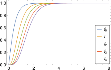
Figure 6: Plot of the auxiliary functions $f_{0}$, $f_{1}$, $f_{2}$, $f_{3}$ and $f_{4}$ for case (2).

In case (3), the auxiliary functions (99)–(3.1) reduce to

$$f_{1}(R,c_{1},c_{2})=1 -{\mathrm{e}}^{-aR}\bigg{[}\bigg{(}1+\frac{R}{2A}\bigg{)}\cos(bR)-\bigg{(}\frac{A^{2}-B^{2}}{2AB}+\frac{R}{2B}\bigg{)}\sin(bR)\bigg{]}\,,$$ (131)

$$f_{2}(R,c_{1},c_{2})=1 -{\mathrm{e}}^{-aR}\bigg{[}\bigg{(}1+\frac{R}{2A}\bigg{)}\cos(bR)-\bigg{(}\frac{A^{2}-B^{2}}{2AB}+\frac{R}{2B}+\frac{R^{2}}{6AB}\bigg{)}\sin(bR)\bigg{]}\,,$$ (132)

$$f_{3}(R,c_{1},c_{2})=1 -{\mathrm{e}}^{-aR}\bigg{[}\bigg{(}1+\frac{R}{2A}-\frac{R^{3}}{30A(A^{2}+B^{2})}\bigg{)}\cos(bR)$$

$$\qquad-\bigg{(}\frac{A^{2}-B^{2}}{2AB}+\frac{R}{2B}+\frac{R^{2}}{5AB}+\frac{R^{3}}{30B(A^{2}+B^{2})}\bigg{)}\sin(bR)\bigg{]}\,,$$ (133)

$$f_{4}(R,c_{1},c_{2})=1 -{\mathrm{e}}^{-aR}\bigg{[}\bigg{(}1+\frac{R}{2A}-\frac{R^{3}}{21A(A^{2}+B^{2})}-\frac{R^{4}}{105(A^{2}+B^{2})^{2}}\bigg{)}\cos(bR)$$

$$-\bigg{(}\frac{A^{2}-B^{2}}{2AB}+\frac{R}{2B}+\frac{3R^{2}}{14AB}+\frac{R^{3}}{21B(A^{2}+B^{2})}+\frac{R^{4}(A^{2}-B^{2})}{210AB(A^{2}+B^{2})^{2}}\bigg{)}\sin(bR)\bigg{]}$$ (134)

and the corresponding series expansion of the auxiliary functions (131)–(3.1) (near fields) reads as

$$f_{1}(R,c_{1},c_{2}) =\frac{1}{6A(A^{2}+B^{2})}\,R^{3}-\frac{1}{8(A^{2}+B^{2})^{2}}\,R^{4}+\mathcal{O}(R^{5})\,,$$ (135)

$$f_{2}(R,c_{1},c_{2}) =\frac{1}{24(A^{2}+B^{2})^{2}}\,R^{4}+\mathcal{O}(R^{5})\,,$$ (136)

$$f_{3}(R,c_{1},c_{2}) =\frac{1}{120(A^{2}+B^{2})^{2}}\,R^{4}+\mathcal{O}(R^{6})\,,$$ (137)

$$f_{4}(R,c_{1},c_{2}) =\frac{1}{280(A^{2}+B^{2})^{2}}\,R^{4}+\mathcal{O}(R^{5})\,,$$ (138)

where $A$ and $B$ are given in Eq. (38) and $a$ and $b$ are given in Eq. (40). From Eqs. (135)–(138) it can be seen that the function $f_{1}(R,c_{1},c_{2})$ regularizes up to a $1/R^{3}$-singularity and the functions $f_{2}(R,c_{1},c_{2})$, $f_{3}(R,c_{1},c_{2})$ and $f_{4}(R,c_{1},c_{2})$ regularize up to a $1/R^{4}$-singularity and give non-singular fields. The auxiliary functions (77), (131)–(3.1) are plotted in Fig. 7. It can be seen that the auxiliary functions  (77), (131)–(3.1) show a weak oscillation in the near field.

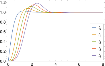
Figure 7: Plot of the auxiliary functions $f_{0}$, $f_{1}$, $f_{2}$, $f_{3}$ and $f_{4}$ for case (3).

Therefore, up to the second gradient of the displacement, the fields are non-singular. Only, the third gradient of the displacement field possesses a $1/R$-singularity. The radial part $f_{1}(R,c_{1},c_{2})/R^{2}$ of the displacement (103) is zero at $R=0$, since the near field behaves like $R$, and is plotted in Fig. 8(a). The radial parts $f_{1}(R,c_{1},c_{2})/R^{3}$ and $f_{2}(R,c_{1},c_{2})/R^{3}$ of the first displacement gradient (104) are finite and zero, respectively, at $R=0$ and are plotted in Figs. 8(b) and 8(c). The radial parts $f_{2}(R,c_{1},c_{2})/R^{4}$ and $f_{3}(R,c_{1},c_{2})/R^{4}$ of the second displacement gradient (105) are finite at $R=0$ and are plotted in Figs. 8(d) and 8(e). That means that the term $(\delta_{ij}\tau_{k}+\delta_{jk}\tau_{i}+\delta_{ki}\tau_{j})f_{2}(R,c_{1},c_{2})/R^{4}$ of the second displacement gradient (105) has a jump at $R=0$. The radial parts $f_{2}(R,c_{1},c_{2})/R^{5}$, $f_{3}(R,c_{1},c_{2})/R^{5}$ and $f_{4}(R,c_{1},c_{2})/R^{5}$ of the third displacement gradient (3.1) possess a $1/R$-singularity at $R=0$ and are plotted in Figs. 8(f), 8(g) and 8(h). The radial functions and the corresponding “classical” singularities $1/R^{2}$, $1/R^{3}$, $1/R^{4}$ and $1/R^{5}$ are plotted in Fig. 8. In Fig. 8, it can be seen that the functions $f_{1}(R,c_{1},c_{2})/R^{2}$, $f_{1}(R,c_{1},c_{2})/R^{3}$, $f_{2}(R,c_{1},c_{2})/R^{3}$, $f_{2}(R,c_{1},c_{2})/R^{4}$, $f_{3}(R,c_{1},c_{2})/R^{4}$, $f_{2}(R,c_{1},c_{2})/R^{5}$, $f_{3}(R,c_{1},c_{2})/R^{5}$ and $f_{4}(R,c_{1},c_{2})/R^{5}$ do not show weak oscillations in the near field.

Using the 3D Green function of the bi-Helmholtz equation, $G^{\text{BH}}(R)$, as regularization function with $G^{\text{BH}}(R)*1/R^{n}$, gradient elasticity of bi-Helmholtz type regularizes classical singularities up to $1/R^{4}$, namely $G^{\text{BH}}(R)*1/R^{4}$ is finite. For the order $n=5$, the classical singularity $1/R^{5}$ is regularized to a weaker singularity, namely $G^{\text{BH}}(R)*1/R^{5}\sim 1/R$.

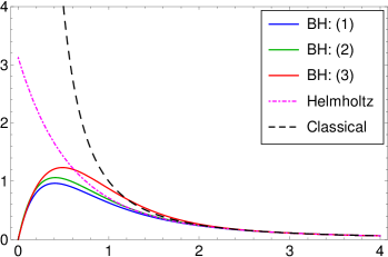
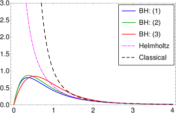
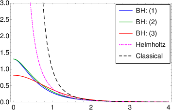
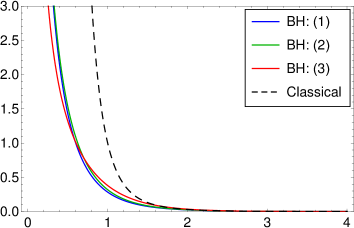
Figure 8: Plots of the radial functions in gradient elasticity of bi-Helmholtz type, gradient elasticity of Helmholtz type and classical elasticity: (a) $f_{1}/R^{2}$, (b) $f_{1}/R^{3}$, (c) $f_{2}/R^{3}$, (d) $f_{2}/R^{4}$, (e) $f_{3}/R^{4}$, (f) $f_{2}/R^{5}$, (g) $f_{3}/R^{5}$, (h) $f_{4}/R^{5}$.

Moreover, substituting Eqs. (104), (110) and (116) into Eq. (6), and using Eq. (4) and $\lambda=2\mu\nu/(1-2\nu)$, the Cauchy stress of a dilatation centre in gradient elasticity of bi-Helmholtz type is obtained as

$$\sigma_{ij} =\frac{\mu Q}{2\pi}\,\frac{1+\nu}{1-\nu}\bigg{[}\bigg{(}\frac{\delta_{ij}}{R^{3}}-\frac{3R_{i}R_{j}}{R^{5}}\bigg{)}f_{2}(R,c_{1},c_{2})-\frac{8\pi}{3}\,\delta_{ij}\,G^{\text{BH}}(R)\bigg{]}\,,$$ (139)

which is non-singular. In addition, Eq. (139) gives also the “nonlocal” stress of a dilatation centre in the framework of nonlocal elasticity of bi-Helmholtz type [41].

3.2 Limit to gradient elasticity of Helmholtz type

In the limit from gradient elasticity of bi-Helmholtz type (case (1)) to gradient elasticity of Helmholtz type (e.g. [67, 32]), $c_{2}\rightarrow 0$ and $c_{1}\rightarrow\ell$, we obtain from Eqs. (95)–(97) or Eqs. (103)–(109) the displacement field of a dilatation centre in the framework of gradient elasticity of Helmholtz type

$$u_{i}=-\frac{Q}{4\pi}\frac{1+\nu}{1-\nu}\,\partial_{i}\bigg{(}\frac{1}{R}-\frac{{\mathrm{e}}^{-R/\ell}}{R}\bigg{)}=\frac{Q}{4\pi}\frac{1+\nu}{1-\nu}\frac{R_{i}}{R^{3}}\,f_{1}(R,\ell)\,,$$ (140)

the first gradient

$$u_{i,j} =-\frac{Q}{4\pi}\frac{1+\nu}{1-\nu}\,\partial_{j}\partial_{i}\bigg{(}\frac{1}{R}-\frac{{\mathrm{e}}^{-R/\ell}}{R}\bigg{)}$$

$$=\frac{Q}{4\pi}\frac{1+\nu}{1-\nu}\bigg{[}\frac{\delta_{ij}}{R^{3}}\,f_{1}(R,\ell)-\frac{3R_{i}R_{j}}{R^{5}}\,f_{2}(R,\ell)\bigg{]}\,,$$ (141)

which can be verified by making use of the identities [68, 69]

$$\partial_{j}\partial_{i}\bigg{(}\frac{1}{R}\bigg{)} =-\frac{4\pi}{3}\,\delta_{ij}\,\delta({\bm{R}})-\frac{\delta_{ij}}{R^{3}}+\frac{3R_{i}R_{j}}{R^{5}}\,,$$ (142)

$$\partial_{j}\partial_{i}\bigg{(}\frac{\text{e}^{-R/\ell}}{R}\bigg{)} =-\frac{4\pi}{3}\,\delta_{ij}\,\delta(\bm{R})-\frac{\delta_{ij}}{R^{3}}\Big{(}1+\frac{R}{\ell}\Big{)}\text{e}^{-R/\ell}+3\frac{R_{i}R_{j}}{R^{5}}\Big{(}1+\frac{R}{\ell}+\frac{R^{2}}{3\ell^{2}}\Big{)}\text{e}^{-R/\ell}\,,$$ (143)

the second gradient

$$u_{i,jk}=-\frac{Q}{4\pi}\frac{1+\nu}{1-\nu}\bigg{[}\frac{3\big{(}\delta_{ij}R_{k}+\delta_{jk}R_{i}+\delta_{ki}R_{j}\big{)}}{R^{5}}\,f_{2}(R,\ell)-\frac{15R_{i}R_{j}R_{k}}{R^{7}}\,f_{3}(R,\ell)\bigg{]}\,$$ (144)

and the divergence of the displacement field reads

$$u_{i,i}=\frac{Q}{4\pi}\frac{1+\nu}{1-\nu}\,\frac{3}{R^{3}}\,\big{[}f_{1}(R,\ell)-f_{2}(R,\ell)\big{]}=Q\,\frac{1+\nu}{1-\nu}\,G^{\text{H}}(R)\,,$$ (145)

with the Green function of the Helmholtz operator given by

$$G^{\text{H}}(R)=\frac{1}{4\pi\ell^{2}R}\,{{\mathrm{e}}^{-R/\ell}}\,,$$ (146)

which is a Dirac-delta sequence with parametric dependence $\ell$

$$\lim_{\ell\to 0}G^{\text{H}}(R)=\delta({\bm{R}})\,.$$ (147)

Eq. (146) is the regularization function in gradient elasticity of Helmholtz type and is a “mollifier”. The quasi-plastic distortion of a dilatation centre (110) reduces to

$$\beta^{\mathrm{P}}_{ij}=Q\,\delta_{ij}\,G^{\text{H}}(R)=\frac{Q}{4\pi\ell^{2}R}\,\delta_{ij}\,{\mathrm{e}}^{-R/\ell}\,.$$ (148)

For gradient elasticity of Helmholtz type, the Green function of the Helmholtz-Laplace operator is

$$G^{L\Delta}(R)=\frac{1}{4\pi R}\,f_{0}(R,\ell)\,$$ (149)

obtained from Eqs. (72) and (73).

In the limit $c_{2}\rightarrow 0$ and $c_{1}\rightarrow\ell$, the auxiliary functions (73), (99)–(3.1) read as

$$f_{0}(R,\ell) =1-{\mathrm{e}}^{-R/\ell}\,,$$ (150)

$$f_{1}(R,\ell) =1-\bigg{[}1+\frac{R}{\ell}\bigg{]}\,{\mathrm{e}}^{-R/\ell}\,,$$ (151)

$$f_{2}(R,\ell) =1-\bigg{[}1+\frac{R}{\ell}+\frac{1}{3}\,\frac{R^{2}}{\ell^{2}}\bigg{]}\,{\mathrm{e}}^{-R/\ell}\,,$$ (152)

$$f_{3}(R,\ell) =1-\bigg{[}1+\frac{R}{\ell}+\frac{2}{5}\,\frac{R^{2}}{\ell^{2}}+\frac{1}{15}\,\frac{R^{3}}{\ell^{3}}\bigg{]}\,{\mathrm{e}}^{-R/\ell}\,.$$ (153)

The auxiliary functions (150)–(153) are plotted in Fig. 9 for $\ell=0.4a_{0}$. For gradient elasticity of Helmholtz type, the near field behaviour of the fields (140)–(144) is needed. The relevant series expansion of the auxiliary functions (151)–(153) (near fields) reads as

$$f_{0}(R,\ell) =\frac{1}{\ell}\,R-\frac{1}{2\ell^{2}}\,R^{2}+\mathcal{O}(R^{3})\,,$$ (154)

$$f_{1}(R,\ell) =\frac{1}{2\ell^{2}}\,R^{2}-\frac{1}{3\ell^{3}}\,R^{3}+\frac{1}{8\ell^{4}}\,R^{4}+\mathcal{O}(R^{5})\,,$$ (155)

$$f_{2}(R,\ell) =\frac{1}{6\ell^{2}}\,R^{2}-\frac{1}{24\ell^{4}}\,R^{4}+\mathcal{O}(R^{5})\,,$$ (156)

$$f_{3}(R,\ell) =\frac{1}{10\ell^{2}}\,R^{2}-\frac{1}{120\ell^{4}}\,R^{4}+\mathcal{O}(R^{5})\,.$$ (157)

From Eq. (154) it is obvious that the function $f_{0}(R,\ell)$ regularizes up to a $1/R$-singularity and gives a non-singular field expression. From Eqs. (155)–(157) it can be seen that the functions $f_{1}(R,\ell)$, $f_{2}(R,\ell)$ and $f_{3}(R,\ell)$ regularize up to a $1/R^{2}$-singularity and give non-singular fields. At $R=0$ the auxiliary functions (150)–(153) are zero and in the far field they approach 1.

Thus, the displacement field is non-singular and finite at $R=0$, but suffers a jump due to $\tau_{i}f_{1}(R,\ell)/R^{2}$. The first displacement gradient possesses a $1/R$-singularity, and the second displacement gradient possesses a $1/R^{2}$-singularity (see Fig. 8).

Using the 3D Green function of the Helmholtz equation, $G^{\text{H}}(R)$, with $G^{\text{H}}(R)*1/R^{n}$, gradient elasticity of Helmholtz type regularizes singularities up to $1/R^{2}$, namely $G^{\text{BH}}(R)*1/R^{2}$ is finite. For the order $n=3$, $G^{\text{BH}}(R)*1/R^{3}\sim 1/R$, and for the order $n=4$, $G^{\text{BH}}(R)*1/R^{4}\sim 1/R^{2}$.

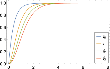
Figure 9: Plot of the auxiliary functions $f_{0}$, $f_{1}$, $f_{2}$ and $f_{3}$ in gradient elasticity of Helmholtz type.

Moreover, it is interesting to notice that Eqs. (140)–(144) agree with the expressions given in [22].

3.3 Limit to classical elasticity

The limit from gradient elasticity of Helmholtz type to classical elasticity is $\ell\rightarrow 0$ and we obtain from Eqs. (140) and (3.2) the classical displacement field of a dilatation centre

$$u^{0}_{i}=-\frac{Q}{4\pi}\frac{1+\nu}{1-\nu}\,\partial_{i}\bigg{(}\frac{1}{R}\bigg{)}=\frac{Q}{4\pi}\frac{1+\nu}{1-\nu}\,\frac{R_{i}}{R^{3}}\,$$ (158)

and its gradient, being the total distortion tensor,

$$u^{0}_{i,j} =-\frac{Q}{4\pi}\frac{1+\nu}{1-\nu}\,\partial_{j}\partial_{i}\bigg{(}\frac{1}{R}\bigg{)}$$

$$=\frac{Q}{4\pi}\frac{1+\nu}{1-\nu}\bigg{[}\frac{\delta_{ij}}{R^{3}}\,-\frac{3R_{i}R_{j}}{R^{5}}+\frac{4\pi}{3}\,\delta_{ij}\,\delta({\bm{R}})\bigg{]}\,.$$ (159)

The total dilatation, which follows from Eq. (3.3),

$$u^{0}_{i,i}=Q\,\frac{1+\nu}{1-\nu}\,\delta(\bm{R})$$ (160)

and the quasi-plastic dilatation of a dilatation centre

$$\beta^{{\mathrm{P}},0}_{ij}=Q\,\delta_{ij}\delta({\bm{R}})$$ (161)

are given in terms of a Dirac delta function. The displacement field possesses a $1/R$-singularity, and the displacement gradient possesses a $1/R^{2}$-singularity and a $\delta({\bm{R}})$-singularity. Note that the Dirac delta term in the total distortion (3.3) is often erroneously neglected (see, e.g., [2]).

4 Interaction energy and interaction force between defects in gradient elasticity of bi-Helmholtz type

In this Section, we investigate the interaction between two dilatation centres as well as a dilatation centre with an edge dislocation in the framework of gradient elasticity of bi-Helmholtz type. We consider case (1) as characteristic example. As we have shown in Section 3, cases (2) and (3) have a similar behaviour as case (1) and can be easily obtained from case (1).

4.1 Interaction energy

In gradient elasticity of bi-Helmholtz type, the interaction energy is given by

$$U_{\text{int}}=\int_{V}\big{(}\sigma_{ij}e_{ij}+\tau_{ijk}\partial_{k}e_{ij}+\tau_{ijkl}\partial_{l}\partial_{k}e_{ij}\big{)}\,{\mathrm{d}}V=\int_{V}L\sigma_{ij}e_{ij}\,{\mathrm{d}}V=-\int_{V}\sigma_{ij}\beta^{{\mathrm{P}},0}_{ij}\,{\mathrm{d}}V\,,$$ (162)

where we have used integration by parts, the Green-Gauss theorem with vanishing surface terms at infinity and Eqs. (1) and (83).

4.1.1 Interaction energy between two point defects

Substituting Eq. (91) into Eq. (162), the interaction energy between a point defect with $Q_{ij}$ in the stress field $\sigma_{ij}$ of another defect, or with $P_{ij}$ in the elastic strain field $e_{ij}$, reads (see, e.g., [10])

$$U_{\text{int}}=-Q_{ij}\sigma_{ij}=-P_{ij}e_{ij}\,.$$ (163)

For a dilatation centre, the interaction energy (163) reduces to

$$U_{\text{int}}=-Q\sigma_{ii}=-Pe_{ii}\,.$$ (164)

Substituting Eqs. (116) and (173) into (164), the interaction energy becomes

$$U_{\text{int}}=QQ^{\prime}\,4\mu\,\frac{1+\nu}{1-\nu}\,G^{\text{BH}}(R)\,.$$ (165)

Using the Green function (54), the interaction energy (164) between the two dilatational centres reduces to

$$U_{\text{int}}=\frac{QQ^{\prime}\mu(1+\nu)}{\pi(1-\nu)}\,\frac{1}{(c_{1}^{2}-c_{2}^{2})}\,\frac{1}{R}\Big{(}{\mathrm{e}}^{-R/c_{1}}-{\mathrm{e}}^{-R/c_{2}}\Big{)}\,.$$ (166)

In Fig. 3(a), it can be seen that the interaction energy (165) is a short-range interaction energy and remains finite if $R\rightarrow 0$. For $QQ^{\prime}<0$, the interaction energy (166) possesses a minimum at $R=0$, and for $QQ^{\prime}>0$, the interaction energy (166) possesses a maximum at $R=0$. In fact, using gradient elasticity of bi-Helmholtz type, the finite short-range interaction energy is the regularization of the contact term in the interaction energy discussed in [10]:

$$\lim_{c_{1}\to 0,\,c_{2}\to 0}U_{\text{int}}=QQ^{\prime}\,4\mu\,\frac{1+\nu}{1-\nu}\,\delta({\bm{R}})\,.$$ (167)

In the limit to gradient elasticity of Helmholtz type, $c_{1}\rightarrow\ell$ and $c_{2}\rightarrow 0$, the interaction energy (166) reduces to

$$U_{\text{int}}=\frac{QQ^{\prime}\mu(1+\nu)}{\pi(1-\nu)\ell^{2}}\,\,\frac{{\mathrm{e}}^{-R/\ell}}{R}\,,$$ (168)

which has the form of a Yukawa potential known from the physics of nucleons [70, 71]. For $R\rightarrow 0$, the Yukawa potential has a $1/R$-singularity. Therefore, the non-singular interaction energy (166) between two dilatation centres may be called bi-Yukawa potential.

4.1.2 Self-energy of a dilatation centre

Using Eq. (55), Eq. (165) delivers the finite self-energy of a dilatation centre with $Q=Q^{\prime}$

$$U_{\text{s}}=\frac{1}{2}\,U_{\text{int}}(0)=\frac{Q^{2}}{2\pi}\,\mu\,\frac{1+\nu}{1-\nu}\,\frac{1}{c_{1}c_{2}(c_{1}+c_{2})}\,.$$ (169)

Eq. (169) means that the self-energy of a point defect is equivalent to half the interaction energy between two identical point defects when $R=0$. The finite Green function (form factor) (54) has assured a finite self-energy.

4.2 Interaction force

The interaction force can be written as (negative) gradient of the interaction energy (see also [10])

$${\cal{F}}_{k}=-\partial_{k}U_{\text{int}}\,.$$ (170)

4.2.1 Interaction force between two point defects

Using the interaction energy (163), we obtain from Eq. (170) the force exerted on the point defect in the gradient of a stress field or in the gradient of an elastic strain field

$${\cal{F}}_{k}=Q_{ij}\sigma_{ij,k}=P_{ij}e_{ij,k}\,.$$ (171)

Eq. (171) gives the interaction force between a point defect of strength $Q_{ij}$ and the stress gradient field $\sigma_{ij,k}$, which can be caused by other defects (point defect, dislocation). On the other hand, the material force (171) can be expressed in terms of the elastic dipole tensor $P_{ij}$ and the elastic strain gradient tensor (see also [48, 45, 10]). For a dilatation centre, the interaction force (171) simplifies to

$${\cal{F}}_{k}=Q\sigma_{ii,k}=Pe_{ii,k}\,,$$ (172)

where

$$P=2\mu\,\frac{1+\nu}{1-2\nu}\,Q\,.$$ (173)

Using Eqs. (116) and (173), we obtain from Eq. (172)

$${\cal{F}}_{k}=-QQ^{\prime}\,4\mu\,\frac{1+\nu}{1-\nu}\,\partial_{k}G^{\text{BH}}(R)\,.$$ (174)

Substituting Eq. (61) into (174), the interaction force between two dilatation centres reads as

$${\cal{F}}_{k}=\frac{QQ^{\prime}\mu\,(1+\nu)}{\pi(1-\nu)}\,\frac{1}{(c_{1}^{2}-c_{2}^{2})}\,\frac{R_{k}}{R^{3}}\bigg{[}{\mathrm{e}}^{-R/c_{1}}-{\mathrm{e}}^{-R/c_{2}}+\frac{R}{c_{1}}\,{\mathrm{e}}^{-R/c_{1}}-\frac{R}{c_{2}}\,{\mathrm{e}}^{-R/c_{2}}\bigg{]}\,.$$ (175)

Therefore, the interaction force (175) between two dilatation centres is a short-range interaction force. The force (175) is the short-range interaction force exerted by one point defect with strength $Q^{\prime}$ at ${\bm{x}}^{\prime}$ on the other point defect with strength $Q$ at ${\bm{x}}$. Here, $R$ is the distance between the two defects from $Q^{\prime}$ to $Q$, and ${\bm{R}}={\bm{x}}-{\bm{x}}^{\prime}$ is the vector from $Q^{\prime}$ to $Q$. Using Eq. (62), it can be seen that Eq. (174) is finite at $R=0$

$${\cal{F}}_{k}(0)=\frac{QQ^{\prime}}{2\pi}\,\mu\,\frac{1+\nu}{1-\nu}\,\frac{1}{c_{1}^{2}c_{2}^{2}}\,\tau_{k}\,.$$ (176)

In the limit to gradient elasticity of Helmholtz type, $c_{1}\rightarrow\ell$ and $c_{2}\rightarrow 0$, the interaction force (175) reduces to a singular Yukawa type force

$${\cal{F}}_{k}=\frac{QQ^{\prime}\mu\,(1+\nu)}{\pi(1-\nu)\ell^{2}}\,\frac{R_{k}}{R^{3}}\bigg{(}1+\frac{R}{\ell}\bigg{)}\,{\mathrm{e}}^{-R/\ell}\,.$$ (177)

Therefore, the non-singular interaction force (175) between two dilatation centres is a bi-Yukawa type force.

4.3 Interaction between an edge dislocation and a dilatation centre

The aim of this subsection is to study the interaction between an edge dislocation and a point defect (dilatation centre) which is of importance for the understanding of the properties of solids. We consider a point defect in the stress field of an edge dislocation.

The hydrostatic stress field of an edge dislocation with (positive) Burgers vector $b_{x}$ located at $(x,y)=(0,0)$ in the framework of gradient elasticity of bi-Helmholtz type is given by [31]

$$\sigma_{ii}=-\frac{\mu b_{x}(1+\nu)}{\pi(1-\nu)}\,\frac{\sin\varphi}{r}\Big{\{}1-\frac{1}{c_{1}^{2}-c_{2}^{2}}\big{[}c_{1}rK_{1}(r/c_{1})-c_{2}rK_{1}(r/c_{2})\big{]}\Big{\}}\,,$$ (178)

where $r=\sqrt{x^{2}+y^{2}}$.

4.3.1 Interaction energy

If Eq. (178) is substituted into (164), the interaction energy between an edge dislocation and a dilatation centre is obtained as

$$U_{\text{int}}=\frac{\mu Qb_{x}(1+\nu)}{\pi(1-\nu)}\,\frac{\sin\varphi}{r}\Big{\{}1-\frac{1}{c_{1}^{2}-c_{2}^{2}}\big{[}c_{1}rK_{1}(r/c_{1})-c_{2}rK_{1}(r/c_{2})\big{]}\Big{\}}\,.$$ (179)

The point defect is located at $(r,\varphi)$. For an oversized point defect ($Q>0$), $U_{\text{int}}$ is positive for positions above the slip plane ($0<\varphi<\pi$) and negative below ($\pi<\varphi<2\pi$) since the edge dislocation produces compression in the region of the extra half-plane and tension below. For an undersized point defect ($Q<0$) the positions of attraction and repulsion are reversed. An important feature of this result is that, contrary to the classical result, the interaction energy remains finite if $r\rightarrow 0$ as it can be seen in Fig. 10. The minimum of the interaction energy near the dislocation line at $\varphi=\pi/4$ gives the binding energy between an edge dislocation and a vacancy (negative dilatation centre) or undersized poind defect ($Q<0$) and at $\varphi=3\pi/4$ gives the binding energy between an edge dislocation and an oversized point defect (positive dilatation centre) ($Q>0$). The position and the value of the binding energy depend on the lengths $c_{1}$ and $c_{2}$. If $c_{2}\rightarrow 0$ and $c_{1}\rightarrow 0$, then the classical Cottrell-Bilby result is recovered [72].

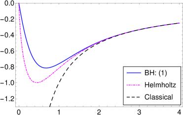
Figure 10: Interaction energy between a point defect and an edge dislocation in gradient elasticity of bi-Helmholtz type, gradient elasticity of Helmholtz type and classical elasticity for $\varphi=3\pi/4$ in units of $\mu Qb_{x}(1+\nu)/[\pi(1-\nu)a_{0}]$.

In the limit to gradient elasticity of Helmholtz type, $c_{1}\rightarrow\ell$ and $c_{2}\rightarrow 0$, the interaction energy (179) reduces to

$$U_{\text{int}}=\frac{\mu Qb_{x}(1+\nu)}{\pi(1-\nu)}\,\frac{\sin\varphi}{r}\Big{\{}1-\frac{r}{\ell}\,K_{1}(r/\ell)\Big{\}}\,,$$ (180)

which is still singularity-free (see Fig. 10). For $Q>0$ at $\varphi=3\pi/4$, the interaction energy (180) has minimum of $U_{\text{int}}=0.399\mu Qb_{x}(1+\nu)/[\pi(1-\nu)\ell]$ at $r=1.114\ell$. Using the value of $\ell=0.49a_{0}$ for Al ($a_{0}=4.05$ Å) calculated in the framework of gradient elasticity of Helmholtz type [56, 55], the position of the minimum of the interaction energy (binding energy) is $U_{\text{int}}=0.814\mu Qb_{x}(1+\nu)/[\pi(1-\nu)a]$ at $r=0.546a_{0}=0.772b_{x}$ where $b_{x}=a_{0}/\sqrt{2}$ is the Burgers vector in fcc. Moreover, it is interesting to notice that Eq. (180) is in agreement with the expression given in [23].

4.3.2 Interaction force

The interaction force between an edge dislocation and a dilatation centre is given by

$${\cal{F}}_{r} =-\frac{\partial U_{\text{int}}}{\partial r}$$

$$=\frac{\mu Qb_{x}(1+\nu)}{\pi(1-\nu)}\,\frac{\sin\varphi}{r^{2}}\Big{\{}1-\frac{1}{c_{1}^{2}-c_{2}^{2}}\big{[}c_{1}rK_{1}(r/c_{1})-c_{2}rK_{1}(r/c_{2})\big{]}$$

$$\hskip 142.26378pt-\frac{r^{2}}{c_{1}^{2}-c_{2}^{2}}\big{[}K_{0}(r/c_{1})-K_{0}(r/c_{2})\big{]}\Big{\}}$$ (181)

and

$${\cal{F}}_{\varphi} =-\frac{1}{r}\,\frac{\partial U_{\text{int}}}{\partial\varphi}$$

$$=-\frac{\mu Qb_{x}(1+\nu)}{\pi(1-\nu)}\,\frac{\cos\varphi}{r^{2}}\Big{\{}1-\frac{1}{c_{1}^{2}-c_{2}^{2}}\big{[}c_{1}rK_{1}(r/c_{1})-c_{2}rK_{1}(r/c_{2})\big{]}\Big{\}}\,.$$ (182)

Both components ${\cal{F}}_{r}$ and ${\cal{F}}_{\varphi}$ are plotted in Fig. 11 and it can be seen that they are finite at $r=0$. Figure 11 shows the interaction force as a function of the distance between the edge dislocation and the point defect. It can be seen in Fig. 11(a) that near the edge dislocation a bound state appears when ${\cal{F}}_{r}=0$ (position of minimum of $U_{\text{int}}$). The position at ${\cal{F}}_{r}=0$ is the equilibrium position of the point defect in the stress field of an edge dislocation not present in classical elasticity. We notice a significant deviation between the classical results and the gradient results in Figs. 10 and 11 when the defect separation is less than $r=2a_{0}$ because classical elasticity is not valid at such a scale unlike gradient elasticity. In particular, ${\cal{F}}_{r}$ changes the sign near the dislocation unlike the classical result (see Fig. 11(a)).

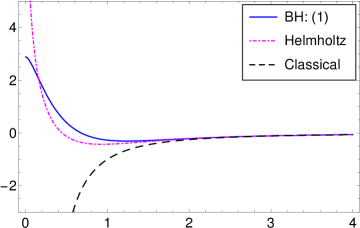
Figure 11: Interaction force between a point defect and an edge dislocation in gradient elasticity of bi-Helmholtz type, gradient elasticity of Helmholtz type and classical elasticity: (a) ${\cal{F}}_{r}$, (b) ${\cal{F}}_{\varphi}$, for $\varphi=3\pi/4$ in units of $\mu Qb_{x}(1+\nu)/[\pi(1-\nu)a_{0}^{2}]$.

In the limit to gradient elasticity of Helmholtz type, $c_{1}\rightarrow\ell$ and $c_{2}\rightarrow 0$, the interaction force between an edge dislocation and a dilatation centre, Eqs. (4.3.2) and (4.3.2), reduces to

$${\cal{F}}_{r} =\frac{\mu Qb_{x}(1+\nu)}{\pi(1-\nu)}\,\frac{\sin\varphi}{r^{2}}\Big{\{}1-\frac{r}{\ell}\,K_{1}(r/\ell)-\frac{r^{2}}{\ell^{2}}\,K_{0}(r/\ell)\Big{\}}$$ (183)

and

$${\cal{F}}_{\varphi} =-\frac{\mu Qb_{x}(1+\nu)}{\pi(1-\nu)}\,\frac{\cos\varphi}{r^{2}}\Big{\{}1-\frac{r}{\ell}\,K_{1}(r/\ell)\Big{\}}\,.$$ (184)

${\cal{F}}_{r}=0$ at $r=1.114\ell$. Eqs. (183) and (184) possess a $\ln r$-singularity at $r=0$. Using the value of $\ell=0.49a_{0}$ for Al calculated in the framework of gradient elasticity of Helmholtz type [56, 55], the equilibrium position of the point defect in the stress field of an edge dislocation reads: $r=0.546a_{0}$. For Aluminum, it reads: $r=2.211\,\text{\AA}$. Note that Eq. (183) is in agreement with the expression given in [23].

5 Conclusion

In this paper, we have presented and developed a non-singular continuum theory of point defects. It is based on a second strain gradient elasticity theory, the so-called gradient elasticity of bi-Helmholtz type, with eigenstrain caused by point defects. We discussed possible values for the two characteristic internal lengths of gradient elasticity of bi-Helmholtz type ($\ell_{1}$, $\ell_{2}$), which are two material parameters describing the range of the weak nonlocality present near the defects. Our model is able to give non-singular expressions for the displacement field, the first displacement gradient, the second displacement gradient, the plastic distortion and the first gradient of the plastic distortion. This fact makes it possible to solve a set of problems unsolvable in classical elasticity as well as in gradient elasticity of Helmholtz type. Unlike the singular expression in classical elasticity and in gradient elasticity of Helmholtz type, we have found non-singular and finite expressions for:

• interaction energy between two dilatation centres (bi-Yukawa potential)

• interaction force between two dilatation centres (bi-Yukawa force)

• self-energy of a dilatation centre

• interaction force between a dilatation centre and an edge dislocation .

Moreover, unlike the singular expression in classical elasticity, we have found

• interaction energy between a dilatation centre and an edge dislocation

similar to the non-singular expression obtained in gradient elasticity of Helmholtz type leading to realistic expressions of binding energies and of the equilibrium position of a point defect in the stress field of an edge dislocation. The obtained fields of point defects are non-singular due to a straightforward and self-consistent regularization based on the bi-Helmholtz operator and Green function. The non-singular fields are important and necessary for a better discrete dislocation dynamics and computer simulations of non-singular defects. Moreover, all the obtained non-singular analytical expressions can be compared with corresponding atomistic and experimental results.

For the three-dimensional solutions (e.g. Green functions, displacement and displacement gradients) in gradient elasticity of bi-Helmholtz type, there are three types of solutions:

• in case (1), the solutions are given in terms of two decreasing exponential functions $\exp(-r/c_{1})$ and $\exp(-r/c_{2})$

• in case (2), the solutions are given in terms of one decreasing exponential function $\exp(-r/c_{1})$

• in case (3), the solutions are given in terms of one decreasing exponential function $\exp(-ar)$ times sine and/or cosine functions: $\sin(br)$ and $\cos(br)$.

Although the auxiliary lengths $c_{1}$ and $c_{2}$ can be real or complex conjugate, the material lengths $\ell_{1}$ and $\ell_{2}$ are always real. In other words, independent if the auxiliary lengths $c_{1}$ and $c_{2}$ are real or complex conjugate, the physical behaviour of the displacement and displacement gradients of a dilatation centre is not changed and it does not show oscillations. Therefore, the physical behaviour of the displacement and displacement gradients of a dilatation centre in the possible cases (1), (2) and (3) is similar.

References

- Leibfried and Breuer [1978] G. Leibfried and N. Breuer, Point Defects in Metals I, Springer Tracts in Modern Physics, Vol. 81 (Springer, Berlin, 1978).
- Teodosiu [1982] C. Teodosiu, Elastic Models of Crystal Defects, (Springer, Berlin, 1982).
- Balluffi [2012] R.W. Balluffi, Introduction to Elasticity Theory for Crystal Defects (Cambridge University Press, Cambridge, 2012).
- Nabarro [1967] F.R.N. Nabarro, Theory of Crystal Dislocations, (Oxford University Press, Oxford, 1967).
- Clouet [2006] E. Clouet, The vacancy-edge dislocation interaction in fcc metals: A comparison between atomic simulations and elasticity theory, Acta Materialia 54 (2006), 3543–3552.
- Varvenne et al. [2013] C. Varvenne, F. Bruneval, M.C. Marinica, and E. Clouet, Point defect modeling in materials: coupling ab initio and elasticity approaches, Physical Review B 88 (2013), 134102.
- Clouet et al. [2018] E. Clouet, C. Varvenne, and T. Jourdan, Elastic modeling of point-defects and their interaction, Computational Materials Science 147 (2018), 49–63.
- Eshelby [1955] J.D. Eshelby, The elastic interaction of point defects, Acta Metallurgica 3 (1955), 487–490.
- Eshelby [1956] J.D. Eshelby, The continuum theory of lattice defects, Solid State Physics 3 (1956), 79–144.
- Lazar [2017] M. Lazar, Micromechanics and theory of point defects in anisotropic elasticity, Journal of Micromechanics and Molecular Physics 2 (2017), 1750005 [19 pages].
- Eringen [2002] A.C. Eringen, Nonlocal Continuum Field Theories, (Springer, New York, 2002).
- Kovács [1981] I. Kovács, Nonlocal elastic interaction between point defects and dislocations, Archive of Mechanics 33 (1981), 901–908.
- Wang [1990] R. Wang, Non-local elastic interaction energy between a dislocation and a point defect, Journal of Physics D: Applied Physics 23 (1990), 263–265.
- Polvstenko [2001] Yu.Z. Povstenko, Point defects in a nonlocal elastic medium, Journal of Mathematical Sciences 104 (2001), 1501–1505.
- Gairola [1976] B.K.D. Gairola, The nonlocal theory of elastic and its application to interaction between point defects, Archives of Mechanics 28 (1976), 393–404.
- Gairola [1978] B.K.D. Gairola, Nonlocal theory of elastic interaction between point defects, Physica Status Solidi (b) 85 (1978), 577–585.
- Vörös and Kovács [1993] G. Vörös and I. Kovács, Static lattice defects in a quasi-continuum, physica status solidi (b) 178 (1993), 99–107.
- Vörös and Kovács [1995] G. Vörös and I. Kovács, Elastic interaction between point defects and dislocations in quasi-continuum, Philosophical Magazine A 72 (1995), 949–961.
- Adler [1969] W.F. Adler, Point-defect interactions in elastic materials of grade 2, Physical Review 186 (1969), 666–674.
- Toupin [1962] R.A. Toupin, Elastic materials with couple-stresses, Archive of Rational Mechanics and Analysis 11 (1962), 385–414.
- Mindlin [1964] R.D. Mindlin, Micro-structure in linear elasticity, Archive of Rational Mechanics and Analysis 16 (1964), 51–78.
- Dobovšeck [2006] I. Dobovšek, Problem of a point defect, spatial regularization and intrinsic length scale in second gradient elasticity, Materials Science and Engineering A 423 (2006), 92–96.
- Vlasov [2001] N.M. Vlasov, Interaction of point defects with an edge dislocation in the gradient theory of elasticity, Physics of the Solid State 43 (2001), 2083–2086.
- Wang et al. [2016] Z. Wang, S. Rudraraju, and K. Garikipati, A three dimensional field formulation, and isogeometric solutions to point and line defects using Toupin’s theory of gradient elasticity at finite strains, Journal of the Mechanics and Physics of Solids 94 (2016), 336–361.
- Mindlin [1965] R.D. Mindlin, Second gradient of strain and surface-tension in linear elasticity, International Journal of Solids and Structures 1 (1965), 417–438.
- Mindlin [1972] R.D. Mindlin, Elasticity, piezoelectricity and crystal lattice dynamics, Journal of Elasticity 2 (1972), 217–282.
- Jaunzemis [1967] W. Jaunzemis, Continuum Mechanics, (The Macmillan Company, New York, 1967).
- Wu [1992] C.H. Wu, Cohesive elasticity and surface phenomena, Quarterly of Applied Mathematics L 1 (1992), 73–103.
- Agiasofitou and Lazar [2009] E.K. Agiasofitou and M. Lazar, Conservation and balance laws in linear elasticity of grade three, Journal of Elasticity 94 (2009), 69–85.
- Truskinovsky and Vainchtein [2005] L. Truskinovsky and A. Vainchtein, Quasicontinuum modelling of short-wave instabilities in crystal lattices, Philosophical Magazine 85 (2005), 4055–4065.
- Lazar et al. [2006] M. Lazar, G.A. Maugin, and E.C. Aifantis, Dislocations in second strain gradient elasticity, International Journal of Solids and Structures 43 (2006), 1787–1817; Addendum, International Journal of Solids and Structures 47 (2010), 738–739.
- Lazar and Maugin [2005] M. Lazar and G.A. Maugin, Nonsingular stress and strain fields of dislocations and disclinations in first strain gradient elasticity, International Journal of Engineering Science 43 (2005), 1157–1184.
- Polizzotto [2003] C. Polizzotto, Gradient elasticity and nonstandard boundary conditions, International Journal of Solids and Structures 40 (2003), 7399–7423.
- Zhang et al. [2006] X. Zhang, K. Jiao, P. Sharma, and B.I. Yakobson, An atomistic and non-classical continuum field theoretic perspective of elastic interactions between defects (force dipoles) of various symmetries and application to graphene, Journal of the Mechanics and Physics of Solids 54 (2006), 2304–2329.
- Lazar and Maugin [2006] M. Lazar and G.A. Maugin, Dislocations in gradient elasticity revisited, Proceedings of the Royal Society A 462 (2006), 3465–3480.
- Lazar [2013] M. Lazar, The fundamentals of non-singular dislocations in the theory of gradient elasticity: Dislocation loops and straight dislocations, International Journal of Solids and Structures 50 (2013), 352–362.
- Deng et al. [2007] S. Deng, J. Liu, and N. Liang, Wedge and twist disclinations in second strain gradient elasticity, International Journal of Solids and Structures 44 (2007), 3646–3665.
- Mousavi [2016] S.M. Mousavi, Dislocation-based fracture mechanics within nonlocal and gradient elasticity of bi-Helmholtz type-Part I: Antiplane analysis, International Journal of Solids and Structures 87 (2016), 222–235.
- Mousavi [2016] S.M. Mousavi, Dislocation-based fracture mechanics within nonlocal and gradient elasticity of bi-Helmholtz type-Part II: Inplane analysis, International Journal of Solids and Structures 92-93 (2016), 105–120.
- Lyu and Li [2019] D. Lyu and S. Li, A multiscale dislocation pattern dynamics: Towards an atomistic-informed crystal plasticity theory, Journal of the Mechanics and Physics of Solids 122 (2019), 613–632.
- Lazar et al. [2006] M. Lazar, G.A. Maugin, and E.C. Aifantis, On the theory of nonlocal elasticity of bi-Helmholtz type and some applications, International Journal of Solids and Structures 43 (2006), 1404–1421.
- Fafalias et al. [2012] D.A. Fafalis, S.P. Filopoulos, and G.J. Tsamasphyros, On the capability of generalized continuum theories to capture dispersion characteristics at the atomic scale, European Journal of Mechanics-A/Solids 36 (2012), 25–37.
- Cordero et al. [2016] N.M. Cordero, S. Forest, and E.P. Busso, Second strain gradient elasticity of nano-objects, Journal of the Mechanics and Physics of Solids 97 (2016), 92–124.
- Khakalo and Niiranen [2018] S. Khakalo and J. Niiranen, Form II of Mindlin’s second strain gradient theory of elasticity with a simplification: For materials and structures from nano- to macro-scales, European Journal of Mechanics-A/Solids 71 (2018), 292–319.
- Kröner [1960] E. Kröner, Allgemeine Kontinuumstheorie der Versetzungen und Eigenspannungen, Archive of Rational Mechanics and Analysis 4 (1960), 273–333.
- deWit [1981] R. deWit, A view of the relation between the continuum theory of lattice defects and non-Euclidean geometry in the linear approximation, International Journal of Engineering Science 19 (1981), 1475–1506.
- Kröner [1956] E. Kröner, Die Versetzung als elementare Eigenspannungsquelle, Zeitschrift für Naturforschung A 11 (1956), 969–985.
- Kröner [1958] E. Kröner, Kontinuumstheorie der Versetzungen und Eigenspannungen, (Springer, Berlin, 1958).
- Kröner [1981] E. Kröner, Continuum Theory of Defects, in: Physics of Defects (Les Houches, Session 35), Balian R. et al., eds., pp. 215–315, (North-Holland, Amsterdam, 1981).
- deWit [1973] R. deWit, Theory of disclinations III, Journal of Research of the National Bureau of Standards 77A (1973), 359–368.
- Polizzotto [2016] C. Polizzotto, A note on the higher order strain and stress tensors within deformation gradient elasticity theories: Physical interpretations and comparisons, International Journal of Solids and Structures 90 (2016), 116–121.
- Forest and Sab [2012] S. Forest and K. Sab, Stress gradient continuum theory, Mechanics Research Communications 40 (2012), 16–25.
- Polizzotto [2018] C. Polizzotto, A micromorphic approach to stress gradient elasticity theory with an assessment of the boundary conditions and size effects, Z. Angew. Math. Mech. 98 (2018), 1528–1553.
- Mura [1987] T. Mura, Micromechanics of Defects in Solids, 2nd edition, (Martinus Nijhoff, Dordrecht, 1987).
- Shodja et al. [2013] H.M. Shodja, A. Zaheri, and A. Tehranchi, Ab initio calculations of characteristic lengths of crystalline materials in first strain gradient elasticity, Mechanics of Materials 61 (2013), 73–78.
- Lazar [2017] M. Lazar, Non-singular dislocation continuum theories: Strain gradient elasticity versus Peierls-Nabarro model, Philosophical Magazine 97 (2017), 3246–3275.
- Po et al. [2018] G. Po, M. Lazar, N.C. Admal, and N. Ghoniem, A non-singular theory of dislocations in anisotropic crystals, International Journal of Plasticity 103 (2018), 1–22.
- Shodja et al. [2012] H.M. Shodja, F. Ahmadpoor, and A. Tehranchi, Calculation of the additional constants for fcc materials in second strain gradient elasticity: Behavior of a nano-size Bernoulli-Euler beam with surface effects, Journal of Applied Mechanics 79 (2012), 021008 (8 pages).
- Ojaghnezhad and Shodja [2013] F. Ojaghnezhad and H.M. Shodja, A combined first principles and analytical determination of the modulus of cohesion, surface energy, and the additional constants in the second strain gradient elasticity, International Journal of Solids and Structures 50 (2013), 3967–3974.
- Eringen [1983] A.C. Eringen, On differential equations of nonlocal elasticity and solutions of screw dislocation and surface waves, Journal of Applied Physics 54 (1983), 4703–4710.
- Kunin [1983] I.A. Kunin, Elastic Media with Microstructure II: Three-Dimensional Models, (Springer, Berlin, 1983).
- Giusti [1984] E. Giusti, Minimal surfaces and functions of bounded variations, (Birkhäuser, Basel-Boston-Stuttgart, 1984).
- Bacon et al. [1979] D.J. Bacon, D.M. Barnett, and R.O. Scattergood, Anisotropic continuum theory of defects, Progress in Materials Science 23 (1979), 51–262.
- Lazar [2014] M. Lazar, On gradient field theories: gradient magnetostatics and gradient elasticity, Philosophical Magazine 94 (2014), 2840–2874.
- Ru and Aifantis [1993] C.Q. Ru and E.C. Aifantis, A simple approach to solve boundary-value problems in gradient elasticity, Acta Mechanica 101 (1993), 59–68.
- Kossecka [1971] E. Kossecka, Surface distribution of double forces, Archive of Mechanis 23 (1971), 313–328.
- Altan and Aifantis [1997] B.C. Altan and E.C. Aifantis, On some aspects in the special theory of gradient elasticity, Journal of the Mechanical Behavior of Materials 8 (1997), 231–282.
- Rogula [1973] D. Rogula, Some basic solutions in strain gradient elasticity theory of an arbitrary order, Archives of Mechanics 25 (1973), 43–68.
- Frahm [1983] C.P. Frahm, Some novel delta-function identities, American Journal of Physics 51 (1983), 826–829.
- Wentzel [1949] G. Wentzel, Quantum Theories of Fields, (Interscience Publishers, New York, 1949).
- Felsager [1998] B. Felsager, Geometry, Particles, and Fields, (Springer, New York, 1998).
- Cottrell and Bilby [1949] A.H. Cottrell and B.A. Bilby, Dislocation theory of yielding and strain ageing of iron, Proceedings of the Physical Society A 62 (1949), 49–62.