A Bayesian Poisson-Gaussian Process Model for Popularity Learning in Edge-Caching Networks

Abstract

Edge-caching is recognized as an efficient technique for future cellular networks to improve network capacity and user-perceived quality of experience. To enhance the performance of caching systems, designing an accurate content request prediction algorithm plays an important role. In this paper, we develop a flexible model, a Poisson regressor based on a Gaussian process, for the content request distribution. The first important advantage of the proposed model is that it encourages the already existing or seen contents with similar features to be correlated in the feature space and therefore it acts as a regularizer for the estimation. Second, it allows to predict the popularities of newly-added or unseen contents whose statistical data is not available in advance. In order to learn the model parameters, which yield the Poisson arrival rates or alternatively the content popularities, we invoke the Bayesian approach which is robust against over-fitting. However, the resulting posterior distribution is analytically intractable to compute. To tackle this, we apply a Markov Chain Monte Carlo (MCMC) method to approximate this distribution which is also asymptotically exact. Nevertheless, the MCMC is computationally demanding especially when the number of contents is large. Thus, we employ the Variational Bayes (VB) method as an alternative low complexity solution. More specifically, the VB method addresses the approximation of the posterior distribution through an optimization problem. Subsequently, we present a fast block-coordinate descent algorithm to solve this optimization problem. Finally, extensive simulation results both on synthetic and real-world datasets are provided to show the accuracy of our prediction algorithm and the cache hit ratio (CHR) gain compared to existing methods from the literature.

I Introduction

Recently, there has been a tremendous growth in mobile data traffic due to the increasing number of mobile devices and growing user interest towards bandwidth-hungry applications (e.g., 4K videos). According to a recent Cisco report [1], it is predicted that from 2016 to 2021 mobile traffic will increase at a $47\%$ compound annual growth rate (CAGR), two times faster than the growth of global IP fixed traffic during the same period. Nevertheless, such an inevitable growth has raised concerns about the flow of wireless traffic that traditional network architectures can tolerate. To cope with this, much effort has have been devoted towards designing and developing the 5th generation (5G) wireless cellular systems. The 5G system must provide fast, flexible, reliable and continuous wireless connectivity, while supporting the growing mobile traffic.

In this respect, caching popular contents at the network edge has been introduced  [2, 3] as an efficient solution to tackle the aforementioned issues. By observing that only a small number of popular contents are frequently requested by users, bringing these contents from the core network closer to the end mobile users avoids downloading the same content multiple times through the backhaul links. As a result, by serving users locally, edge-caching can jointly increase connectivity, reduce the delay, alleviate the backhaul link congestion and improve quality of service (QoS) of mobile users.

There has been a growing research interest in edge-caching networks, the majority of which has focused on the development and the performance analysis of various cache placement and delivery strategies taking into account that popularities are perfectly known. For example, in [2] a cache placement algorithm has been proposed to minimize the expected downloading time for contents. In a multiple base station scenario, the authors of [4] studied a probabilistic caching policy to increase content diversity in the caches. In [5], physical layer features are used in the cache placement problem to minimize network cost while satisfying users’ QoS requirements. The authors in [6] investigated energy efficiency and delivery time of an edge-caching network. In addition, various coding schemes, intra and inter sessions, have been proposed to enhance caching performance [2, 7, 8].

Still, the performance of caching schemes in the first place depends on popularity estimation accuracy. Therefore, understanding content popularity is of great importance. In real life, there are various factors that influence the way users consume contents such as social interactions, culture, user profiles, content features and so on. Nevertheless, all the underlying factors that affect users to consume contents might be either difficult to model or unavailable at the edge network (e.g. due to privacy issues). Hence, discovering the hidden content request pattern is a challenging task. Another important issue is that content producers constantly introduce new contents to the system. Proactively caching these contents can benefit both users and content providers. However, statistical data for these new or unseen contents is rarely available which makes proactive caching difficult.

I-A Related Work

During the recent years, several papers investigated machine learning techniques to predict the content popularity. In this context, the popularity learning problem can be categorized in two general approaches: model-free and model-based. In the model-free approach, there is no assumption on the content request distribution. The popularity learning is then performed within the process of optimizing a reward function (e.g cache hit ratio) by the so-called exploration-exploitation procedure. Multi-armed-bandit (MAB) and reinforcement learning algorithms are mostly based on this approach which also have been adapted to edge-caching applications [9, 10, 11, 12]. On the other hand, in the model-based approach, it is assumed that the content requests are generated by a parametric distribution. The Poisson stochastic process is a popular model adopted in content delivery networks [13] and has also been used in edge-caching [14, 15]. Once the request generation process is modeled, the next step is to estimate the popularity. A simple way is to take the average of the instantaneous requests, which is equivalent to the maximum likelihood estimation (MLE) from the estimation theory perspective. MLE performs well when the size of request samples is large. However, as it is reported in [16], a base station cache typically may receive 0.1 requests/content/day which is too small in comparison with a typical content delivery network cache which normally receives 50 requests/content/day. This indicates that MLE provides inaccurate estimation of content popularity in the local caches.

To improve the popularity estimation accuracy, side information (user profile and content features) can also be incorporated in learning algorithms. In [17, 14], users’ social interactions are leveraged to speed up the learning convergence rate. One important issue with this kind of side information is that users may not be willing to share their personal profiles with the entity operating the edge caches. On the other hand, content features (e.g topic categories) can easily and cheaply be obtained from the content server without jeopardizing users’ privacy. In [18], the authors used the content features to predict the popularity of unseen contents. More recently, the content features are used to learn the user-level preferences [19]. However, due to the data scarcity issue in the local caches, the estimation is prone to overfitting and may not be accurate. Most importantly though, it is widely admitted that in order to have accurate prediction, a more complex model is needed. This will help the network operator to identify underlying hidden structures of the content request generative process, discover popular but unseen contents and disseminate them optimally in order to improve the content delivery in the network.

I-B Contributions

In this paper, we take content features into account and introduce a new sophisticated probabilistic model for the content requests. The learning process is performed in the Bayesian paradigm which is robust against overfitting and provides a way to quantify our uncertainty about the estimation. The model allows us to define different types of predictive distributions by which we can effectively model the uncertainty of future requests. The statistical information of these posterior predictive distributions can potentially be used to enhance the performance of a caching policy. Overall, the main contributions of the paper are summarized as:

• We provide a probabilistic model for stationary content requests which exploits the similarities between contents. This model can perform two important tasks. First, it encourages the seen contents with similar features to have close popularities. In other words, it acts as a regularizer and as a result it provides a better estimation accuracy. Therefore, our model is much more flexible for popularity prediction than the method proposed in [18] where features are used only to predict the popularity of unseen content. Second, similar to [18] but in a more efficient way, our model can predict the popularity of unseen contents where statistical information is not available in advance.

• We introduce a Poisson regressor based on a Gaussian process to model the content requests. The Gaussian process is a very flexible nonparametric statistical structure that can model complex nonlinear relationships between the popularities and the features. In addition, a Bayesian method is developed to learn the parameters of the proposed probabilistic model. Due to few content request samples in the local cache, Bayesian learning provides a powerful framework to mitigate overfitting.

• Since there is no closed form solution for the posterior distribution, two inference algorithms are presented. First, the HMC method is used to estimate the posterior distribution which asymptotically provides an exact solution. Because the HMC can be computationally demanding, we introduce the VB method which turns the inference problem into an optimization. To efficiently solve this, an algorithm based on a combination of coordinate descent and parallel computing is developed.

This paper is organized as follows. The system model and problem statement are described in Section II. In Section III, our probabilistic model is introduced. In Section IV, we apply the Bayesian approach where two methods, namely the HMC and the VB, are presented for the inference task. Finally, Section V shows the simulation results and Section VI concludes the paper.

Notation: lower- (upper-) case boldface letters denote column vectors (matrices), whose ($i$,$j$)-th entry is represented by ${\left[.\right]_{ij}}$. ${\left(.\right)^{-1}}$ and ${\left(.\right)^{T}}$ denote inverse and transpose, respectively.

Figure 1: The system model of a cache-enabled cellular network

II System Model and problem formulation

In this paper, we consider a cache-enabled cellular network consisting of a base station (BS) which serves mobile users within its coverage area as shown in Fig.1. There are $U$ mobile users in the cell, where each user makes random requests from a library of contents ${\cal C}=\left\{{{c_{1}},...,{c_{M}}}\right\}$, where $M$ is the total number of contents.

The BS is equipped with a cache which can store a certain number of contents depending on its storage capacity. Moreover, the BS is connected to a remote content server which has access to the whole content library ${\cal C}$ through the backhaul links. Time is divided into different time slots and at each time slot, each user independently requests a content (or contents) from the library ${\cal C}$. To alleviate the traffic burden on the backhaul links and increase the users’ QoS, some contents are stored in the cache depending on the caching policy. The requested contents by the users will be served directly if they are already cached; otherwise they are fetched from the content server. We suppose that the cache module of the BS can only monitor the number of user requests towards contents of the library and cannot or is not allowed to perform any user profiling. In addition, it is assumed that the content popularity is fixed (we can assume it does not considerably change over short time intervals, e.g. a few days or weeks) and the requests are samples generated from a stationary distribution.

We define ${{\bf{d}}_{c}}\left[{{T_{n}}}\right]=\left[{{d_{{c_{1}}}}\left[{{T_{n}}}\right],...,{d_{{c_{M}}}}\left[{{T_{n}}}\right]}\right]^{T}$ to be the request vector where $d_{{c_{m}}}\left[{{T_{n}}}\right]$ is the total number of requests for content $m$ during time slot $n$ with duration $T_{n}$. For simplicity, we assume that $T_{n}=T_{n^{\prime}}$ $\forall n^{\prime}\neq n$ . Therefore, we can drop $T$ and show the request vector by ${{\bf{d}}_{c,n}}=\left[{{d_{{c_{1}},n}},...,{d_{{c_{M}},n}}}\right]^{T}$. Also, the requests for $n^{\prime}\neq n$ are presumed to be statistically independent random variables. A common parametric model for the requests is the Poison stochastic process i.e. ${{\bf{d}}_{c,n}}\sim Poi\left({\bf{r}}\right),\forall n=1,2,...$, where ${\bf{r}}$ is the Poisson arrival rate or the content popularity. Here, we should also mention that the Zipf distribution, which is widely used in the literature (e.g. [20]), is not a distribution to model the requests. Specifically, it only models the ordered means of requests not the requests themselves.

Any caching algorithm needs an estimate of content popularities ${\bf{r}}=E\left\{{{{\bf{d}}_{c}}}\right\}$ to operate. For example, a common caching strategy is to maximize the average CHR:

$$\mathop{\max}\limits_{\bf{w}}\,{{\bf{w}}^{T}}{\bf r}$$ (1a)

$$s.t:{{\bf{w}}^{T}}{\bf{s}}\leq C$$ (1b)

$${\bf{w}}\in{\left\{{0,1}\right\}^{M\times 1}}$$ (1c)

where $C$ is the cache size and $\bf w$ is the cache design variable.

A simple way to approximate the popularity of a content is the average number of requests within $N$ observation time slots:

$${r_{m}}\approx\frac{{\sum\limits_{n=1}^{N}{{d_{{c_{m}},n}}}}}{N},\quad\forall m=1,...,M$$ (2)

Eq. (2) is equivalent to the MLE approach for popularity estimation which is very simple, but it has some flaws. First, it suffers from severe overfitting especially when the training set has only a few request observations. Second, it cannot incorporate any kind of side information. For example, users commonly request contents based on their features and therefore we expect content popularities to be correlated in their feature space. By appropriately using this underlying prior knowledge about requests, popularity estimation precision can be significantly improved. Learning the correlation in the content feature space can also help to predict the popularity of an unseen content.

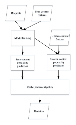
Figure 2: Illustration of content popularity learning and caching

To overcome these issues, we adopt the Bayesian modeling scheme. In this approach, both data, $\bf d$, and parameters, $\bf r$, are considered to be random variables and the first step is to define a joint distribution over them:

$$p\left({{\bf{d}},{\bf{r}}}\right)=\underbrace{p\left({{\bf{d}}|{\bf{r}}}\right)}_{\begin{array}[]{*{20}{c}}{{\rm{data}}\,\,\,\,\,{\rm{generative}}}\\ {{\mkern 1.0mu}{\kern 1.0pt}{\mkern 1.0mu}{\kern 1.0pt}{\mkern 1.0mu}{\kern 1.0pt}{\mkern 1.0mu}{\kern 1.0pt}{\mkern 1.0mu}{\kern 1.0pt}{\mkern 1.0mu}{\kern 1.0pt}{\mkern 1.0mu}{\kern 1.0pt}{\mkern 1.0mu}{\kern 1.0pt}{\mkern 1.0mu}{\kern 1.0pt}{\mkern 1.0mu}{\kern 1.0pt}{\mkern 1.0mu}{\kern 1.0pt}{\rm{pdf}}}\end{array}}\underbrace{p\left({{\bf{r}};{\boldsymbol{\zeta}}}\right)}_{\begin{array}[]{*{20}{c}}{{\rm{prior}}}\\ {{\mkern 1.0mu}{\kern 1.0pt}{\rm{pdf}}}\end{array}}$$ (3)

where the data generative distribution models the way data is generated given the parameters and the prior distribution represents the initial uncertainty of the parameters. The prior distribution may also have some parameters, $\boldsymbol{\zeta}$, which are called the hyper-parameters and usually assumed deterministic.

Fig. 2 presents our work-flow scheme for popularity learning and caching. In the model learning block, the proposed probabilistic model is trained based on the requests and the features of seen contents. In the popularity predicting blocks, the popularities of both seen and unseen content are predicted. Finally, a decision about which content should be cached is taken in the cache placement policy block.

III The content request model

In this section, we present our Bayesian probabilistic model. Before introducing the model, we summarize the basic concepts of Gaussian processes which are essential for the subsequent sections.

III-A Gaussian Processes in a Nutshell

Gaussian processes are powerful non-parametric Bayesian tools suitable for modeling real-world problems. A Gaussian process is a collection of random variables, any finite number of which have a joint Gaussian distribution. Using a Gaussian process, we can define a distribution over non-parametric functions $f\left({\bf{x}}\right)$:

$$f\left({\bf{x}}\right)\sim{\cal G}{\cal P}\left({{{\mu}}\left({\bf{x}}\right),{{K}}\left({{\bf{x}},{\bf{x^{\prime}}}}\right)}\right)$$ (4)

where $\bf x$ is an arbitrary input variable with $Q$ dimensions, and the mean function, ${{{\mu}}\left({\bf{x}}\right)}$, and the Kernel function, $K\left({{\bf{x}},{\bf{x^{\prime}}}}\right)$, are respectively defined as:

$${\bf{\mu}}\left({\bf{x}}\right)=E\left[{f\left({\bf{x}}\right)}\right]$$ (5)

$$K\left({{\bf{x}},{\bf{x^{\prime}}}}\right)=E\left[{\left({f\left({\bf{x}}\right)-\mu\left({\bf{x}}\right)}\right)\left({f\left({{\bf{x^{\prime}}}}\right)-\mu\left({{\bf{x^{\prime}}}}\right)}\right)}\right].$$ (6)

This means that a collection of $M$ function value samples has a joint Gaussian distribution:

$$\left[{f\left({{{\bf{x}}_{1}}}\right),...,f\left({{{\bf{x}}_{M}}}\right)}\right]^{T}\sim{\cal N}\left({{\boldsymbol{\mu}},{\bf{K}}}\right)$$ (7)

where ${\boldsymbol{\mu}}={\left[{\mu\left({{{\bf{x}}_{1}}}\right),...,\mu\left({{{\bf{x}}_{M}}}\right)}\right]^{T}}$ and the covariance matrix ${\bf K}$ has entries ${\left[{\bf{K}}\right]_{i,j}}=K\left({{{\bf{x}}_{i}},{{\bf{x}}_{j}}}\right)$. The kernel function specifies the main characteristics of the function that we wish to model and the basic assumption is that variables $\bf x$ which are close are likely to be correlated. Constructing a good kernel function for a learning task depends on intuition and experience. In this paper, we only focus on a popular and simple kernel which is the squared exponential kernel (SEK). However, our methodology can easily be applied to other types of Kernels. The SEK has the following form:

$$K\left({{{\bf{x}}_{i}},{{\bf{x}}_{j}}}\right)={\alpha_{0}}{e^{-\sum\limits_{q=1}^{Q}{{\alpha_{q}}{{\left\|{{x_{q,i}}-{x_{q,j}}}\right\|}^{2}}}}}$$ (8)

where ${\alpha_{0}}$ is the vertical scale variation and ${\alpha_{q}}$ is the horizontal scale variation on dimension $q$ of the function. By using different scales for each input dimension, we vary their importance. If ${\alpha_{q}}$ is close to zero, dimension $q$ will have little influence on the covariance of function values. The covariance function (8) is infinitely differentiable and is thus very smooth. More details about Gaussian processes and kernel functions can be found in [21].

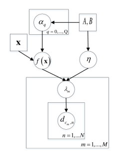
Figure 3: The proposed probabilistic model for content requests

III-B The proposed probabilistic model

In this subsection, we introduce our probabilistic model for content requests. Each content is assumed to have a set of features. For instance, YouTube videos may belong to specific categories (e.g education, art, entertainment, science-technology,.. ) and have some other features such as release year, language and so on. We let ${{\bf{x}}_{m}}$ be the feature vector of content $c_{m}$ with $Q$ dimensions whose values can be either binary or continuous. The proposed regression-based hierarchical (multilevel) probabilistic model is the following:

$${d_{{c_{m}},n}}|{\lambda_{m}}\left({{{\bf{x}}_{m}}}\right)\sim Poi\left({{e^{{\lambda_{m}}\left({{{\bf{x}}_{m}}}\right)}}}\right),\forall n=1,...,N$$ (9a)

$${\lambda_{m}}\left({{{\bf{x}}_{m}}}\right)|f\left({{{\bf{x}}_{m}}}\right),{\eta}\sim{\cal N}\left({f\left({{{\bf{x}}_{m}}}\right),{\eta}}\right)$$ (9b)

$$f\left({\bf{x}}\right)|{\bf{x}},{\alpha_{0}},...,{\alpha_{Q}}\sim{\cal GP}\left({0,K\left({{\bf{x}},{\bf{x^{\prime}}}}\right)}\right)$$ (9c)

$$\eta,{\alpha_{0}},...,{\alpha_{Q}}\sim Gam\left({A,B}\right).$$ (9d)

The first level of the model, (9a), is the observation distribution for content requests. At this level, the request for content $c_{m}$ is assumed to follow a Poisson distribution with natural parameter ${\lambda_{m}}\left({{{\bf{x}}_{m}}}\right)$ which is a function of its features. We note here that the request rate is an exponential function of the natural parameter, ${r_{m}}\left({{{\bf{x}}_{m}}}\right)={e^{{\lambda_{m}}\left({{{\bf{x}}_{m}}}\right)}}$. As we previously mentioned, it is expected that there is a similar request pattern between contents with similar features. This prior information is employed at the higher levels. In (9b), ${\lambda_{m}}\left({{{\bf{x}}_{m}}}\right)$ follows a normal distribution with mean $f\left({{{\bf{x}}_{m}}}\right)$ and variance ${\eta}$. By this assumption, we allow contents with exactly the same features to have different popularities which is possible in practice. At the higher level of the model, (9c), we assume that $\left\{{f\left({{{\bf{x}}_{m}}}\right)}\right\}_{m=1}^{M}$ are realizations of function $f\left({\bf{x}}\right)$ drawn from a Gaussian process with zero mean and kernel function $K$. By this assumption, contents with similar features are encouraged to be correlated in the feature space. Finally, in level (9d), we introduce uncertainty in the values of ${\boldsymbol{{{\theta}}}}={[\eta,{\alpha_{0}},...,{\alpha_{Q}}]^{T}}$ since in practice the available prior knowledge may not be enough to fix them. Therefore, we use a Gamma distribution, $Gam\left({A,B}\right)$, as a prior for them where $A$ and $B$ are respectively the shape and scale parameters. The corresponding graphical model of (9) is depicted in Fig. 3. The plates represent multiple samples of random variables. The unshaded circle nodes indicate unknown quantities and the squares show the deterministic parameters of the model.

We should mention that the line separating the priors and the generative distribution in model (9) depends on the question in hand. More specifically, the generative distribution for content requests is Poisson in (9a) while the other distributions consist the prior for the natural parameter of the Poisson. On the other hand, the generative distribution for the popularities is a Gaussian process in (9b) and (9c), while (9d) is the prior for the parameters of the Gaussian process. This separation lets us define two predictive distributions: for the seen contents and the unseen ones. This part is further explained in Section IV-B.

The proposed model is very flexible and can be easily extended. For example, it can be developed to model the content requests on user-level. Assume that for user $u$ in the cell there is vector ${\bf p}_{u}$ with dimensions $P$ which contains his profile information. The following probabilistic model can be used as a generative distribution for one user’s requests:

$${d_{{c_{m}},u,n}}|{\lambda_{m,u}}\left({{{\bf{x}}_{m}},{{\bf{p}}_{u}}}\right)\!\sim\!Poi({{e^{{\lambda_{m}}\left({{{\bf{x}}_{m}},{{\bf{p}}_{u}}}\right)}}}),\forall n=1,...,N$$ (10a)

$${\lambda_{m}}\left({{{\bf{x}}_{m}},{{\bf{p}}_{u}}}\right)|f\left({{{\bf{x}}_{m}},{{\bf{p}}_{u}}}\right),{\eta_{u}}\sim{\cal N}\left({f\left({{{\bf{x}}_{m}},{{\bf{p}}_{u}}}\right),{\eta_{u}}}\right)$$ (10b)

$$f\left({{{\bf{x}}},{{\bf{p}}}}\right)|{\bf{x}},{\bf{p}}\sim{\cal{GP}}\left({0,K\left({{{\bf{x}}},{{\bf{p}}},{{\bf{x}^{\prime}}},{{\bf{p}^{\prime}}}}\right)}\right).$$ (10c)

with the new kernel function defined as:

$$K\left({{{\bf{x}}_{m}},{{\bf{p}}_{u}},{{\bf{x}}_{m^{\prime}}},{{\bf{p}}_{u^{\prime}}}}\right)=$$

$${\alpha_{0,u}}{e^{-\sum\limits_{p=1}^{P}{{\beta_{pu}}{{\left\|{{p_{p,u}}-{p_{p,u^{\prime}}}}\right\|}^{2}}}-\sum\limits_{q=1}^{Q}{{\alpha_{qu}}{{\left\|{{x_{q,m}}-{x_{q,m^{\prime}}}}\right\|}^{2}}}}}.$$ (11)

Similarly to (9), we can use Gamma distributions to model the uncertainty in the parameters of the kernel function. The model in (10) allows the popularities to be correlated in the joint space of user and content features. Because, in practice, users may have different tastes (like or dislike) about the content features, we let the kernel parameters be different for each user in the content feature space.

However, there is a major issue that may discourage us to use model (10). Due to privacy concerns, user profiles may not be available at the BS and therefore from now on we only focus on the cell-level content request model (9). In the next section, we show how to learn this model and make predictions based on it.

IV Model Learning

In this section, we utilize the Bayesian framework to learn the probabilistic model in (9). In other words, given the content request observations ${\cal D}=\left\{{{{\bf{d}}_{c,n}}}\right\}_{n=1}^{N}$, we aim to update our uncertainty about the model’s parameters, $\left\{{{\lambda_{m}}\left({{{\bf{x}}_{m}}}\right)}\right\}_{m=1}^{M},f\left({\bf{x}}\right),{{\boldsymbol{\theta}}}$. However, we cannot estimate the infinite-dimensional function $f\left({\bf{x}}\right)$ and hence the focus is only on the realizations $\left\{{f\left({{{\bf{x}}_{m}}}\right)}\right\}_{m=1}^{M}$. Moreover, to simplify the inference, we can integrate out ${f\left({{{\bf{x}}_{m}}}\right)}$ from the model. By doing this, we have:

$${\boldsymbol{\lambda}}={\left[{{\lambda_{1}}\left({{{\bf{x}}_{1}}}\right),....,{\lambda_{M}}\left({{{\bf{x}}_{M}}}\right)}\right]^{T}}\sim{\cal N}\left({{\bf{0}},{\bf{\tilde{K}}}}\right)$$ (12)

where ${\bf{\tilde{K}}}={\bf{K}}+{\eta}{\bf{I}}$.

The inference of all unknown parameters of the model is given by the Bayes rule as:

$$p\left({{\boldsymbol{\lambda}},{\boldsymbol{\theta}}|{\cal D}}\right)=\frac{{p\left({{\cal D}|{\boldsymbol{\lambda}}}\right)\,p\left({{\boldsymbol{\lambda}}|{\boldsymbol{\theta}}}\right)\prod\limits_{q=0}^{Q+1}{p\left({{\theta_{q}}}\right)}}}{Z}$$ (13)

where $p\left({{\cal D}|{\boldsymbol{\lambda}}}\right)=\prod\limits_{n=1}^{N}{\prod\limits_{m=1}^{M}{p\left({{d_{{c_{m}},n}}|{\lambda_{m}}}\right)}}$ , $p\left({{\boldsymbol{\lambda}},{{\boldsymbol{\theta}}}|{\cal D}}\right)$ is the posterior distribution and the denominator $Z$ is a normalization constant also called the marginal likelihood. Nevertheless, the normalization constant is intractable to compute and additionally there is no closed-form expression for the posterior distribution. So, instead, we use a Markov Chain Monte Carlo (MCMC) method to approximate the posterior distribution. The goal of MCMC methods is to generate a set of independent samples from the target posterior distribution with enough samples to perform accurate inferences. Specifically, here, we use the Hamiltonian Monte Carlo (HMC) method which has been one of the most successful HMC methods to sample from an unnormalized distribution. Next, we give a brief overview of the HMC whose complete description can be found in [22].

HMC is based on the simulation of Hamiltonian dynamics as a method to generate a sequence of samples $\left\{{{{\boldsymbol{\zeta}}^{\left(s\right)}}}\right\}_{s=1}^{S}$ from a desired $D$-variate distribution $p\left({\boldsymbol{\zeta}}\right)$ by exploring its sample space. It combines gradient information of $p\left({\boldsymbol{\zeta}}\right)$ and auxiliary variables, ${\bf p}\in R^{D\times 1}$, with density $p\left({\bf{p}}\right)={\cal N}\left({{\bf{0}},{\bf{G}}}\right)$. The Hamiltonian function is then defined as:

$$H\left({{\boldsymbol{\zeta}},{\bf{p}}}\right)=\psi\left({\boldsymbol{\zeta}}\right)+\frac{1}{2}\log{\left({2\pi}\right)^{D}}{\bf{G}}+\frac{1}{2}{{\bf{p}}^{T}}{\bf{G}}{\bf{p}}$$ (14)

where $\psi\left(\boldsymbol{\zeta}\right)$ is the negative log of the unnormalized $p\left(\boldsymbol{\zeta}\right)$ and ${\bf{G}}$ is usually assumed to be the identity matrix. The physical analogy of (14) is a system with Hamiltonian dynamics which describe the total energy of the system as the sum of the potential energy (the first term) and the kinetic energy (the last two terms). Moreover, HMC is only applicable for differentiable and unconstrained variables. However, in (13), there are some variables, ${{\boldsymbol{\theta}}}$, that must be positive. To handle this issue, we exploit the exponential-transformation where instead of $\theta_{q}$, we use ${\phi_{q}}=\log(\theta_{q})$ with ${{\phi_{q}}}$ serving as an unconstrained auxiliary variable. Note that to use these transformations, we also need to compute the Jacobian determinant as a result of the change of random variables.

By defining ${\boldsymbol{\zeta}}\!\!=\!\!{\left[{{{\boldsymbol{\lambda}}^{T}},{\phi_{0}},...{\phi_{Q+1}}}\right]^{T}}\!\!\in{R^{(M+Q+2)\times 1}}$ and $p\left(\boldsymbol{\zeta}\right)$ as the posterior distribution (13), the negative log of the unnormalized $p\left(\boldsymbol{\zeta}\right)$ (after the exponential-transformation) is given by:

$$\psi\left(\boldsymbol{\zeta}\right)=-\log p\left({{\boldsymbol{\lambda}},{\boldsymbol{\theta}}|{\cal D}}\right)\!\!=\!\!\sum\limits_{m=1}^{M}{\sum\limits_{n=1}^{N}{-{d_{c_{m}n}}{\lambda_{m}}}}+{e^{{\lambda_{m}}}}$$

$$+\frac{1}{2}\log\det\left({{\bf{\tilde{K}}}}\right)+\frac{1}{2}{{\boldsymbol{\lambda}}^{T}}{{{\bf{\tilde{K}}}}^{-1}}{\boldsymbol{\lambda}}+\sum\limits_{q=0}^{Q+1}{-{A_{q}}{\phi_{q}}+{B_{q}}{e^{{\phi_{q}}}}}.$$ (15)

Also, the gradient of (IV) can be easily computed by using matrix derivatives [23]:

$$\begin{array}[]{*{20}{l}}{\frac{{\psi\left({\boldsymbol{\zeta}}\right)}}{{\partial{\lambda_{m}}}}=\sum\limits_{n=1}^{N}{-{d_{c_{m}n}}}+N{e^{{\lambda_{m}}}}\!+\!\!{{\left[{{{{\bf{\tilde{K}}}}^{-1}}{\boldsymbol{\lambda}}}\right]}_{m}}}\\ {\frac{{\psi\left({\boldsymbol{\zeta}}\right)}}{{\partial{\phi_{q}}}}\!=\!\frac{1}{2}tr\left({{{{\bf{\tilde{K}}}}^{-1}}\frac{{\partial{\bf{\tilde{K}}}}}{{\partial{\phi_{q}}}}}\right)\!-\!\frac{1}{2}{{\boldsymbol{\lambda}}^{T}}{{{\bf{\tilde{K}}}}^{-1}}\frac{{\partial{\bf{\tilde{K}}}}}{{\partial{\phi_{q}}}}{{{\bf{\tilde{K}}}}^{-1}}{\boldsymbol{\lambda}}\!\!-\!\!{A_{q}}+{B_{q}}{e^{{\phi_{q}}}}}.\end{array}$$

1

Input: $\boldsymbol{\zeta}^{0}$

Output: $\left\{{{{\boldsymbol{\zeta}}^{\left(s\right)}}}\right\}_{s=1}^{S}$

/* draw $S$ samples from $p\left(\zeta\right)$ */

2 Set ${{\bf{\zeta}}^{\left(1\right)}}={{\bf{\zeta}}^{0}}$;

3 for $s\leftarrow 1$ to $S$ do

4      

5      ${\bf q}^{(1)}={\boldsymbol{\zeta}}^{(s)}$, ${\bf{p}}^{(1)}\sim{\cal N}\left({{\bf{0}},{\bf{G}}}\right)$;

6       Compute $H\left({{{\bf{q}}^{(1)}},{{\bf{p}}^{(1)}}}\right)$;

7       for $l\leftarrow 1$ to $L$ do

8             ${\bf{p}}={{\bf{p}}^{(l)}}-\varepsilon\nabla\psi\left({{{\bf{q}}^{(l)}}}\right)$;

9            

10            ${\boldsymbol{q}}^{(l+1)}={\boldsymbol{q}}^{(l)}+\varepsilon{{\bf{G}}^{-1}}{\bf{p}}$;

11             ${{\bf{p}}^{(l+1)}}={\bf{p}}-\varepsilon\nabla\psi\left({{{\bf{q}}^{(l+1)}}}\right)$;

12            

13       end for

14      compute $dH=H\left({\boldsymbol{q}^{(L+1)},{\bf p}^{(L+1)}}\right)-H\left({\boldsymbol{q}^{(1)},{\bf{p}}^{(1)}}\right)$;

15       if $rand\left({}\right)<{e^{-dH}}$ then

             $\boldsymbol{\zeta}^{s+1}={\boldsymbol{q}}^{(L+1)}$;

              /* accept */

16            

17      else

             $\boldsymbol{\zeta}^{s+1}={\boldsymbol{q}}^{(1)}$;

              /* reject */

18            

19       end if

20      

21 end for

Algorithm 1 The HMC sampling algorithm

The HMC sampling is depicted in Alg.1. Lines $5$ to $9$ represent the discretized version of the continuous Hamiltonian equations called the leapfrog method which has $2$ parameters, the number of steps $L$ and the stepsize $\epsilon$. In lines $10-15$, the new sample proposed by the Hamiltonian dynamics simulation is evaluated. If it decreases the total system energy in (14) it gets accepted as a new sample, otherwise it gets rejected.

The more samples there are, the more closely the distribution of the samples matches the desired posterior distribution. Once we collect enough samples from the HMC, any function of the posterior distribution moments can be computed. Finally, the initial HMC samples are usually discarded because they may be highly correlated or far away from the true distribution. These samples are called burn-in samples.

IV-A Low complexity inference method

Although MCMC methods asymptotically converge to the true distribution, they may not be scalable to high dimensional problems, specifically here where the number of contents is large. Therefore, in this section, we develop a low complexity algorithm for inference based on the VB method.

For simplicity, we assume that $\boldsymbol{\theta}$ is an unknown deterministic hyper-parameter and then our goal is to approximate the posterior distribution of $\boldsymbol{\lambda}$ and also to find a value for $\boldsymbol{\theta}$ that fits to the observation best. With this assumption, the simplified posterior distribution conditioned on $\boldsymbol{\theta}$ is given by:

$$p\left({{\boldsymbol{\lambda}}|{\cal D},{\boldsymbol{\theta}}}\right)=\frac{{p\left({{\cal D}|{\boldsymbol{\lambda}}}\right)p\left({{\boldsymbol{\lambda}}|{\boldsymbol{\theta}}}\right)}}{{p\left({{\cal D}|{\boldsymbol{\theta}}}\right)}}$$ (16)

where $p\left({{\cal D}|{\boldsymbol{\theta}}}\right)=\int{p\left({{\cal D}|{\boldsymbol{\lambda}}}\right)p\left({{\boldsymbol{\lambda}}|{\boldsymbol{\theta}}}\right)d{\boldsymbol{\lambda}}}$ is the marginal likelihood. Again, there is no closed form formula for the posterior distribution in (16).

Assuming that $\boldsymbol{\theta}$ is given, our goal is to approximate $p\left({{\boldsymbol{\lambda}}|{\cal D},{\boldsymbol{\theta}}}\right)$ using the VB technique. The main idea is to construct an approximate distribution $q({\boldsymbol{\lambda}}|{\boldsymbol{\varphi}})$ with parameters $\boldsymbol{\varphi}$ from some tractable family and then try to make this approximation be as close as possible to the true posterior distribution ${p\left({{\boldsymbol{\lambda}}|{\cal D},\boldsymbol{\theta}}\right)}$ [24]. The objective is to minimize a dissimilarity measure between ${p\left({{\boldsymbol{\lambda}}|{\cal D}},{\boldsymbol{\theta}}\right)}$ and $q\left({\boldsymbol{\lambda}}|\boldsymbol{\varphi}\right)$. One metric to minimize is the Kullback Leibler (KL) divergence [24]:

$$\mathop{\min}\limits_{\boldsymbol{\varphi}}\quad{\rm{KL}}\left({q\left({{\boldsymbol{\lambda}}|{\boldsymbol{\varphi}}}\right)||p\left({{\boldsymbol{\lambda}}|{\cal D},{\boldsymbol{\theta}}}\right)}\right)$$

$$s.t:{\boldsymbol{\varphi}}\in{\cal X}$$ (17)

where the minimization is taken over the parameters of the approximate distribution and ${\cal X}$ is the parameter space. It is not difficult to see that the objective function in (IV-A) can be written as:

$${\rm{KL}}\left({q\left({{\boldsymbol{\lambda}}|{\boldsymbol{\varphi}}}\right)||p\left({{\boldsymbol{\lambda}}|{\cal D},{\boldsymbol{\theta}}}\right)}\right)=$$

$$\underbrace{-{E_{q\left({\boldsymbol{\lambda}}\right)}}\!\left[{\log p\left({{\cal D}|{\boldsymbol{\lambda}}}\right)p({{\boldsymbol{\lambda}}|{\bf{\tilde{K}}}})}\right]\!\!+\!\!{E_{q\left({\boldsymbol{\lambda}}\right)}}\!\left[{\log q\left({\boldsymbol{\lambda}}\right)}\right]}_{{\rm{L}}\left({{\boldsymbol{\varphi}},{\boldsymbol{\theta}}}\right)}\!+\!{\rm log}\,{p\left({{\cal D}|{\boldsymbol{\theta}}}\right)}.$$ (18)

where ${\rm log}\,{p\left({{\cal D}|{\boldsymbol{\theta}}}\right)}$ is independent of the variational parameter ${\boldsymbol{\varphi}}$ and therefore the minimization problem (IV-A) is equivalent to minimizing ${\rm{L}}\left({{\boldsymbol{\varphi}},{\boldsymbol{\theta}}}\right)$. Intuitively, minimizing (IV-A) incentivizes distributions that place high mass on configurations of the approximate distribution that explain the observations well (the first term) and also rewards distributions that are entropic, meaning that they maximize uncertainty by spreading their mass on many configurations (the second term).

Now, given the simplified posterior distribution (16), the objective is to find the optimal value of $\boldsymbol{\theta}$. The approach is based on maximum likelihood type II [25] and [21] where the hyper-parameter $\boldsymbol{\theta}$ is specified such that it maximizes the log marginal likelihood:

$${{\boldsymbol{\theta}}^{*}}=\mathop{\rm argmax}\limits_{\boldsymbol{\theta}\geq 0}\quad{\mathop{{\rm log}\,p}\nolimits}\left({{\cal D}|{\boldsymbol{\theta}}}\right)$$ (19)

which is not easy to compute. However, from (IV-A) it can be seen that since the KL divergence must be zero or positive, we have

$${{\rm{log}}\,p}\left({\cal D|{\boldsymbol{\theta}}}\right)\geq-L\left({{\boldsymbol{\varphi}},{\boldsymbol{\theta}}}\right).$$ (20)

Therefore, $-L\left({{\boldsymbol{\varphi}},{\boldsymbol{\theta}}}\right)$ is a lower bound for the log-marginal likelihood. This indicates that the VB provides an optimization problem for jointly finding the posterior approximation and the best values for the hyper-parameters ${\boldsymbol{\theta}}$ which is given by:

$$\mathop{\min}\limits_{{\boldsymbol{\varphi}},{\boldsymbol{\theta}}}{\rm{L}}\left({{\boldsymbol{\varphi}},{\boldsymbol{\theta}}}\right)$$ (21a)

$$s.t:{\boldsymbol{\varphi}}\in{\cal X},{\boldsymbol{\theta}}\;\geq{\bf{0}}$$ (21b)

Yet, we haven’t specified the form of the approximate distribution $q\left({\boldsymbol{\lambda}}|{\boldsymbol{\varphi}}\right)$. We employ the mean field method in which it is assumed that the variational distribution has a factorized form. Therefore, we suppose that $q\left({\boldsymbol{\lambda}}|{\boldsymbol{\varphi}}\right)$ has the following form:

$$q\left({{\boldsymbol{\lambda}}|{\boldsymbol{\varphi}}={{[{{\boldsymbol{\mu}}};{{\boldsymbol{\sigma}}}]}}}\right)=\prod\limits_{m=1}^{M}{{\cal N}\left({{\lambda_{m}}|{\mu_{m}},{\sigma_{m}}}\right)}$$ (22)

where ${\boldsymbol{\mu}}=\left[{{\mu_{1}},...,{\mu_{M}}}\right]^{T}$ and ${\boldsymbol{\sigma}}={\left[{{\sigma_{1}},...,{\sigma_{M}}}\right]^{T}}$. By this assumption, ${\rm{L}}\left({{\boldsymbol{\varphi}},{\boldsymbol{\theta}}}\right)$ in (IV-A) can be expressed as:

$${\rm{L}}\left({{\boldsymbol{\varphi}},{\boldsymbol{\theta}}}\right)= -{{{\bf{\bar{d}}}}_{N}}^{T}{\boldsymbol{\mu}}+N\sum\limits_{m=1}^{M}\left\{{e^{{\mu_{m}}+\frac{1}{2}{\sigma_{m}}}}+\frac{1}{2}{{\left[{{{\bf{\tilde{K}}}^{-1}}}\right]}_{mm}}\!\!\!{\sigma_{m}}-\right.$$

$$\left.\frac{1}{2}\log{\sigma_{m}}\right\}+\frac{1}{2}\left\{{{{\boldsymbol{\mu}}^{T}}{\bf{\tilde{K}}}{{}^{-1}}{\boldsymbol{\mu}}+\log|{\bf{\tilde{K}}}|}\right\}$$ (23)

where ${{{\bf{\bar{d}}}}_{N}}=\sum\limits_{n=1}^{N}{{{\bf{d}}_{n}}}$.

The objective function in (IV-A) is non-convex and therefore it is difficult to solve (21). However, it can be seen that (IV-A) is convex w.t.r to $\boldsymbol{\varphi}$. To leverage this partial convexity, we apply the block-coordinate descent method [26, Ch. 1]. Iteratively, we minimize over block-coordinate $\boldsymbol{\varphi}$ while fixing $\boldsymbol{\theta}$ and then minimize over block-coordinate $\boldsymbol{\theta}$ while fixing $\boldsymbol{\varphi}$. The pseudo-code of the variational block-coordinate descent method is depicted in Alg. 2.

Input: ${{\boldsymbol{\varphi}}^{0}},{{\boldsymbol{\theta}}^{0}}$

1

2for $t\leftarrow 1$ to convergence do

3       ${{{\boldsymbol{\varphi}}^{t}}}=\arg\mathop{\min}\limits_{{\boldsymbol{\varphi}}}L\left({{\boldsymbol{\varphi}},{{\boldsymbol{\theta}}^{t-1}}}\right)$;

4      

5      ${{\boldsymbol{\theta}}^{t}}=\arg\mathop{\min}\limits_{{\boldsymbol{\theta}}>0}L\left({{{\boldsymbol{\varphi}}^{t}},{\boldsymbol{\theta}}}\right)$;

6      

7 end for

Algorithm 2 The Variational block-coordinate descent algorithm

Despite Alg. 2, solving problem (21) can be challenging. More specifically, the optimization subproblem w.r.t. ${{\boldsymbol{\varphi}}}$ may be convex, but additionally it is high dimensional. As far as the subproblem w.r.t. $\boldsymbol{\theta}$ is concerned, it may be low dimensional, because the number of content features is usually small, but it is non-convex. In the following, we explain how these subproblems can be efficiently solved by choosing the appropriate numerical methods.

• Optimization w.r.t. ${{\boldsymbol{\varphi}}}$: To efficiently solve this high dimensional convex subproblem, we choose one of the most recent parallelization techniques, the Successive Pseudo-Convex Approximation (SPCA) method [27], which has been shown to have a fast convergence rate. The SPCA method solves a generally non convex problem through a sequence of successively updated approximate problems to obtain a stationary point of the original one. At iteration $i$ of the algorithm, the approximation function $\widetilde{\rm{L}}\left({{\boldsymbol{\varphi}};{{\boldsymbol{\varphi}}^{i-1}}}\right)$ should satisfy the following conditions:

  1. The approximate function $\widetilde{\rm{L}}\left({{\boldsymbol{\varphi}};{{\boldsymbol{\varphi}}^{i-1}}}\right)$ is pseudo-convex in ${\boldsymbol{\varphi}}$ for any given ${\boldsymbol{\varphi}^{i-1}}\in{\cal X}$.

  2. The approximate function is continuously differentiable in ${\boldsymbol{\varphi}}\in{\cal X}$ for any given ${\boldsymbol{\varphi}^{i-1}}\in{\cal X}$ and vice versa.

  3. The gradients of $\widetilde{\rm{L}}\left({{\boldsymbol{\varphi}};{{\boldsymbol{\varphi}}^{i-1}}}\right)$ and the original function ${\rm{L}}\left({\boldsymbol{\varphi}}\right)$ at ${\boldsymbol{\varphi}}={{\boldsymbol{\varphi}}^{i-1}}$ are the same.

  Having such approximate functions, the optimization procedure is performed as in Alg. 3. The stepsize $s$ can be found by different methods, but specifically here we use the Armjio rule, a line-search technique, due to its simplicity [26]. For fixed values $\gamma$ and $\eta$, with $0<\gamma,\eta<1$ we set $s={\gamma^{m}}$ where $m$ is the smallest non-negative integer for which:

  $${\rm{L}}\left({{{\boldsymbol{\varphi}}^{i-1}}\!\!+\!{\gamma^{m}}\!\left({{{{\boldsymbol{\bar{\varphi}}}}^{i}}\!-\!{{\boldsymbol{\varphi}}^{i-1}}}\right)}\right) \leq\!{\rm{L}}\left({{{\boldsymbol{\varphi}}^{i-1}}}\right)\!+$$

  $$\eta{\gamma^{m}}\nabla{\rm{L}}{\left({{{\boldsymbol{\varphi}}^{i-1}}}\right)^{T}}\!\!\left({{{{\boldsymbol{\bar{\varphi}}}}^{i}}\!-\!{{\boldsymbol{\varphi}}^{i-1}}}\right)$$ (24)

  where ${{\boldsymbol{\bar{\varphi}}}^{i}}$ is a minimizer of the approximate function ${\rm{\tilde{L}}}\left({{\boldsymbol{\varphi}};{{\boldsymbol{\varphi}}^{i-1}}}\right)$.

  Input: ${{\boldsymbol{\varphi}}^{t-1}}$

  Output: ${{\boldsymbol{\varphi}}^{t}}$

  1

  2${{\boldsymbol{\varphi}}^{0}}={{\boldsymbol{\varphi}}^{t-1}}$;

  3 for $i\leftarrow 1$ to convergence do

  4       Compute ${{\boldsymbol{\bar{\varphi}}}^{i}}=\arg\mathop{\min}\limits_{\boldsymbol{\varphi}}{\rm{\tilde{L}}}\left({{\boldsymbol{\varphi}};{{\boldsymbol{\varphi}}^{i-1}}}\right)$;

  5      

  6      Find stepsize ${s}\in\left({0,1}\right]$ such that ${\rm L}\left({{{\boldsymbol{\varphi}}^{i-1}}+{s}\left({{{{\boldsymbol{\bar{\varphi}}}}^{i}}-{{\boldsymbol{\varphi}}^{i-1}}}\right)}\right)$ is sufficiently small;

  7       Update ${{\boldsymbol{\varphi}}^{i}}={{\boldsymbol{\varphi}}^{i-1}}+{s}\left({{{{\boldsymbol{\bar{\varphi}}}}^{i}}-{{\boldsymbol{\varphi}}^{i-1}}}\right)$

  8 end for

  9${{\boldsymbol{\varphi}}^{t}}={{\boldsymbol{\varphi}}^{i}}$;

  Algorithm 3 The SPCA algorithm

  In our setup, we consider the following approximation function which can be easily verified that it satisfies conditions $(C1-C3)$:

  $$\tilde{L}\left({{\boldsymbol{\mu}},{\boldsymbol{\sigma}};{{\boldsymbol{\mu}}^{i-1}},{{\boldsymbol{\sigma}}^{i-1}}}\right) =\sum\limits_{m=1}^{M}\left(\tilde{L}\left({{\mu_{m}};{\boldsymbol{\mu}}_{-m}^{i-1},{{\boldsymbol{\sigma}}^{i-1}}}\right)+\right.$$

  $$\left.\tilde{L}\left({{\sigma_{m}};{{\boldsymbol{\mu}}^{i-1}},{\boldsymbol{\sigma}}_{-m}^{i-1}}\right)\right)$$ (25)

  where

  $$\tilde{L}\!\left({{\mu_{m}};{\boldsymbol{\mu}}_{-m}^{i-1},{{\boldsymbol{\sigma}}^{i-1}}}\right) \!=\!-{\left[{{{\bf{\bar{d}}}}_{N}}\right]_{m}}{\mu_{m}}\!+\!Ne^{\mu_{m}}+$$

  $$\frac{1}{2}{{{{\sigma}}}^{i-1}_{m}}\!+\!\frac{1}{2}{\left[{{\bf{\tilde{K}}}{{}^{-1}}}\!\!\right]_{mm}}\!\!\!\!\mu_{m}^{2}\!+\!{\boldsymbol{\mu}}_{-m}^{i-1}{{\bf{c}}_{m}}{\mu_{m}}$$

  $$\tilde{L}\left({{\sigma_{m}};{{\boldsymbol{\mu}}^{i-1}},{\boldsymbol{\sigma}}_{-m}^{i-1}}\right) \!=\!N{e^{\mu_{m}^{i-1}\!+\!\frac{1}{2}{\sigma_{m}}}}+$$

  $$\frac{1}{2}\left({{{\left[{{{\bf{\tilde{K}}}^{-1}}}\right]}_{mm}}\!\!\!\!{\sigma_{m}}\!-\!\log\left({{\sigma_{m}}}\right)}\right)$$

  and ${{\bf{c}}_{m}}={\bf{K}}_{1:m,m+1:M}^{-1}$.

  The minimization problem of (• ‣ IV-A) is separable and convex which can be solved in parallel for all variables. In other words the following problems can be solved independently:

  $$\mathop{\min}\limits_{{\mu_{m}}\in R}\tilde{L}\left({{\mu_{m}};{\boldsymbol{\mu}}_{-m}^{i-1},{{\boldsymbol{\sigma}}^{i-1}}}\right),\quad\forall m=1,...,M$$ (26)

  $$\mathop{\min}\limits_{{\sigma_{m}}>0}\tilde{L}\left({{\sigma_{m}};{{\boldsymbol{\mu}}^{i-1}},{\boldsymbol{\sigma}}_{-m}^{i-1}}\right),\quad\forall m=1,...,M.$$ (27)

  
  

  In our implementation, we used the Newton method for the unconstrained problem (26) and the projected Newton method for the constrained problem (27) where for each problem the first and the second order derivatives can be easily computed.

• Optimization w.r.t $\boldsymbol{\theta}$: To solve this non-convex problem we first transform the constrained problem, since the kernel function parameters must be positive, by the exponential-transformation ${\boldsymbol{\varphi}}={e^{\boldsymbol{\theta}}}$. Then by using the Newton method we solve the unconstrained problem w.r.t ${\boldsymbol{\varphi}}$. However, computing the second order derivatives has two important issues. First, it is computationally expensive due to matrix inversion and multiplication of the high dimensional covariance matrix. The second one is that because of the non-convexity of the problem, the Hessian matrix may not even be positive definite.

  To mitigate the issues, we can use an approximation of the Hessian matrix. A widely utilized and successful approximation is the Broyden-Fletcher-Goldfarb-Shanno (BFGS) one. It iteratively approximates the Hessian matrix by interpolating the gradient information. The BFGS update for the $i$-th Newton iteration is:

  $${{\bf{H}}^{i}}={{\bf{H}}^{i-1}}+\frac{{{\bf{y}}{{\bf{y}}^{T}}}}{{{{\bf{y}}^{T}}{\bf{s}}}}+\frac{{{{\bf{H}}^{i-1}}{\bf{s}}{{\bf{s}}^{T}}{{\bf{H}}^{i-1}}}}{{{{\bf{s}}^{T}}{{\bf{H}}^{i-1}}{\bf{s}}}}$$ (28)

  where ${\bf{y}}=\nabla{L_{\boldsymbol{\varphi}}}\left({{{\boldsymbol{\varphi}}^{i}}}\right)-\nabla{L_{\boldsymbol{\varphi}}}\left({{{\boldsymbol{\varphi}}^{i-1}}}\right)$ and ${\bf{s}}={{\boldsymbol{\varphi}}^{i}}-{{\boldsymbol{\varphi}}^{i-1}}$. In addition, it is shown that if ${{{\bf{y}}^{T}}{\bf{s}}}>0$, then ${\bf H}^{i}$ is positive definite given that $\bf H^{i-1}$ is positive definite [28,  Ch. 8]. This condition is called the curvature condition and it is satisfied if:

  $${{\bf{y}}^{T}}{\bf{s}}>\left({c{{}_{2}}-1}\right)\nabla{L_{\boldsymbol{\varphi}}}{\left({{{\boldsymbol{\varphi}}^{i}}}\right)^{T}}{\bf{p}}$$ (29)

  where ${c_{2}}<1$ and ${\bf{p}}=-{{\bf{H}}^{-1}}{\nabla_{\boldsymbol{\varphi}}}L$. The Armjio rule with condition (29) is used to find a stepsize for the Newton method that guarantees the positive definiteness of ${\bf H}^{i}$.

IV-B Prediction

In this subsection, we explain how to predict future content requests. We define two predictive distributions for the prediction task. First, we are interested to predict the requests for the already seen contents, a task which we call Type 1 Prediction. This can be performed using the posterior predictive distribution:

$$p\left({{\bf{d}}_{c,N+1}|{\cal D}}\right)=\int{p\left({{\bf{d}}_{c,N+1}|{\boldsymbol{\lambda}}}\right)p\left({{\boldsymbol{\lambda}}|{\cal D}}\right)d{\boldsymbol{\lambda}}}$$ (30)

where ${p({{\bf{d}}_{c,N+1}|{\boldsymbol{\lambda}}})}$ is a Poisson distribution, the assumed generative distribution for the content requests, and ${p\left({{\boldsymbol{\lambda}}|{\cal D}}\right)}$ is the marginal posterior distribution of ${\boldsymbol{\lambda}}$.

Secondly, we want to predict the request for an unseen content recently introduced in the library by the content provider. This can be computed by a second type of posterior predictive distribution, called the Type 2 Prediction, defined as:

$$p\left({{d_{c_{new},N+1}}|{{\bf{x}}_{new}},{\cal D}}\right)\!=$$

$$\!\!\int\!\!\!p\left({{d_{c_{new},N+1}}|\!{\lambda_{new}}}\right)\!p\left({{\lambda_{new}}|{\boldsymbol{\lambda}},{\boldsymbol{\theta}},\!{{\bf{x}}_{new}}}\right)\!p\left({{\boldsymbol{\lambda}},\!{\boldsymbol{\theta}}|\!{\cal D}}\right)\!d{\lambda_{new}}d{\boldsymbol{\lambda}}d{\boldsymbol{\theta}}$$ (31)

where ${{\bf{x}}_{new}}$ is the feature vector of the unseen content and ${p\left({{\lambda_{new}}|{\boldsymbol{\lambda}},{\boldsymbol{\theta}},{{\bf{x}}_{new}}}\right)}$ is a Normal distribution with mean and variance:

$${{\hat{\lambda}}_{new}}\!=\!{{{\bf{\tilde{k}}}}^{T}}{{{\bf{\tilde{K}}}}^{-1}}{\boldsymbol{\lambda}}$$ (32)

$${{\hat{\sigma}}_{new}}=K\left({{{\bf{x}}_{new}},{{\bf{x}}_{new}}}\right)+{\theta_{0}}-{{{\bf{\tilde{k}}}}^{T}}{{{\bf{\tilde{K}}}}^{-1}}{\bf{\tilde{k}}}.$$ (33)

where ${\bf{\tilde{k}}}=\left[{K\left({{{\bf{x}}_{1}},{{\bf{x}}_{new}}}\right),...,K\left({{{\bf{x}}_{M}},{{\bf{x}}_{new}}}\right)}\right]{{}^{T}}$.

However, we wish to make point predictions rather than dealing with the whole predictive distribution. The best guess for a point estimate in the Bayesian context is based on risk (or loss) minimization [29, Chapter 2]. In other words, a loss function is defined which specifies the loss incurred by guessing values ${\bf{d}}_{c,N+1}$ and ${{d_{c_{new},N+1}}}$ when the actual values are ${\bf{d}}_{c,N+1}^{*}$ and $d_{c_{new},N+1}^{*}$. The most common loss evaluation metric is the quadratic loss. The values of ${\bf{d}}_{c,N+1}$ and ${{d_{c_{new},N+1}}}$ that minimize this risk function are the means of the predictive distributions and they are respectively approximated by the HMC and the VB methods as:

• HMC:

  $$E\left\{{{{\bf{d}}_{c,N+1}}|{\cal D}}\right\}\approx\frac{1}{S}\sum\limits_{s=1}^{S}{{e^{{{\boldsymbol{\lambda}}^{(s)}}}}}$$ (34)

  $$E\left({{d_{c_{new},N+1}}|{{\bf{x}}_{new}}},{\cal D}\right)\approx\frac{1}{S}\sum\limits_{s=1}^{S}{{e^{\hat{\lambda}_{new}^{\left(s\right)}+\frac{1}{2}\hat{\sigma}_{new}^{\left(s\right)}}}}$$ (35)

• VB:

  $$E\left\{{{{\bf{d}}_{c,N+1}}|{\cal D}}\right\}\approx{e^{{\boldsymbol{\mu}}+\frac{1}{2}{\boldsymbol{\sigma}}}}$$ (36)

  $$E\left({{d_{c_{new},N+1}}|{{\bf{x}}_{new}}},{\cal D}\right)\approx{e^{{\bar{\lambda}_{new}}+\frac{1}{2}{{\bar{\sigma}}_{new}}}}$$ (37)

  where

  $$\begin{array}[]{*{20}{l}}{{{\bar{\lambda}}_{new}}={{{\bf{\tilde{k}}}}^{T}}{{{\bf{\tilde{K}}}}^{-1}}{\boldsymbol{\mu}}}\\ {{{\bar{\sigma}}_{new}}={{\hat{\sigma}}_{new}}-{{{\bf{\tilde{k}}}}^{T}}{{{\bf{\tilde{K}}}}^{-1}}{\bf{\Sigma}}{{{\bf{\tilde{K}}}}^{-1}}{\bf{\tilde{k}}},}\\ {\bf{\Sigma}}={\rm{Diag}}\left({{\sigma_{1}},....,{\sigma_{M}}}\right)\end{array}$$

These posterior predictive mean estimates based on HMC and VB are basically the output of the popularity prediction process which are subsequently utilized in the cache placement policy as described in Fig 2.

V Simulation Results

In this section, we present our simulation results to show the performance of the proposed probabilistic content request model denoted by ”PGP”. To compare our results, we use as benchmark methods the ones suggested in [18] and [14]. Specifically, the authors in [18] used several regression methods in order to predict the popularity of contents based on their similarity with the seen contents. In the simulations, we use the support vector regression (SVR) with the radial basis kernel which they showed that it provides the best prediction performance for unseen contents. In addition, in [14], the classical approach of Independent Poisson MLE popularity learning is presented.

As far as the Monte Carlo simulations are concerned, for each parameter setting scenario, where the parameters are explained later on, we run $50$ simulations. Also, for the HMC technique, we set $\varepsilon=.015$ and $L=20$ and run it for 5000 samples where the first 2500 samples were considered as the burn-in samples. Moreover, in all our simulations, we assume that the total number of contents is split in two parts, $M$ for the seen contents and $25\%$ of $M$ for the unseen contents. The simulation results are divided in two subsections: $i)$ the popularity prediction accuracy and $ii)$ the CHR gain performance. Additionally, $2$ types of data are used for our simulations, synthetically generated and real-world data. In the first one, we assume that we know the request generation process and we therefore can synthetically generate them. This allows us to evaluate the accuracy of our popularity estimates, since we know beforehand the true model parameter values. In the second one, real-world observations are used where our model is applied on, but since we do not know the true model parameters, their evaluation is not possible. Thus, real-world content request data will only be considered in the CHR gain performance subsection.

V-A Popularity prediction performance

In this subsection, we compare in terms of popularity prediction accuracy our model with [18] as a benchmark using only synthetic data. To synthetically generate content requests, we use model (9). The number of features is $Q=4$ and specifically features ${x}_{m}^{(1)}$, ${x}_{m}^{(2)}$ and ${x}_{m}^{(3)}$ are binary whose values are randomly generated from Bernoulli distributions with parameters $0.5$, $0.8$ and $0.2$ for all $m$ respectively. Feature $x_{m}^{(4)}$ is continuous and generated from a Normal distribution with zero mean and unit variance for all $m$. Moreover, we set ${\eta}=.0001,{\alpha_{0}}=0.1,{\alpha_{1}}=0.25,{\alpha_{2}}=0,{\alpha_{3}}=0.1$ and ${\alpha_{4}}=0.5$.

Fig. 4 shows the root mean square error (RMSE) of the Type 1 popularity prediction for seen contents defined by (30) vs the number of content request observations, $N$, for different content numbers, $M$. It is shown that the Bayesian PGP model predicts the requests of already seen content significantly better than the method in [18]. Here, we note that the method in [18] is equivalent to the MLE approach for seen contents and the content features are only used to predict the popularity of unseen contents. In addition, the HMC based inference performs slightly better than the VB based one. We can also observe that as $M$ increases, the accuracy of the PGP model improves. This is because the Gaussian process can learn better the relationship between the popularities and the features.

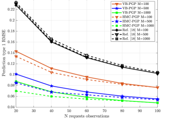
Figure 4: Prediction type 1 RMSE vs $N$ request observations

Fig. 5 shows the RMSE of the predicted popularity of unseen contents, Type 2 popularity prediction (IV-B), vs the number of observations, $N$. The features of the unseen contents are randomly generated with the same process as for the existing ones. As we see, the performance of our prediction algorithm is considerably better than the one in [18]. Again, similar to Fig. 4, the prediction accuracy improves when either $N$ or $M$ increases and also the HMC based PGP is a bit more accurate than the VB based PGP.

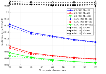
Figure 5: Prediction type 2 RMSE vs $N$ request observations

Next, we evaluate the performance of the HMC and the VB inference methods in Tables I and II. Here, we show the estimated mean values of the kernel function parameters. As we expected, it is observed that as the number of observations increases we get closer to the true values. However, from the tables, the estimation accuracy improvement of the parameters is largely affected by the number of contents. For example, for feature $x_{m}^{(2)}$, which does not affect the popularities, the estimation of its scale variation, ${\alpha_{2}}$, is better at $N=80$ for $M=500$ in comparison with $M=100$. Moreover, it can be seen that the HMC has better estimation accuracy with respect to the VB. These results confirm our previous simulations where as $M$ increases, the Gaussian process gets more accurate and consequently shows a better prediction performance.

	N=20		N=80
	HMC	VB	HMC	VB	True value
${\eta}$	0.0044	0.0232	0.0021	0.0073	0.0001
${\alpha_{0}}$	0.1299	0.0888	0.1258	0.1519	0.1
${\alpha_{1}}$	0.2179	0.1819	0.2259	0.2289	0.25
${\alpha_{2}}$	0.0199	0.0502	0.0109	0.0086	0
${\alpha_{3}}$	0.0961	766.6762	0.0642	0.0591	0.1
${\alpha_{4}}$	0.3948	0.4009	0.4375	0.4266	0.5

TABLE I: The estimates of the kernel function parameters for $M=100$

	N=20		N=80
	HMC	VB	HMC	VB	True value
${\eta}$	0.0013	0.0160	0.0002	0.0052	0.0001
${\alpha_{0}}$	0.1260	0.1295	0.1221	0.1388	0.1
${\alpha_{1}}$	0.2382	0.1568	0.2298	0.1963	0.25
${\alpha_{2}}$	0.0035	0.0041	0.0031	0.0032	0
${\alpha_{3}}$	0.0751	0.0626	0.0936	0.0799	0.1
${\alpha_{4}}$	0.4890	0.4069	0.4986	0.4274	0.5

TABLE II: The estimates of the kernel function parameters for $M=500$

V-B Caching gain Performance

In this subsection, we investigate how the prediction performance of our model affects the CHR when using the caching policy defined in (1). Throughout this subsection, we set $M=500$ and $N=40$ unless otherwise stated. In addition, the cache capacity is shown as the percentage of the total size of all contents. In the following, we respectively evaluate the CHR on synthetically generated requests and a real-world dataset.

To generate synthetic data, we use the model (10) rather than (9), since it gives more flexibility to study the influence of users’ behavior on the CHR. For simplicity, we assume that the parameters of the kernel function in (III-B) are the same for all users with ${\beta_{pu}}=1$ and also the content features are generated as previously. The $P$ user features are generated randomly as:

$${{\bf{p}}_{u}}\sim{\rm Dirichlet}\left(\omega\right),\quad\forall u=1,...,U$$ (38)

where ${\rm Dirichlet}\left(\omega\right)$ is a symmetric Dirichlet distribution with parameter $\omega$. By properly tuning $\omega$, we can control the similarity between user features. More specifically, if $\omega$ is set to be large, then the generated samples from (38) are very much alike which means that all users have more or less the same features and thus become highly correlated. On the other hand, if $\omega$ is set to be small, then the generated samples correspond to the sparse case in which each user only has a small number of features. In this case, by setting $P$ to be large, users almost have non-overlapping features which we can assume more or less they are dissimilar. In the simulations, we set $P=100$. Moreover the number of users, $U$, is $10$ and the sizes of the contents are randomly generated from the interval $\left({0,100}\right)$. In addition, we can generate popularities which mimic the Zipf distribution by tuning $\alpha_{0}$ while the other parameters are fixed. For example, Fig. 6 depicts the ranked normalized versions of the following generated popularities:

$${r_{m}}\left({{{\bf{x}}_{m}}}\right)=\sum\limits_{u=1}^{U}{{e^{{\lambda_{m}}\left({{{\bf{x}}_{m}},{{\bf{p}}_{u}}}\right)}}},\quad\forall m=1,...,M$$ (39)

with $\omega=1$ and different values of $\alpha_{0}$. The figures show that as $\alpha_{0}$ decreases the distribution of the ranked popularities converges to a Zipf distribution with small peakiness parameter.

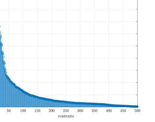
(a) $\alpha_{0}=5$

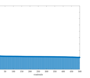
(b) $\alpha_{0}=0.001$

Figure 6: Samples from a Gaussian process to generate content popularities

In all the subsequent figures, a partially random benchmark caching strategy denoted by ”MLE-Rand” is also depicted in which we split the cache memory in two parts: $80\%$ is assigned for the seen contents with their popularities estimated by (2) and $20\%$ for randomly selecting the unseen contents. Fig. 7 shows the CHR vs the cache capacity for $\alpha_{0}=2.5$ and $\omega=1$. As we expected, CHR increases as the cache capacity increases. It can be observed that the PGP model based caching outperforms the other caching methods in this cache capacity range. For example, for cache capacity at $0.3$, the VB-PGP and HMC-PGP assisted caching improve the CHR by $8\%$ and $17\%$ with respect to [18] and MLE-Rand methods respectively. In addition, both CHR performances based on our models, HMC-PGP and VB-PGP, are very close to each other.

Fig. 8 illustrates CHR versus $\alpha_{0}$ for different values of $\omega$. The cache capacity is $0.2$ of the total size of contents. It can be seen that as $\alpha_{0}$ increases the CHR also gradually increases. This is expected since as $\alpha_{0}$ increases the distribution of content popularities becomes more like a Zipf with a large peakiness parameter (Fig. 6) meaning that only a few contents have significant contribution to the CHR gain and these can be easily distinguished since they are requested more than the other contents. On the other hand, for small $\alpha_{0}$ values the distribution of content popularities will be more like a uniform or a Zipf with a small peakiness parameter indicating that all contents have almost the same contribution to the CHR gain. Moreover, for a fixed and relatively large value of $\alpha_{0}$, the CHR decreases as $\omega$ decreases. This can be explained by noticing that when $\omega$ decreases the users will have different content preferences since they become uncorrelated. Therefore, by aggregating all the user requests, popularities are almost brought into uniformity indicating less CHR gain. In addition, we observe that the caching assisted by both of our methods is superior to the other ones for all scenarios. More specifically, the performance gap between the PGP based caching and the other ones increases as $\alpha_{0}$ increases. This is because for large $\alpha_{0}$, the CHR is very sensitive to the prediction accuracy and a small prediction mistake may cause a huge CHR reduction. This is also supported by our results in the previous subsection where we showed that our model provides higher prediction accuracy with respect to the other methods. On the other hand, for small $\alpha_{0}$ the prediction accuracy will have a small effect on the CHR.

Finally, we show the CHR performance based on our model on the real-world MovieLens 20M dataset [30]. This consists of $18$ movie genres (action, adventure, animation, children’s, comedy and so on). From the dataset, we choose ratings over 2 years, 2010 and 2011. Similar to [9], a movie’s rate is considered as one request for this movie. The length of the time slots is considered as one day. In addition, we observed that the movie popularities are almost constant during every two months of this period which indicates that our model can be applied in order to learn (almost) stationary content request distributions as underlined in the beginning of Section II. Therefore, in our simulations, the 2-year time interval is separated in $12$ bimonthly intervals where for each one the model is trained with the request observations of 30 days ($N=30$) and the CHR is evaluated during the next 30 days. Fig. 9 illustrates the CHR vs the cache capacity. Again, it can be seen that our model has a better prediction accuracy and consequently improved CHR with respect to both the MLE-Rand method and the one presented in [18]. For instance, for the cache capacity at $0.3$, our method improves CHR by $6\%$ and $11\%$ compared to the method in [18] and the MLE-Rand method respectively.

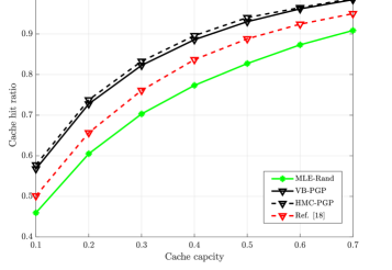
Figure 7: CHR vs cache capacity for $\alpha_{0}=2.5,\omega=1$

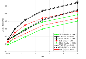
Figure 8: CHR vs $\alpha_{0}$

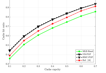
Figure 9: CHR vs cache capacity on MovieLens Dataset

VI Conclusions

In this paper, we proposed a flexible model for modeling the content requests and predicting their popularity. We proposed a multilevel probabilistic model, the Poisson regressor based on a Gaussian process, that can exploit the content features and provide accurate popularity estimation. For the seen contents, the Gaussian process acts as a regularizer which results in better estimation of their popularities. When new unseen content is introduced in the library, the proposed model can predict its popularity based on its correlation with the existing seen contents. We utilized Bayesian learning to obtain the parameters of the model because it is robust against overfitting and therefore efficient in edge-caching systems where overfitting is a big challenge due to the small number of request observations. Because the posterior distribution is not in closed form, we resort to approximation methods: the HMC sampling and the VB learning. In the simulation results, we showed that both techniques have good performance for our PGP model. Particularly, the VB is less computationally intensive than the HMC, but also a bit less accurate. Finally, we compared our method with the state-of-the-art popularity estimation scheme and showed that our method improves performance significantly.

References

- [1] C. V. N. Index, “Global mobile data traffic forecast update, 2016–2021 white paper, accessed on may 2, 2017.”
- [2] K. Shanmugam, N. Golrezaei, A. G. Dimakis, A. F. Molisch, and G. Caire, “Femtocaching: Wireless content delivery through distributed caching helpers,” IEEE Trans. Inf. Theory, vol. 59, no. 12, pp. 8402–8413, 2013.
- [3] X. Ge, H. Cheng, M. Guizani, and T. Han, “5G wireless backhaul networks: challenges and research advances,” IEEE Network, vol. 28, no. 6, pp. 6–11, 2014.
- [4] Z. Chen, J. Lee, T. Q. Quek, and M. Kountouris, “Cooperative caching and transmission design in cluster-centric small cell networks,” IEEE Trans. Wireless Commun., vol. 16, no. 5, pp. 3401–3415, 2017.
- [5] X. Peng, J. Shen, J. Zhang, and K. B. Letaief, “Joint data assignment and beamforming for backhaul limited caching networks,” in 2014 IEEE 25th Annual International Symposium on Personal, Indoor, and Mobile Radio Communication (PIMRC), Sept 2014, pp. 1370–1374.
- [6] T. X. Vu, S. Chatzinotas, and B. Ottersten, “Edge-caching wireless networks: Performance analysis and optimization,” IEEE Trans. Wireless Commun, vol. 17, no. 4, pp. 2827–2839, April 2018.
- [7] M. A. Maddah-Ali and U. Niesen, “Fundamental limits of caching,” IEEE Trans. Inf. Theory, vol. 60, no. 5, pp. 2856–2867, 2014.
- [8] W. Han, A. Liu, and V. K. Lau, “PHY-caching in 5G wireless networks: Design and analysis,” IEEE Commun. Mag., vol. 54, no. 8, pp. 30–36, 2016.
- [9] S. Müller, O. Atan, M. van der Schaar, and A. Klein, “Context-aware proactive content caching with service differentiation in wireless networks,” IEEE Trans. Wireless Commun, vol. 16, no. 2, pp. 1024–1036, 2017.
- [10] J. Song, M. Sheng, T. Q. Quek, C. Xu, and X. Wang, “Learning-based content caching and sharing for wireless networks,” IEEE Trans. Commun., vol. 65, no. 10, pp. 4309–4324, 2017.
- [11] A. Sadeghi, F. Sheikholeslami, and G. B. Giannakis, “Optimal and scalable caching for 5G using reinforcement learning of space-time popularities,” IEEE J. Sel. Topics Signal Process., vol. 12, no. 1, pp. 180–190, 2018.
- [12] S. O. Somuyiwa, A. György, and D. Gündüz, “A reinforcement-learning approach to proactive caching in wireless networks,” IEEE J. Sel. Topics Signal Process., vol. 36, no. 6, pp. 1331–1344, June 2018.
- [13] M. Garetto, E. Leonardi, and V. Martina, “A unified approach to the performance analysis of caching systems,” ACM Transactions on Modeling and Performance Evaluation of Computing Systems, vol. 1, no. 3, p. 12, 2016.
- [14] B. Bharath, K. Nagananda, and H. V. Poor, “A learning-based approach to caching in heterogenous small cell networks,” IEEE Trans. Commun., vol. 64, no. 4, pp. 1674–1686, 2016.
- [15] M. S. ElBamby, M. Bennis, W. Saad, and M. Latva-Aho, “Content-aware user clustering and caching in wireless small cell networks,” arXiv preprint arXiv:1409.3413, 2014.
- [16] G. Paschos, E. Bastug, I. Land, G. Caire, and M. Debbah, “Wireless caching: Technical misconceptions and business barriers,” IEEE Commun. Mag., vol. 54, no. 8, pp. 16–22, 2016.
- [17] E. Baştuğ, M. Bennis, and M. Debbah, “A transfer learning approach for cache-enabled wireless networks,” in Modeling and Optimization in Mobile, Ad Hoc, and Wireless Networks (WiOpt), 2015 13th International Symposium on. IEEE, 2015, pp. 161–166.
- [18] K. N. Doan, T. Van Nguyen, T. Q. Quek, and H. Shin, “Content-aware proactive caching for backhaul offloading in cellular network,” IEEE Trans. Wireless Commun., vol. 17, no. 5, pp. 3128–3140, 2018.
- [19] Y. Jiang, M. Ma, M. Bennis, F. Zheng, and X. You, “User preference learning based edge caching for Fog-RAN,” arXiv preprint arXiv:1801.06449, 2018.
- [20] L. Breslau, P. Cao, L. Fan, G. Phillips, and S. Shenker, “Web caching and zipf-like distributions: Evidence and implications,” in INFOCOM’99. Eighteenth Annual Joint Conference of the IEEE Computer and Communications Societies. Proceedings. IEEE, vol. 1. IEEE, 1999, pp. 126–134.
- [21] C. E. Rasmussen, “Gaussian processes in machine learning,” in Advanced lectures on machine learning. Springer, 2004, pp. 63–71.
- [22] R. M. Neal et al., “MCMC using hamiltonian dynamics,” Handbook of Markov Chain Monte Carlo, vol. 2, no. 11, p. 2, 2011.
- [23] K. B. Petersen, M. S. Pedersen et al., “The matrix cookbook,” Technical University of Denmark, vol. 7, no. 15, p. 510, 2008.
- [24] C. M. Bishop, Pattern recognition and machine learning, 5th Edition, ser. Information science and statistics. Springer, 2007.
- [25] D. J. MacKay, “Bayesian interpolation,” Neural computation, vol. 4, no. 3, pp. 415–447, 1992.
- [26] D. P. Bertsekas, Nonlinear programming. Athena scientific Belmont, 1999.
- [27] Y. Yang and M. Pesavento, “A unified successive pseudoconvex approximation framework,” IEEE Trans. Signal Process., vol. 65, no. 13, pp. 3313–3328.
- [28] J. Nocedal and S. J. Wright, Numerical optimization. Springer, 1999.
- [29] C. Robert, The Bayesian choice: from decision-theoretic foundations to computational implementation. Springer Science & Business Media, 2007.
- [30] F. M. Harper and J. A. Konstan, “The movielens datasets: History and context,” ACM Transactions on Interactive Intelligent Systems (TiiS), vol. 5, no. 4, p. 19, 2016.