Scheduling OLTP Transactions via Machine Learning

Abstract.

Current main memory database system architectures are still challenged by high contention workloads and this challenge will continue to grow as the number of cores in processors continues to increase (Yu:2014:SAE:2735508.2735511). These systems schedule transactions randomly across cores to maximize concurrency and to produce a uniform load across cores. Scheduling never considers potential conflicts. Performance could be improved if scheduling balanced between concurrency to maximize throughput and scheduling transactions linearly to avoid conflicts. In this paper, we present the design of several intelligent transaction scheduling algorithms that consider both potential transaction conflicts and concurrency. To incorporate reasoning about transaction conflicts, we develop a supervised machine learning model that estimates the probability of conflict. This model is incorporated into several scheduling algorithms. In addition, we integrate an unsupervised machine learning algorithm into an intelligent scheduling algorithm. We then empirically measure the performance impact of different scheduling algorithms on OLTP and social networking workloads. Our results show that, with appropriate settings, intelligent scheduling can increase throughput by 54% and reduce abort rate by 80% on a 20-core machine, relative to random scheduling. In summary, the paper provides preliminary evidence that intelligent scheduling significantly improves DBMS performance.

1. Introduction

Transaction aborts are one of the main sources of performance loss in main memory OLTP systems (Yu:2014:SAE:2735508.2735511). Current architectures for OLTP DBMS use random scheduling to assign transactions to threads. Random scheduling achieves uniform load across CPU cores and keeps all cores occupied. For workloads with a high abort rate, a large portion of work done by CPU is wasted. In contrast, the abort rate drops to zero if all transactions are scheduled sequentially into one thread. No work is wasted through aborts, but the throughput drops to the performance of a single hardware thread. Research has shown that statistical scheduling of transactions using a history can achieve low abort rate and high throughput (ZhangICDE2018) for partitionable workloads. We propose a more systematic machine learning approach to schedule transactions that achieves low abort rate and high throughput for both partitionable and non-partitionable workloads.

The fundamental intuitions of this paper are that (i) the probability that a transactions will abort will high probability can be modeled through machine learning, and (ii) given that an abort is predicted, scheduling can avoid the conflict without loss of response time or throughput. Several research works (Bailis:2014:VLDB; Stonebraker:2007:EAE:1325851.1325981; Thomson:2012:SIGMOD; prasaad-2018) perform exact analyses of aborts of transaction statements that are complex and not easily generalizable over different workloads or DBMS architectures. Our approach uses machine learning algorithms to model the probability of aborts. Our approach is to (i) build a machine learning model that helps to group transactions that are likely to abort with each other, (ii) assign each group of transactions to a first-in-first-out (FIFO) queue, and (iii) monitor concurrency across cores and adjust for imbalances. The approach requires only a thin API to the database.

2. Challenges

The first challenge is to learn a model to predict transactions aborts. This challenge involves dataset collection, feature space design and algorithm selection. The cost of learning and maintaining a model is important, but the performance of evaluation of an instance of the model, which occurs with every new transaction, is critical. Since our target is main-memory DBMS, we limit our design space to instance evaluations that are at most linear with respect to the length of a transaction statement. Since main-memory databases are fast, we have little time to make decisions because the competitor, randomize queuing of transactions, takes O(1) time.

The second challenge is to model when transaction conflict will occur. Modeling when an abort will occur is not obvious because transactions processing is complex and data dependent. Whether a transaction will abort depends on various static factors, the concurrency control protocol, the granularity of object representation (typically a tuple) and various dynamic factors, i.e. the concurrent order of execution. The feature vector of the model must capture the relevant information for a model to accurately predict aborts.

The third challenge derives from the need to cluster transactions together in a way that increases throughput by avoiding aborts. Note that aborts in main-memory databases are cheap: reducing the number of aborts provides less benefit than in a disk-based DBMS.

The fourth challenge is the cost of running schedulers and training models. Given an efficient and accurate model that predicts aborts, leveraging this information in a scheduler is not straightforward since eliminating all aborts is not necessarily the optimal policy: the scheduler must simultaneously balance (potential) aborts with a dynamically changing degree of parallelism to maximize throughput.

Finally, the approach must generalize over workloads that are not easily partitionable. We contend that, properly designed, an intelligent scheduler will reduce aborts and increase throughput relative to random scheduling.

The contributions of this paper are the following:

• We demonstrate an efficient machine learning model that predicts aborts for a pair of transactions with high accuracy.

• We present transaction scheduling methods that are largely independent of the internal logic of the DBMS and thus the methods can be easily adopted to any DBMS. The method has a low cost of engineering effort.

• We present several scheduling algorithms based on supervised and unsupervised machine learning algorithms that result in lower abort rate and higher throughput than the state of the art (random scheduling).

• We show that intelligent scheduling algorithms achieve higher throughput even when the workload is not partitionable.

• Our implementation of the best performing intelligent scheduler requires about 500 lines of additional code.

In summary, we report preliminary results on a new approach for intelligent scheduling in a DBMS. In Section 3, we explain the system architecture and environment. In Section 4 and 5, we describe how to apply both supervised and unsupervised machine learning algorithms to the transaction scheduling problem. Section 6 describes our experimental framework on main-memory databases. Section 7 describes experimental results over three workloads. Two workloads are focused on OLTP (TPC-C (TPCC), TATP (TATP)), and one workload on social networking websites (Epinions (Epinions)). The latter benchmark workload is not easily partitionable. Section 8 discusses related work and Section 9 concludes the paper.

3. System Architecture Overview

The overall environment (Figure 1) consists of three layers – the incoming stream of transaction requests, our scheduler, and a main-memory database system. The API between the system and the database is simple, consisting of three functions: (i) the ability to capture incoming transactions, (ii) the ability to queue a transaction in a specific run queue of the database, (iii) the ability to log the SQL of two events that occur during transaction processing: a transaction abort and a transaction commit, and (iv) the ability to report real-time transaction response times. This environment and API implies our approach can be “bolted on” to any DBMS with little effort. Our system does however require that for a (non user) aborted transaction, the system can identify at least one transaction that ’caused’ the abort. Typically the causing transaction holds a lock on a row or modified the row during the aborted transaction’s execution.

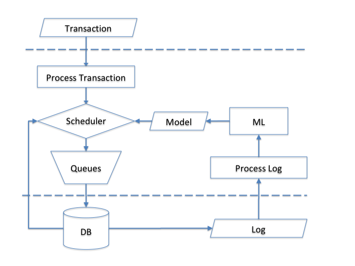
Figure 1. Functional Architecture – The Transaction component represents an incoming transaction. The Process Transaction component converts the transaction into its feature representation. The Scheduler component chooses the queue to place the incoming transaction. The Queues component represents the set of run queues. The DB component is a main-memory database system. The Log component collects transaction execution results for model training purposes. The Process Log component converts the log into its feature representation for training. The ML component trains the processed log to produce the Model. The dotted lines separate conventional components from our scheduler. The DB component also provides real-time transaction response time information to the scheduler.

4. Supervised Machine Learning

Transactions aborts are a main source of degeneration of performance in database systems. The task in this section is to design a machine learning model that detects aborts. A naive approach would be to use supervised machine learning to learn a classifier to partition transactions into two classes, Abort and Commit by simply training over log of transactions execution results. However, this approach omits the crucial fact that a transaction execution result depends on other concurrent transactions. Our approach is to learn a classifier that classifies two transactions, $T_{A}$ and $T_{B}$, into Abort if they will abort each other when run concurrently (with high probability) or Commit if they do not conflict.

4.1. Training Data

Each transaction indirectly describes information about which tuples, attributes and tables it will read and write in the database. To access this information, some works use the read/write set of a transaction, but this set of information is large and dynamically changing. Instead, the string representation of the SQL statements of a transaction are coded into a feature space. The SQL statements are a lightweight feature representation of the transaction.

4.1.1. Features

As described above, the primary goal of the model is to check if two transactions will conflict with each other. Therefore, the features should be derived from both transactions, $T_{1}$ and $T_{2}$. In particular, we want to define a function

$$trans(T_{1},T_{2})\rightarrow vector$$

to transform two transactions into a feature vector and train our model to classify this vector into Abort or Commit.

For example, in TPC-C, a transaction $T$ might want to read rows where warehouse id is equal to $10$. Then $T$ has a reference W_ID=10 and the string W_ID=10 is considered as a feature of $T$. More precisely, any instance of attribute operator value in a WHERE clause of a SELECT, DELETE or UPDATE statement is a feature. All values of an INSERT are also features. We do not distinguish between reads and writes. If $T$ both read and write rows W_ID=10, it has only one such string. The function $Features(string)\rightarrow F$ maps from a SQL string to a set of features $F$. Note that any particular transaction produces only a few features.

To produce a compact representation with a fixed size independent of the size of the transaction, we apply feature hashing, a fast and space-efficient way of converting an arbitrary number of features into indices in a fix-size vector. The function $Hash(T)$ constructs the union of the set of the features $F$ of the statements of the transaction and generates a binary vector of fixed length $k$. Given two transactions $T_{1}$ and $T_{2}$, we now have two vectors $Hash(Features(T_{1}))=V_{1}$ and $Hash(Features(T_{2}))=V_{2}$. Let $V_{3}=V_{1}\&V_{2}$ be the binary logical AND of $V_{1}$ and $V_{2}$. The final feature vector is the concatenation of these three vectors,

$$trans(T_{1},T_{2})=V_{1}|V_{2}|V_{3}$$

The vector $V_{3}$ encodes tuples, columns or tables that will potentially be touched by both transactions $T_{1}$ and $T_{2}$. In our experiments our feature vectors are 1k bits in length.

4.1.2. Canonical Features

Attribute names that appear in a schema are arbitrary, independent of the underlying domain concept. For instance, in TPC-C benchmark, the column W_ID in WAREHOUSE table and D_W_ID in DISTRICT table both represent warehouses in this database. However, their string representations in SQL are not the same (W_ID=1 and D_W_ID=1). While they express the same entity, based on the hashing function described in previous section, these two strings hash to different indices in the feature vector (baring collision). Research has shown that canonical features are more favorable than literal strings for representing transactions (ZhangICDE2018). Therefore, we adopt canonical features converting string representations of attributes to a canonical version.

Suppose a TPC-C $NewOrder$ transaction contains following SQL statements:

 SELECT W_NAME, W_STREET_1, W_STREET_2, W_CITY,
 FROM WAREHOUSE WHERE W_ID = 10
 ...
 SELECT D_NAME, D_STREET_1, D_STREET_2, D_CITY
 FROM DISTRICT WHERE D_W_ID = 10 AND D_ID = 4
 ...

Then the feature representation for these two SQL statements is:

W_ID = 10,..., W_ID = 10, D_ID = 4, ...

That is, each of these three strings is hashed and the corresponding bit is turned on in the feature vector. This representation discards most of the meaning of the SQL query and concentrates on representing only the read/write footprint of the transaction. The representation is invariant to the ordering of expressions in conjunctions and disjunctions. More complex SQL expressions, such as range expressions, are reserved for future work.

4.1.3. Training

Training data is gathered by observing the log while the system is running. Every time a transaction commits or aborts, the event is logged as one of two possible abstract triples:

• (Aborted Transaction, Conflicting Transaction, label abort)

• (Committed Transaction, Any Concurrent Transaction, label commit)

Sampling the log under random scheduling generates a distribution of transactions and abort/commit independently of our subsequent scheduling decisions. Concretely, if $T_{1}$ is aborted by $T_{2}$, then we log the pair $(trans(T_{1},T_{2}),1)$ into our log where $1$ indicates an abort. To obtain vectors in the commit set, we used the following approach: when $T_{1}$ commits, we randomly pick a transaction, $T_{2}$, that is running currently with $T_{1}$ and add $(trans(T_{1},T2),0)$ into our log. The log serves directly as the training and test set for choosing a learning algorithm.

Note that only one conflicting transaction is chosen to record in the log. However, since the choice is random, the log implicitly records a random sample of the distribution of conflicting transactions, exactly in proportion to their occurrence in the workload.

Moreover this feature encoding intentionally ignores many details of the transaction process system: the type of concurrency control regime, the level of conflict detection (partition, tuple, field, object, page), etc. All these issues are treated as a “black box” by the machine learning model. The model learns which features are relevant to modeling abort probabilities as given by the log. Thus, our approach is applicable to a wide range of systems.

4.1.4. Model Evaluation

We will assume that the hypothesis space is linear and defer non-linear models for future work. Our learning algorithm needs to be cheap to train and very fast to evaluate on a pair of transactions. Logistic regression is both cheap to train and can evaluate an example in $O(n)$ time where $n$ is the number of 1 bits in the feature vector, using a sparse representation. Example evaluation time is proportional to the sum of the string lengths of the two transactions. In practice $n$ is small (less than 20) and the evaluation consists of multiplication of each 1 feature vector bit by a scalar and summing to produce a final score. Another advantage is that the score for logistic regression can be interpreted as the probability that the transaction pair will produce an abort. The trained model generates parameters for a function

$$M(T_{1},T_{2})\rightarrow P(commit/abort)$$

that predicts abort probabilities for any transaction pair $(T_{1},T_{2})$.

4.1.5. Model Accuracy

With a large set of transaction abort instances, we use 4-fold cross-validation to learn and evaluate the accuracy of the models. We set the training size to include 10,000 training data points for each benchmark. Logistic regression (Table 4.1.5) performs well for all three benchmarks.

Model Accuracy
Benchmark	Training Size	Accuracy	Majority
AP	10,000	0.966	0.500
PC-C & 10,000 & 0.985 & 0.500\\ \verb Epinions & 10,000 & 0.951 & 0.500\\ \multicolumn{3}{c}{ } \\ % make some space between tables \end{tabular} \caption{Logistic Regression Accuracy. he Accuracy column reports the accuracy of the logistic regression classifier. For comparison, the Majority column reports the accuracy of a classify that chooses the majority class of the training data. 4.2. Scheduling Algorithms Our task in this section is to design an algorithm using $M$ that assigns a transaction, $T_{new}$, into a queue in a way that avoids aborts and increases throughput compared to random scheduling. Consider a transaction $T_{k}$ already queued and waiting to execute. Suppose $M(T_{new},T_{k})$ has low abort probability. A low abort probabilities does not make it clear which queue to assign $T_{new}$ since some other concurrent transaction may have a high abort probability. Suppose $M(T_{new},T_{k})$ predicts a high abort probability. Then if these two transactions run concurrently, with high probability at least one abort will occur, perhaps two (depending on the details of the concurrency control system). Assigning transaction $T_{new}$ into a different queue than $T_{k}$ may succeed as long as the database does not try to execute them at the same time. Concurrent execution depends in this case on there being the same amount of work in front of each queued transaction, so that they both arrive to the front of the queue at the same time, and are processed concurrently. However, predicting the total work in a queue is difficult. The simplest heuristic places $T_{new}$ into the same FIFO queue after $T_{k}$ so they never execute concurrently. With this heuristic in mind, the algorithm computes $$Enqueue(T_{new},queue(\operatorname*{argmax}_{T_{i}}M(T_{new},T_{i}))$$ where $queue(T)$ is a function that returns the queue of transaction $T$. That is, for a new transaction $T_{new}$, search for $T_{high}$ in some queue with the highest abort probability $M(T_{new},T_{high})$, then assign $T_{new}$ to the same queue as $T_{high}$ (algorithm 1). Algorithm 1 Assign($T_{new}$) $p=-1$ $q=-1$ for $T\in\mathbb{T}$ do      if $M(T_{new},T)>p$ then          $p=M(T_{new},T)$          $q=queue(T)$      end if end for if $p>-1$ then      Assign $T_{new}$ to FIFO $q$ else      Assign $T_{new}$ randomly end if 4.2.1. Search Scheduling Algorithm Usually, more than one scheduler assigns transactions concurrently. In this case, two schedulers respective inflight transactions might conflict. Dealing with this case would require the schedulers to check if their transactions conflict, requiring a costly coordination between schedulers. Finally, for efficiency purposes, if a high probability abort is discovered (above $\theta=0.5$), the search is stopped early and the current $T$ is treated as $T_{high}$. The new transaction is added to the end of $T$’s queue. To prevent bias towards one queue or another, we randomize the starting queue for the search. We can search queues in two different ways: Breadth First Search (BFS) and Depth First Search (DFS). Extensive analysis and experimentation have shown that DFS performs poorly compared to BFS. DFS spends much more time searching for high probability transactions. Suppose we have $n$ queues, $q_{0},q_{2},...q_{n-1}$. The pseudo code for assigning $T_{new}$ using BFS scheduling (algorithm 2) is below. The code assumes that $ID(T)$ returns the identifier of $T$ which is also a timestamp of the starting time of the transaction. Algorithm 2 BFSAssign($T_{new}$) ${id\_set}=\{\}$ ${q\_set}=\{\}$ $\alpha\leftarrow Random(0,n-1)$ while $Size({q\_set})<n$ do      for $i:=0$ to $n-1$ do          $j\leftarrow\alpha+i\;\;{mod}\;\;\;n$          if $j\in{q\_set}$ then               continue          end if          $T_{head}\leftarrow Dequeue(q_{j})$          if $T_{head}=={NULL}$ then               ${q\_set}\leftarrow{q\_set}\cup\{j\}$               continue          end if          if $ID(T_{head})>ID(T_{new})\;\;||\;\;ID(T_{head})\in{id\_set}$ then               $Enqueue(q_{j},T_{head})$               ${q\_set}\leftarrow{q\_set}\cup\{j\}$               continue          end if          ${id\_set}\leftarrow{id\_set}\cup\{ID(T_{head})\}$          $p\leftarrow M(T_{new},T_{head})$          $Enqueue(q_{j},T_{head})$          if $p>\theta$ then               $Enqueue(q_{j},T_{new})$               return          end if      end for end while $Enqueue(q_{\alpha},T_{new})$ The worst case computation cost, in terms of model evaluations, for both algorithms is $O(n)$ where $n$ is the number of waiting transactions. This cost is paid by every queued transaction. The combination of the model evaluation and the heuristic of scheduling aborts into the same queue will tend to group high probability conflicting transactions into the same queue. We can exploit this behavior to reduce the computation cost of finding the best queue to schedule a transaction collapsing the feature vectors of the transactions in the queue to a centroid that represents the “average” transaction. 4.2.2. Balanced Vector Scheduling Algorithm The Vector scheduler creates a representative transaction $R_{i}$ for the history of transactions in each queue $q_{i}$. $R_{i}$ represents transactions in $q_{i}$ by averaging the feature vectors of the transactions enqueued into $q_{i}$. That is, the features of transaction are bit vectors but the centroid representing each queue is a vector of floats. The model $M$ remains unchanged for training purposes. The difference is in instance evaluation. To determine the best queue for a new transaction $T_{new}$ the algorithm computes $$Enqueue(T_{new},\operatorname*{argmax}_{i}=M(T_{new},R_{i}))$$ The computational cost in terms of model evaluations is $O(n)$ where $n$ is the number of queues in the system. When we assign $T_{new}$ to $q_{i}$, we need to update $R_{i}$. This update requires latches to insure consistency of the update in the case of multiple schedulers. The results section describes the empirical cost of this contention. The random schedule insures a balanced workload across the system. The $BFS$ scheduler somewhat balances workload due to scheduling into empty queues. The $Vector$ scheduler described above does not possess this property. To balance the workload, we additionally track the average response time for transactions coming from each queue, as well as the standard deviation. If a queue has too many transactions, the average transaction response time will increase drastically and exceed a reasonable response time limitation, which we define to be one standard deviation higher than the average response time. If the response time of queue with the highest abort probability is above this limit, the queue is blocked from receiving new transactions. The queue is unblocked when it is empty. The new transaction is assigned to the unblocked queue with lowest response time. Noe that the $R$ vector is updated during an enqueue but not a dequeue. So $R$ represents a history of transactions scheduled into the queue and thus represents a centroid of the feature vectors of the history. The $Balanced$ $Vector$ $Assign$ scheduler (algorithm 3) attempts to trade off high abort probability with a balanced workload. In the algorithm, $R[i]$ is the sum of all the vectors that have been enqueued in $q_{i}$ and $R_{avg}[i]$ is the average of all the vectors that have been enqueued in $q_{i}$. Both $R[i]$ and $R_{avg}[i]$ are zero vectors when the system initially starts. Algorithm 3 BalancedVectorAssign($T_{new}$) ${max\_prob}\leftarrow 0$ ${idx}\leftarrow-1$ $V_{new}\leftarrow Hash(T_{new})$ for $i:=0$ to $n-1$ do      $P\leftarrow M^{\prime}(V_{new},R_{avg}[i])$      if $P\geq{max\_prob}$ then          ${max\_prob}\leftarrow P$          ${idx}\leftarrow i$      end if end for ${rt}\leftarrow GetResTimeHistory(q_{{idx}})$ ${rt\_avg}\leftarrow GetResTimeAvg(rt)$ ${rt\_std}\leftarrow GetResTimeStd(rt)$ if ${rt-rt\_avg}>{rt\_std}$ then      ${min\_rt}\leftarrow\infty$      for $i:=0$ to $n-1$ do          ${rt\_i}\leftarrow GetResTimeHistory(q_{i})$          if ${rt\_i}<{min\_rt}$ then               ${min\_rt}\leftarrow{rt\_i}$               ${idx}\leftarrow i$          end if      end for end if $Count[{idx}]\leftarrow Count[{idx}]+1$ $R[{idx}]\leftarrow R[{idx}]+V_{new}$ $R_{avg}[idx]\leftarrow R[{idx}]/Count[{idx}]$ $Enqueue(q_{{idx}},T_{new})$ 4.3. Supervised Scheduler Summary In summary, the transactions assignment execution time of BFS is $O(n)$ where $n$ is the number of queued transactions, less the early stop criterion of finding a younger transaction or finding a high abort probability transaction. The transaction execution time of Balanced Vector Assign is $O(kd)$ where $k$ is the number of queues, $d$ is the length of the feature vector (in a dense representation of floats), plus some additional cost for detecting imbalances in response times. The vector centroids are updated with each newly queued transaction (but not on transaction commit) and thus represent a history of transactions.