The Variational Predictive Natural Gradient

Abstract

Variational inference transforms posterior inference into parametric optimization thereby enabling the use of latent variable models where otherwise impractical. However, variational inference can be finicky when different variational parameters control variables that are strongly correlated under the model. Traditional natural gradients based on the variational approximation fail to correct for correlations when the approximation is not the true posterior. To address this, we construct a new natural gradient called the Variational Predictive Natural Gradient (VPNG). Unlike traditional natural gradients for variational inference, this natural gradient accounts for the relationship between model parameters and variational parameters. We demonstrate the insight with a simple example as well as the empirical value on a classification task, a deep generative model of images, and probabilistic matrix factorization for recommendation.

1 Introduction

Variational inference (Jordan et al., 1999) transforms posterior inference in latent variable models into optimization. It posits a parametric approximating family and tries to find the distribution in this family that minimizes the Kullback-Leibler (kl) divergence to the posterior. Variational inference makes posterior computation practical where it would not be otherwise. It has powered many applications, including computational biology (Carbonetto et al., 2012; Stegle et al., 2010), language (Miao et al., 2016), compressive sensing (Shi et al., 2014), neuroscience (Manning et al., 2014; Harrison & Green, 2010), and medicine (Ranganath et al., 2016).

Variational inference requires choosing an approximating family. The variational family plus the model together define the variational objective. The variational objective can be optimized with stochastic gradients for a broad range of models (Kingma & Welling, 2014; Ranganath et al., 2014; Rezende et al., 2014). When the posterior has correlations, dimensions of the optimization problem become tied, i.e., there is curvature. One way to correct for curvature in optimization is to use natural gradients (Amari, 1998; Ollivier et al., 2011; Thomas et al., 2016) . Natural gradients for variational inference (Hoffman et al., 2013) adjust for the non-Euclidean nature of probability distributions. But they may not change the gradient direction when the variational approximation is far from the posterior.

To deal with curvature induced by dependent observation dimensions in the variational objective, we define a new type of natural gradient: the variational predictive natural gradient (vpng). The vpng rescales the gradient with the inverse of the expected Fisher information matrix of the reparameterized model likelihood. We relate this matrix to the negative Hessian of the expected log-likelihood part of the evidence lower bound (elbo), thereby showing it captures the curvature of variational inference.

Our new natural gradient captures potential pathological curvature introduced by the log-likelihood traditional natural gradient cannot capture. Further, unlike traditional natural gradients for variational inference, the vpng corrects for curvature in the objective between model parameters and variational parameters. In Section 3, we will design an illustrate example where the vpng points almost directly to the optimum, while both the vanilla gradient and the natural gradient point in almost an orthogonal direction.

We show our approach outperforms vanilla gradient optimization and the traditional natural gradient optimization on several latent variable models, including Bayesian logistic regression on synthetic data, variational autoencoders (Kingma & Welling, 2014; Rezende et al., 2014) on images, and variational probabilistic matrix factorization (Mnih & Salakhutdinov, 2008; Gopalan et al., 2015; Liang et al., 2016) on movie recommendation data.

Related work.

Variational inference has been transformed by the use of Monte Carlo gradient estimators  (Kingma & Ba, 2014; Rezende et al., 2014; Mnih & Gregor, 2014; Ranganath et al., 2014; Titsias & Lázaro-Gredilla, 2014). Though these approaches expand the applicability of variational inference, the underlying optimization problem can still be hard. Some recent work applied second-order optimization to solve this problem. For example, Fan et al. (2015) derived Hessian-free style optimization for variational inference. Another line of related work is on efficiently computing Fisher information and natural gradients for complex model likelihood such as the K-FAC approximation  (Martens & Grosse, 2015; Grosse & Martens, 2016; Ba et al., 2016). Finally, the vpng can be combined with methods for robustly setting step sizes, like using the vpng curvature matrix to build the quadratic approximation in TrustVI (Regier et al., 2017).

2 Background

Latent variable models

Latent variable models posit latent structure ${\boldsymbol{\mathbf{z}}}$ to describe data ${\boldsymbol{\mathbf{x}}}$ with parameters ${\boldsymbol{\mathbf{\theta}}}$. The model is

$$p({\boldsymbol{\mathbf{x}}},{\boldsymbol{\mathbf{z}}})=p({\boldsymbol{\mathbf{z}}})p({\boldsymbol{\mathbf{x}}}\,|\,{\boldsymbol{\mathbf{z}}};{\boldsymbol{\mathbf{\theta}}}).$$

The model is split into a prior over the hidden structure $p({\boldsymbol{\mathbf{z}}})$ and likelihood that describes the probability of data.

Variational inference

Variational inference (Jordan et al., 1999) approximates the posterior distribution $p({\boldsymbol{\mathbf{z}}}\,|\,{\boldsymbol{\mathbf{x}}};{\boldsymbol{\mathbf{\theta}}})$ with a distribution $q({\boldsymbol{\mathbf{z}}}\,|\,{\boldsymbol{\mathbf{x}}};{\boldsymbol{\mathbf{\lambda}}})$ over the latent variables indexed by parameter ${\boldsymbol{\mathbf{\lambda}}}$. It works by maximizing the elbo:

$$\mathcal{L}({\boldsymbol{\mathbf{\lambda}}},{\boldsymbol{\mathbf{\theta}}})=\mathbb{E}_{q}\left[\log p({\boldsymbol{\mathbf{x}}}\,|\,{\boldsymbol{\mathbf{z}}};{\boldsymbol{\mathbf{\theta}}})\right]-\textrm{KL}(q({\boldsymbol{\mathbf{z}}}\,|\,{\boldsymbol{\mathbf{x}}};{\boldsymbol{\mathbf{\lambda}}})||p({\boldsymbol{\mathbf{z}}}))$$ (1)

Maximizing the elbo minimizes the kl divergence to the posterior. The model parameters ${\boldsymbol{\mathbf{\theta}}}$ and variational parameters ${\boldsymbol{\mathbf{\lambda}}}$ can be optimized together. The family $q$ is chosen to be amenable to stochastic optimization. One example is the mean-field family, where $q({\boldsymbol{\mathbf{z}}}\,|\,{\boldsymbol{\mathbf{x}}})$ is factorized over all coordinates of ${\boldsymbol{\mathbf{z}}}$ like in the variational autoencoder.

$q$-Fisher information

The elbo can be optimized with gradients. The effectiveness of gradient ascent methods relates to the geometry of the problem. When the loss landscape contains variables that control the objective in a coupled manner, like the means of two correlated latent variables, gradient ascent methods can be slow.

One way to adjust for this coupling or curvature is to use natural gradients (Amari, 1998). Natural gradients account for the non-Euclidean geometry of parameters of probability distributions by looking for optimal ascent directions in symmetric KL-divergence balls. The natural gradient relies on the Fisher information of $q$,

$$F_{q}=\mathbb{E}_{q}\left[\nabla_{\boldsymbol{\mathbf{\lambda}}}\log q({\boldsymbol{\mathbf{z}}}|{\boldsymbol{\mathbf{x}}};{\boldsymbol{\mathbf{\lambda}}})\cdot\nabla_{\boldsymbol{\mathbf{\lambda}}}\log q({\boldsymbol{\mathbf{z}}}|{\boldsymbol{\mathbf{x}}};{\boldsymbol{\mathbf{\lambda}}})^{\top}\right].$$ (2)

We call this matrix the $q$-Fisher information matrix. With this Fisher information matrix, the natural gradient is $\nabla_{\boldsymbol{\mathbf{\lambda}}}^{\lx@glossaries@gls@link{acronym}{NG}{\leavevmode\textsc{ng}}}\mathcal{L}({\boldsymbol{\mathbf{\lambda}}})~{}=~{}F_{q}^{-1}\cdot\nabla_{\boldsymbol{\mathbf{\lambda}}}\mathcal{L}({\boldsymbol{\mathbf{\lambda}}})$.

Natural gradients have been used to optimize the the elbo (Hoffman et al., 2013). The natural gradient works because it approximates the Hessian of the elbo at the optimum. The negative Hessian matrix of the elbo is:

$$-\frac{\partial^{2}}{\partial{\boldsymbol{\mathbf{\lambda}}}^{2}}\mathcal{L}=F_{q}+ \int\frac{\partial^{2}}{\partial{\boldsymbol{\mathbf{\lambda}}}^{2}}q\cdot(\log q({\boldsymbol{\mathbf{z}}}\,|\,{\boldsymbol{\mathbf{x}}};{\boldsymbol{\mathbf{\lambda}}})-\log p({\boldsymbol{\mathbf{z}}}\,|\,{\boldsymbol{\mathbf{x}}}))d{\boldsymbol{\mathbf{z}}}.$$ (3)

The last integral in the above equation is small when the variational distribution $q({\boldsymbol{\mathbf{z}}}\,|\,{\boldsymbol{\mathbf{x}}};{\boldsymbol{\mathbf{\lambda}}})$ is close to the posterior distribution $p({\boldsymbol{\mathbf{z}}}\,|\,{\boldsymbol{\mathbf{x}}})$. Hence, the $q$-Fisher information matrix can be viewed as a positive semi-definite version of the negative Hessian matrix of the elbo. Thus natural gradients improve optimization efficiency, when the variational approximation is close to the posterior.

3 The Variational Predictive Natural Gradient

The $q$-Fisher information is insufficient.

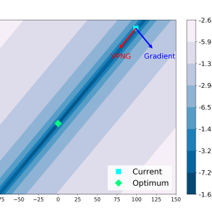
Figure 1: The vpngs are more effective than vanilla gradients and traditional natural gradients (pointing into the same direction with the vanilla gradients for this example).

Consider the following example with bivariate Gaussian likelihood that has an unknown mean ${\boldsymbol{\mathbf{\mu}}}=\begin{pmatrix}\mu_{1}\\ \mu_{2}\end{pmatrix}$, a pathological known covariance $\Sigma=\begin{pmatrix}1&1-\varepsilon\\ 1-\varepsilon&1\end{pmatrix}$ for some constant $0\leq\varepsilon\ll 1$, and an isotropic Gaussian prior:

$$p({\boldsymbol{\mathbf{x}}}_{1:n},{\boldsymbol{\mathbf{\mu}}}) =\ p({\boldsymbol{\mathbf{\mu}}}\,|\,{\boldsymbol{\mathbf{0}}},I_{2})\prod_{i=1}^{n}\mathcal{N}\left({\boldsymbol{\mathbf{x}}}_{i}\,|\,{\boldsymbol{\mathbf{\mu}}},\Sigma\right).$$ (4)

To do variational inference, we choose a mean-field approximation $q({\boldsymbol{\mathbf{\mu}}};{\boldsymbol{\mathbf{\lambda}}})=\mathcal{N}(\mu_{1}\,|\,\lambda_{1},\sigma^{2})\mathcal{N}(\mu_{2}\,|\,\lambda_{2},\sigma^{2})$ with $\sigma$ to be fixed. The posterior distribution for this problem is analytic: $p({\boldsymbol{\mathbf{\mu}}}|{\boldsymbol{\mathbf{x}}})=\mathcal{N}({\boldsymbol{\mathbf{\mu}}}^{\prime},\Sigma^{\prime})$ where $\Sigma^{\prime}=(n\Sigma^{-1}+I_{2})^{-1}$ and ${\boldsymbol{\mathbf{\mu}}}^{\prime}=(n\cdot I_{2}+\Sigma)^{-1}\cdot\sum_{i=1}^{n}{\boldsymbol{\mathbf{x}}}_{i}$. The optimal solution for the variational parameter ${\boldsymbol{\mathbf{\lambda}}}$ should be ${\boldsymbol{\mathbf{\mu}}}^{\prime}$. The gradient of the objective function $\mathcal{L}({\boldsymbol{\mathbf{\lambda}}})$ is

$$\nabla_{\boldsymbol{\mathbf{\lambda}}}\mathcal{L}({\boldsymbol{\mathbf{\lambda}}})=-{\boldsymbol{\mathbf{\lambda}}}+\Sigma^{-1}\cdot\left(-n{\boldsymbol{\mathbf{\lambda}}}+\sum_{i=1}^{n}{\boldsymbol{\mathbf{x}}}_{i}\right).$$ (5)

The precision matrix $\Sigma^{-1}$ is pathological. It has an eigenvector ${\boldsymbol{\mathbf{v}}}_{1}=\frac{1}{\sqrt{2}}(1,1)^{\top}$ with eigenvalue $\frac{1}{2-\varepsilon}$, and an eigenvector ${\boldsymbol{\mathbf{v}}}_{2}=\frac{1}{\sqrt{2}}(1,-1)^{\top}$ with eigenvalue $\frac{1}{\varepsilon}$. As a result, vanilla gradients will almost always go along the direction of the eigenvector ${\boldsymbol{\mathbf{v}}}_{2}$, as shown in Figure 1. Further, natural gradients fail to resolve this. The $q$-Fisher information matrix of this problem is diagonal, so it cannot help resolve the extreme curvature between the parameters $\lambda_{1}$ and $\lambda_{2}$.

Notice that this pathological curvature is not due to that mean-field approximation family on $q({\boldsymbol{\mathbf{\mu}}};{\boldsymbol{\mathbf{\lambda}}})$ does not contain the true posterior $p({\boldsymbol{\mathbf{\mu}}}\,|\,{\boldsymbol{\mathbf{x}}})$. In fact, even if we optimize $q({\boldsymbol{\mathbf{\mu}}};{\boldsymbol{\mathbf{\lambda}}})$ over the family of all bivariate Gaussian distributions $\mathcal{N}({\boldsymbol{\mathbf{\mu}}}\,|\,{\boldsymbol{\mathbf{\lambda}}}_{\boldsymbol{\mathbf{\mu}}},{\boldsymbol{\mathbf{\lambda}}}_{\Sigma})$, the partial gradient $\nabla_{{\boldsymbol{\mathbf{\lambda}}}_{\boldsymbol{\mathbf{\mu}}}}\mathcal{L}$ over the mean parameter vector ${\boldsymbol{\mathbf{\lambda}}}_{\boldsymbol{\mathbf{\mu}}}$ will still have the same curvature issue. The issue arises since the variational approximation does not approximate the posterior well at initialization . In general, if at some point the current $q$ iterate cannot approximate the posterior well, then the corresponding $q$-Fisher information matrix may not be able to correct the curvature in the parameters.

3.1 Negative Hessian of the expected log-likelihood

The pathology of the elbo for the model in Equation 4 comes from the ill-conditioned covariance matrix $\Sigma$. The covariance matrix of the posterior can correct for this pathology since its covariance matrix is $\Sigma^{\prime}\approx\frac{1}{n}\Sigma$. The disconnect lies in that variational inference is only close to the posterior at its optimum, which implies that q-natural gradients only correct for the curvature well once the variational approximation is close to the posterior, i.e., the inference problem is almost solved.

The problem is that the $q$-Fisher information matrix measures how parameter perturbations alter the variational approximation, regardless of the current model parameters and the quality of the current variational approximation. We bring the model back into the picture by considering positive definite matrices that resemble the negative Hessian matrix of the expected log-likelihood part $\mathcal{L}^{\textrm{ll}}=\mathbb{E}_{q}\left[\log p({\boldsymbol{\mathbf{x}}}\,|\,{\boldsymbol{\mathbf{z}}};{\boldsymbol{\mathbf{\theta}}})\right]$ of the elbo, over both the variational parameter ${\boldsymbol{\mathbf{\lambda}}}$ and the model parameter ${\boldsymbol{\mathbf{\theta}}}$.

The expected log-likelihood contains where the model and variational approximation interact, so its Hessian contains the relevant curvature for optimize the elbo. However, since we are maximizing the elbo, the matrices need to not only resemble the negative Hessian, but should also be positive semidefinite. The negative Hessian of the expected log-likelihood is not guaranteed to be positive semi-definite. Our goal is to construct a positive semidefinite matrix related to the negative Hessian that accelerate inference by considering the curvature both the variational parameter and the model parameter. In the sequel, we will show this new matrix is a type of Fisher information.

To compute gradients and Hessians, we need to compute derivatives over expectations controlled by the variational parameter ${\boldsymbol{\mathbf{\lambda}}}$. In general, we can differentiate and use score function-style estimators from black box variational inference (Ranganath et al., 2014). For simplicity, consider the case where $q$ is reparameterizable (Kingma & Welling, 2014; Rezende et al., 2014). Then draws for ${\boldsymbol{\mathbf{z}}}$ from $q$ can be written as deterministic transformations $g$ of noise terms ${\boldsymbol{\mathbf{\varepsilon}}}$ with parameter-free distributions $s$. This simplifies the computations:

$${\boldsymbol{\mathbf{z}}}=g({\boldsymbol{\mathbf{x}}},{\boldsymbol{\mathbf{\varepsilon}}};{\boldsymbol{\mathbf{\lambda}}})\sim q({\boldsymbol{\mathbf{z}}}\,|\,{\boldsymbol{\mathbf{x}}};{\boldsymbol{\mathbf{\lambda}}})\iff{\boldsymbol{\mathbf{\varepsilon}}}\sim s({\boldsymbol{\mathbf{\varepsilon}}}).$$ (6)

The reparameterization trick can be applied to many common distributions (i.e. reparameterize a Gaussian draw $\nu~{}\sim~{}\mathcal{N}(\mu,\sigma^{2})$ as $\nu=\mu+\sigma\varepsilon$ where $\varepsilon\sim\mathcal{N}(0,1)$).

With this trick, denote ${\boldsymbol{\mathbf{\eta}}}=({\boldsymbol{\mathbf{\lambda}}}^{\top},{\boldsymbol{\mathbf{\theta}}}^{\top})^{\top}$, the negative Hessian matrix of $\mathcal{L}^{\textrm{ll}}$ becomes:

$$-\frac{\partial^{2}\mathcal{L}^{\textrm{ll}}}{\partial{\boldsymbol{\mathbf{\eta}}}^{2}}=-\mathbb{E}_{\boldsymbol{\mathbf{\varepsilon}}}\left[\frac{\partial^{2}}{\partial{\boldsymbol{\mathbf{\eta}}}^{2}}\log p({\boldsymbol{\mathbf{x}}}\,|\,{\boldsymbol{\mathbf{z}}}=g({\boldsymbol{\mathbf{x}}},{\boldsymbol{\mathbf{\varepsilon}}};{\boldsymbol{\mathbf{\lambda}}});{\boldsymbol{\mathbf{\theta}}})\right].$$

Let us first consider the case where the variational distribution $q$ factorizes over data points: $q({\boldsymbol{\mathbf{z}}}\,|\,{\boldsymbol{\mathbf{x}}};{\boldsymbol{\mathbf{\lambda}}})=\prod_{i=1}^{n}q({\boldsymbol{\mathbf{z}}}_{i}\,|\,{\boldsymbol{\mathbf{x}}}_{i};{\boldsymbol{\mathbf{\lambda}}})$. This factorization occurs in many popular models, such as in variational autoencoders (vaes) (Kingma & Welling, 2014; Rezende et al., 2014). Denote $Q$ as the empirical distribution of the observed data ${\boldsymbol{\mathbf{x}}}_{1:n}$. Also denote $p({\boldsymbol{\mathbf{z}}}_{i})$ and $p({\boldsymbol{\mathbf{x}}}_{i}\,|\,{\boldsymbol{\mathbf{z}}}_{i})$ as the prior and likelihood function for any single data point ${\boldsymbol{\mathbf{x}}}_{i}$. Moreover, for any data point ${\boldsymbol{\mathbf{x}}}_{i}$ and ${\boldsymbol{\mathbf{x}}}^{\prime}_{i}$, we define the function

$$u({\boldsymbol{\mathbf{x}}}_{i},{\boldsymbol{\mathbf{x}}}^{\prime}_{i},{\boldsymbol{\mathbf{\varepsilon}}}_{i},{\boldsymbol{\mathbf{\eta}}})=\frac{\partial^{2}}{\partial{\boldsymbol{\mathbf{\eta}}}^{2}}\log p({\boldsymbol{\mathbf{x}}}^{\prime}_{i}\,|\,{\boldsymbol{\mathbf{z}}}_{i}=g({\boldsymbol{\mathbf{x}}}_{i},{\boldsymbol{\mathbf{\varepsilon}}}_{i};{\boldsymbol{\mathbf{\lambda}}});{\boldsymbol{\mathbf{\theta}}}).$$

Since we can use ${\boldsymbol{\mathbf{z}}}_{i}=g({\boldsymbol{\mathbf{x}}}_{i},{\boldsymbol{\mathbf{\varepsilon}}}_{i};{\boldsymbol{\mathbf{\lambda}}})$ to reparameterize ${\boldsymbol{\mathbf{z}}}_{i}$, we can assume that the Jacobian matrix $\frac{\partial{\boldsymbol{\mathbf{z}}}_{i}}{\partial{\boldsymbol{\mathbf{\varepsilon}}}_{i}}$ is always invertible and hence by the inverse function theorem we can also write ${\boldsymbol{\mathbf{\varepsilon}}}_{i}$ as a function of ${\boldsymbol{\mathbf{z}}}_{i}$, ${\boldsymbol{\mathbf{x}}}_{i}$ and ${\boldsymbol{\mathbf{\lambda}}}$. Hence, we can also express the above equation as

$$\frac{\partial^{2}}{\partial{\boldsymbol{\mathbf{\eta}}}^{2}}\log p({\boldsymbol{\mathbf{x}}}^{\prime}_{i}\,|\,{\boldsymbol{\mathbf{z}}}_{i}=g({\boldsymbol{\mathbf{x}}}_{i},{\boldsymbol{\mathbf{\varepsilon}}}_{i};{\boldsymbol{\mathbf{\lambda}}});{\boldsymbol{\mathbf{\theta}}})=v({\boldsymbol{\mathbf{x}}}_{i},{\boldsymbol{\mathbf{x}}}^{\prime}_{i},{\boldsymbol{\mathbf{z}}}_{i},{\boldsymbol{\mathbf{\eta}}}).$$

With this notation, we can rewrite the above negative Hessian matrix for $\mathcal{L}^{\textrm{ll}}$ as

$$- \frac{\partial^{2}\mathcal{L}^{\textrm{ll}}}{\partial{\boldsymbol{\mathbf{\eta}}}^{2}}=-\sum\limits_{i=1}^{n}\mathbb{\mathbb{missing}}\mathbb{E}_{{\boldsymbol{\mathbf{\varepsilon}}}_{i}}\left[\frac{\partial^{2}}{\partial{\boldsymbol{\mathbf{\eta}}}^{2}}\log p({\boldsymbol{\mathbf{x}}}_{i}\,|\,{\boldsymbol{\mathbf{z}}}_{i}=g({\boldsymbol{\mathbf{x}}}_{i},{\boldsymbol{\mathbf{\varepsilon}}}_{i};{\boldsymbol{\mathbf{\lambda}}});{\boldsymbol{\mathbf{\theta}}})\right]$$ (7)

$$=-n\mathbb{E}_{Q({\boldsymbol{\mathbf{x}}}_{i})}\left[\mathbb{E}_{{\boldsymbol{\mathbf{\varepsilon}}}_{i}}\left[\frac{\partial^{2}}{\partial{\boldsymbol{\mathbf{\eta}}}^{2}}\log p({\boldsymbol{\mathbf{x}}}_{i}\,|\,{\boldsymbol{\mathbf{z}}}_{i}=g({\boldsymbol{\mathbf{x}}}_{i},{\boldsymbol{\mathbf{\varepsilon}}}_{i};{\boldsymbol{\mathbf{\lambda}}});{\boldsymbol{\mathbf{\theta}}})\right]\right]$$

$$=-n\mathbb{E}_{Q({\boldsymbol{\mathbf{x}}}_{i})}\left[\mathbb{E}_{{\boldsymbol{\mathbf{\varepsilon}}}_{i}}\left[u({\boldsymbol{\mathbf{x}}}_{i},{\boldsymbol{\mathbf{x}}}_{i},{\boldsymbol{\mathbf{\varepsilon}}}_{i},{\boldsymbol{\mathbf{\eta}}})\right]\right]$$

$$=-n\mathbb{E}_{Q({\boldsymbol{\mathbf{x}}}_{i})}\left[\mathbb{E}_{q({\boldsymbol{\mathbf{z}}}_{i}\,|\,{\boldsymbol{\mathbf{x}}}_{i};{\boldsymbol{\mathbf{\lambda}}})}\left[v({\boldsymbol{\mathbf{x}}}_{i},{\boldsymbol{\mathbf{x}}}_{i},{\boldsymbol{\mathbf{z}}}_{i},{\boldsymbol{\mathbf{\eta}}})\right]\right]$$

Assessing the positive definiteness of Equation 7 is a challenge because of the expectation with respect to the variational approximation. To make the positive definiteness easier to wrangle, we make the assumption that

$$p({\boldsymbol{\mathbf{z}}}_{i})p({\boldsymbol{\mathbf{x}}}_{i}\,|\,{\boldsymbol{\mathbf{z}}}_{i})\approx Q({\boldsymbol{\mathbf{x}}}_{i})q({\boldsymbol{\mathbf{z}}}_{i}\,|\,{\boldsymbol{\mathbf{x}}}_{i}).$$ (8)

When our model is learning a successful parameter vector ${\boldsymbol{\mathbf{\eta}}}$, the distribution $p({\boldsymbol{\mathbf{z}}}_{i},{\boldsymbol{\mathbf{x}}}_{i})~{}=~{}p({\boldsymbol{\mathbf{z}}}_{i})p({\boldsymbol{\mathbf{x}}}_{i}\,|\,{\boldsymbol{\mathbf{z}}}_{i})$ should be close to the distribution $Q({\boldsymbol{\mathbf{z}}}_{i},{\boldsymbol{\mathbf{x}}}_{i})~{}=~{}Q({\boldsymbol{\mathbf{x}}}_{i})q({\boldsymbol{\mathbf{z}}}_{i}\,|\,{\boldsymbol{\mathbf{x}}}_{i})$ since the variational distribution $q$ is trying to learn the posterior distribution $p({\boldsymbol{\mathbf{z}}}_{i}\,|\,{\boldsymbol{\mathbf{x}}}_{i})$ while $p({\boldsymbol{\mathbf{x}}}_{i})$ is trying to learn the empirical data distribution $Q$. This is the only approximation we will use to derive the vpng.

This substitution is similar to $q({\boldsymbol{\mathbf{z}}}\,|\,{\boldsymbol{\mathbf{x}}})\approx p({\boldsymbol{\mathbf{z}}}\,|\,{\boldsymbol{\mathbf{x}}})$ made when analyzing the $q$-Fisher information matrix. They can be quite different when the $q({\boldsymbol{\mathbf{z}}}\,|\,{\boldsymbol{\mathbf{x}}};{\boldsymbol{\mathbf{\lambda}}})$ approximating family may not be large enough to accurately approximate the posterior distribution $p({\boldsymbol{\mathbf{z}}}\,|\,{\boldsymbol{\mathbf{x}}})$, and when the $p({\boldsymbol{\mathbf{x}}}\,|\,{\boldsymbol{\mathbf{z}}};{\boldsymbol{\mathbf{\theta}}})$ model may not be able to accurately learn the data distribution $Q$. With Equation 8 in hand, we have

$$- \frac{\partial^{2}\mathcal{L}^{\textrm{ll}}}{\partial{\boldsymbol{\mathbf{\eta}}}^{2}}\approx-n\mathbb{E}_{p({\boldsymbol{\mathbf{z}}}_{i})}\left[\mathbb{E}_{p({\boldsymbol{\mathbf{x}}}_{i}\,|\,{\boldsymbol{\mathbf{z}}}_{i};{\boldsymbol{\mathbf{\theta}}})}\left[v({\boldsymbol{\mathbf{x}}}_{i},{\boldsymbol{\mathbf{x}}}_{i},{\boldsymbol{\mathbf{z}}}_{i},{\boldsymbol{\mathbf{\eta}}})\right]\right].$$ (9)

This matrix is computable via Monte Carlo, however in the next section we show that this matrix may not be positive semidefinite and provide a method to derive a matrix that is positive semidefinite.

3.2 Predictive Sampling for Positive Semi-definiteness

The inner expectation of Equation 9 is an expectation of $v(\tilde{}{\boldsymbol{\mathbf{x}}}_{i},\tilde{}{\boldsymbol{\mathbf{x}}}_{i},\tilde{}{\boldsymbol{\mathbf{z}}}_{i},{\boldsymbol{\mathbf{\eta}}})$ with respect to the distribution $p(\tilde{}{\boldsymbol{\mathbf{x}}}_{i}\,|\,\tilde{}{\boldsymbol{\mathbf{z}}}_{i};{\boldsymbol{\mathbf{\theta}}})$ on $\tilde{}{\boldsymbol{\mathbf{x}}}_{i}$. This matrix appears to be an average of Fisher information matrices, and thus positive semidefinite. However, $v$ is not the Hessian of a distribution over ${\boldsymbol{\mathbf{x}}}_{i}$ since ${\boldsymbol{\mathbf{x}}}_{i}$ appears on both sides of conditioning bar. The failure of $v$ to be the Hessian of a distribution for ${\boldsymbol{\mathbf{x}}}_{i}$ means Equation 9 may not be positive definite. Next, we provide a concrete example where its not positive definite.

Non Positive Semi-definiteness of Second-Order Derivative.

Consider a model with data points $x_{1},\ldots,x_{n}\in\mathbb{R}$ and local latent variables $z_{1},\ldots,z_{n}\in\mathbb{R}$. The prior is $p({\boldsymbol{\mathbf{z}}})=\prod_{i=1}^{n}\mathcal{N}(z_{i}\,|\,0,1^{2})$, the model distribution is $p({\boldsymbol{\mathbf{x}}}\,|\,{\boldsymbol{\mathbf{z}}};\theta)=\prod_{i=1}^{n}\mathcal{N}(x_{i}\,|\,\theta z_{i},1^{2})$ and the variational distribution is $q({\boldsymbol{\mathbf{z}}}\,|\,{\boldsymbol{\mathbf{x}}};\lambda)=\prod_{i=1}^{n}\mathcal{N}(z_{i}\,|\,\lambda x_{i},\sigma^{2})$ with $\lambda,\theta\in\mathbb{R}$ and the hyperparameter $\sigma>0$. Then we can reparameterize each $\tilde{z}_{i}=\lambda\tilde{x}_{i}+\tilde{\varepsilon}_{i}$ with $\tilde{\varepsilon}_{i}\sim\mathcal{N}(0,\sigma^{2})$ drawn in an i.i.d. way. Under this model, Equation 9 equals

$$n\begin{pmatrix}\theta^{2}(\theta^{2}+1)&\theta^{2}-1\\ \theta^{2}-1&1\end{pmatrix},$$

which is not positive semi-definite when $|\theta|<\frac{1}{\sqrt{3}}$.

Predictive Sampling for Positive Semidefiniteness.

The failure of the Hessian in Equation 9 to be positive definite stems from $v$ not being the Hessian of a probability distribution. To remedy this, we sample the ${\boldsymbol{\mathbf{x}}}_{i}$ on both side of the conditioning bar independently. That is replace

$$\mathbb{E}_{p({\boldsymbol{\mathbf{x}}}_{i}\,|\,{\boldsymbol{\mathbf{z}}}_{i};{\boldsymbol{\mathbf{\theta}}})}\left[v({\boldsymbol{\mathbf{x}}}_{i},{\boldsymbol{\mathbf{x}}}_{i},{\boldsymbol{\mathbf{z}}}_{i},{\boldsymbol{\mathbf{\eta}}})\right]$$ (10)

with

$$\mathbb{E}_{p({\boldsymbol{\mathbf{x}}}_{i}\,|\,{\boldsymbol{\mathbf{z}}}_{i};{\boldsymbol{\mathbf{\theta}}})}\left[\mathbb{E}_{p({\boldsymbol{\mathbf{x}}}^{\prime}_{i}\,|\,{\boldsymbol{\mathbf{z}}}_{i};{\boldsymbol{\mathbf{\theta}}})}\left[v({\boldsymbol{\mathbf{x}}}_{i},{\boldsymbol{\mathbf{x}}}^{\prime}_{i},{\boldsymbol{\mathbf{z}}}_{i},{\boldsymbol{\mathbf{\eta}}})\right]\right],$$ (11)

where ${\boldsymbol{\mathbf{x}}}^{\prime}_{i}$ is a newly drawn data point from the same distribution $p(\cdot\,|\,{\boldsymbol{\mathbf{z}}}_{i};{\boldsymbol{\mathbf{\theta}}})$. This step is required. Rescaling the gradient with the inverse of the first equation does not guarantee convergence. This step will allows construction of a positive definite matrix that captures the essence of the negative Hessian. With this transformation, we get

$$-n\mathbb{E}_{p({\boldsymbol{\mathbf{z}}}_{i})}\left[\mathbb{E}_{p({\boldsymbol{\mathbf{x}}}_{i}\,|\,{\boldsymbol{\mathbf{z}}}_{i};{\boldsymbol{\mathbf{\theta}}})}\left[\mathbb{E}_{p({\boldsymbol{\mathbf{x}}}^{\prime}_{i}\,|\,{\boldsymbol{\mathbf{z}}}_{i};{\boldsymbol{\mathbf{\theta}}})}\left[v({\boldsymbol{\mathbf{x}}}_{i},{\boldsymbol{\mathbf{x}}}^{\prime}_{i},{\boldsymbol{\mathbf{z}}}_{i},{\boldsymbol{\mathbf{\eta}}})\right]\right]\right]$$ (12)

$$\approx -n\mathbb{E}_{Q({\boldsymbol{\mathbf{x}}}_{i})}\left[\mathbb{E}_{q({\boldsymbol{\mathbf{z}}}_{i}\,|\,{\boldsymbol{\mathbf{x}}}_{i};{\boldsymbol{\mathbf{\lambda}}})}\left[\mathbb{E}_{p({\boldsymbol{\mathbf{x}}}^{\prime}_{i}\,|\,{\boldsymbol{\mathbf{z}}}_{i};{\boldsymbol{\mathbf{\theta}}})}\left[v({\boldsymbol{\mathbf{x}}}_{i},{\boldsymbol{\mathbf{x}}}^{\prime}_{i},{\boldsymbol{\mathbf{z}}}_{i},{\boldsymbol{\mathbf{\eta}}})\right]\right]\right]$$

$$= n\mathbb{E}_{Q({\boldsymbol{\mathbf{x}}}_{i})}\left[\mathbb{E}_{{\boldsymbol{\mathbf{\varepsilon}}}_{i}}\left[\mathbb{E}_{p({\boldsymbol{\mathbf{x}}}^{\prime}_{i}\,|\,{\boldsymbol{\mathbf{z}}}_{i}=g({\boldsymbol{\mathbf{x}}}_{i},{\boldsymbol{\mathbf{\varepsilon}}}_{i};{\boldsymbol{\mathbf{\lambda}}});{\boldsymbol{\mathbf{\theta}}})}\left[-u({\boldsymbol{\mathbf{x}}}_{i},{\boldsymbol{\mathbf{x}}}^{\prime}_{i},{\boldsymbol{\mathbf{\varepsilon}}}_{i},{\boldsymbol{\mathbf{\eta}}})\right]\right]\right].$$

The approximation step follows from the earlier assumption that the joint of $p$ and $q$ are close (see Equation 8).

The inner expectation of the above equation is the negative Hessian matrix of the logarithm of the density of the distribution $p({\boldsymbol{\mathbf{x}}}^{\prime}_{i}\,|\,{\boldsymbol{\mathbf{z}}}_{i}=g({\boldsymbol{\mathbf{x}}}_{i},{\boldsymbol{\mathbf{\varepsilon}}}_{i};{\boldsymbol{\mathbf{\lambda}}});{\boldsymbol{\mathbf{\theta}}})$ with respect to the parameter ${\boldsymbol{\mathbf{\eta}}}$, given the latent variable ${\boldsymbol{\mathbf{\varepsilon}}}_{i}$ and the data point ${\boldsymbol{\mathbf{x}}}_{i}$. Therefore, this inner expectation equals the Fisher information matrix of this distribution, which is always positive semi-definite. The matrix in Equation 12 meets our desiderata: it maintains structure from the negative Hessian of the expected log-likelihood, is guaranteed to be positive semidefinite for any model and variational approximation to that optimization converges, and is computable via Monte Carlo samples. To see that it is computable,

the matrix in Equation 12 equals

$$n\mathbb{E}_{Q({\boldsymbol{\mathbf{x}}}_{i})}\left[\mathbb{E}_{{\boldsymbol{\mathbf{\varepsilon}}}_{i}}\left[\mathbb{E}_{p({\boldsymbol{\mathbf{x}}}^{\prime}_{i}\,|\,{\boldsymbol{\mathbf{z}}}_{i}=g({\boldsymbol{\mathbf{x}}}_{i},{\boldsymbol{\mathbf{\varepsilon}}}_{i};{\boldsymbol{\mathbf{\lambda}}});{\boldsymbol{\mathbf{\theta}}})}\left[-u({\boldsymbol{\mathbf{x}}}_{i},{\boldsymbol{\mathbf{x}}}^{\prime}_{i},{\boldsymbol{\mathbf{\varepsilon}}}_{i},{\boldsymbol{\mathbf{\eta}}})\right]\right]\right]$$ (13)

$$= n\mathbb{E}_{Q({\boldsymbol{\mathbf{x}}}_{i})}[\mathbb{E}_{{\boldsymbol{\mathbf{\varepsilon}}}_{i}}[\mathbb{E}_{p({\boldsymbol{\mathbf{x}}}^{\prime}_{i}\,|\,{\boldsymbol{\mathbf{z}}}_{i}=g({\boldsymbol{\mathbf{x}}}_{i},{\boldsymbol{\mathbf{\varepsilon}}}_{i};{\boldsymbol{\mathbf{\lambda}}});{\boldsymbol{\mathbf{\theta}}})}[$$

$$\ \ \ \ \ \ \ \ \ \ \ \ \ \ \ \ \ \ \nabla_{\boldsymbol{\mathbf{\eta}}}\log p({\boldsymbol{\mathbf{x}}}^{\prime}_{i}\,|\,{\boldsymbol{\mathbf{z}}}_{i}=g({\boldsymbol{\mathbf{x}}}_{i},{\boldsymbol{\mathbf{\varepsilon}}}_{i};{\boldsymbol{\mathbf{\lambda}}});{\boldsymbol{\mathbf{\theta}}}))$$

$$\ \ \ \ \ \ \ \ \ \ \ \ \ \ \ \ \ \ \cdot\nabla_{\boldsymbol{\mathbf{\eta}}}\log p({\boldsymbol{\mathbf{x}}}^{\prime}_{i}\,|\,{\boldsymbol{\mathbf{z}}}_{i}=g({\boldsymbol{\mathbf{x}}}_{i},{\boldsymbol{\mathbf{\varepsilon}}}_{i};{\boldsymbol{\mathbf{\lambda}}});{\boldsymbol{\mathbf{\theta}}}))^{\top}]]].$$

This equation can be computed by sampling a data point from the observed data, sampling a noise term, and resampling a new data point from the model likelihood.

3.3 The variational predictive natural gradient

The matrix in Equation 13 is the expectation over a type of Fisher information. First, define

$$p({\boldsymbol{\mathbf{x}}}_{i}^{\prime}\,|\,{\boldsymbol{\mathbf{z}}}_{i}=g({\boldsymbol{\mathbf{x}}}_{i},{\boldsymbol{\mathbf{\varepsilon}}}_{i};{\boldsymbol{\mathbf{\lambda}}});{\boldsymbol{\mathbf{\theta}}})$$

as the reparameterized predictive model distribution. The Fisher information of this matrix given ${\boldsymbol{\mathbf{x}}}_{i}$ and ${\boldsymbol{\mathbf{\varepsilon}}}_{i}$ is

$$F_{rep}({\boldsymbol{\mathbf{x}}}_{i},{\boldsymbol{\mathbf{\varepsilon}}}_{i})= \mathbb{E}_{p({\boldsymbol{\mathbf{x}}}_{i}^{\prime}\,|\,{\boldsymbol{\mathbf{z}}}_{i}=g({\boldsymbol{\mathbf{x}}}_{i},{\boldsymbol{\mathbf{\varepsilon}}}_{i};{\boldsymbol{\mathbf{\lambda}}});{\boldsymbol{\mathbf{\theta}}})}[$$

$$\nabla_{\boldsymbol{\mathbf{\eta}}}\log p({\boldsymbol{\mathbf{x}}}_{i}^{\prime}\,|\,{\boldsymbol{\mathbf{z}}}_{i}=g({\boldsymbol{\mathbf{x}}}_{i},{\boldsymbol{\mathbf{\varepsilon}}}_{i};{\boldsymbol{\mathbf{\lambda}}});{\boldsymbol{\mathbf{\theta}}})$$

$$\cdot\nabla_{\boldsymbol{\mathbf{\eta}}}\log p({\boldsymbol{\mathbf{x}}}_{i}^{\prime}\,|\,{\boldsymbol{\mathbf{z}}}_{i}=g({\boldsymbol{\mathbf{x}}}_{i},{\boldsymbol{\mathbf{\varepsilon}}}_{i};{\boldsymbol{\mathbf{\lambda}}});{\boldsymbol{\mathbf{\theta}}})^{\top}].$$

Averaging the Fisher information of the reparameterized predictive model distribution over observed data points and draws from the variational approximation and rescaling by the number of data points gives.

$$n\mathbb{E}_{Q({\boldsymbol{\mathbf{x}}}_{i})}\mathbb{E}_{{\boldsymbol{\mathbf{\varepsilon}}}}[F_{rep}({\boldsymbol{\mathbf{x}}}_{i},{\boldsymbol{\mathbf{\varepsilon}}}_{i})]$$

$$=n\mathbb{E}_{Q({\boldsymbol{\mathbf{x}}}_{i})}[\mathbb{E}_{{\boldsymbol{\mathbf{\varepsilon}}}_{i}}[\mathbb{E}_{p({\boldsymbol{\mathbf{x}}}^{\prime}_{i}\,|\,{\boldsymbol{\mathbf{z}}}_{i}=g({\boldsymbol{\mathbf{x}}}_{i},{\boldsymbol{\mathbf{\varepsilon}}}_{i};{\boldsymbol{\mathbf{\lambda}}});{\boldsymbol{\mathbf{\theta}}})}[$$

$$\ \ \ \ \ \ \ \ \ \ \ \ \ \ \ \ \ \ \nabla_{\boldsymbol{\mathbf{\eta}}}\log p({\boldsymbol{\mathbf{x}}}^{\prime}_{i}\,|\,{\boldsymbol{\mathbf{z}}}_{i}=g({\boldsymbol{\mathbf{x}}}_{i},{\boldsymbol{\mathbf{\varepsilon}}}_{i};{\boldsymbol{\mathbf{\lambda}}});{\boldsymbol{\mathbf{\theta}}}))$$

$$\ \ \ \ \ \ \ \ \ \ \ \ \ \ \ \ \ \ \cdot\nabla_{\boldsymbol{\mathbf{\eta}}}\log p({\boldsymbol{\mathbf{x}}}^{\prime}_{i}\,|\,{\boldsymbol{\mathbf{z}}}_{i}=g({\boldsymbol{\mathbf{x}}}_{i},{\boldsymbol{\mathbf{\varepsilon}}}_{i};{\boldsymbol{\mathbf{\lambda}}});{\boldsymbol{\mathbf{\theta}}}))^{\top}]]]$$

$$=\mathbb{E}_{{\boldsymbol{\mathbf{\varepsilon}}}}[\mathbb{E}_{p({\boldsymbol{\mathbf{x}}}^{\prime}\,|\,{\boldsymbol{\mathbf{z}}}=g({\boldsymbol{\mathbf{x}}},{\boldsymbol{\mathbf{\varepsilon}}};{\boldsymbol{\mathbf{\lambda}}});{\boldsymbol{\mathbf{\theta}}})}[\nabla_{\boldsymbol{\mathbf{\eta}}}\log p({\boldsymbol{\mathbf{x}}}^{\prime}\,|\,{\boldsymbol{\mathbf{z}}}=g({\boldsymbol{\mathbf{x}}},{\boldsymbol{\mathbf{\varepsilon}}};{\boldsymbol{\mathbf{\lambda}}});{\boldsymbol{\mathbf{\theta}}})$$

$$\ \ \ \ \ \ \ \ \ \ \ \ \ \ \ \ \ \ \cdot\nabla_{\boldsymbol{\mathbf{\eta}}}\log p({\boldsymbol{\mathbf{x}}}^{\prime}\,|\,{\boldsymbol{\mathbf{z}}}=g({\boldsymbol{\mathbf{x}}},{\boldsymbol{\mathbf{\varepsilon}}};{\boldsymbol{\mathbf{\lambda}}});{\boldsymbol{\mathbf{\theta}}})^{\top}]]=:F_{r}.$$

The positive semidefinite matrix related to the negative Hessian of the elbo we derived in the previous section is exactly the expected Fisher information of the reparameterized predictive model distribution $p({\boldsymbol{\mathbf{x}}}^{\prime}\,|\,{\boldsymbol{\mathbf{z}}}=g({\boldsymbol{\mathbf{x}}},{\boldsymbol{\mathbf{\varepsilon}}};{\boldsymbol{\mathbf{\lambda}}});{\boldsymbol{\mathbf{\theta}}})$.

The expected density of reparameterized predictive model distribution can be viewed as the variational predictive distribution $r({\boldsymbol{\mathbf{x}}}^{\prime}\,|\,{\boldsymbol{\mathbf{x}}};{\boldsymbol{\mathbf{\lambda}}},{\boldsymbol{\mathbf{\theta}}})$ of new data

$$\mathbb{E}_{{\boldsymbol{\mathbf{\varepsilon}}}}\left[p({\boldsymbol{\mathbf{x}}}^{\prime}\,|\,{\boldsymbol{\mathbf{z}}}=g({\boldsymbol{\mathbf{x}}},{\boldsymbol{\mathbf{\varepsilon}}};{\boldsymbol{\mathbf{\lambda}}});{\boldsymbol{\mathbf{\theta}}})\right]= \mathbb{E}_{q({\boldsymbol{\mathbf{z}}}\,|\,{\boldsymbol{\mathbf{x}}};{\boldsymbol{\mathbf{\lambda}}})}\left[p({\boldsymbol{\mathbf{x}}}^{\prime}\,|\,{\boldsymbol{\mathbf{z}}};{\boldsymbol{\mathbf{\theta}}})\right]$$

$$:= r({\boldsymbol{\mathbf{x}}}^{\prime}\,|\,{\boldsymbol{\mathbf{x}}};{\boldsymbol{\mathbf{\lambda}}},{\boldsymbol{\mathbf{\theta}}}).$$

This distribution is the predictive distribution with the posterior replaced by the variational approximation. Hence, we call the matrix in Section 3.3 as the variational predictive Fisher information matrix. This matrix can capture curvature. Though we derive it by assuming $q$ factorizes, this matrix may still capture curvature for the general case.

To illustrate that variational predictive Fisher information matrix can capture curvature, consider the example in Equation 4, we can reparameterize latent variable ${\boldsymbol{\mathbf{\mu}}}$ in the variational distribution $q({\boldsymbol{\mathbf{\mu}}};{\boldsymbol{\mathbf{\lambda}}})=\mathcal{N}(\mu_{1}\,|\,\lambda_{1},\sigma^{2})\mathcal{N}(\mu_{2}\,|\,\lambda_{2},\sigma^{2})$ as ${\boldsymbol{\mathbf{\mu}}}={\boldsymbol{\mathbf{\lambda}}}+{\boldsymbol{\mathbf{\varepsilon}}}$, ${\boldsymbol{\mathbf{\varepsilon}}}\sim\mathcal{N}({\boldsymbol{\mathbf{0}}},\sigma^{2}\cdot I_{2})$. Then the reparameterized predicted distribution $p({\boldsymbol{\mathbf{x}}}^{\prime}\,|\,{\boldsymbol{\mathbf{\mu}}}={\boldsymbol{\mathbf{\lambda}}}+{\boldsymbol{\mathbf{\varepsilon}}})$ equals $\prod\limits_{i=1}^{n}\mathcal{N}({\boldsymbol{\mathbf{x}}}_{i}^{\prime}\,|\,{\boldsymbol{\mathbf{\lambda}}}+{\boldsymbol{\mathbf{\varepsilon}}},\Sigma)$, whose Fisher information matrix is just $n\Sigma^{-1}$. Hence the variational predictive Fisher information matrix for this model is $F_{r}=n\Sigma^{-1}$, which almost exactly matches with the pathological curvature structure in the gradient in Equation 5.

Therefore, our variational predictive Fisher information matrix contains the curvature we want to correct. Hence, we apply an update with the new natural gradient, the variational predictive natural gradient (vpng):

$$\nabla_{{\boldsymbol{\mathbf{\lambda}}},{\boldsymbol{\mathbf{\theta}}}}^{\lx@glossaries@gls@link{acronym}{VPNG}{\leavevmode\textsc{vpng}}}\mathcal{L}~{}=~{}F_{r}^{-1}\cdot\nabla_{{\boldsymbol{\mathbf{\lambda}}},{\boldsymbol{\mathbf{\theta}}}}\mathcal{L}({\boldsymbol{\mathbf{\lambda}}},{\boldsymbol{\mathbf{\theta}}}).$$ (14)

With this new natural gradient, the algorithm can move towards the true mean rather than getting stuck on the line $\lambda_{1}-\lambda_{2}=0$, as shown in Figure 1.

The variational predictive Fisher information matrix in Section 3.3 is a positive semi-definite matrix related to the negative Hessian of the expected log-likelihood part $\mathcal{L}^{\textrm{ll}}$ of the elbo. It can capture the curvature of variational inference since the expected log-likelihood part of the elbo usually plays a more important role in the whole objective and we can view the kl divergence part $\textrm{KL}(q({\boldsymbol{\mathbf{z}}}\,|\,{\boldsymbol{\mathbf{x}}})||p({\boldsymbol{\mathbf{z}}}))$ as a regularization for the $q$ distribution. In practice, the kl divergence term gets scaled by a ratio $\beta\in(0,1)$ to learn better representations (Bowman et al., 2016). With this scaling the curvature of the expected log-likelihood part $\mathcal{L}^{\textrm{ll}}$ is even more important.

3.4 Comparison with the traditional natural gradient

The traditional natural gradient points to the steepest ascent direction of the elbo in the symmetric kl divergence space of the variational distribution $q$ (Hoffman et al., 2013). The vpng shares a similar type of geometric structure: it points to the steepest ascent direction of the elbo in the “expected” (over the parameter-free distribution $s({\boldsymbol{\mathbf{\varepsilon}}})$ and data distribution $Q({\boldsymbol{\mathbf{x}}})$) symmetric kl divergence space of the reparameterized predictive distribution $p({\boldsymbol{\mathbf{x}}}^{\prime}\,|\,{\boldsymbol{\mathbf{z}}}=g({\boldsymbol{\mathbf{x}}},{\boldsymbol{\mathbf{\varepsilon}}};{\boldsymbol{\mathbf{\lambda}}});{\boldsymbol{\mathbf{\theta}}})$. Details are shown in appendix.

The $q$-Fisher information matrix tries to capture the curvature of the elbo. However, it strongly relies on quality of the fidelity of the variational approximation to the posterior, $q({\boldsymbol{\mathbf{z}}}\,|\,{\boldsymbol{\mathbf{x}}})\approx p({\boldsymbol{\mathbf{z}}}\,|\,{\boldsymbol{\mathbf{x}}})$. The new Fisher information matrix, $F_{r}$ relies on a similar approximation $p({\boldsymbol{\mathbf{z}}})p({\boldsymbol{\mathbf{x}}}\,|\,{\boldsymbol{\mathbf{z}}})~{}\approx~{}Q({\boldsymbol{\mathbf{x}}})q({\boldsymbol{\mathbf{z}}}\,|\,{\boldsymbol{\mathbf{x}}})$, these approximations are still quite different in many cases such as when the model does not approximate the true data distribution well (described in the paragraph after Equation 8 ). Moreover, $F_{r}$ has the advantage that it considers the curvature from both the variational parameter ${\boldsymbol{\mathbf{\lambda}}}$ and the model parameter ${\boldsymbol{\mathbf{\theta}}}$ while the $q$-Fisher information matrix does not consider ${\boldsymbol{\mathbf{\theta}}}$.

4 Variational Inference with Approximate Curvature

To build an algorithm with the vpng, we need to compute the reparameterized predictive distribution and take an expectation with respect to its Fisher information. These steps will only be tractable for specific choices of models and variational approximations. We address how to compute it with Monte Carlo in a broader setting here.

We can generate samples for ${\boldsymbol{\mathbf{x}}}^{\prime}$ in the distribution $p({\boldsymbol{\mathbf{x}}}^{\prime}\,|\,{\boldsymbol{\mathbf{z}}};{\boldsymbol{\mathbf{\theta}}})$ for $\hat{}{\boldsymbol{\mathbf{z}}}$ drawn from $q$. These samples can be used to estimate the integrals in the definition of $F_{r}$. They are generated through the following Monte Carlo sampling process. Using $k\in\{1,\ldots,M\}$ to index the Monte Carlo samples:

$$\hat{}{\boldsymbol{\mathbf{z}}}\sim q({\boldsymbol{\mathbf{z}}}\,|\,{\boldsymbol{\mathbf{x}}};{\boldsymbol{\mathbf{\lambda}}}),\ \ \hat{}{\boldsymbol{\mathbf{x}}}_{i}^{\prime(k)}\sim p({\boldsymbol{\mathbf{x}}}^{\prime}\,|\,\hat{}{\boldsymbol{\mathbf{z}}};{\boldsymbol{\mathbf{\theta}}}).$$ (15)

Reparameterization makes it easy to approximate the needed gradients of $\log p({\boldsymbol{\mathbf{x}}}_{i}^{\prime(k)}\,|\,\hat{}{\boldsymbol{\mathbf{z}}};{\boldsymbol{\mathbf{\theta}}})$ with respect to ${\boldsymbol{\mathbf{\lambda}}}$:

$$\nabla_{{\boldsymbol{\mathbf{\lambda}}}}\log p(\hat{}{\boldsymbol{\mathbf{x}}}_{i}^{\prime(k)}\,|\,\hat{}{\boldsymbol{\mathbf{z}}};{\boldsymbol{\mathbf{\theta}}})\approx\nabla_{{\boldsymbol{\mathbf{\lambda}}}}\hat{}{\boldsymbol{\mathbf{z}}}\cdot\nabla_{\hat{}{\boldsymbol{\mathbf{z}}}_{i}}\log p(\hat{}{\boldsymbol{\mathbf{x}}}_{i}^{\prime(k)}\,|\,\hat{}{\boldsymbol{\mathbf{z}}};{\boldsymbol{\mathbf{\theta}}})^{\top}.$$

Denote $\hat{b}_{i,k}~{}=~{}\nabla_{{\boldsymbol{\mathbf{\lambda}}},{\boldsymbol{\mathbf{\theta}}}}\log p(\hat{}{\boldsymbol{\mathbf{x}}}_{i}^{\prime(k)}\,|\,\hat{}{\boldsymbol{\mathbf{z}}};{\boldsymbol{\mathbf{\theta}}})$. Using samples from Equation 15, we can estimate the variational predictive Fisher information in Section 3.3 as

$$F_{r}\approx\hat{F}_{r}=\frac{1}{M}\sum\limits_{k=1}^{M}\sum\limits_{i=1}^{n}\hat{b}_{i,k}\hat{b}_{i,k}^{\top}.$$ (16)

This is an unbiased estimate of the variational predictive Fisher information matrix in Section 3.3.

Algorithm 1 Variational inference with vpngs

  Input: Data ${\boldsymbol{\mathbf{x}}}_{1:n}$, Model $p({\boldsymbol{\mathbf{x}}},{\boldsymbol{\mathbf{z}}})$.

  Initialize the parameters ${\boldsymbol{\mathbf{\lambda}}}$, and ${\boldsymbol{\mathbf{\theta}}}$.

  repeat

     Draw samples $\hat{}{\boldsymbol{\mathbf{z}}}$ (Equation 15).

     Draw i.i.d samples $\hat{}{\boldsymbol{\mathbf{x}}}_{i}^{\prime(k)}$ (Equation 15).

     Compute the Fisher information matrix $\hat{F}_{r}$ (Equation 16).

     Compute the natural gradient $\hat{\nabla}_{{\boldsymbol{\mathbf{\lambda}}},{\boldsymbol{\mathbf{\theta}}}}^{\lx@glossaries@gls@link{acronym}{VPNG}{\leavevmode\textsc{vpng}}}\mathcal{L}$ (Equation 17).

     Update the parameters ${\boldsymbol{\mathbf{\lambda}}}$, ${\boldsymbol{\mathbf{\theta}}}$ with the gradient $\hat{\nabla}_{{\boldsymbol{\mathbf{\lambda}}},{\boldsymbol{\mathbf{\theta}}}}^{\lx@glossaries@gls@link{acronym}{VPNG}{\leavevmode\textsc{vpng}}}\mathcal{L}$.

     (Optional) Adjust the dampening parameter $\mu$.

  until convergence

The approximate variational predictive Fisher information matrix $\hat{F}_{r}$ might be non-invertible. Since $\text{rank}(\hat{F}_{r})\leq Mn$, the matrix is non-invertible if $Mn<\text{dim}({\boldsymbol{\mathbf{\lambda}}})+\text{dim}({\boldsymbol{\mathbf{\theta}}})$. We add a small dampening parameter $\mu$ to ensure invertibility. This parameter can be fixed or dynamically adjusted. With this dampening parameter, the approximate variational predictive natural gradient is

$$\hat{\nabla}_{{\boldsymbol{\mathbf{\lambda}}},{\boldsymbol{\mathbf{\theta}}}}^{\lx@glossaries@gls@link{acronym}{VPNG}{\leavevmode\textsc{vpng}}}\mathcal{L}=(\hat{F}_{r}+\mu I)^{-1}\cdot\nabla_{{\boldsymbol{\mathbf{\lambda}}},{\boldsymbol{\mathbf{\theta}}}}\mathcal{L}.$$ (17)

Algorithm 1 summarizes vpng updates. We set the dampening parameter $\mu$ to be a constant in our experiments. We show this algorithm works well in Section 5.

5 Experiments

We explore the empirical performance of variational inference using the vpng updates in Algorithm 1. We consider Bayesian Logistic regression on a synthetic dataset, the vae on a real handwritten digit dataset, and variational matrix factorization on a real movie recommendation dataset. We test their performances using different metrics on both train and held-out data.

We compare vpng with vanilla gradient optimization and traditional natural gradient optimization using RMSProp (Tieleman & Hinton, 2012) and Adam (Kingma & Ba, 2014) to set the learning rates in all three algorithms. For each algorithm in each task, we show the better result by applying these two learning rate adjustment techniques and select the best decay rate (if applicable) and step size. We use ten Monte Carlo samples to estimate the elbo, its derivatives, and the variational predictive Fisher information matrix $F_{r}$.

5.1 Bayesian Logistic regression

We test Algorithm 1 with a Bayesian Logistic regression model on a synthetic dataset. We have the data ${\boldsymbol{\mathbf{x}}}_{1:n}$ and the labels $y_{1:n}$ where ${\boldsymbol{\mathbf{x}}}_{i}\in\mathbb{R}^{4}$ is a vector and $y_{i}\in\{0,1\}$ is a binary label. Each pair of $({\boldsymbol{\mathbf{x}}}_{i},y_{i})$ is generated through the following process:

$$a_{i}\sim \text{Uniform}[-5,5]\in\mathbb{R}$$

$$\varepsilon_{i}^{k}\sim \text{Uniform}[-0.005,0.005],\ k\in\{1,2,3,4\},$$

$${\boldsymbol{\mathbf{x}}}_{i}= \left(a_{i},\frac{a_{i}}{2},\frac{a_{i}}{3},\frac{a_{i}}{4}\right)+{\boldsymbol{\mathbf{\varepsilon}}}_{i}\in\mathbb{R}^{4},$$

$$y_{i}= I\left[\langle(1,-2,-3,4),{\boldsymbol{\mathbf{x}}}_{i}\rangle\geq 0\right].$$

The generated data are all very close to the ground truth classification boundary $\langle(1,-2,-3,4),{\boldsymbol{\mathbf{x}}}\rangle=~{}0$. We use Logistic regression with parameter ${\boldsymbol{\mathbf{w}}}$ to model this data. We place an isotropic Gaussian prior distribution $p_{0}({\boldsymbol{\mathbf{w}}})~{}=~{}\mathcal{N}({\boldsymbol{\mathbf{w}}}\,|\,{\boldsymbol{\mathbf{0}}},\sigma_{0}^{2}\cdot I_{5})$ on the parameter ${\boldsymbol{\mathbf{w}}}$ where the parameter $\sigma_{0}=100$. We apply mean-field variational inference to the parameter ${\boldsymbol{\mathbf{w}}}$: $q({\boldsymbol{\mathbf{w}}};{\boldsymbol{\mathbf{\mu}}},{\boldsymbol{\mathbf{\sigma}}})=\prod\limits_{i=1}^{5}\mathcal{N}(w_{i}\,|\,\mu_{i},\sigma_{i}^{2})$. Mean-field variational families are popular primarily for their optimization efficiency. We aim to show that vpng improves upon the speed of mean-field approaches. The data generative process and the initial prior parameter $\sigma_{0}$ makes the elbo pathological. Specifically, the covariates are strongly correlated while all data points have small margins with respect to the ground truth boundary.

We generate $500$ samples and select a fixed set which contains $80\%$ of the whole data for training and use the rest for testing. We test Algorithm 1 and the baseline methods on this data. We do not need Monte Carlo samples of predicted data as the $F_{r}$ can be computed efficiently given samples from the latent variables in this problem. To compare performances, we allow each algorithm to run 2000 iterations for 10 runs with various step sizes and compare the AUC scores for both the train and test procedure. The AUC scores are computed with the mean prediction.

The results are shown in Table 1. In the experiments, we calculate the train and test AUC scores for every 100 iterations and and report the average of the last 5 outputs for each method. Table 1 shows the train and test AUC scores for each method, over all 10 runs. Our method outperforms the baselines. We show a test AUC-iteration curve for this experiment in Appendix B. The vanilla gradient and traditional natural gradient do not perform well because of the curvature induced by the correlation in the covariates.

Table 1: Bayesian Logistic regression AUC

Method	Train AUC	Test AUC
Gradient	$0.734\pm 0.017$	$0.718\pm 0.022$
ng	$0.744\pm 0.043$	$0.751\pm 0.047$
vpng	${\boldsymbol{\mathbf{0.972\pm 0.011}}}$	${\boldsymbol{\mathbf{0.967\pm 0.011}}}$

5.2 Variational autoencoder

We also study vpngs for variational autoencoders (vaes) (Kingma & Welling, 2014; Rezende et al., 2014) on binarized MNIST (LeCun et al., 1998). MNIST contains 70,000 images (60,000 for training and 10,000 for testing) of handwritten digits, each of size $28\times 28$.

We use a 100-dimensional latent representation ${\boldsymbol{\mathbf{z}}}_{i}$. Our variational distribution factorizes and we use a three-layer inference network to output the mean and variance of the variational distribution given a datapoint. The generative model transforms ${\boldsymbol{\mathbf{z}}}$ using a three-layer neural network to output logits for each pixel. We use 200 hidden units for both the inference and generative networks.

To efficiently compute variational predictive Fisher information matrices, we view the entire vae structure as a 6-layer neural network with a stochastic layer between the third and fourth layer. We then apply the tridiagonal block-wise Kronecker-factored curvature approximation (K-FAC), (Martens & Grosse, 2015). This enables us to compute Fisher information matrices faster in feed-forward neural networks. We further improve efficiency by constructing low-rank approximations of large matrices. Finally, we use exponential moving averages of quantities related to the K-FAC approximations. We show more details in appendix.

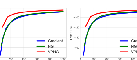
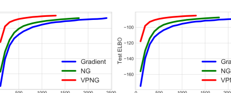
Figure 2: vae Learning curves on binarized MNIST

We compare the vpng method with the vanilla gradient and natural gradient optimizations. Since the traditional natural gradient does not deal with the model parameter ${\boldsymbol{\mathbf{\theta}}}$, we use the vanilla gradient for ${\boldsymbol{\mathbf{\theta}}}$ in this setting. We do not need to compare the performances of the vpng with the traditional natural gradient by fixing the model parameter ${\boldsymbol{\mathbf{\theta}}}$ and learning only the variational parameter ${\boldsymbol{\mathbf{\lambda}}}$ for two reasons. First, this setting is not common for vaes. Second, we need to have a fixed value for ${\boldsymbol{\mathbf{\theta}}}$ and it is difficult to obtain an optimal value for it before running the algorithms.

We select a batch size of 600 since we print the elbo values every 100 iterations. Hence, we evaluate the performances for each algorithm exactly once per epoch. The test elbo values are computed over the whole test set and the train elbo values are computed over a fixed set of 10,000 randomly-chosen (out of the whole 60,000) images. We allow each method to run for 1,000 seconds (we found similar results at longer runtimes) and select the best step sizes among several reasonable choices. Figure 2 shows the results. Though the vpng method is the slowest per iteration, it outperforms the baseline optimizations on both the train and test sets, even on running time. We also compare these methods with the second-order optimization method, the Hessian-free Stochastic Gaussian Variational Inference (HFSGVI) (Fan et al., 2015). However, it was not fast enough due to the large amount of Hessian-vector product computations. The elbo values with this method are still far below -200 within 1,000 seconds, which is much slower than the methods shown in Figure 2.

The intuitive reason for the performance gain stems from the fact that the vae parameters control pixels that are highly correlated across images. The vpng corrects for this correlation.

5.3 Variational matrix factorization

Our third experiment is on MovieLens 20M (Harper & Konstan, 2016). This is a movie recommendation dataset that contains 20 million movie ratings from $n\approx 135\text{K}$ users on $m_{\text{total}}\approx 27\text{K}$ movies. Each rating $R^{\text{raw}}_{u,i}$ of the movie $i$ by the user $u$ is a value in the set $\{0.5,1.0,1.5,\ldots,5.0\}$. We convert the ratings to integer values between 0 and 9 and select all movies with at least 5K ratings yielding $m\approx 1\text{K}$ movies. We model the zeros as in implicit matrix factorization (Gopalan et al., 2015). We use Poisson matrix factorization to model this data. Assume there is a latent representation ${\boldsymbol{\mathbf{\beta}}}_{u}\in\mathbb{R}^{d}$ for each user $u$ and there is a latent representation ${\boldsymbol{\mathbf{\theta}}}_{i}\in\mathbb{R}^{d}$ for each movie $i$. Here $d=100$ is the latent variable dimensionality. Denote $\text{softplus}(t)=\log(1+e^{t})$. We model the likelihood as

$$p(R\,|\,{\boldsymbol{\mathbf{\theta}}},{\boldsymbol{\mathbf{\beta}}})=\prod\limits_{u=1}^{n}\prod\limits_{i=1}^{m}\text{Poisson}(R_{u,i}\,|\,\mu=\text{softplus}({\boldsymbol{\mathbf{\beta}}}_{u}^{\top}{\boldsymbol{\mathbf{\theta}}}_{i})).$$

We do variational inference on the user latent variable ${\boldsymbol{\mathbf{\beta}}}$ and treat the movie variables ${\boldsymbol{\mathbf{\theta}}}$ as model parameters. The prior on each user latent variable is a standard Normal. We set the variational distribution as $q({\boldsymbol{\mathbf{\beta}}}\,|\,R;{\boldsymbol{\mathbf{\lambda}}})=\prod\limits_{u=1}^{n}q({\boldsymbol{\mathbf{\beta}}}_{u}\,|\,{\boldsymbol{\mathbf{R}}}_{u};{\boldsymbol{\mathbf{\lambda}}})$, where $q({\boldsymbol{\mathbf{\beta}}}_{u}\,|\,{\boldsymbol{\mathbf{R}}}_{u};{\boldsymbol{\mathbf{\lambda}}})$ uses an inference network that takes as input the row $u$ of the rating matrix $R$. Similar to the vae experiment, we use a 3-layer feed-forward neural network. We use 300 hidden units for this experiment.

Notice that the above likelihood is exactly a 1-layer feedforward neural network (without the bias term) that takes the latent representations drawn from the variational distribution $q({\boldsymbol{\mathbf{\beta}}}\,|\,R;{\boldsymbol{\mathbf{\lambda}}})$ and outputs the rating matrix as a random matrix with a pointwise Poisson likelihood. Hence, we could view the model as a single-layer generative network and treat the latent variable ${\boldsymbol{\mathbf{\theta}}}$ as its parameter. We have transformed variational matrix factorization to a task similar to the vae. Hence, when we apply Algorithm 1 to this model, we can apply the same tricks used in the vae experiments to accelerate the performances. We treat the whole model as a 4-layer feedforward neural network and again apply the tridiagonal block-wise K-FAC approximation (Martens & Grosse, 2015) and adopt low-rank approximations of large matrices (again, more details in appendix).

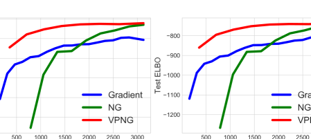
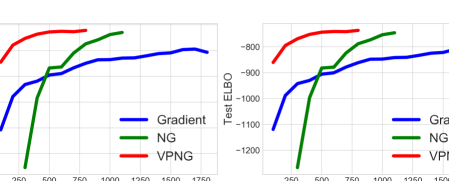
Figure 3: VMF Learning curves on MovieLens 20M

The results are shown in Figure 3. We randomly split the data matrix $R$ into train and test sets where the train set contains $90\%$ of the rows of $R$ (it contains ratings from $90\%$ of the users) and the test set contains the remaining rows. The test elbo values are computed over the random sampled test set and the train elbo values are computed over a fixed subset (with its size equal to the test set size) of the whole train set. Since this dataset is larger, we use a batch size of 3000. As can be seen in this figure, the vpng updates outperform the baseline optimizations on both the train and test learning curves. The curves look slightly different among various train/test splits of the dataset but Algorithm 1 consistently outperforms the baseline methods. The difference stems from the correlations in the ratings of the movies. The traditional natural gradient performs the worst at the beginning since it is only guaranteed to perform well at the end (when $q({\boldsymbol{\mathbf{z}}}\,|\,{\boldsymbol{\mathbf{x}}})$ is close to the posterior distribution $p({\boldsymbol{\mathbf{z}}}\,|\,{\boldsymbol{\mathbf{x}}})$, Equation 3 explains this), but not necessarily at the beginning, due to it does not consider potential curvature information in the model distribution. Across both experiments, we find that vpng dramatically improves estimation and inference at early iterations.

6 CONCLUSION

We introduced the variational predictive natural gradients. They adjust for parameter dependencies in variational inference induced by correlations in the observations. We show how to approximate the Fisher information without manual model-specific computations. We demonstrate the insight on a bivariate Gaussian model and the empirical value on a classification model on synthetic data, a deep generative model of images, and matrix factorization for movie recommendation. Future work includes extending to general Bayesian networks with multiple stochastic layers.

Appendix

We analyze the geometric structure of vpng to show its insight. Then we provide more details for the experiments.

Appendix A Analysis on the geometric structure of vpng

As discussed in Hoffman et al. (2013), the traditional natural gradient points to the steepest ascent direction of the elbo in the symmetric kl divergence space of the variational distribution $q$. Mathematically, for the elbo function as in Equation 1, the traditional natural gradient points to the direction of the solution to the following optimization problem, as $\epsilon\rightarrow 0$:

$$\operatorname*{arg\,max}_{\Delta{\boldsymbol{\mathbf{\lambda}}}} \ \ \ \ \mathcal{L}({\boldsymbol{\mathbf{\lambda}}}+\Delta{\boldsymbol{\mathbf{\lambda}}},{\boldsymbol{\mathbf{\theta}}})$$

s.t. $$\ \ \ \ \textrm{KL}_{\textrm{sym}}(q({\boldsymbol{\mathbf{\lambda}}})||q({\boldsymbol{\mathbf{\lambda}}}+\Delta{\boldsymbol{\mathbf{\lambda}}}))\leq\epsilon.$$

In fact, denote ${\boldsymbol{\mathbf{\eta}}}=\begin{pmatrix}{\boldsymbol{\mathbf{\lambda}}}\\ {\boldsymbol{\mathbf{\theta}}}\end{pmatrix}$, the reparameterization for ${\boldsymbol{\mathbf{z}}}=g({\boldsymbol{\mathbf{x}}},{\boldsymbol{\mathbf{\varepsilon}}};{\boldsymbol{\mathbf{\lambda}}})$ and $p_{{\boldsymbol{\mathbf{x}}}^{\prime}}({\boldsymbol{\mathbf{\eta}}})=p({\boldsymbol{\mathbf{x}}}^{\prime}\,|\,{\boldsymbol{\mathbf{z}}}=g({\boldsymbol{\mathbf{x}}},{\boldsymbol{\mathbf{\varepsilon}}};{\boldsymbol{\mathbf{\lambda}}});{\boldsymbol{\mathbf{\theta}}})$ to be the reparameterized predictive distribution, our vpng (as defined in Equation 14) shares similar geometric structures and points to the direction of the solution to the following optimization problem, as $\epsilon\rightarrow 0$:

$$\operatorname*{arg\,max}_{\Delta{\boldsymbol{\mathbf{\eta}}}} \ \ \ \ \mathcal{L}({\boldsymbol{\mathbf{\eta}}}+\Delta{\boldsymbol{\mathbf{\eta}}})$$ (18)

s.t. $$\ \ \ \ \mathbb{E}_{\boldsymbol{\mathbf{\varepsilon}}}\left[\textrm{KL}_{\textrm{sym}}(p_{{\boldsymbol{\mathbf{x}}}^{\prime}}({\boldsymbol{\mathbf{\eta}}})||p_{{\boldsymbol{\mathbf{x}}}^{\prime}}({\boldsymbol{\mathbf{\eta}}}+\Delta{\boldsymbol{\mathbf{\eta}}}))\right]\leq\epsilon.$$

Here the expectation on ${\boldsymbol{\mathbf{\varepsilon}}}$ takes with respect to the parameter-free distribution $s({\boldsymbol{\mathbf{\varepsilon}}})$ in the reparameterization.

Proof.

The proof for the above fact is similar with the proof for the traditional natural gradient as in Hoffman et al. (2013). Ideally, we want to find a (possibly approximate) Riemannian metric $G({\boldsymbol{\mathbf{\eta}}})$ to capture the geometric structure of the expected symmetric kl divergence $\mathbb{E}_{\boldsymbol{\mathbf{\varepsilon}}}\left[\text{KL}_{\text{sym}}(p_{{\boldsymbol{\mathbf{x}}}^{\prime}}({\boldsymbol{\mathbf{\eta}}})||p_{{\boldsymbol{\mathbf{x}}}^{\prime}}({\boldsymbol{\mathbf{\eta}}}+\Delta{\boldsymbol{\mathbf{\eta}}}))\right]$:

$$\mathbb{E}_{\boldsymbol{\mathbf{\varepsilon}}}\left[\text{KL}_{\text{sym}}(p_{{\boldsymbol{\mathbf{x}}}^{\prime}}({\boldsymbol{\mathbf{\eta}}})||p_{{\boldsymbol{\mathbf{x}}}^{\prime}}({\boldsymbol{\mathbf{\eta}}}+\Delta{\boldsymbol{\mathbf{\eta}}}))\right]\approx\Delta{\boldsymbol{\mathbf{\eta}}}^{\top}G({\boldsymbol{\mathbf{\eta}}})\Delta{\boldsymbol{\mathbf{\eta}}}$$

$$\ \ \ \ \ \ \ \ \ \ \ \ \ \ \ \ \ \ \ \ \ \ \ \ \ \ \ \ \ \ \ \ \ \ \ \ \ \ \ \ \ \ \ \ \ \ \ \ \ \ \ \ \ \ \ \ \ \ \ \ \ \ \ \ \ \ \ \ \ \ +o(\lVert\Delta{\boldsymbol{\mathbf{\eta}}}\rVert^{2}).$$

By making first-order Taylor approximation on $p_{{\boldsymbol{\mathbf{x}}}^{\prime}}({\boldsymbol{\mathbf{\eta}}}+\Delta{\boldsymbol{\mathbf{\eta}}})$ and $\log p_{{\boldsymbol{\mathbf{x}}}^{\prime}}({\boldsymbol{\mathbf{\eta}}}+\Delta{\boldsymbol{\mathbf{\eta}}})$, we get

$$\mathbb{E}_{\boldsymbol{\mathbf{\varepsilon}}}\left[\textrm{KL}_{\textrm{sym}}(p_{{\boldsymbol{\mathbf{x}}}^{\prime}}({\boldsymbol{\mathbf{\eta}}})||p_{{\boldsymbol{\mathbf{x}}}^{\prime}}({\boldsymbol{\mathbf{\eta}}}+\Delta{\boldsymbol{\mathbf{\eta}}}))\right]$$

$$= \mathbb{E}_{\boldsymbol{\mathbf{\varepsilon}}}[\int(p_{{\boldsymbol{\mathbf{x}}}^{\prime}}({\boldsymbol{\mathbf{\eta}}}+\Delta{\boldsymbol{\mathbf{\eta}}})-p_{{\boldsymbol{\mathbf{x}}}^{\prime}}({\boldsymbol{\mathbf{\eta}}}))$$

$$\ \ \ \ \ \ \ \ \ \ \ \ \cdot(\log p_{{\boldsymbol{\mathbf{x}}}^{\prime}}({\boldsymbol{\mathbf{\eta}}}+\Delta{\boldsymbol{\mathbf{\eta}}})-\log p_{{\boldsymbol{\mathbf{x}}}^{\prime}}({\boldsymbol{\mathbf{\eta}}}))d{\boldsymbol{\mathbf{x}}}^{\prime}]$$

$$= \mathbb{E}_{\boldsymbol{\mathbf{\varepsilon}}}[\int(\nabla_{\boldsymbol{\mathbf{\eta}}}p_{{\boldsymbol{\mathbf{x}}}^{\prime}}({\boldsymbol{\mathbf{\eta}}})^{\top}\Delta{\boldsymbol{\mathbf{\eta}}})\cdot(\nabla_{\boldsymbol{\mathbf{\eta}}}\log p_{{\boldsymbol{\mathbf{x}}}^{\prime}}({\boldsymbol{\mathbf{\eta}}})^{\top}\Delta{\boldsymbol{\mathbf{\eta}}})d{\boldsymbol{\mathbf{x}}}^{\prime}$$

$$\ \ \ \ \ \ \ \ \ \ \ \ +O(\lVert\Delta{\boldsymbol{\mathbf{\eta}}}\rVert^{3})]$$

$$= \mathbb{E}_{\boldsymbol{\mathbf{\varepsilon}}}[\int p_{{\boldsymbol{\mathbf{x}}}^{\prime}}({\boldsymbol{\mathbf{\eta}}})\cdot(\nabla_{\boldsymbol{\mathbf{\eta}}}\log p_{{\boldsymbol{\mathbf{x}}}^{\prime}}({\boldsymbol{\mathbf{\eta}}})^{\top}\Delta{\boldsymbol{\mathbf{\eta}}})$$

$$\ \ \ \ \ \ \ \ \ \ \ \ \cdot(\nabla_{\boldsymbol{\mathbf{\eta}}}\log p_{{\boldsymbol{\mathbf{x}}}^{\prime}}({\boldsymbol{\mathbf{\eta}}})^{\top}\Delta{\boldsymbol{\mathbf{\eta}}})d{\boldsymbol{\mathbf{x}}}^{\prime}+O(\lVert\Delta{\boldsymbol{\mathbf{\eta}}}\rVert^{3})]$$

$$= \Delta{\boldsymbol{\mathbf{\eta}}}^{\top}F_{r}\Delta{\boldsymbol{\mathbf{\eta}}}+O(\lVert\Delta{\boldsymbol{\mathbf{\eta}}}\rVert^{3}).$$

The term $O(\lVert\Delta{\boldsymbol{\mathbf{\eta}}}\rVert^{3})$ is negligible compared to the first term when $\epsilon\rightarrow 0$. Hence, we could take $G({\boldsymbol{\mathbf{\eta}}})$ to be just $F_{r}$, the variational predictive Fisher information as defined in Section 3.3. By Amari (1998)’s analysis on natural gradients, we know that the solution to Equation 18 points to the direction of $G({\boldsymbol{\mathbf{\eta}}})^{-1}\cdot\nabla_{{\boldsymbol{\mathbf{\lambda}}},{\boldsymbol{\mathbf{\theta}}}}\mathcal{L}=\nabla^{\lx@glossaries@gls@link{acronym}{VPNG}{\leavevmode\textsc{vpng}}}_{{\boldsymbol{\mathbf{\lambda}}},{\boldsymbol{\mathbf{\theta}}}}\mathcal{L}$, when $\epsilon\rightarrow 0$. ∎

Appendix B More details for the experiments

For the Bayesian Logistic regression experiment, we show the test AUC-iteration curve as in Figure 4. It can be seen that the vpng behaves more stable compared to the baseline methods.

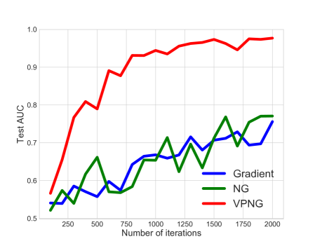
Figure 4: Bayesian Logistic regression test AUC-iteration learning curve.

For the vae and the vmf experiments, we chose hyperparameters for all methods based on the training elbo at the end of the time budget.

For the traditional natural gradient and vpng, we applied the dampening factor $\mu$. More precisely, we take vpng updates as $\hat{\nabla}_{{\boldsymbol{\mathbf{\theta}}},{\boldsymbol{\mathbf{\lambda}}}}^{\lx@glossaries@gls@link{acronym}{VPNG}{\leavevmode\textsc{vpng}}}\mathcal{L}~{}=~{}(\hat{F}_{r}+\mu I)^{-1}\cdot\nabla_{{\boldsymbol{\mathbf{\theta}}},{\boldsymbol{\mathbf{\lambda}}}}\mathcal{L}$ and traditional natural gradient updates as $\hat{\nabla}_{{\boldsymbol{\mathbf{\lambda}}}}^{\lx@glossaries@gls@link{acronym}{NG}{\leavevmode\textsc{ng}}}\mathcal{L}~{}=~{}(\hat{F}_{q}+\mu I)^{-1}\cdot\nabla_{{\boldsymbol{\mathbf{\lambda}}}}\mathcal{L}$). This is also applied in the Bayesian Logistic regression experiment in Section 5.1.

For the vae and the vmf experiments, we applied the K-FAC approximation (Martens & Grosse, 2015) to efficiently approximate the Fisher information matrices, in the ng and vpng computations. For the vpng s, we view the vae model as a 6-layer neural network and the vmf model as a 4-layer neural network. For the traditional ng s, we view both the vae model and the vmf model as 3-layer neural networks. We apply K-FAC on these models to efficiently approximate the Fisher information matrices with respect to the model distributions, given the samples from the variational distributions.

To apply the K-FAC approximation, we will need to compute matrix multiplications and matrix inversions for some non-diagonal large square matrices (i.e. the $\bar{A}_{0,0}$ matrices in the K-FAC paper (Martens & Grosse, 2015) and some other matrices that are computed during the K-FAC approximation process). In order to make the algorithms faster, we applied low-rank approximations for some large matrices of these forms by sparse eigenvalue decompositions. All of these large matrices are positive semi-definite. For each such large matrix $M$, we keep only the $K\cdot\ln(\text{dim}(M))$ dimensions of it with the largest eigenvalues and $K$ is a hyperparameter that can be tuned.

For ng and vpng, we applied the exponential moving averages for all matrices $\bar{A}_{i,i}$ and $\bar{G}_{i+1,i+1}$ (again, we use the notations in the K-FAC paper (Martens & Grosse, 2015)) to make the learning process more stable. We found that, by adding the exponential moving average technique, our vpng performs similarly to the case without this technique, while the traditional natural gradient is much more stable and efficient. If we do not apply the exponential moving average technique, the traditional natural gradients will not perform well. As an example, we show the performances of all methods without the exponential moving average technique in the vae experiment in Figure 5.

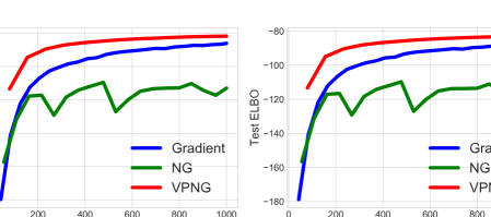
Figure 5: vae learning curves on binarized MNIST, without exponential moving averages

We found that ng and vpng performed similarly with respect to the dampening factor $\mu$, the exponential moving average decay parameter and the low-rank approximation function parameter $K$. However, different step sizes are needed to get the best performance from these two methods. We grid searched the step sizes and report the best one.

References

- Amari (1998) Amari, S.-I. Natural gradient works efficiently in learning. Neural computation, 10(2):251–276, 1998.
- Ba et al. (2016) Ba, J., Grosse, R., and Martens, J. Distributed second-order optimization using kronecker-factored approximations. 2016.
- Bowman et al. (2016) Bowman, S. R., Vilnis, L., Vinyals, O., Dai, A., Jozefowicz, R., and Bengio, S. Generating sentences from a continuous space. In Proceedings of The 20th SIGNLL Conference on Computational Natural Language Learning, pp. 10–21, 2016.
- Carbonetto et al. (2012) Carbonetto, P., Stephens, M., et al. Scalable variational inference for bayesian variable selection in regression, and its accuracy in genetic association studies. Bayesian analysis, 7(1):73–108, 2012.
- Fan et al. (2015) Fan, K., Wang, Z., Beck, J., Kwok, J., and Heller, K. A. Fast second order stochastic backpropagation for variational inference. In Advances in Neural Information Processing Systems, pp. 1387–1395, 2015.
- Gopalan et al. (2015) Gopalan, P., Hofman, J. M., and Blei, D. M. Scalable recommendation with hierarchical poisson factorization. In UAI, pp. 326–335, 2015.
- Grosse & Martens (2016) Grosse, R. and Martens, J. A kronecker-factored approximate fisher matrix for convolution layers. In International Conference on Machine Learning, pp. 573–582, 2016.
- Harper & Konstan (2016) Harper, F. M. and Konstan, J. A. The movielens datasets: History and context. ACM Transactions on Interactive Intelligent Systems (TiiS), 5(4):19, 2016.
- Harrison & Green (2010) Harrison, L. M. and Green, G. G. A bayesian spatiotemporal model for very large data sets. NeuroImage, 50(3):1126–1141, 2010.
- Hoffman et al. (2013) Hoffman, M., Blei, D., Wang, C., and Paisley, J. Stochastic variational inference. The Journal of Machine Learning Research, 14(1):1303–1347, 2013.
- Jordan et al. (1999) Jordan, M., Ghahramani, Z., Jaakkola, T., and Saul, L. An introduction to variational methods for graphical models. Machine learning, 37(2):183–233, 1999.
- Kingma & Welling (2014) Kingma, D. and Welling, M. Auto-encoding variational Bayes. In International Conference on Learning Representations, 2014.
- Kingma & Ba (2014) Kingma, D. P. and Ba, J. Adam: A method for stochastic optimization. arXiv preprint arXiv:1412.6980, 2014.
- LeCun et al. (1998) LeCun, Y., Bottou, L., Bengio, Y., and Haffner, P. Gradient-based learning applied to document recognition. Proceedings of the IEEE, 86(11):2278–2324, 1998.
- Liang et al. (2016) Liang, D., Charlin, L., McInerney, J., and Blei, D. M. Modeling user exposure in recommendation. In Proceedings of the 25th International Conference on World Wide Web, pp. 951–961. International World Wide Web Conferences Steering Committee, 2016.
- Manning et al. (2014) Manning, J. R., Ranganath, R., Norman, K. A., and Blei, D. M. Topographic factor analysis: a bayesian model for inferring brain networks from neural data. PloS one, 9(5):e94914, 2014.
- Martens & Grosse (2015) Martens, J. and Grosse, R. Optimizing neural networks with kronecker-factored approximate curvature. In International Conference on Machine Learning, pp. 2408–2417, 2015.
- Miao et al. (2016) Miao, Y., Yu, L., and Blunsom, P. Neural variational inference for text processing. In International Conference on Machine Learning, pp. 1727–1736, 2016.
- Mnih & Gregor (2014) Mnih, A. and Gregor, K. Neural variational inference and learning in belief networks. arXiv preprint arXiv:1402.0030, 2014.
- Mnih & Salakhutdinov (2008) Mnih, A. and Salakhutdinov, R. R. Probabilistic matrix factorization. In Advances in neural information processing systems, pp. 1257–1264, 2008.
- Ollivier et al. (2011) Ollivier, Y., Arnold, L., Auger, A., and Hansen, N. Information-geometric optimization algorithms: A unifying picture via invariance principles. arXiv preprint arXiv:1106.3708, 2011.
- Ranganath et al. (2014) Ranganath, R., Gerrish, S., and Blei, D. Black box variational inference. In Artificial Intelligence and Statistics, pp. 814–822, 2014.
- Ranganath et al. (2016) Ranganath, R., Perotte, A., Elhadad, N., and Blei, D. Deep survival analysis. In Machine Learning for Healthcare Conference, pp. 101–114, 2016.
- Regier et al. (2017) Regier, J., Jordan, M. I., and McAuliffe, J. Fast black-box variational inference through stochastic trust-region optimization. In Advances in Neural Information Processing Systems, pp. 2399–2408, 2017.
- Rezende et al. (2014) Rezende, D., Mohamed, S., and Wierstra, D. Stochastic backpropagation and approximate inference in deep generative models. In International Conference on Machine Learning, pp. 1278–1286, 2014.
- Shi et al. (2014) Shi, T., Tang, D., Xu, L., and Moscibroda, T. Correlated compressive sensing for networked data. In UAI, pp. 722–731, 2014.
- Stegle et al. (2010) Stegle, O., Parts, L., Durbin, R., and Winn, J. A bayesian framework to account for complex non-genetic factors in gene expression levels greatly increases power in eqtl studies. PLoS computational biology, 6(5):e1000770, 2010.
- Thomas et al. (2016) Thomas, P., Silva, B. C., Dann, C., and Brunskill, E. Energetic natural gradient descent. In International Conference on Machine Learning, pp. 2887–2895, 2016.
- Tieleman & Hinton (2012) Tieleman, T. and Hinton, G. Lecture 6.5-rmsprop: Divide the gradient by a running average of its recent magnitude. COURSERA: Neural networks for machine learning, 4(2):26–31, 2012.
- Titsias & Lázaro-Gredilla (2014) Titsias, M. and Lázaro-Gredilla, M. Doubly stochastic variational bayes for non-conjugate inference. In International Conference on Machine Learning, pp. 1971–1979, 2014.