h Cavendish-HEP-19/04
A new type of charged black hole bomb

Abstract

Black hole bombs are usually constructed by surrounding an ergoregion by a mirror. The fields propagating between the event horizon and the mirror are prevented from escaping to infinity and reflected back to the ergoregion, thus undergoing repeated superradiant scattering which leads to a linear instability. We introduce a new construction in which the field is outside the mirror and is therefore prevented from falling into the black hole but is free to escape to infinity. Provided the mirror is inside the ergoregion, it turns out that this still causes linear instabilities. This behaviour is observed on Reissner-Nordstr m and de Sitter-Reissner-Nordstr m backgrounds using numerical simulations, based on a semi-implicit discretisation on a first-order system formulation of the partial differential equations governing the evolution of the scalar field. We also perform simulations for a standard black hole bomb and for another type of contraption: a sandwich black hole bomb.

1 Introduction

In 1969, R. Penrose [21] noticed the possibility of extracting rotational energy from a rotating black hole using test particles or material objects. In a Gedankenexperiment now known as the Penrose process, a test particle is sent from infinity into the ergoregion, where it splits in two particles. The first one is directed in such a manner that it has negative energy as measured by an observer static at infinity. It cannot escape, because its energy is conserved and negative energy is only possible inside the ergoregion. Eventually, it falls through the event horizon. The other particle is free to escape to infinity and since the total energy is conserved, its energy is positive and larger than that of the particle that was originally sent in. The analogue of the Penrose process for fields is referred to as superradiance. It is a scattering process with a reflection coefficient that is larger than $1$. In black hole spacetimes, superradiance can be caused by rotation, as first observed by Zeldovich in 1971 and 1972 [26, 27], or by the interaction of the charges of the field and the black hole. In the first case, the phenomenon is localised in a fixed geometrical region outside the black hole, called the ergoregion and determined uniquely in terms of the mass, charge, and angular momentum of the black hole as well as the cosmological constant. In the second case, the ergoregion depends on both the physical parameters of the black hole and the field and in some situations may cover the whole exterior of the black hole.

Rotational superradiance has been investigated more thoroughly than the charge induced one, probably because of its greater physical significance, since one expects stellar objects to be electrically neutral. The charged case is nevertheless interesting, albeit on a more abstract level, because of its very distinct analytical and geometrical features. In particular, it may be a harder problem in terms of analysis of partial differential equations than the rotational case, which is solved at least partially for the Kerr and Kerr-de Sitter families, whereas even the spherically symmetric situation is not well understood for charge induced superradiance. For a long time, as far as we are aware, there was only one analytical study available in the literature, due to A. Bachelot [1]. This remarkable work essentially gives a complete description of the spherically symmetric case. It notably characterises the situations giving rise to the extraction of an infinite amount of energy by a simple analytic property of the radial speed of the radial null geodesics, but this property is difficult to verify in black hole spacetimes and the finiteness of the reflection coefficient is still an open question. Recently, N. Besset [2] proved the decay of the local energy of charged Klein-Gordon fields outside a subextremal de Sitter-Reissner-Nordstr m black hole, using a resonance expansion of the propagator.

The numerical investigations of the charged case are very scarce and were mostly done in the frequency domain. A study in the time domain was published by two of the authors (LDM and JPN [10]) where a spontaneous behaviour, very similar to the Penrose process, was observed numerically for charged scalar fields outside a Reissner-Nordstrøm black hole: a wave packet is sent from outside the ergoregion towards the horizon. As it enters the ergoregion, it splits spontaneously into an incoming wave packet with negative energy, which falls into the black hole and, an outgoing wave packet, with positive energy larger than that of the initial incoming one, which propagates to infinity. Another type of superradiant behaviour was also observed in Ref. [10], associated with so-called flare initial data. These are a class of initial data supported within the ergoregion but on which the energy is positive definite (the data for the field is zero and the data for its time derivative is a gaussian multiplied by an oscillatory exponential). The energy gains obtained for flare data are much larger than for incoming wave packets and far exceed the theoretical limits for scattering experiments, given by reflection coefficients. Similar initial data were studied by methods of geometric optics by G. Eskin in Ref. [11]. For a comprehensive list of references on superradiance and a thorough investigation of the phenomenon in its many aspects, see the book Superradiance by R. Brito, V. Cardoso, and P. Pani [4].

The concept of a black hole bomb was originally proposed in 1972 by W. H. Press and S. A. Teukolsky [22, 23]. A spherical mirror is constructed around a Kerr black hole, in the exterior region. A scalar field propagating outside the black hole and inside the mirror is thus prevented from escaping to infinity and undergoes repeated superradiant scattering inside the ergoregion. The result is a linear instability, i.e. an exponential growth of the amplitude of the field. Since it is usual to set reflecting boundary conditions at the timelike conformal boundary of anti-de Sitter spacetime, asymptotically anti-de Sitter black holes provide a realisation of a black hole bomb without the need to construct a mirror, and has been the subject of numerous studies, see for example H. Witek, V. Cardoso, C. Herdeiro, A. Nerozzi, U. Sperhake and M. Zilh o [25], S. Green, S. Hollands, A. Ishibashi and R. Wald [13] and references therein and also the recent numerical study of the fully coupled Einstein-charged scalar field system by P.M. Chesler and D.A. Lowe [6]. A similar construction to the one proposed in Ref. [22] can be performed outside a charged black hole. These charged black hole bombs have been somewhat less investigated than their rotating analogues but there is still a fair amount of studies, mostly numerical, available in the literature, for instance Ref. [4, 8, 9, 14, 17, 18].

In this article, we propose a new type of black hole bomb in which the field is located outside the mirror. Our numerical simulations show that provided the mirror is located inside the ergoregion, this still leads to a linear instability. Although the field is free to escape the ergoregion, we observe that a part of the solution with negative energy creeps along the mirror and sends out repeated bursts of positive energy while its amplitude increases exponentially. For completeness, we also study the more classic black hole bombs and another new type of bomb, the sandwich bomb, for which one naturally anticipates linear instability. The simulations in these cases give the expected results and provide a validation of our numerical scheme. We use the following terminology for our different versions of the bombs:

• classic, or type I, charged black hole bomb; it is analogous to the Press-Teukolsky bomb; the field propagates between the mirror and the horizon;

• type II charged black hole bomb; this time the mirror is set within the ergoregion and the field propagates outside of the mirror;

• type III, or sandwich, charged black hole bomb; the field is sandwiched between two mirrors, the innermost one being set inside the ergoregion.

The simulations are performed in the time domain for charged scalar fields in the exterior of a subextremal Reissner-Nordstr m or de Sitter-Reissner-Nordstr m black hole. The initial data are of flare-type and are supported inside the ergoregion.

The article is organised as follows. Section 2 is devoted to a brief presentation of de Sitter-Reisser-Nordstr m and Reissner-Nordstr m metrics and of the charged Klein-Gordon equation on such backgrounds. The three types of black hole bombs are described in Section 3. We describe in Section 4 the numerical method that is used for the simulations, with particular attention paid on the energy conservation at a discrete level. Finally, the numerical simulations of black hole bombs for types I, II, and III, are presented and discussed in Section 5.

2 Geometrical and analytical framework

2.1 Reissner-Nordstr m and de Sitter-Reissner-Nordstr m metrics

The de Sitter-Reissner-Nordstr m metric is a $3$-parameter family of solutions of the Einstein-Maxwell equations with positive cosmological constant. In Schwarzschild coordinates $(t,r,\omega)\in\mathbb{R}\times]0,+\infty[\times S^{2}$, it has the following expression:

$$g=F(r)\mathrm{d}t^{2}-F(r)^{-1}\mathrm{d}r^{2}-r^{2}\mathrm{d}\omega^{2}\,,$$ (1)

with $\mathrm{d}\omega^{2}$ the euclidean metric on $\mathbb{S}^{2}$,

$$F(r)=1-\frac{2M}{r}+\frac{Q^{2}}{r^{2}}-\Lambda r^{2}\,,$$

$M$ being the mass of the black hole, $Q$ its charge, and $\Lambda>0$ the cosmological constant.

Setting $\Lambda=0$, we recover the Reissner-Nordstr m solution while the de Sitter-Schwarzschild family corresponds to $Q=0$. We also obtain the Schwarzschild metric for $Q=0$, $\Lambda=0$ and Minkowski spacetime when all three parameters $M,Q,\Lambda$ are zero.

The zeros of the function $F$ on the positive real axis correspond to event horizons. Note that

$$F(r)=\frac{-\Lambda r^{4}+r^{2}-2Mr+Q^{2}}{r^{2}}$$

and the coefficient of the term in $r^{3}$ in the numerator is zero. Hence, the sum of the roots of $F$ counted with their multiplicity is zero. It follows that there are at most three event horizons. The subextremal case corresponds to the presence of exactly three event horizons. In this case, the function $F$ has one negative zero and three distinct positive ones: $r_{n}<0<r_{-}<r_{0}<r_{+}$, with $r_{n}=-(r_{-}+r_{0}+r_{+})$. The innermost horizon $\{r=r_{-}\}$ is the Cauchy horizon, $\{r=r_{0}\}$ is referred to as the horizon of the black hole, and $\{r=r_{+}\}$ is the cosmological horizon. The spacetime is made of four distinct regions separated by the horizons:

• Block I is the region beyond the inner horizon ($0<r<r_{-}$); it is a static region containing a timelike curvature singularity at $r=0$;

• Block II is the part of spacetime between the black hole and the Cauchy horizons ($r_{-}<r<r_{0}$); it is a dynamic region, $\partial_{t}$ is spacelike;

• Block III is between the black hole and the cosmological horizons ($r_{0}<r<r_{+}$); we refer to it as the exterior of the black hole; it is static;

• Block IV is the dynamic region beyond the cosmological horizon ($r>r_{+}$).

Due to the rather large number of horizons which are all bifurcate, the construction of the maximal analytic extension of the subextremal de Sitter-Reissner-Nordstr m spacetime is intricate. For a clear and thorough description of it, we refer the reader to the recent detailed study by M. Mokdad [20]. The extreme cases correspond to double or triple horizons. There are three distinct extreme cases corresponding to $r_{n}<0<r_{-}=r_{0}<r_{+}$, $r_{n}<0<r_{-}<r_{0}=r_{+}$, and $r_{n}<0<r_{-}=r_{0}=r_{+}$. Precise conditions on the parameters $M$, $Q$, and $\Lambda$ characterising the subextremal, extreme, and superextremal (no horizon) cases will be derived in a subsequent work.

For $\Lambda=0$, the function $F$ simplifies to

$$F(r)=1-\frac{2M}{r}+\frac{Q^{2}}{r^{2}}$$

and the conditions for extremality, subextremality, and superextremality are easily obtained.

1. Subextremal case: for $M>|Q|$, the function $F$ has two real roots

   $$r_{-}=M-\sqrt{M^{2}-Q^{2}}\,,~{}r_{0}=M+\sqrt{M^{2}-Q^{2}}\,,$$ (2)

   corresponding to the Cauchy horizon $\{r=r_{-}\}$ and the outer horizon, or horizon of the black hole, $\{r=r_{0}\}$. The spacetime is made of three blocks

   $${\cal B}_{\mbox{\tiny I}}=\{0<r<r_{-}\}\,,~{}{\cal B}_{\mbox{\tiny II}}=\{r_{-}<r<r_{0}\}\,,~{}{\cal B}_{\mbox{\tiny III}}=\{r_{0}<r\}\,.$$

2. Extreme case: for $M=|Q|$, $r_{0}=r_{-}=M$ is the only root of $F$ and there is only one horizon. Block II is no longer there and the spacetime is made of blocks I and III.

3. Superextremal case: for $M<|Q|$, the function $F$ has no real root. There are no horizons, the space-time contains no black hole and the singularity $\{r=0\}$ is naked (i.e. not hidden beyond a horizon).

2.1.1 The Regge-Wheeler coordinate

The Regge-Wheeler coordinate is a function $r_{*}$ of $r$ such that

$$\frac{{\mathrm{d}}r_{*}}{{\mathrm{d}}r}=\frac{1}{F(r)}.$$ (3)

Expressed in coordinates $(t,r_{*},\omega)$, the radial null geodesics, which are also the principal null geodesics (their tangent vectors are double roots of the Weyl tensor), are described as the straight lines

$$t=\pm r_{*}+C\,,~{}C\in\mathbb{R}\,.$$

Moreover the metric $g$ takes the form:

$$g=F(r)({\mathrm{d}}t^{2}-{\mathrm{d}}r^{2}_{*})-r^{2}{\mathrm{d}}\omega^{2}.$$ (4)

Let us give a more precise description of $r_{*}$ in the situations we mean to study.

• In the subextremal de Sitter-Reissner-Nordstr m case, the function $F$ can be written as:

  $$F(r)=-\Lambda\frac{(r-r_{n})(r-r_{-})(r-r_{0})(r-r_{+})}{r^{2}},$$

  with $r_{n}<0<r_{-}<r_{0}<r_{+}$. The variable $r_{*}$ is given by

  $$r_{*}=\frac{1}{\kappa_{n}}\log|r-r_{n}|+\frac{1}{\kappa_{-}}\log|r-r_{-}|+\frac{1}{\kappa_{0}}\log|r-r_{0}|+\frac{1}{\kappa_{+}}\log|r-r_{+}|+R_{0}\,,$$ (5)

  where

  $$\kappa_{n}=F^{\prime}(r_{n}) = -\Lambda\frac{(r_{n}-r_{-})(r_{n}-r_{0})(r_{n}-r_{+})}{r_{n}^{2}}>0\,,$$

  $$\kappa_{-}=F^{\prime}(r_{-}) = -\Lambda\frac{(r_{-}-r_{n})(r_{-}-r_{0})(r_{-}-r_{+})}{r_{-}^{2}}<0\,,$$

  $$\kappa_{0}=F^{\prime}(r_{0}) = -\Lambda\frac{(r_{0}-r_{n})(r_{0}-r_{-})(r_{0}-r_{+})}{r_{0}^{2}}>0\,,$$

  $$\kappa_{+}=F^{\prime}(r_{+}) = -\Lambda\frac{(r_{+}-r_{n})(r_{+}-r_{-})(r_{+}-r_{0})}{r_{+}^{2}}<0$$

  and $R_{0}$ is a constant of integration. We see that in block III, as $r\rightarrow r_{0}$, $r_{*}\rightarrow-\infty$ and as $r\rightarrow r_{+}$, $r_{*}\rightarrow+\infty$; $r_{*}$ is an analytic diffeomorphism from $]r_{0},r_{+}[$ onto $\mathbb{R}$ and ${\cal B}_{\mbox{\tiny III}}$ is described in $(t,r_{*},\omega)$ coordinates by

  $${\cal B}_{\mbox{\tiny III}}=\mathbb{R}_{t}\times\Sigma\,,~{}\Sigma=\mathbb{R}_{r_{*}}\times\mathbb{S}^{2}_{\omega}\,.$$

  Moreover,

  $$r-r_{0}\simeq e^{\kappa_{0}r_{*}}\mbox{ as }r_{*}\rightarrow-\infty\,;~{}r_{+}-r\simeq e^{\kappa_{+}r_{*}}\mbox{ as }r_{*}\rightarrow+\infty\,.$$

• In the subextremal Reissner-Nordstr m situation,

  $$F(r)=\frac{r^{2}-2Mr+Q^{2}}{r^{2}}=\frac{(r-r_{-})(r-r_{0})}{r^{2}}$$

  and we have

  $$r_{*}=r+\frac{1}{\kappa_{-}}\log|r-r_{-}|+\frac{1}{\kappa_{0}}\log|r-r_{0}|+R_{0}\,,$$ (6)

  with

  $$\kappa_{-}=F^{\prime}(r_{-})=\frac{r_{-}-r_{0}}{r_{-}^{2}}<0\,,~{}\kappa_{0}=F^{\prime}(r_{0})=\frac{r_{0}-r_{-}}{r_{0}^{2}}>0,$$

  and $R_{0}$ a constant of integration. In ${\cal B}_{\mbox{\tiny III}}$, as $r\rightarrow r_{0}$, $r_{*}$ tends to $-\infty$ and as $r\rightarrow+\infty$, $r_{*}\rightarrow+\infty$; $r_{*}$ is an analytic diffeomorphism from $]r_{0},+\infty[$ onto $\mathbb{R}$ and ${\cal B}_{\mbox{\tiny III}}$ is described in $(t,r_{*},\omega)$ coordinates by

  $${\cal B}_{\mbox{\tiny III}}=\mathbb{R}_{t}\times\Sigma\,,~{}\Sigma=\mathbb{R}_{r_{*}}\times\mathbb{S}^{2}_{\omega}\,.$$

  Moreover,

  $$r-r_{0}\simeq e^{\kappa_{0}r_{*}}\mbox{ as }r_{*}\rightarrow-\infty\,;~{}r\simeq r_{*}\mbox{ as }r_{*}\rightarrow+\infty\,.$$

2.2 Charged Klein-Gordon equation, conserved energy current and ergoregion

In the present article, we shall focus on the evolution of charged scalar fields, in block III of subextremal Reissner-Nordstr m and de Sitter-Reissner-Nordstr m black holes, seen by an observer whose perception of time is described by the variable $t$. Such observers are completely natural in asymptotically flat situations since they are the analytic continuation inside the spacetime of static observers at infinity. In an asymptotically de Sitter universe, there is no such interpretation. In the cases we consider however, they are natural for a different reason, which is equally valid in the asymptotically flat and asymptotically de Sitter cases: they are associated with the only future-oriented timelike Killing vector field in block III that is orthogonal to a family of spacelike slices ($\partial_{t}$ in Schwarzschild coordinates).

The charged Klein-Gordon equation on our backgrounds is given by

$$\Box^{A}_{g}f+m^{2}f=0\,,~{}\Box^{A}_{g}f=(\nabla_{a}-iqA_{a})(\nabla^{a}-iqA^{a}),$$ (7)

where $A$ is the electromagnetic potential $1$-form of the spacetime, given by

$$A_{a}{\mathrm{d}}x^{a}=\frac{Q}{r}{\mathrm{d}}t\,.$$

Then, (7) can be explicitly written as

$$\left[\frac{1}{F}\left(\frac{\partial}{\partial t}-i\frac{qQ}{r}\right)^{2}-\frac{1}{r^{2}}\frac{\partial}{\partial r}r^{2}F\frac{\partial}{\partial r}-\frac{1}{r^{2}}\Delta_{S^{2}}+m^{2}\right]f=0,$$ (8)

with $\Delta_{S^{2}}$ the Laplace-Beltrami operator on $\mathbb{S}^{2}$. Putting $\phi=rf$ and using the Regge-Wheeler coordinate $r_{*}$ defined above, (8) has the following expression:

$$\left(\partial^{2}_{t}-\partial^{2}_{r_{*}}\right)\phi-2i\frac{qQ}{r}\partial_{t}\phi+F(r)\left[\frac{-\Delta_{S^{2}}\phi}{r^{2}}+m^{2}\phi+\frac{F^{\prime}(r)}{r}\phi\right]-\frac{q^{2}Q^{2}}{r^{2}}\phi=0\,.$$ (9)

As was observed in Ref. [10], (7) admits a conserved energy current which can be obtained from a non conserved stress-energy tensor. Indeed, (7) is not covariant in the sense that it is not coupled back to the Maxwell equations. This means that there is no natural conserved stress-energy tensor for (7). But we can introduce in the stress-energy tensor for the uncharged Klein-Gordon equation a natural modification involving the electromagnetic potential. Putting

$$T_{ab}=\sum_{j=1}^{2}\left(\partial_{a}f_{j}\partial_{b}f_{j}-\frac{1}{2}g^{cd}\left(\partial_{c}f_{j}\partial_{d}f_{j}+q^{2}A_{c}A_{d}\left(f_{j}\right)^{2}\right)g_{ab}+\frac{m^{2}}{2}(f_{j})^{2}g_{ab}\right)\,,$$ (10)

where $f_{1}=\Re f$ and $f_{2}=\Im f$. We construct an energy current by contracting $T_{ab}$ with $\partial_{t}$

$$J^{a}\partial_{a}:=T_{0}^{a}\partial_{a} = \sum_{j=1}^{2}\left(\partial_{t}f_{j}\nabla f_{j}+\frac{1}{2}\left[-\langle\nabla f_{j},\nabla f_{j}\rangle_{g}-q^{2}\langle A,A\rangle_{g}f_{j}^{2}+m^{2}f_{j}^{2}\right]\partial_{t}\right)$$ (11)

$$= \sum_{j=1}^{2}\left(\partial_{t}f_{j}\nabla f_{j}+\frac{1}{2}\left[-\langle\nabla f_{j},\nabla f_{j}\rangle_{g}+(m^{2}-F^{-1}\frac{q^{2}Q^{2}}{r^{2}})f_{j}^{2}\right]\partial_{t}\right)\,.$$

It was established in Ref. [10] that, although $\nabla^{a}T_{ab}\neq 0$, we have $\nabla^{a}J_{a}=0$ for any solution $f$ of Ref. (7) (the proof in Ref. [10] was written for the Reissner-Nordstr m case but it extends without modification to the de Sitter-Reissner-Nordstr m framework).

The energy flux across a hypersurface

$$\Sigma_{t}:=\{t\}\times\mathbb{R}_{r_{*}}\times\mathbb{S}^{2}\,,$$

is given by (see Ref. [10] for details)

$${\cal F}_{\Sigma_{t}} = \frac{1}{2}\int_{\Sigma_{t}}\left(|\partial_{t}f|^{2}+|\partial_{r_{*}}f|^{2}+\frac{F}{r^{2}}|\nabla_{S^{2}}f|^{2}\right.$$ (12)

$$\hskip 36.135pt\left.+\left(Fm^{2}-\frac{q^{2}Q^{2}}{r^{2}}\right)|f|^{2}\right)r^{2}\mathrm{d}r_{*}\mathrm{d}^{2}\omega$$

$$= \frac{1}{2}\int_{\Sigma_{t}}\left(|\partial_{t}\phi|^{2}+|\partial_{r_{*}}\phi|^{2}+\frac{F}{r^{2}}|\nabla_{S^{2}}\phi|^{2}\right.$$

$$\hskip 36.135pt\left.+\left(\frac{FF^{\prime}}{r}+Fm^{2}-\frac{q^{2}Q^{2}}{r^{2}}\right)|\phi|^{2}\right)\mathrm{d}r_{*}\mathrm{d}^{2}\omega\,,$$

where

$$|\nabla_{S^{2}}f|^{2}=|\partial_{\theta}f|^{2}+\frac{1}{\sin^{2}\theta}|\partial_{\varphi}f|^{2}\mbox{ and }\mathrm{d}^{2}\omega=\sin\theta\mathrm{d}\theta\mathrm{d}\varphi\,.$$

Across a hypersurface

$$[t_{1},t_{2}]\times S_{R}\,,~{}S_{R}=\{R\}_{r_{*}}\times\mathbb{S}^{2}_{\omega}\,,$$

the outgoing energy flux has the form

$${\cal F}_{[t_{1},t_{2}]\times S_{R}} = \int_{[t_{1},t_{2}]\times S_{R}}\left(-\partial_{t}f_{1}\partial_{r_{*}}f_{1}-\partial_{t}f_{2}\partial_{r_{*}}f_{2}\right)r^{2}\mathrm{d}t\mathrm{d}^{2}\omega$$ (13)

$$= -\sum_{j=1}^{2}\int_{[t_{1},t_{2}]\times S_{R}}\partial_{t}\phi_{j}\left(\partial_{r_{*}}\phi_{j}-\frac{F}{r}\phi_{j}\right)\mathrm{d}t\mathrm{d}^{2}\omega\,.$$

If we consider a solution of (7) with given angular momentum $l(l+1)$, $l\in\mathbb{N}$, i.e. such that $-\Delta_{{\mathbb{S}}^{2}}f=l(l+1)f$, or equivalently $-\Delta_{{\mathbb{S}}^{2}}\phi=l(l+1)\phi$, we have

$${\cal F}_{\Sigma_{t}}=\frac{1}{2}\int_{\Sigma_{t}}\left(|\partial_{t}\phi|^{2}+|\partial_{r_{*}}\phi|^{2}+\left(F\frac{l(l+1)}{r^{2}}+\frac{FF^{\prime}}{r}+Fm^{2}-\frac{q^{2}Q^{2}}{r^{2}}\right)|\phi|^{2}\right)\mathrm{d}r_{*}\mathrm{d}^{2}\omega\,.$$ (14)

Denoting

$$P=F\frac{l(l+1)}{r^{2}}+\frac{FF^{\prime}}{r}+Fm^{2}\,,~{}V=\frac{qQ}{r}\,,$$ (15)

the potential $P-V^{2}$ appearing in (14) becomes negative as $r_{*}\rightarrow-\infty$ in the Reissner-Nordstr m case and as $r_{*}\rightarrow\pm\infty$ in the de Sitter-Reissner-Nordstr m case.

Definition 2.1 (Ergoregion).

The ergoregion $\cal E$ is the region where the energy density in (12) is allowed to become negative. For a fixed angular momentum $l\in\mathbb{N}$, this is exactly the region where $P$ is negative.

We see that in the Reissner-Nordstr m situation, $\cal E$ contains a domain of the form

$$\mathbb{R}_{t}\times]-\infty,R[_{r_{*}}\times\mathbb{S}^{2}\,,~{}R\in\mathbb{R}\,,$$

while in the de Sitter-Reissner-Nordstr m case, $\cal E$ contains a domain of the form

$$\mathbb{R}_{t}\times\left(]-\infty,R_{1}[_{r_{*}}\cup]R_{2},+\infty[_{r_{*}}\right)\times\mathbb{S}^{2}\,,~{}-\infty<R_{1}<R_{2}<+\infty\,.$$

Remark 2.1.

The ergoregion could also be defined as the region where the energy density on $\Sigma_{t}$ expressed in terms of $f$ is allowed to become negative. In this case it would be characterised for a given angular momentum $l$ as the region where

$$F\frac{l(l+1)}{r^{2}}+Fm^{2}-\frac{q^{2}Q^{2}}{r^{2}}<0\,.$$

The two definitions are not equivalent but the property immediately above is valid for both.

3 Black hole bombs

The three models of black hole bombs that we discuss in this article are constructed by setting spherical mirrors outside a subextremal Reissner-Nordstr m or de Sitter-Reissner-Nordstr m black hole. A mirror is simply described in the evolution system as a homogeneous Neumann (resp. Dirichlet) boundary condition, i.e. the normal derivative of the field (resp. the field) is set to zero at the surface of the mirror. These two conditions are commonly used when dealing with partial differential equations set on bounded domains. As it will be seen below, they lead to different properties for the corresponding solutions.

We describe each type of bomb with boundary conditions involving an abstract boundary operator $B$: Dirichlet conditions correspond to $Bu=u$ and Neumann conditions to $Bu=\partial_{r_{*}}u$. We set at $t=0$ some flare type data, entirely contained inside the ergoregion. Let $R\in\mathbb{R}$ such that $\mathbb{R}_{t}\times]-\infty,R[_{r_{*}}\times\mathbb{S}^{2}\subset{\cal E}$.

• Type I bombs. They are directly inspired by the Press-Teukolsky construction [22]. The mirror may surround the whole ergoregion or only a part of it and the field evolves beneath the mirror outside the black hole. See Figure 1 on the left. Let $R_{1}\in\mathbb{R}$, not necessarily lower than $R$, we set the mirror on the hypersurface $\{r_{*}=R_{1}\}$ and we study the boundary initial value problem:

  $$\left\{\begin{array}[]{l}{\phi\mathrm{~{}solution~{}of~{}}\eqref{CKG3}\mathrm{~{}on~{}}\mathbb{R}^{+}_{t}\times]-\infty,R_{1}[_{r_{*}}\times\mathbb{S}^{2}_{\omega}\,,}\\ {B\phi|_{r_{*}=R_{1}}=0\,,~{}\forall\,t\geq 0\,,}\\ {\phi|_{t=0}=0\,,~{}\partial_{t}\phi|_{t=0}=\phi_{1}\in{\cal C}^{\infty}_{c}(]-\infty,\min\{R,R_{1}\}[_{r_{*}}\times\mathbb{S}^{2}_{\omega})\,,}\end{array}\right.$$ (16)

  where ${\cal C}^{\infty}_{c}(\Omega)$ denotes the space of smooth functions on $\Omega$ whose support is a compact subset of $\Omega$.

• Type II bombs. The mirror is set within the ergoregion so that a part of $\cal E$ lies outside of it. The field propagates outside of the mirror. See Figure 1 in the centre. Precisely, let $R_{1}\in]-\infty,R[$, we set the mirror on the hypersurface $\{r_{*}=R_{1}\}$ and we study the boundary initial value problem:

  $$\left\{\begin{array}[]{l}{\phi\mathrm{~{}solution~{}of~{}}\eqref{CKG3}\mathrm{~{}on~{}}\mathbb{R}^{+}_{t}\times]R_{1},+\infty[_{r_{*}}\times\mathbb{S}^{2}_{\omega}\,,}\\ {B\phi|_{r_{*}=R_{1}}=0\,,~{}\forall\,t\geq 0\,,}\\ {\phi|_{t=0}=0\,,~{}\partial_{t}\phi|_{t=0}=\phi_{1}\in{\cal C}^{\infty}_{c}(]R_{1},R[_{r_{*}}\times\mathbb{S}^{2}_{\omega})\,.}\end{array}\right.$$ (17)

• Type III bombs. There are two mirrors, the inner one being set inside the ergoregion, the outer one may be set inside or outside of the ergoregion. The field propagates between the two mirrors. See Figure 1 on the right. Let $-\infty<R_{1}<R_{2}<+\infty$ with $R_{1}<R$. The mirrors are set on the hypersurfaces $\{r_{*}=R_{1}\}$ and $\{r_{*}=R_{2}\}$ and we study the boundary initial value problem:

  $$\left\{\begin{array}[]{l}{\phi\mathrm{~{}solution~{}of~{}}\eqref{CKG3}\mathrm{~{}on~{}}\mathbb{R}^{+}_{t}\times]R_{1},R_{2}[_{r_{*}}\times\mathbb{S}^{2}_{\omega}\,,}\\ {B\phi|_{r_{*}=R_{1}}=0\,,~{}B\phi|_{r_{*}=R_{2}}=0\,,~{}\forall\,t\geq 0\,,}\\ {\phi|_{t=0}=0\,,~{}\partial_{t}\phi|_{t=0}=\phi_{1}\in{\cal C}^{\infty}_{c}(]R_{1},\min\{R,R_{2}\}[_{r_{*}}\times\mathbb{S}^{2}_{\omega})\,.}\end{array}\right.$$ (18)

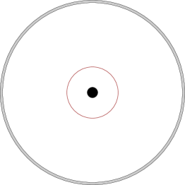
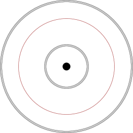
Figure 1: The three models of black hole bombs: types I, II, and III from left to right. The black disc is the black hole horizon and what is beyond, the red circle is the outer boundary of the ergoregion and mirrors are represented as thick grey circles.

By general theorems for hyperbolic equations, the solutions of (16), (17), and (18) exist and are unique in the class of functions such that ${}^{\mathrm{t}}(\phi\,,~{}\partial_{t}\phi)$ is continuous on $[0,+\infty[$ with values in the finite energy space on $\tilde{\Sigma}$, where

$$\tilde{\Sigma}=\left\{\begin{array}[]{ll}{]-\infty,R_{1}]_{r_{*}}\times\mathbb{S}^{2}_{\omega}}&{\mbox{for type I,}}\\ {[R_{1},+\infty[_{r_{*}}\times\mathbb{S}^{2}_{\omega}}&{\mbox{for type II,}}\\ {[R_{1},R_{2}]_{r_{*}}\times\mathbb{S}^{2}_{\omega}}&{\mbox{for type III.}}\end{array}\right.$$

Moreover, they are smooth on $\mathbb{R}^{+}_{t}\times\tilde{\Sigma}$. Imposing homogeneous Dirichlet or Neumann boundary conditions as we do does not alter the divergence-free property of the energy current vector within the closed tubes where the solutions live. In particular, we have the following useful result:

Proposition 3.1.

Let $\phi$ be a solution of (16), (17) or (18), then the energy flux through the time slice $\tilde{\Sigma}_{t}=\{t\}\times\tilde{\Sigma}$:

$${\cal F}_{\tilde{\Sigma}_{t}}=\frac{1}{2}\int_{\tilde{\Sigma}_{t}}\left(|\partial_{t}\phi|^{2}+|\partial_{r_{*}}\phi|^{2}+\left(F\frac{l(l+1)}{r^{2}}+\frac{FF^{\prime}}{r}+Fm^{2}-\frac{q^{2}Q^{2}}{r^{2}}\right)|\phi|^{2}\right)\mathrm{d}r_{*}\mathrm{d}^{2}\omega\,$$

is conserved.

Proof.– This is a simple integration by parts. The homogeneous boundary conditions ensure that the boundary terms of the form $\partial_{r_{*}}\phi\,\partial_{t}\bar{\phi}$ vanish.∎

4 Presentation of the numerical strategy

In order to investigate the dynamics of our three types of black hole bombs, we solve (9) using a finite differences scheme, in the spirit of the numerical simulations that have been performed in Ref. [10]. Working with solutions of given angular momentum, (9) reduces to a partial differential equation in $1+1$-dimensions:

$$\left(\partial^{2}_{t}-\partial^{2}_{r_{*}}\right)\phi-2iV\partial_{t}\phi+(P-V^{2})\phi=0\,,$$ (19)

where $P$ and $V$ are given by (15). We discretise it from a new vectorial formulation of (19) using a semi-implicit method, which requires at each time step an inversion procedure that is moderate in terms of CPU times and increases the stability of the scheme. We describe the numerical method in some details before presenting the results of our simulations in the next section. Our purpose in this article is not to present a systematic study of the three types of black hole bombs, but rather to point out that different configurations from the one usually considered do lead to linear instabilities. The results of our simulations for the new type II bombs are presented first. Then we describe the results for the types I and III bombs. In this section and the next, the variable $r_{*}$ will also be denoted by $x$.

4.1 Reformulation of the initial problem

We begin by expressing (19) as the first-order linear evolution system

$$\partial_{t}\left(\begin{array}[]{l}u\\ v\end{array}\right)-\left(\begin{array}[]{cc}iV&1\\ \partial_{x}^{2}-P&iV\end{array}\right)\left(\begin{array}[]{l}u\\ v\end{array}\right)=\left(\begin{array}[]{l}0\\ 0\end{array}\right)$$ (20)

by setting $u:=\phi$ and $v:=(\partial_{t}-iV)u$. This means that we deal with a first-order system instead of a second-order equation. Consequently, we calculate the two quantities $u$ and $v$ as independent functions even if $v$ is expressed in terms of $v$. This is a classical strategy that is intensively used for second-order differential equations.

Since we intent to deal with a numerical scheme relevant for the simulation of superradiance, it is essential to focus on the problem of energy conservation. Indeed, a given scheme does not necessarily mimic the conservation properties of the exact solution of the problem.

We first reformulate the energy evaluated on the space-like slice $\left\{t\right\}\times\mathbb{R}$ in terms of $u$ and $v$, starting from the Cauchy data $(u(0),v(0))=(u_{0},v_{0})$.

Theorem 1.

Let $(u,v)$ be solutions of (20). For $t\geq 0$, one has the energy conservation $E(u(t),v(t))=E(u_{0},v_{0})$, with

$$E(u,v)=\frac{1}{2}\int_{\mathbb{R}}\Big{(}|v|^{2}+|\partial_{x}u|^{2}+P|u|^{2}\Big{)}\,{\mathrm{d}}x+\int_{\mathbb{R}}\Im(V\bar{u}v)\,{\mathrm{d}}x.$$ (21)

Proof.– We first multiply the second equation of (20) by $\bar{v}$ and integrate in space. We obtain

$$\int_{\mathbb{R}}\Big{(}\partial_{t}v\bar{v}-iV|v|^{2}\Big{)}\,{\mathrm{d}}x=\int_{\mathbb{R}}\Big{(}\partial_{x}^{2}u-Pu\Big{)}\bar{v}\,{\mathrm{d}}x=\int_{\mathbb{R}}\Big{(}(\partial_{x}^{2}u-Pu)(\partial_{t}\bar{u}+iV\bar{u})\Big{)}\,{\mathrm{d}}x$$

when $v$ is expressed in terms of $u$. Taking the real part gives

$$\frac{1}{2}\frac{\mathrm{d}}{\mathrm{d}t}\int_{\mathbb{R}}|v|^{2}\,{\mathrm{d}}x = \Re\int_{\mathbb{R}}\Big{(}\partial_{x}^{2}u\partial_{t}\bar{u}+iV(\partial_{x}^{2}u)\bar{u}-Pu\partial_{t}\bar{u}\Big{)}\,{\mathrm{d}}x$$

$$= \Re\int_{\mathbb{R}}\Big{(}\partial_{x}^{2}u\partial_{t}\bar{u}-Pu\partial_{t}\bar{u}\Big{)}\,{\mathrm{d}}x-\int_{\mathbb{R}}\Im(V(\partial_{x}^{2}u)\bar{u})\,{\mathrm{d}}x$$

after cancellation of all purely imaginary contributions. This gives three integral terms. The first two are rewritten in terms of time derivatives, when using the well-known transformations

$$\begin{array}[]{l}\displaystyle\Re\int_{\mathbb{R}}\partial_{x}^{2}u\partial_{t}\bar{u}\,{\mathrm{d}}x=-\Re\int_{\mathbb{R}}\partial_{x}u\partial_{xt}^{2}\bar{u}\,{\mathrm{d}}x=-\Re\int_{\mathbb{R}}\partial_{x}u\partial_{t}(\partial_{x}\bar{u})\,{\mathrm{d}}x=-\frac{1}{2}\frac{\mathrm{d}}{\mathrm{d}t}\int_{\mathbb{R}}|\partial_{x}u|^{2}\,{\mathrm{d}}x,\\ \vspace*{-0.2cm}\\ \displaystyle\Re\int_{\mathbb{R}}\Big{(}Pu\partial_{t}\bar{u}\Big{)}\,{\mathrm{d}}x=\frac{1}{2}\Re\int_{\mathbb{R}}\partial_{t}\Big{(}P|u|^{2}\Big{)}\,{\mathrm{d}}x=\frac{1}{2}\frac{\mathrm{d}}{\mathrm{d}t}\int_{\mathbb{R}}P|u|^{2}\,{\mathrm{d}}x.\end{array}$$

We transform the last contribution using $\partial_{x}^{2}u=Pu+\partial_{t}v-iVv$. From this, we obtain

$$\Im\int_{\mathbb{R}}V\partial_{x}^{2}u\bar{u}\,{\mathrm{d}}x=\Im\int_{\mathbb{R}}\Big{(}PV|u|^{2}+\partial_{t}vV\bar{u}-iVvV\bar{u}\Big{)}\,{\mathrm{d}}x=\Im\int_{\mathbb{R}}\Big{(}\partial_{t}vV\bar{u}-iVvV\bar{u}\Big{)}\,{\mathrm{d}}x.$$

Using $-iV\bar{u}=\partial_{t}\bar{u}-\bar{v}$, we obtain

$$\Im\int_{\mathbb{R}}-iVvV\bar{u}\,{\mathrm{d}}x=\Im\int_{\mathbb{R}}\Big{(}\partial_{t}\bar{u}Vv-V|v|^{2}\Big{)}\,{\mathrm{d}}x=\Im\int_{\mathbb{R}}\partial_{t}\bar{u}Vv\,{\mathrm{d}}x.$$

This leads to

$$\Im\int_{\mathbb{R}}V\partial_{x}^{2}u\bar{u}\,{\mathrm{d}}x=\Im\int_{\mathbb{R}}V\Big{(}\partial_{t}\bar{u}\,v+\bar{u}\partial_{t}v\Big{)}\,{\mathrm{d}}x=\Im\int_{\mathbb{R}}V\partial_{t}(\bar{u}v)\,{\mathrm{d}}x=\frac{d}{dt}\left(\int_{\mathbb{R}}\Im(V\bar{u}v)\,{\mathrm{d}x}\right).$$

From this, we finally conclude that

$$\frac{\mathrm{d}}{\mathrm{d}t}\left(\frac{1}{2}\int_{\mathbb{R}}\Big{(}|v|^{2}+|\partial_{x}u|^{2}+P|u|^{2}\Big{)}\,{\mathrm{d}x}+\int_{\mathbb{R}}\Im(V\bar{u}v)\,{\mathrm{d}x}\right)=0$$

which completes the proof. ∎

Note that this conservation can easily be seen as the consequence of the conservation of the initial form of the energy flux across $\Sigma_{t}$ for a given angular momentum

$${\cal F}_{\Sigma_{t}}=2\pi\int_{\mathbb{R}}\Big{(}|\partial_{t}\phi|^{2}+|\partial_{x}\phi|^{2}+(P-V^{2})|\phi|^{2}\Big{)}\,{\mathrm{d}x}\,,$$

when formally replacing $\partial_{t}\phi=v+iV\phi=v+iVu$. Nevertheless, it is a crucial point to obtain the energy conservation from the vectorial formulation of the problem that will inspire the proof of conservation for the discrete energy of the numerical scheme, as we shall see later.

These considerations have been made for the problem set on the whole real line. If we now assume that we deal with a bounded domain $\Omega=\mathopen{]}0,L[$, we have to specify a boundary condition for $u$ at the boundary of $\Omega$. We then set

$$E_{L}(u,v):=\frac{1}{2}\int_{0}^{L}\Big{(}|v|^{2}+|\partial_{x}u|^{2}+P|u|^{2}\Big{)}\,{\mathrm{d}x}+\int_{0}^{L}\Im(V\bar{u}v)\,{\mathrm{d}x}$$

that is simply the local energy computed on $\Omega$. The energy conservation depends on the kind of boundary condition set at the frontier of $\Omega$.

Prescribing either homogeneous Dirichlet conditions $u(t,0)=u(t,L)=0$ for $t\geq 0$ (meaning that $\partial_{t}u=0$ at $x=0$ and $x=L$) or homogeneous Neumann conditions $\partial_{x}u(t,0)=\partial_{x}u(t,L)=0$ for $t\geq 0$, we are now faced with a mixed problem, including both Cauchy data and boundary conditions. We then have

Theorem 2.

Let $(u,v)$ be solutions of (20) computed on $]0,L[$ with Dirichlet or Neumann conditions on the boundary. For $t\geq 0$, one has the energy conservation $E_{L}(u(t),v(t))=E_{L}(u_{0},v_{0})$.

Proof.– The computations remain the same, except in the integration by parts on $\Omega$, which becomes

$$\Re\bigg{(}\int_{0}^{L}\partial_{x}^{2}u\partial_{t}\bar{u}\,{\mathrm{d}}x\bigg{)}=\Re\bigg{(}-\int_{0}^{L}\partial_{x}u\partial_{xt}^{2}\bar{u}\,{\mathrm{d}}x+\Big{[}\partial_{x}u\partial_{t}\bar{u}\Big{]}_{0}^{L}\bigg{)}=-\frac{1}{2}\frac{d}{dt}\int_{0}^{L}|\partial_{x}u|^{2}\,{\mathrm{d}}x$$

since the product $\partial_{x}u\partial_{t}\bar{u}$ vanishes in both cases at the boundary. Of course, this conservation fails when considering other kinds of boundary conditions such as the Robin condition $\partial_{n}u=\alpha u$ ($\partial_{n}$ denoting the normal derivative computed at the boundary) that would give rise to a boundary contribution.

4.2 Description of the numerical method

It is possible to perform a symmetric semi-implicit time discretisation, aiming at calculating the value of the solutions $(u^{n},v^{n})=(u(t_{n},.),v(t_{n},.))$ at discrete times $t_{n}=n\,\delta t$, where $\delta t$ stands for the time step. The key point is to write that (20) is satisfied at each $t_{n+1/2}=(t_{n}+t_{n+1})/2$. Using the usual approximations $(u^{n+1}-u^{n})/\delta t$ and $(v^{n+1}-v^{n})/\delta t$ for time derivatives $\partial_{t}u$ and $\partial_{t}v$, combined with the second order approximations $(u^{n}+u^{n+1})/2$ and $(v^{n}+v^{n+1})/2$ of $u(t_{n+1/2},.)$ and $v(t_{n+1/2},.)$, leads to

$$\left(\begin{array}[]{cc}\displaystyle\Big{(}1-iV\frac{\delta t}{2}\Big{)}\mathrm{Id}&\displaystyle-\frac{\delta t}{2}\mathrm{Id}\\ \vspace*{-0.2cm}\hfil\\ -\displaystyle\frac{\delta t}{2}(\partial_{x}^{2}-P)&\displaystyle\Big{(}1-iV\frac{\delta t}{2}\Big{)}\mathrm{Id}\end{array}\right)\left(\begin{array}[]{l}u^{n+1}\\ \\ \\ v^{n+1}\end{array}\right)\hskip 144.54pt$$

$$\hskip 72.26999pt=\left(\begin{array}[]{cc}\displaystyle\Big{(}1+iV\frac{\delta t}{2}\Big{)}\mathrm{Id}&\displaystyle\frac{\delta t}{2}\mathrm{Id}\\ \vspace*{-0.2cm}\hfil\\ \displaystyle\frac{\delta t}{2}(\partial_{x}^{2}-P)&\displaystyle\Big{(}1+iV\frac{\delta t}{2}\Big{)}\mathrm{Id}\end{array}\right)\left(\begin{array}[]{l}u^{n}\\ {}\\ {}\\ v^{n}\end{array}\right).$$

We now discretise the bounded spatial domain on which we perform our simulation, with a uniform space step $h$, i.e. $x_{j}=x_{0}+jh$, $j=0,...,J+1$. At each point $x_{j}$, $1\leq j\leq J$, we calculate the second derivative with the classical $3$ point approximation: for a given function, say $f=f(x)$, we have

$$\partial_{x}^{2}f(x_{j})\approx\frac{1}{h^{2}}(f(x_{j+1})-2f(x_{j})+f(x_{j-1}))$$ (22)

up to a second order term in $h$. Finally, we obtain the following discretisation of (20) as

$$\frac{1}{\delta t}(u_{j}^{n+1}-u_{j}^{n})-iV_{j}u_{j}^{n+1/2} = v_{j}^{n+1/2}$$ (23)

$$\frac{1}{\delta t}(v_{j}^{n+1}-v_{j}^{n})-iV_{j}v_{j}^{n+1/2} = \frac{1}{h^{2}}(u_{j+1}^{n+1/2}-2u_{j}^{n+1/2}+u_{j-1}^{n+1/2})-P_{j}u_{j}^{n+1/2}$$ (24)

For the applications we have in mind, we have to take into account the presence of one mirror (for types I and II bombs) or two mirrors (for type III bombs). The mirror, or mirrors, will be set at the extremities of $\Omega$ and boundary conditions have to be prescribed at one or both ends of the interval.

When using first Dirichlet homogeneous boundary conditions, the value of the solution is set to vanish at $j=0$ and $j=J+1$, corresponding to $x=0$ and $x=L$. The classical approximation for the second-order space derivative expressed at $j=1$ reduces to

$$\partial_{x}^{2}f(x_{1})\approx\frac{1}{h^{2}}(f(x_{2})-2f(x_{1})),$$ (25)

plugging $f(x_{0})=0$ in the three-point formula (22). Consequently, we compute at each time increment the unknown vectors $U^{n}=(u_{1}^{n},\ldots,u_{J}^{n})^{T}\in\mathbb{C}^{J}$ and $V^{n}=(v_{1}^{n},\ldots,v_{J}^{n})^{T}\in\mathbb{C}^{J}$ as the solutions of the linear system

$$\left(\begin{array}[]{rr}A&-B\\ -C&A\end{array}\right)\left(\begin{array}[]{l}U^{n+1}\\ V^{n+1}\end{array}\right)=\left(\begin{array}[]{rr}D&B\\ C&D\end{array}\right)\left(\begin{array}[]{l}U^{n}\\ V^{n}\end{array}\right),$$ (26)

where $A=(1-iV\frac{\delta t}{2})\mathrm{Id}$, $B=\frac{\delta t}{2}\mathrm{Id}$, $C=\frac{\delta t}{2}(\Delta_{2}-P)$, $D=(1+iV\frac{\delta t}{2})\mathrm{Id}$, and $\Delta_{2}$ denotes the tridiagonal matrix obtained from (22).

If we now deal with Neumann condition $\partial_{x}u=0$, it means that the value of the solution is not prescribed at the boundary. For the same space step value as before, we have to compute the solution at all the spatial points $x_{0}$, $\ldots$, $x_{J+1}$ and the vectors to be determined are now $U^{n}=(u_{0}^{n},\ldots,u_{J+1}^{n})^{T}\in\mathbb{C}^{J+2}$ and $V^{n}=(v_{0}^{n},\ldots,v_{J+1}^{n})^{T}\in\mathbb{C}^{J+2}$. For example at the left extremity, the second-order Taylor expansion writes

$$f(x_{1})=f(x_{0})+h\partial_{x}f(x_{0})+\frac{h^{2}}{2}\partial_{x}^{2}f(x_{0})+{\mathcal{O}}(h^{3}),$$

which leads to the approximation

$$\partial_{x}^{2}f(x_{0})\approx\frac{2}{h^{2}}(f(x_{1})-f(x_{0}))$$ (27)

since $\partial_{x}f(x_{0})=0$. Consequently, the new discrete system to be solved still has the form (26), but it now involves $(J+2)\times(J+2)$ matrices, where the approximation matrix $\Delta_{2}$ of the second-order derivative, taking into account the Neumann boundary condition at each extremity, now reads

$$\Delta_{2}=\frac{1}{h^{2}}\left[\begin{array}[]{rrrrrrrrr}-2&2&0&\ddots\\ 1&-2&1&0&\ddots\\ 0&1&-2&1&0&\ddots\\ &\ddots&\ddots&\ddots&\ddots&\ddots\\ &\ddots&0&1&-2&1\\ &&\ddots&0&2&-2\end{array}\right].$$

Let us point out that dealing with Neumann conditions affects the computation of the second derivative of $u$ at the boundary whereas for Dirichlet conditions, we set $u_{0}^{n}=u_{J+1}^{n}=0$. The effect of these two kinds of boundary conditions is shown in Figure 2.

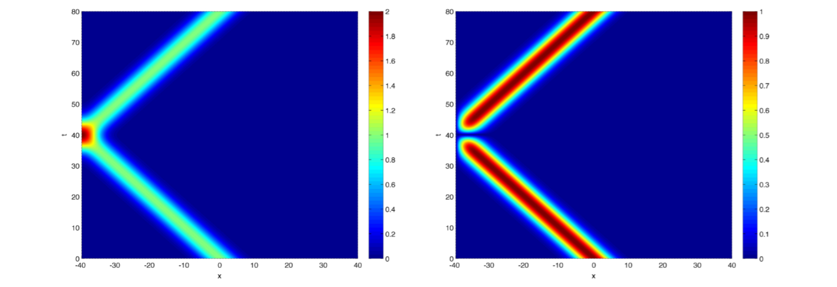
Figure 2: Reflection of a left-propagating wave at a mirror located at the left extremity of the computational domain: homogeneous Neumann boundary conditions (left), homogeneous Dirichlet boundary conditions (right).

In cases where only one mirror is considered, we impose outgoing Sommerfeld boundary conditions at the other end of the computational domain. These conditions are only approximately absorbing, but we make sure that this other extremity is sufficiently far away so that before the final time $T$, the solution may reach it but the spurious reflected wave will not have time to come back to the points at which we measure the amplitude of the solution and the energy flux.

We aim at observing solutions whose amplitude increases exponentially in time. This requires choosing a well-adapted time step. As an illustration of this, let us consider the very simple first-order differential equation $y^{\prime}(t)=\alpha y(t)$ ($t\geq 0$), with initial data $y(0)=y_{0}$ and where $\alpha>0$. In this case, the exact solution $y(t)=e^{\alpha t}y_{0}$ grows exponentially. Looking for an approximate solution $y^{n}\approx y(t_{n})$ computed by means of the time discretisation given above, we obtain the following numerical scheme

$$\Big{(}1-\frac{\alpha\delta t}{2}\Big{)}y^{n+1}=\Big{(}1+\frac{\alpha\delta t}{2}\Big{)}y^{n}\,.$$

The value of the approximate solution at computational time $T=t_{N}=N\delta t$ is explicitly given by

$$y^{N}=\left(\frac{1+\frac{\alpha\delta t}{2}}{1-\frac{\alpha\delta t}{2}}\right)^{N}y_{0}$$

which turns out to be an approximation of $e^{\alpha T}y_{0}$. By Taylor expansion with respect to $\delta t$, one finds that

$$\frac{y^{N}-y(T)}{y(T)} = \exp\Bigg{(}N\left(\log\left(1+\frac{\alpha\delta t}{2}\right)-\log\left(1-\frac{\alpha\delta t}{2}\right)\right)-\alpha T\Bigg{)}-1$$

$$= \exp\Big{(}\frac{1}{12}\alpha^{3}T\delta t^{2}+{\cal O}(\delta t^{3})\Big{)}-1$$

$$\simeq \frac{1}{12}\alpha^{3}T\delta t^{2}\mbox{ for }T\mbox{ fixed and }\delta t\rightarrow 0\,.$$

The numerical growth rate differs from the exact one, and the relative error at time $T$ is of magnitude $\frac{1}{12}\alpha^{3}T\delta t^{2}$. When dealing with a given final time $T\gg 1$ in order to study long time asymptotics, one has to prescribe a time step in such a way that $\frac{1}{12}\alpha^{3}T\delta t^{2}\ll 1$. One can notice that the accuracy of the profile is governed by the value of $\alpha\delta t=:x$, which is involved in the two factors $e^{\alpha\delta t}$ and $(1+\frac{\alpha\delta t}{2})/(1-\frac{\alpha\delta t}{2})$. A plot of the two corresponding functions is given with respect to $x$ in Figure 4, clearly showing the different behaviour as $x$ becomes large.

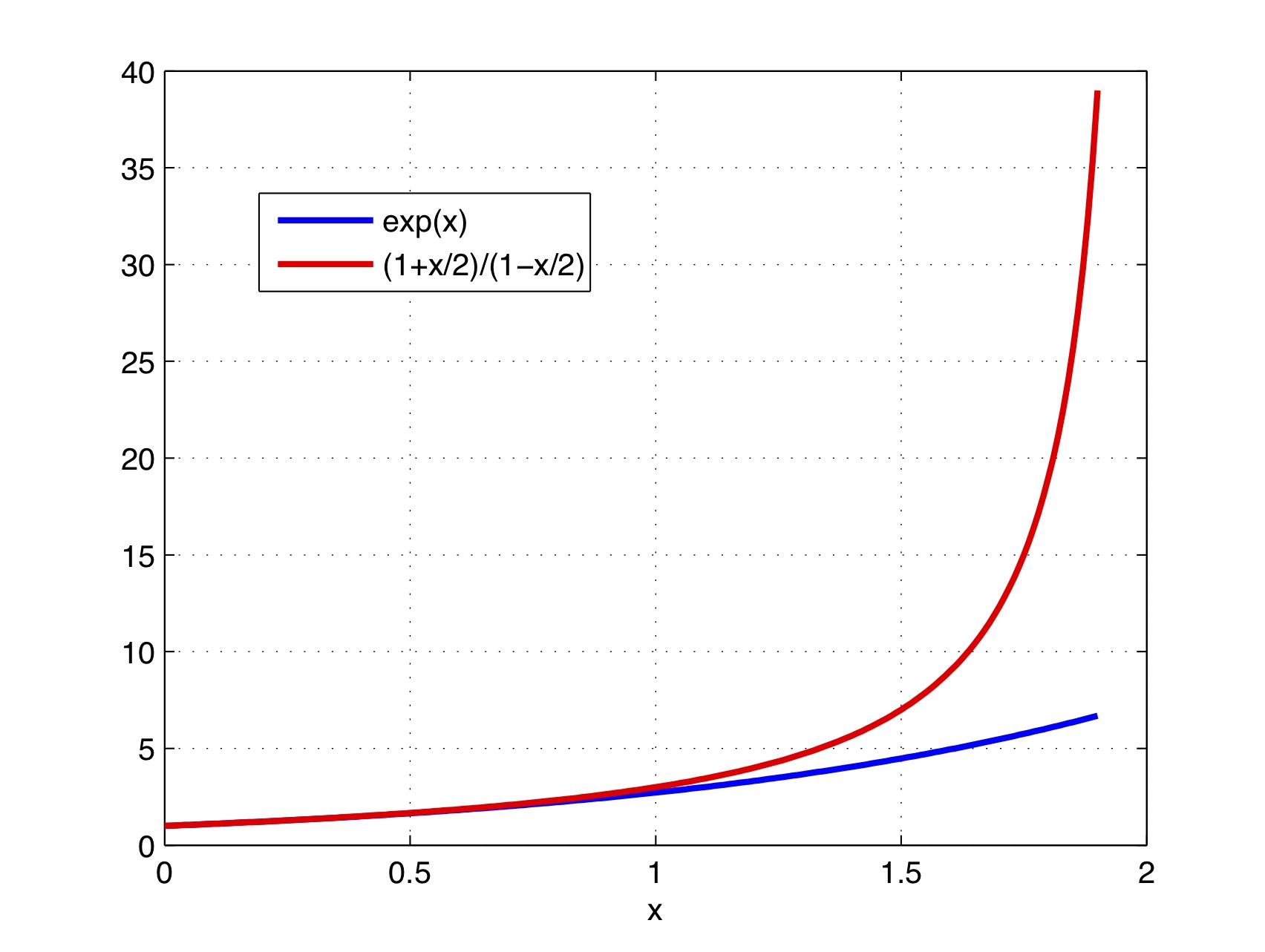
Figure 3: Plots of the two functions $e^{x}$ and $\frac{1+x/2}{1-x/2}$ for $x\in[0,2[$.

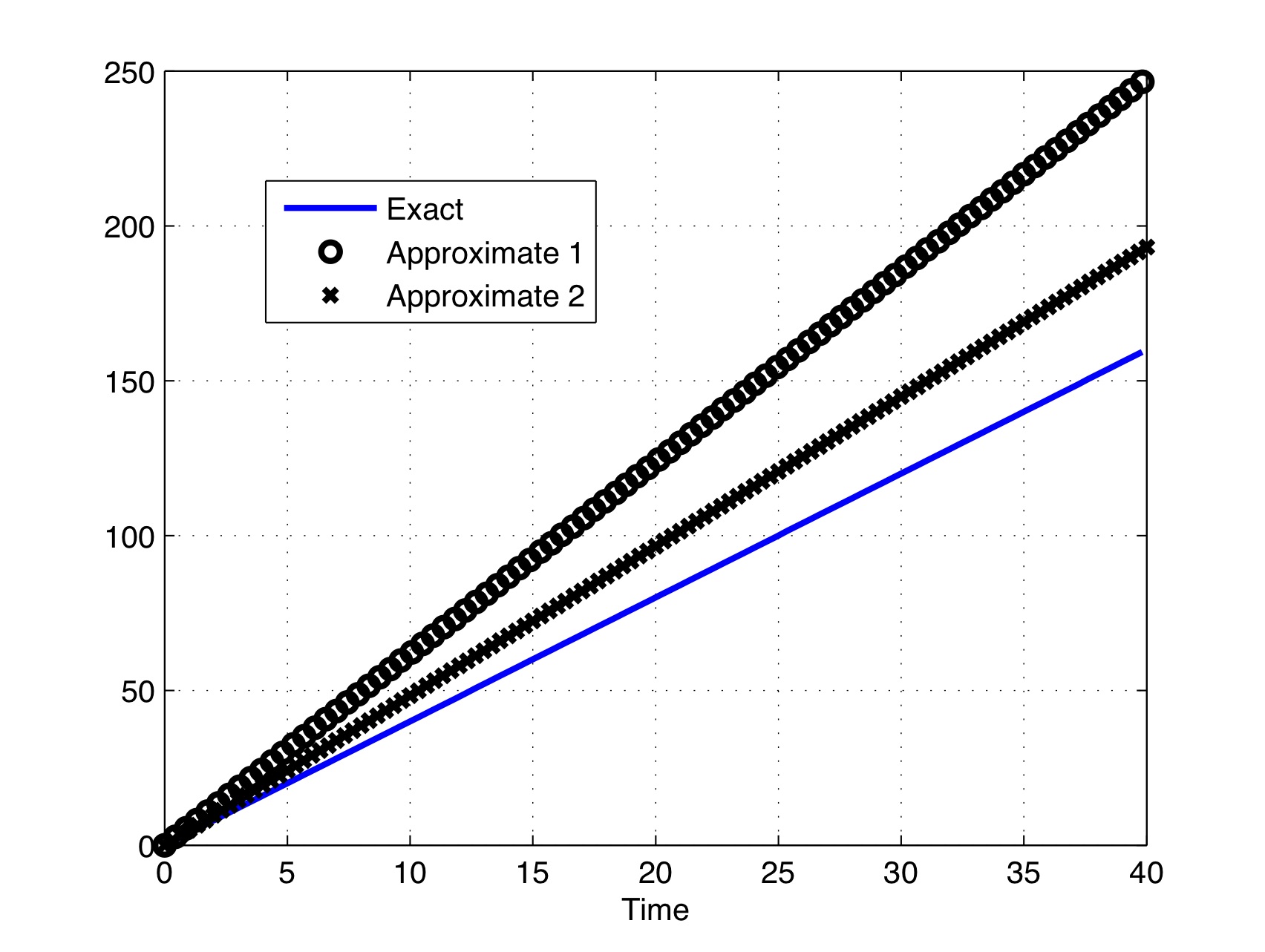
Figure 4: log of the solution: exact profile and profiles computed with $x=7/4$, $x=3/2$.

Furthermore, we plot in Figure 4 the logarithm of the time evolution of the solution, comparing the exact profile with two numerical values considered with the two cases $x=7/4$ and $x=3/2$. In each case, there is an amplification of the exponential growth that appears to be larger for large $x$. As these experiments clearly show, the value of $\delta t$ has to be moderate enough in order to measure accurately the exponential growth of the solution.

We shall observe the linear instability caused by the presence of the mirror, not only by measuring the amplitude of the wave, but also by computing the outgoing energy gain through a fixed sphere. In order to do so in a meaningful manner, we have to be careful with the way we evaluate the energy in the discrete case. In what follow, we present a discrete version of the energy that is numerically conserved and grants the validity of our numerical strategy.

4.3 Discrete energy conservation on the whole space

We first deal with (26) that is written for all indices $j\in\mathbb{Z}$, meaning that we consider the discrete values $(u^{n},v^{n})=(u_{j}^{n},v_{j}^{n})_{j\in\mathbb{Z}}$. Thus, we study the energy conservation of the theoretical scheme, that differs from the one involving boundary conditions that will be implemented for numerical simulations.

Theorem 3.

For approximate solutions of (20) given by (23)-(24), the quantity

$$E_{n}=\frac{1}{2}\sum_{j\in{\mathbb{Z}}}\Big{(}|v_{j}^{n}|^{2}+\Big{|}\frac{u_{j+1}^{n}-u_{j}^{n}}{h}\Big{|}^{2}+P_{j}|u_{j}^{n}|^{2}\Big{)}+\sum_{j\in{\mathbb{Z}}}\Im(V_{j}\bar{u}_{j}^{n}v_{j}^{n})$$

is conserved for each index $n$.

Before proving this result, let us first notice that this discrete version of energy is nothing but a discretisation of the continuous energy given by (21) using an upwind discretisation of the space derivative of $u$. This shows that this energy is consistent with the exact one.

Proof.– We follow the exact same way of deriving the energy in terms of $u$ ad $v$ in the continuous case, as shown in the proof of Theorem 1. We first multiply (24) by $\bar{v}_{j}^{n+1/2}$, which gives

$$\frac{1}{2\delta t}\Big{(}v_{j}^{n+1}-v_{j}^{n}\Big{)}\Big{(}\bar{v}_{j}^{n+1}+\bar{v}_{j}^{n}\Big{)}-iV_{j}|v_{j}^{n+1/2}|^{2}\hskip 72.26999pt$$

$$\hskip 72.26999pt=\left(\frac{1}{h^{2}}\Big{(}u_{j+1}^{n+1/2}-2u_{j}^{n+1/2}+u_{j-1}^{n+1/2}\Big{)}\!\!-P_{j}u_{j}^{n+1/2}\right)\!\bar{v}_{j}^{n+1/2}.$$

Taking the real part gives us

$$\frac{1}{2\delta t}\Re\Big{(}\big{(}v_{j}^{n+1}-v_{j}^{n}\big{)}\Big{(}\bar{v}_{j}^{n+1}+\bar{v}_{j}^{n}\Big{)}\Big{)}=\alpha_{j}^{n}-\beta_{j}^{n},$$ (28)

with

$$\begin{array}[]{lll}\alpha_{j}^{n}&=&\displaystyle\frac{1}{h^{2}}\Re\Big{(}\big{(}u_{j+1}^{n+1/2}-2u_{j}^{n+1/2}+u_{j-1}^{n+1/2}\big{)}\bar{v}_{j}^{n+1/2}\Big{)}\\ &=&\displaystyle\frac{1}{h^{2}}\Re\Big{(}\big{(}u_{j+1}^{n+1/2}-2u_{j}^{n+1/2}+u_{j-1}^{n+1/2}\big{)}\big{(}\frac{1}{\delta t}\big{(}\bar{u}_{j}^{n+1}-\bar{u}_{j}^{n}\big{)}+iV_{j}\bar{u}_{j}^{n+1/2}\big{)}\Big{)},\end{array}$$

with $\bar{v}_{j}^{n+1/2}$ being expressed in terms of $\bar{u}_{j}^{n+1}$, $\bar{u}_{j}^{n}$, $\bar{u}_{j}^{n+1/2}$ and similarly

$$\beta_{j}^{n}=\Re\Big{(}P_{j}\Big{(}\frac{1}{\delta t}\big{(}\bar{u}_{j}^{n+1}-\bar{u}_{j}^{n}\big{)}u_{j}^{n+1/2}+iV_{j}|u_{j}^{n+1/2}|^{2}\Big{)}\Big{)}=\Re\Big{(}P_{j}\Big{(}\frac{1}{\delta t}\big{(}\bar{u}_{j}^{n+1}-\bar{u}_{j}^{n}\big{)}u_{j}^{n+1/2}\Big{)}\Big{)}.$$

We now give two technical lemmas that will be useful to simplify the computations. The first one can be seen as the discrete version of the relation $\Re(\partial_{t}v\bar{v})=\frac{1}{2}\partial_{t}|v|^{2}$:

Lemma 4.1.

One has

$$\frac{1}{2}\Re\Big{(}(v_{j}^{n+1}-v_{j}^{n})(\bar{v}_{j}^{n+1}+\bar{v}_{j}^{n})\Big{)}=\frac{1}{2}\Big{(}|v_{j}^{n+1}|^{2}-|v_{j}^{n}|^{2}\Big{)}.$$ (29)

Proof.– Developing the proposed expression simply leads us to

$$\Re\Big{(}(v_{j}^{n+1}-v_{j}^{n})(\bar{v}_{j}^{n+1}+\bar{v}_{j}^{n})\Big{)}=\Re(v_{j}^{n+1}\bar{v}_{j}^{n+1}-v_{j}^{n}\bar{v}_{j}^{n+1}+v_{j}^{n+1}\bar{v}_{j}^{n}-v_{j}^{n}\bar{v}_{j}^{n})=|v_{j}^{n+1}|^{2}-|v_{j}^{n}|^{2}$$

since $v_{j}^{n}\bar{v}_{j}^{n+1}$ and $v_{j}^{n+1}\bar{v}_{j}^{n}$ are complex-conjugated. The lemma is proved. ∎

The second lemma can be interpreted as the discrete version of an integration by parts:

Lemma 4.2.

One has

$$\Re\Big{(}\sum_{j\in{\mathbb{Z}}}(u_{j+1}^{n+1/2}-2u_{j}^{n+1/2}+u_{j-1}^{n+1/2})(\bar{u}_{j}^{n+1}-\bar{u}_{j}^{n})\Big{)}=-\frac{1}{2}\sum_{j\in{\mathbb{Z}}}\left(\big{|}u_{j+1}^{n+1}-u_{j}^{n+1}\big{|}^{2}-\big{|}u_{j+1}^{n}-u_{j}^{n}\big{|}^{2}\right).$$ (30)

Proof.– We have for each index $j$

$$\begin{array}[]{lll}&\Re\Big{(}(u_{j+1}^{n+1/2}-2u_{j}^{n+1/2}+u_{j-1}^{n+1/2})(\bar{u}_{j}^{n+1}-\bar{u}_{j}^{n})\Big{)}\\ =&\frac{1}{2}\Re\Big{(}u_{j+1}^{n+1}\bar{u}_{j}^{n+1}-2|u_{j}^{n+1}|^{2}+u_{j-1}^{n+1}\bar{u}_{j}^{n+1}-u_{j+1}^{n+1}\bar{u}_{j}^{n}+2u_{j}^{n+1}\bar{u}_{j}^{n}-u_{j-1}^{n+1}\bar{u}_{j}^{n}\\ &~{}~{}+u_{j+1}^{n}\bar{u}_{j}^{n+1}-2u_{j}^{n}\bar{u}_{j}^{n+1}+u_{j-1}^{n}\bar{u}_{j}^{n+1}-u_{j+1}^{n}\bar{u}_{j}^{n}+2|u_{j}^{n}|^{2}-u_{j-1}^{n}\bar{u}_{j}^{n}\Big{)}\\ =&\frac{1}{2}\Re\Big{(}u_{j+1}^{n+1}\bar{u}_{j}^{n+1}-2|u_{j}^{n+1}|^{2}+u_{j-1}^{n+1}\bar{u}_{j}^{n+1}-u_{j+1}^{n+1}\bar{u}_{j}^{n}-u_{j-1}^{n+1}\bar{u}_{j}^{n}\\ &~{}~{}+u_{j+1}^{n}\bar{u}_{j}^{n+1}+u_{j-1}^{n}\bar{u}_{j}^{n+1}-u_{j+1}^{n}\bar{u}_{j}^{n}+2|u_{j}^{n}|^{2}-u_{j-1}^{n}\bar{u}_{j}^{n}\Big{)}.\end{array}$$

Taking the sum over ${\mathbb{Z}}$ leads to

$$\begin{array}[]{lll}&\displaystyle\Re\Big{(}\sum_{j\in{\mathbb{Z}}}(u_{j+1}^{n+1/2}-2u_{j}^{n+1/2}+u_{j-1}^{n+1/2})(\bar{u}_{j}^{n+1}-\bar{u}_{j}^{n})\Big{)}\\ =&\displaystyle\frac{1}{2}\Re\Big{(}\sum_{j\in{\mathbb{Z}}}\Big{(}u_{j+1}^{n+1}\bar{u}_{j}^{n+1}-2|u_{j}^{n+1}|^{2}+u_{j}^{n+1}\bar{u}_{j+1}^{n+1}-u_{j+1}^{n+1}\bar{u}_{j}^{n}-u_{j}^{n+1}\bar{u}_{j+1}^{n+1}\\ &~{}~{}~{}~{}~{}~{}~{}~{}~{}~{}~{}+u_{j+1}^{n}\bar{u}_{j}^{n+1}+u_{j}^{n}\bar{u}_{j+1}^{n+1}-u_{j+1}^{n}\bar{u}_{j}^{n}+2|u_{j}^{n}|^{2}-u_{j}^{n}\bar{u}_{j+1}^{n}\Big{)}\Big{)},\end{array}$$

using an index translation as often as required to get rid of $j-1$ contributions. If we simplify this expression taking into account all the complex conjugations, it leads to

$$\begin{array}[]{lll}&\displaystyle\Re\Big{(}\sum_{j\in{\mathbb{Z}}}(u_{j+1}^{n+1/2}-2u_{j}^{n+1/2}+u_{j-1}^{n+1/2})(\bar{u}_{j}^{n+1}-\bar{u}_{j}^{n})\Big{)}\\ =&-\displaystyle\frac{1}{2}\Re\Big{(}\sum_{j\in{\mathbb{Z}}}\Big{(}\big{(}2|u_{j}^{n+1}|^{2}-2u_{j}^{n+1}\bar{u}_{j+1}^{n+1}\big{)}-\big{(}2|u_{j}^{n}|^{2}-2u_{j}^{n}\bar{u}_{j+1}^{n}\big{)}\Big{)}\Big{)}\\ =&\displaystyle-\frac{1}{2}\sum_{j\in{\mathbb{Z}}}\Big{(}\big{(}|u_{j+1}^{n+1}|^{2}+|u_{j}^{n+1}|^{2}-2\Re(u_{j}^{n+1}\bar{u}_{j+1}^{n+1})\big{)}-\big{(}|u_{j+1}^{n}|^{2}+|u_{j}^{n}|^{2}-2\Re(u_{j}^{n}\bar{u}_{j+1}^{n})\big{)}\Big{)}\\ =&\displaystyle-\frac{1}{2}\sum_{j\in{\mathbb{Z}}}\Big{(}|u_{j+1}^{n+1}-u_{j}^{n+1}|^{2}-|u_{j+1}^{n}-u_{j}^{n}|^{2}\Big{)},\end{array}$$

which proves the lemma. ∎

Using Lemma 30 gives

$$\begin{array}[]{lll}\displaystyle\sum_{j\in{\mathbb{Z}}}\alpha_{j}^{n}\!\!\!\!\!&=&\!\!\!\!\!\!\displaystyle-\sum_{j\in{\mathbb{Z}}}\left(\frac{1}{2}\frac{1}{\delta t}\frac{\left|u_{j+1}^{n+1}-u_{j}^{n+1}\right|^{2}-\left|u_{j+1}^{n}-u_{j}^{n}\right|^{2}}{h^{2}}-\Re\left(\frac{i}{h^{2}}\Big{(}u_{j+1}^{n+1/2}-2u_{j}^{n+1/2}+u_{j-1}^{n+1/2}\Big{)}V_{j}\bar{u}_{j}^{n+1/2}\right)\right)\\ ~{}\!\!\!\!\!&=&\!\!\!\!\!\!-\displaystyle\sum_{j\in{\mathbb{Z}}}\left(\frac{1}{2}\frac{1}{\delta t}\frac{\left|u_{j+1}^{n+1}-u_{j}^{n+1}\right|^{2}-\left|u_{j+1}^{n}-u_{j}^{n}\right|^{2}}{h^{2}}+\Im\left(\frac{1}{h^{2}}\Big{(}u_{j+1}^{n+1/2}-2u_{j}^{n+1/2}+u_{j-1}^{n+1/2}\Big{)}V_{j}\bar{u}_{j}^{n+1/2}\right)\right).\end{array}$$

We then express the second-order finite difference term with respect to $v$. It gives

$$\begin{array}[]{lll}{}&&\displaystyle\Im\left(\frac{1}{h^{2}}\Big{(}u_{j+1}^{n+1/2}-2u_{j}^{n+1/2}+u_{j-1}^{n+1/2}\Big{)}\par V_{j}\bar{u}_{j}^{n+1/2}\right)\\ &=&\displaystyle\Im\left(\Big{(}\frac{1}{\delta t}\Big{(}v_{j}^{n+1}-v_{j}^{n}\Big{)}-iV_{j}v_{j}^{n+1/2}+P_{j}u_{j}^{n+1/2}\Big{)}V_{j}\bar{u}_{j}^{n+1/2}\right)\\ &=&\displaystyle\Im\left(\frac{1}{\delta t}\Big{(}v_{j}^{n+1}-v_{j}^{n}\Big{)}V_{j}\bar{u}_{j}^{n+1/2}-iV_{j}v_{j}^{n+1/2}V_{j}\bar{u}_{j}^{n+1/2}\right).\\ \end{array}$$

Since $-iV_{j}\bar{u}_{j}^{n+1/2}=\frac{1}{\delta t}(\bar{u}_{j}^{n+1}-\bar{u}_{j}^{n})-\bar{v}_{j}^{n+1/2}$, this implies

$$\begin{array}[]{lll}{}&&\displaystyle\Im\left(\frac{1}{h^{2}}\Big{(}u_{j+1}^{n+1/2}-2u_{j}^{n+1/2}+u_{j-1}^{n+1/2}\Big{)}V_{j}\bar{u}_{j}^{n+1/2}\right)\\ &=&\displaystyle\Im\left(\frac{1}{\delta t}\Big{(}v_{j}^{n+1}-v_{j}^{n}\Big{)}V_{j}\bar{u}_{j}^{n+1/2}+\frac{1}{\delta t}\Big{(}\bar{u}_{j}^{n+1}-\bar{u}_{j}^{n}\Big{)}V_{j}v_{j}^{n+1/2}+V_{j}\big{|}v_{j}^{n+1/2}\big{|}^{2}\right)\\ &=&\displaystyle\Im\left(V_{j}\Big{(}\frac{1}{\delta t}\Big{(}v_{j}^{n+1}-v_{j}^{n}\Big{)}\bar{u}_{j}^{n+1/2}+\frac{1}{\delta t}\Big{(}\bar{u}_{j}^{n+1}-\bar{u}_{j}^{n}\Big{)}v_{j}^{n+1/2}\Big{)}\right).\displaystyle\end{array}$$

Rewriting now

$$\begin{array}[]{lll}&&\Im\Big{(}V_{j}\Big{(}v_{j}^{n+1}-v_{j}^{n}\Big{)}\bar{u}_{j}^{n+1/2}+\Big{(}\bar{u}_{j}^{n+1}-\bar{u}_{j}^{n}\Big{)}v_{j}^{n+1/2}\Big{)}\\ \vspace*{-0.2cm}\\ &=&\displaystyle\frac{1}{2}\Im\Big{(}V_{j}(v_{j}^{n+1}\bar{u}_{j}^{n+1}+v_{j}^{n+1}\bar{u}_{j}^{n}-v_{j}^{n}\bar{u}_{j}^{n+1}-v_{j}^{n}\bar{u}_{j}^{n}+\bar{u}_{j}^{n+1}v_{j}^{n+1}+\bar{u}_{j}^{n+1}v_{j}^{n}-\bar{u}_{j}^{n}v_{j}^{n+1}-\bar{u}_{j}^{n}v_{j}^{n})\Big{)}\\ \vspace*{-0.2cm}\\ &=&\displaystyle\frac{1}{2}\Im\Big{(}V_{j}(v_{j}^{n+1}\bar{u}_{j}^{n+1}-v_{j}^{n}\bar{u}_{j}^{n}+\bar{u}_{j}^{n+1}v_{j}^{n+1}-\bar{u}_{j}^{n}v_{j}^{n})\Big{)}=\Im\Big{(}V_{j}(\bar{u}_{j}^{n+1}v_{j}^{n+1}-\bar{u}_{j}^{n}v_{j}^{n})\Big{)},\end{array}$$

it follows that

$$\sum_{j\in{\mathbb{Z}}}\alpha_{j}^{n}=-\frac{1}{\delta t}\sum_{j\in{\mathbb{Z}}}\Bigg{(}\frac{1}{2}\frac{\left|u_{j+1}^{n+1}-u_{j}^{n+1}\right|^{2}-\left|u_{j+1}^{n}-u_{j}^{n}\right|^{2}}{h^{2}}+\Im\Big{(}V_{j}(\bar{u}_{j}^{n+1}v_{j}^{n+1}-\bar{u}_{j}^{n}v_{j}^{n})\Big{)}\Bigg{)}.$$

Using Lemma 29, we also express the sum of all $\beta_{j}^{n}$ as

$$\sum_{j\in{\mathbb{Z}}}\beta_{j}^{n}=\frac{1}{2}\frac{1}{\delta t}\sum_{j\in{\mathbb{Z}}}P_{j}\Big{(}|u_{j}^{n+1}|^{2}-|u_{j}^{n}|^{2}\Big{)}.$$

Finally, summing (28) over all indices $j$ and separating $n+1$ contributions in the left-hand side and $n$ contributions in the right-hand side, we find that

$$\begin{array}[]{lll}{}&&\displaystyle\frac{1}{\delta t}\sum_{j\in{\mathbb{Z}}}\Big{(}\frac{1}{2}\Big{(}|v_{j}^{n+1}|^{2}+\Big{|}\frac{u_{j+1}^{n+1}-u_{j}^{n+1}}{h}\Big{|}^{2}+P_{j}|u_{j}^{n+1}|^{2}\Big{)}+\Im(V_{j}\bar{u}_{j}^{n+1}v_{j}^{n+1})\Big{)}\\ &=&\displaystyle\frac{1}{\delta t}\sum_{j\in{\mathbb{Z}}}\Big{(}\frac{1}{2}\Big{(}|v_{j}^{n}|^{2}+\Big{|}\frac{u_{j+1}^{n}-u_{j}^{n}}{h}\Big{|}^{2}+P_{j}|u_{j}^{n}|^{2}\Big{)}+\Im(V_{j}\bar{u}_{j}^{n}v_{j}^{n})\Big{)},\end{array}$$

which completes the proof of Theorem 3. ∎

Note that the successive steps in this proof are similar to the ones that have been used for the conservation of energy in the continuous case.

Let us point out that this discrete conservation holds for the exact solution of the semi-implicit numerical scheme. However, one needs to use a linear algebra routine in order to calculate the solution $(u^{n+1},v^{n+1})$, solving a linear system. This means that the obtained numerical solution solves (23)-(24) up to some numerical error. It follows that the discrete energy calculated with the computed $(u^{n+1},v^{n+1})$ is not exactly conserved. It can be also noticed that the discrete version of the space derivative is a good approximation of the exact one only if the space step is small enough. It turns out that there may be a discrepancy between the exact energy and the approximate one (exactly conserved by the exact solution $(u^{n},v^{n})$ given by (23) and (24)) when dealing with highly oscillating functions.

4.4 Influence of boundary conditions on energy conservation

In numerical experiments, the finite difference scheme (23)-(24) is always used on a bounded domain for obvious reasons. We now analyse how this affects the energy conservation. For the sake of simplicity, we first deal here with the half-line $[0,+\infty[$, that requires to calculate the values $u_{j}^{n}$ and $v_{j}^{n}$ for nonnegative values of indices $j$. Taking bounded domain $\Omega$ will lead us to similar considerations on the opposite extremity.

We first assume that the Dirichlet boundary condition $u(t,0)=0$ is prescribed at each time. The following proposition shows that the discrete version of the classical integration by parts

$$\int_{0}^{+\infty}\partial_{x}^{2}u\,\bar{u}\,{\mathrm{d}}x=-\int_{0}^{+\infty}|\partial_{x}u|^{2}\,{\mathrm{d}}x$$

(when $u(t,0)=0$ and $u(t,x)=0$ if $x\gg 1$) still holds. From now on, the quantity $u$ is assumed to depend only on the space index $j$.

Proposition 4.1.

Let $w_{j}$ denote the approximation of the second derivative of $u$ at index $j$ computed in terms of $(u_{k})_{k\geq 1}$. We then have

$$\sum_{j=1}^{+\infty}w_{j}\bar{u}_{j}=-\frac{1}{h^{2}}|u_{1}|^{2}-\sum_{j=2}^{+\infty}\Big{|}\frac{u_{j}-u_{j-1}}{h}\Big{|}^{2}.$$

Proof.– Setting $w_{1}=(u_{2}-2u_{1})/h^{2}$ (by consistency with (25)) and $w_{j}=(u_{j+1}-2u_{j}+u_{j-1})/h^{2}$ for $j\geq 2$ (using (22)), we have

$$\begin{array}[]{lll}\displaystyle\sum_{j=1}^{+\infty}w_{j}\bar{u}_{j}&=&\displaystyle\frac{1}{h^{2}}\Big{(}(u_{2}-2u_{1})\bar{u}_{1}+\sum_{j=2}^{+\infty}(u_{j+1}-2u_{j}+u_{j-1})\bar{u}_{j}\Big{)}\\ &=&\displaystyle\frac{1}{h^{2}}\Big{(}u_{2}\bar{u}_{1}-2|u_{1}|^{2}-2\sum_{j=2}^{+\infty}|u_{j}|^{2}+\sum_{j=2}^{+\infty}u_{j+1}\bar{u}_{j}+\sum_{j=2}^{+\infty}u_{j-1}\bar{u}_{j}\Big{)}\\ &=&\displaystyle\frac{1}{h^{2}}\Big{(}-|u_{1}|^{2}-\sum_{j=2}^{+\infty}|u_{j}|^{2}-\sum_{j=2}^{+\infty}|u_{j-1}|^{2}+2\Re\Big{(}\sum_{j=2}^{+\infty}u_{j-1}\bar{u}_{j}\Big{)}\Big{)}\\ &=&\displaystyle\frac{1}{h^{2}}\Big{(}-|u_{1}|^{2}-\sum_{j=2}^{+\infty}|u_{j}-u_{j-1}|^{2}\Big{)}.\end{array}$$

Hence, the proposition is proved. ∎

Note that when dealing with Dirichlet boundary conditions, it can be assumed that the value at $x=0$ is always $u_{0}=0$. Consequently, the identity of Proposition 4.1 can be rewritten as

$$\sum_{j=0}^{+\infty}w_{j}\bar{u}_{j}=-\sum_{j=1}^{+\infty}\Big{|}\frac{u_{j}-u_{j-1}}{h}\Big{|}^{2}.$$

It turns out that all the computations performed in the proof of Theorem 3 remain valid and the discrete conservation of the invariant computed on the positive half-line still holds. The same considerations made on the right extremity of the domain lead us to the conservation of the energy computed on $\Omega$, as states the

Theorem 4.

For approximate solutions of (20) given by (23)-(24) computed on spatial points $x_{j}=a+jh$ ($j\in\left\{0,\ldots,J+1\right\}$) with Dirichlet conditions for $u$ at the boundary (that is $u_{0}^{n}=u_{J+1}^{n}=0$ for each $n\geq 0$), the quantity

$$E_{n}=\frac{1}{2}\sum_{j=1}^{J}\Big{(}|v_{j}^{n}|^{2}+\Big{|}\frac{u_{j+1}^{n}-u_{j}^{n}}{h}\Big{|}^{2}+P_{j}|u_{j}^{n}|^{2}\Big{)}+\sum_{j=1}^{J}\Im(V_{j}\bar{u}_{j}^{n}v_{j}^{n})$$

is conserved for each index $n$.

It can be noticed that only boundary conditions on $u$ are used in the integration by parts. But since $\partial_{t}u-iVu=v$, if Dirichlet conditions are prescribed for $u$, it can be seen that $v$ also satisfies Dirichlet conditions at the boundary.

We then consider the Neumann boundary condition $\partial_{x}u(t,0)=0$. We show here a slight modification in the conservation of energy that differs from what has been obtained in the case of Dirichlet conditions.

Proposition 4.2.

Let $w_{j}$ denote the approximation of the second derivative of $u$ at index $j$ computed in terms of $(u_{k})_{k\geq 0}$. We then have

$$\frac{1}{2}w_{0}\bar{u}_{0}+\sum_{j=1}^{+\infty}w_{j}\bar{u}_{j}=-\sum_{j=1}^{+\infty}\Big{|}\frac{u_{j}-u_{j-1}}{h}\Big{|}^{2}.$$

Proof.– We now have $w_{0}=2(u_{1}-u_{0})/h^{2}$ (by consistency with (27)) and $w_{j}=(u_{j+1}-2u_{j}+u_{j-1})/h^{2}$ for $j\geq 1$ (using (22)). From this, the discrete sum now expresses as

$$\begin{array}[]{lll}\displaystyle\frac{1}{2}\frac{2(u_{1}-u_{0})}{h^{2}}\bar{u}_{0}+\sum_{j=1}^{+\infty}w_{j}\bar{u}_{j}&=&\displaystyle\frac{1}{h^{2}}\Big{(}u_{1}\bar{u}_{0}-|u_{0}|^{2}+\sum_{j=1}^{+\infty}(u_{j+1}-2u_{j}+u_{j-1})\bar{u}_{j}\Big{)}\\ &=&\displaystyle\frac{1}{h^{2}}\Big{(}u_{1}\bar{u}_{0}-|u_{0}|^{2}-2\sum_{j=1}^{+\infty}|u_{j}|^{2}+\sum_{j=1}^{+\infty}u_{j+1}\bar{u}_{j}+\sum_{j=1}^{+\infty}u_{j-1}\bar{u}_{j}\Big{)}\\ &=&\displaystyle\frac{1}{h^{2}}\Big{(}-\sum_{j=1}^{+\infty}|u_{j}|^{2}-\sum_{j=1}^{+\infty}|u_{j-1}|^{2}+2\Re\Big{(}\sum_{j=1}^{+\infty}u_{j-1}\bar{u}_{j}\Big{)}\Big{)}\\ &=&\displaystyle-\frac{1}{h^{2}}\sum_{j=1}^{+\infty}|u_{j}-u_{j-1}|^{2}.\end{array}$$

Hence, the proposition is proved. ∎

Note that in this case, for a bounded domain with spatial points $x_{0}=0$, $\ldots$, $x_{j}=a+jh$, $\ldots$, $x_{J+1}=L$, we deal with the approximation

$$\int_{0}^{L}f(x)\,{\mathrm{d}}x\approx h\Big{(}\frac{1}{2}f(0)+\sum_{j=1}^{J}f(x_{j})+\frac{1}{2}f(L)\Big{)}$$ (31)

which involves the second-order trapezoidal rule. Taking into account Proposition 4.2 and using similar arguments at the right boundary $x=L$, we obtain the following

Theorem 5.

For approximate solutions of (20) given by (23)-(24) computed on spatial points $x_{j}=a+jh$ ($j\in\left\{0,\ldots,J+1\right\}$) with Neumann conditions at the boundary, the quantity

$$\begin{array}[]{lll}E_{n}&=&\displaystyle\frac{1}{4}\Big{(}|v_{0}^{n}|^{2}+|v_{J+1}^{n}|^{2}+P_{0}|u_{0}^{n}|^{2}+P_{J+1}|u_{J+1}^{n}|^{2}\Big{)}+\frac{1}{2}\Big{(}\Im(V_{0}\bar{u}_{0}^{n}v_{0}^{n})+\Im(V_{J+1}\bar{u}_{J+1}^{n}v_{J+1}^{n})\Big{)}\\ &+&\displaystyle\frac{1}{2}\sum_{j=1}^{J}\Big{(}|v_{j}^{n}|^{2}+\Big{|}\frac{u_{j+1}^{n}-u_{j}^{n}}{h}\Big{|}^{2}+P_{j}|u_{j}^{n}|^{2}\Big{)}+\sum_{j=1}^{J}\Im(V_{j}\bar{u}_{j}^{n}v_{j}^{n})\end{array}$$

is conserved for each index $n$.

Once again, the proof relies on the computations that have already been performed in the whole space, with a $\frac{1}{2}$ coefficient for quantities evaluated at indices $J=0$ and $j=J+1$. It can be noticed that the conservation of energy for Dirichlet conditions is a particular case of the use of formula (31) when boundary terms vanish, leading us to the sum between $1$ and $J$ in Theorem 4.

5 Numerical experiments

We now present and discuss numerical simulations in all cases (type I, II, and III) using the numerical scheme that has been previously described. The solutions are evolved numerically on the bounded domain that now writes $[R_{-},R_{+}]_{r_{*}}$. We choose $R_{a},R_{f}\in\mathopen{]}R_{-},R_{+}[$ and we measure two types of quantities:

1. the amplitude of the solution at $r_{*}=R_{a}$ at all times;

2. the outgoing energy flux across the $r_{*}=R_{f}$ hypersurface at all times; in fact we measure the energy gain at all times, which is given by the outgoing energy ${\cal F}_{[0,t]\times S_{R_{0}}}$ divided by the energy of the initial data, i.e.

   $${\cal G}_{R_{0}}(t)=\frac{{\cal F}_{[0,t]\times S_{R_{0}}}}{{\cal F}_{\tilde{\Sigma}_{0}}}\,.$$ (32)

For type I black hole bombs, $R_{+}=R_{1}$ and the mirror is at $r_{*}=R_{+}$; for type II bombs, $R_{-}=R_{1}$ and the mirror is located at $r_{*}=R_{-}$; in the case of type III bombs, we have one mirror at $R_{-}=R_{1}$ and another at $R_{+}=R_{2}$ (see (16), (17), and (18) for the description of the boundary initial value problems corresponding to each type of bomb).

5.1 Black hole bombs of type II

We investigate Type II bombs on a Reissned-Norstr m and a de Sitter-Reissner-Nordstr m background.

• For the Reissner-Nordstr m case, the values of the parameters are $M=2.001$ and $Q=2$ for the black hole and $q=1$, $m=0.1$, $l=0$ for the field. The solution has zero angular momentum and is therefore spherically symmetric. The black hole is close to being extreme, this is however not fundamental. We have observed a behaviour similar to the one displayed below for other choices of parameters. The presentation of this particular example was motivated by the fact that the results are more striking in this case. This is probably due to the fact that superradiance becomes stronger as one approaches the extreme case. For these values, the ergoregion spreads from $x=-\infty$ until a value between $30$ and $40$, as can be seen from the sign of the potential $P-V^{2}$ in Figure 5. For our “flare-like” Cauchy data, we have set

  $$\phi(0,.)\simeq 0\mbox{ and }\frac{\partial\phi}{\partial t}(0,x)=\phi_{1}(x)=e^{i\omega x/\alpha}e^{-((x-x_{0})/\alpha)^{2}}\,,$$ (33)

  with frequency $\omega=0$, scale factor $\alpha=5$, and translation coefficient $x_{0}=-20$, which ensures that the data are supported (for all practical purposes) within the ergoregion. We consider both Neumann and Dirichlet boundary conditions at the mirror. Computations are first performed until final time $T=100$ on the domain $[-40,120]$ discretised with $2,000$ spatial points. This allows to observe in details the beginning of the evolution (see Figure 6): the wave is reflected against the mirror and sends bursts out to infinity. It seems that the wave has a tendency to stay close to the mirror.

  

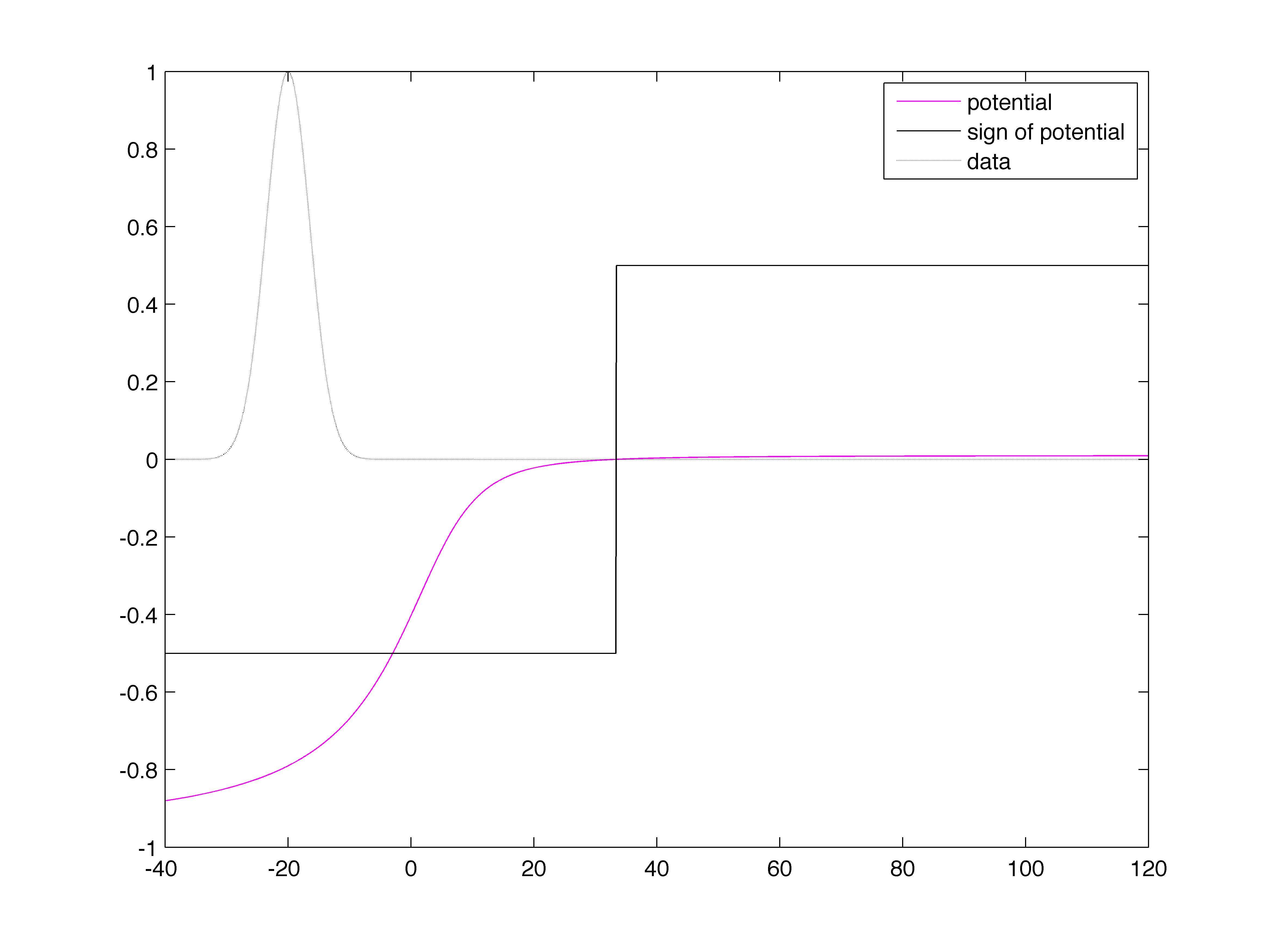
  Figure 5: Profile of data and potential.

  

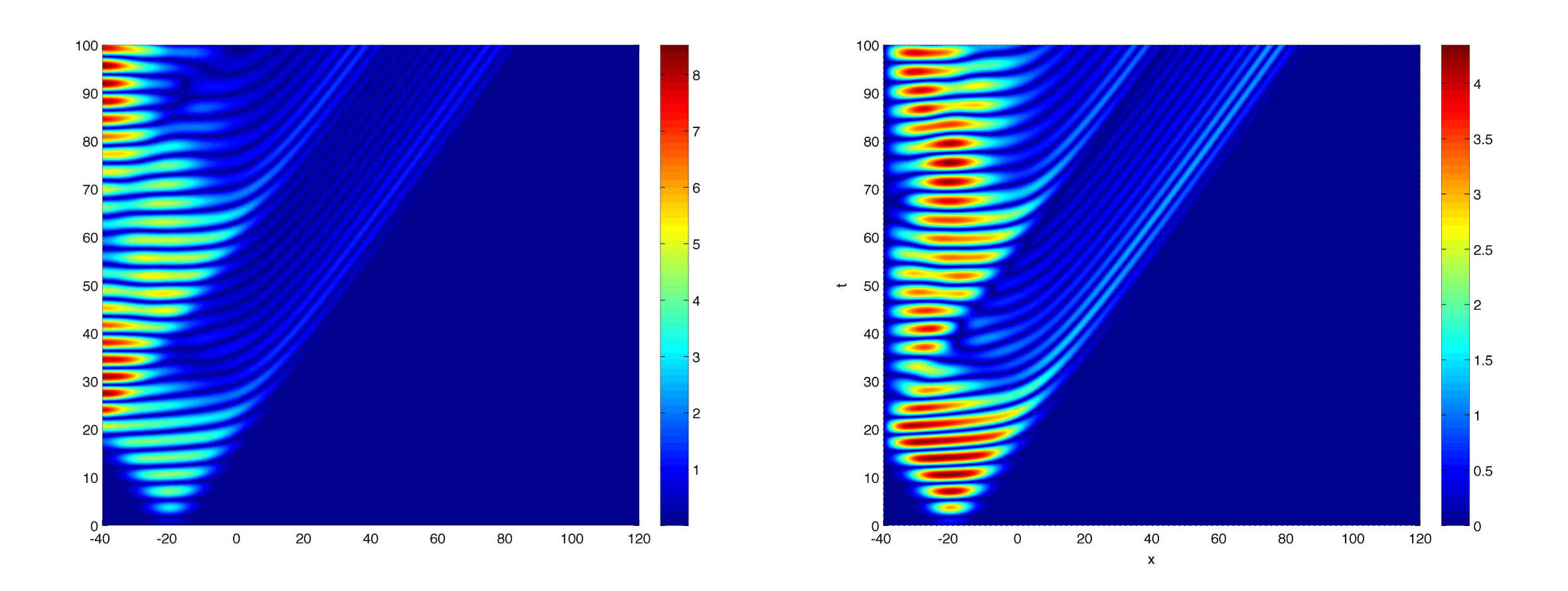
  Figure 6: $(x,t)$ isovalues of the solution: Neumann conditions (left), Dirichlet conditions (right).

  In order to observe the phenomenon for a longer time, we enlarge the computational domain to $[-40,920]$ with $4000$ points. A simulation up to $T=300$ with $\delta t=h$, displayed in Figure 7, confirms the early observations and indicates an amplification of the field with time. We then increase the number of spatial points to 40000 and perform the computation up to time $T=1500$. The amplitude of the field is measured at $x=-16$ and the outgoing energy flux at $x=56$. The evolution with time of the logarithm of the amplitude (precisely of the absolute value of the real part of the solution) and of the energy gain are displayed on Figures 8 and 9, establishing that both quantities increase exponentially in time.

  

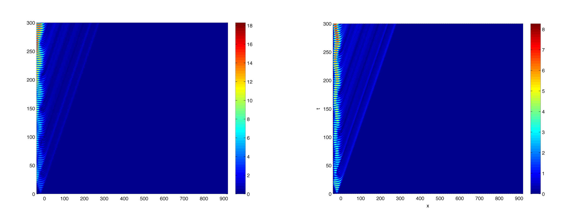
  Figure 7: $(x,t)$ isovalues of the solution: Neumann conditions (left), Dirichlet conditions (right).

  

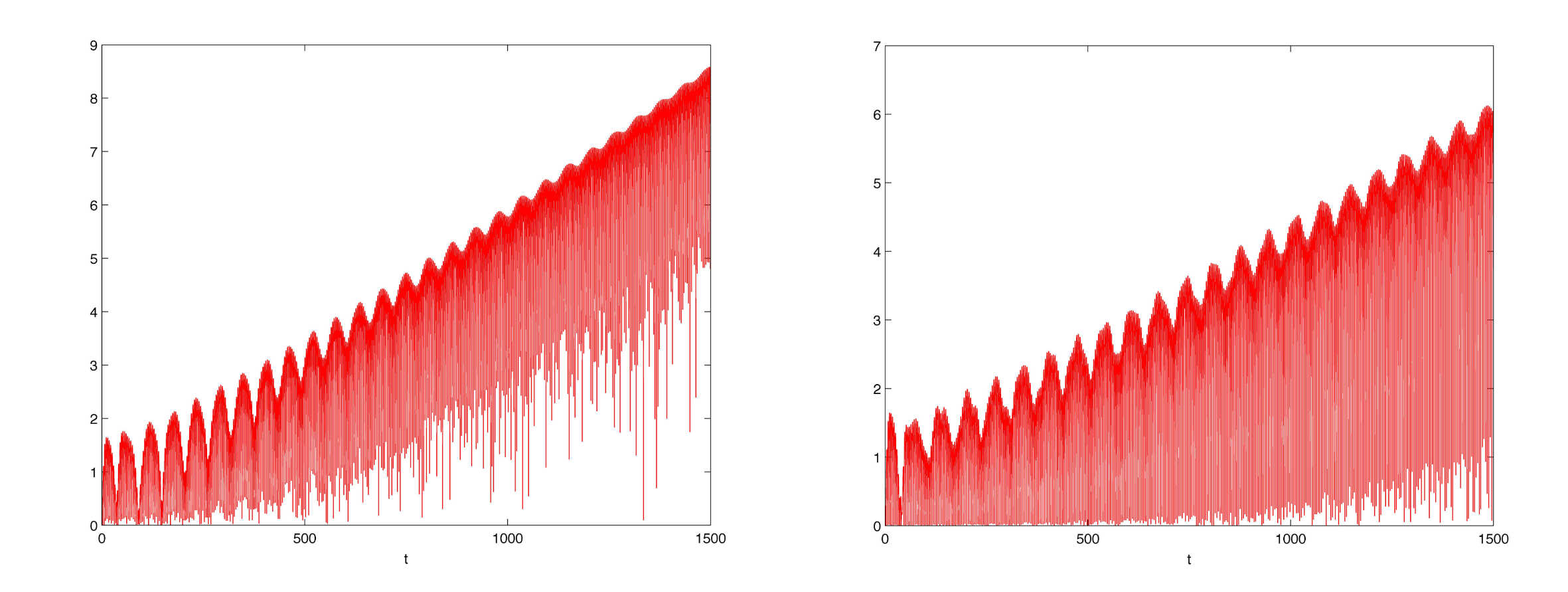
  Figure 8: Profile of the logarithm of the amplitude: Neumann conditions (left), Dirichlet conditions (right).

  

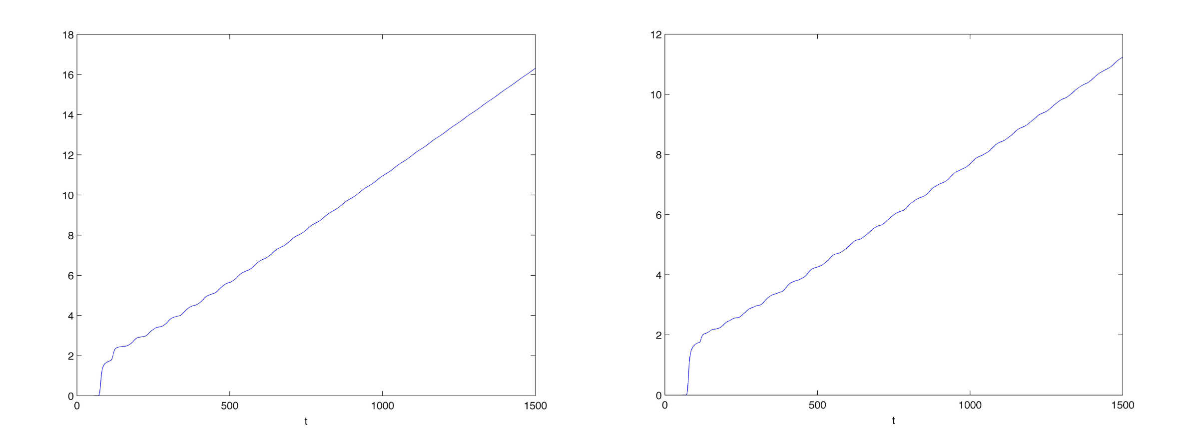
  Figure 9: Profile of logarithm of energy gain: Neumann conditions (left), Dirichlet conditions (right).

  The plots in Figure 9 exhibits two different regimes with two distinct exponential rates; the larger one briefly occurs at a transient stage and is followed by a smaller growth that seems to govern the asymptotics of the energy gain.

• We now investigate the case of a subextremal de Sitter Reissner-Nordstr m black hole, with parameters $Q=2$, $M=3$ and $\Lambda=1/(6M)^{2}$. The zeros of the function $F$ (calculated by dichotomy) are given by

  $$r_{n}=-20.5361916161634,~{}r_{-}=0.763697274361058,$$

  $$r_{0}=5.99999999996640,,~{}r_{+}=13.7724943418359.$$

  

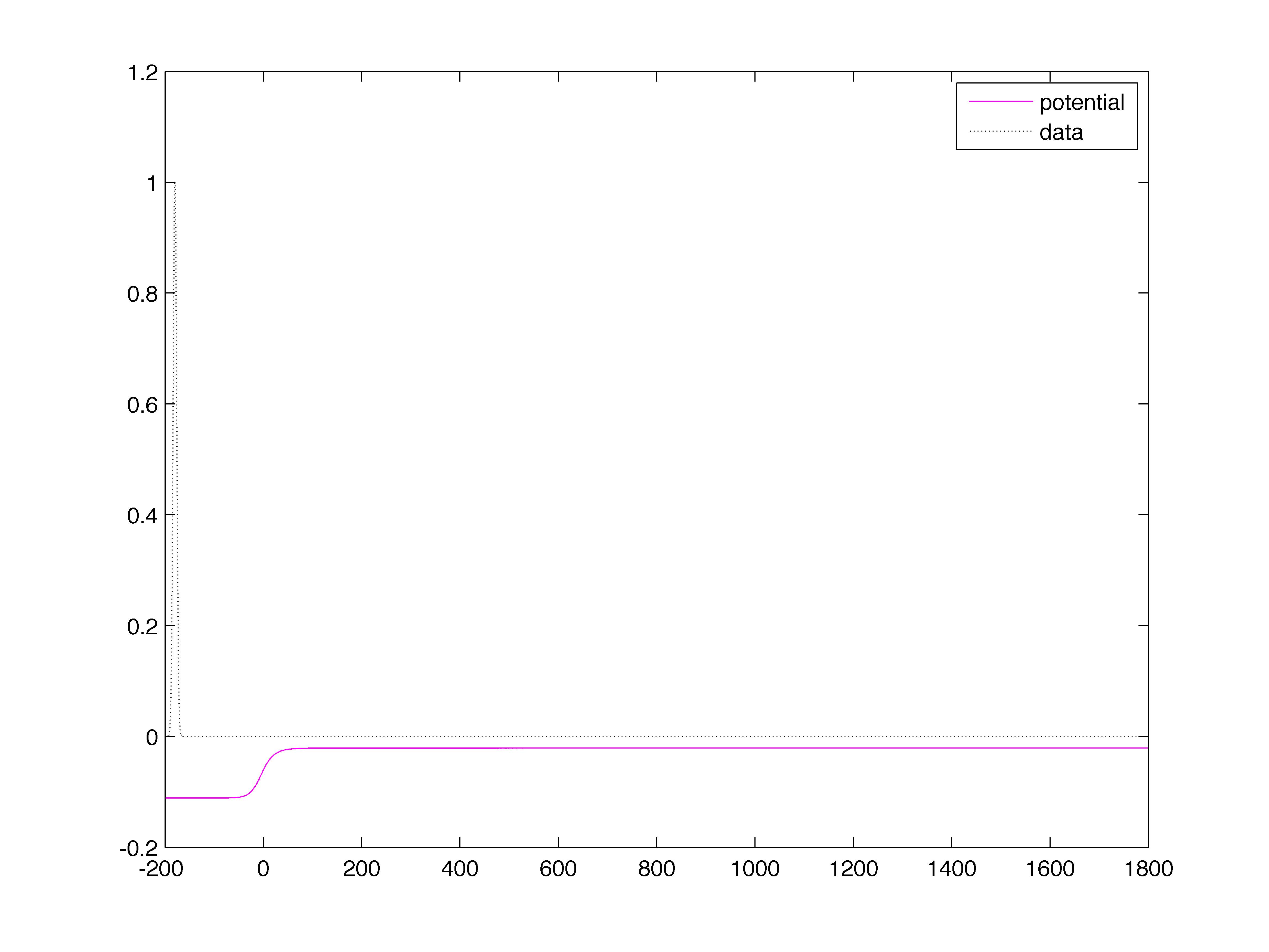
  Figure 10: Data and potential.

  

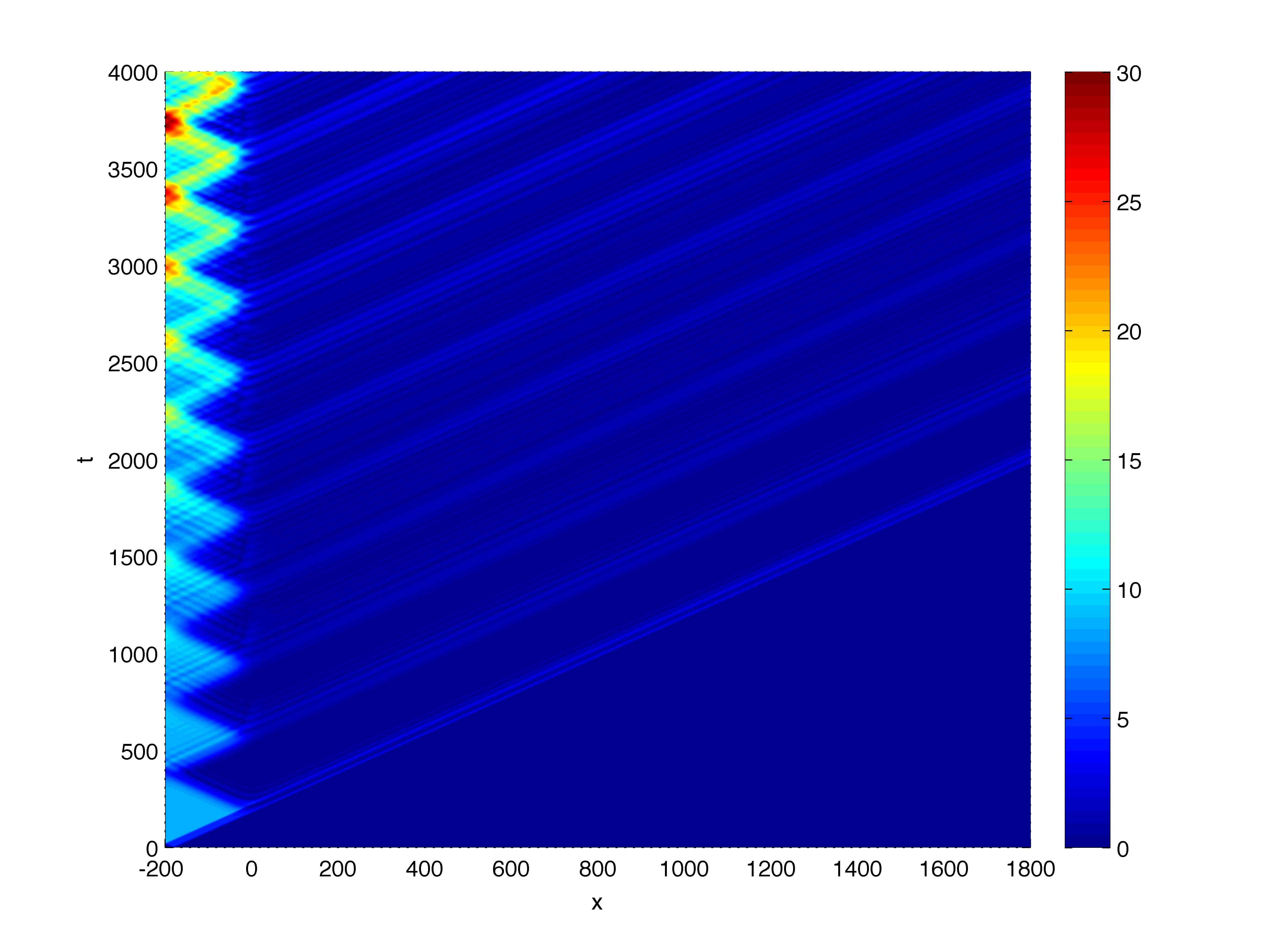
  Figure 11: $(x,t)$ Isovalues of the solution.

  

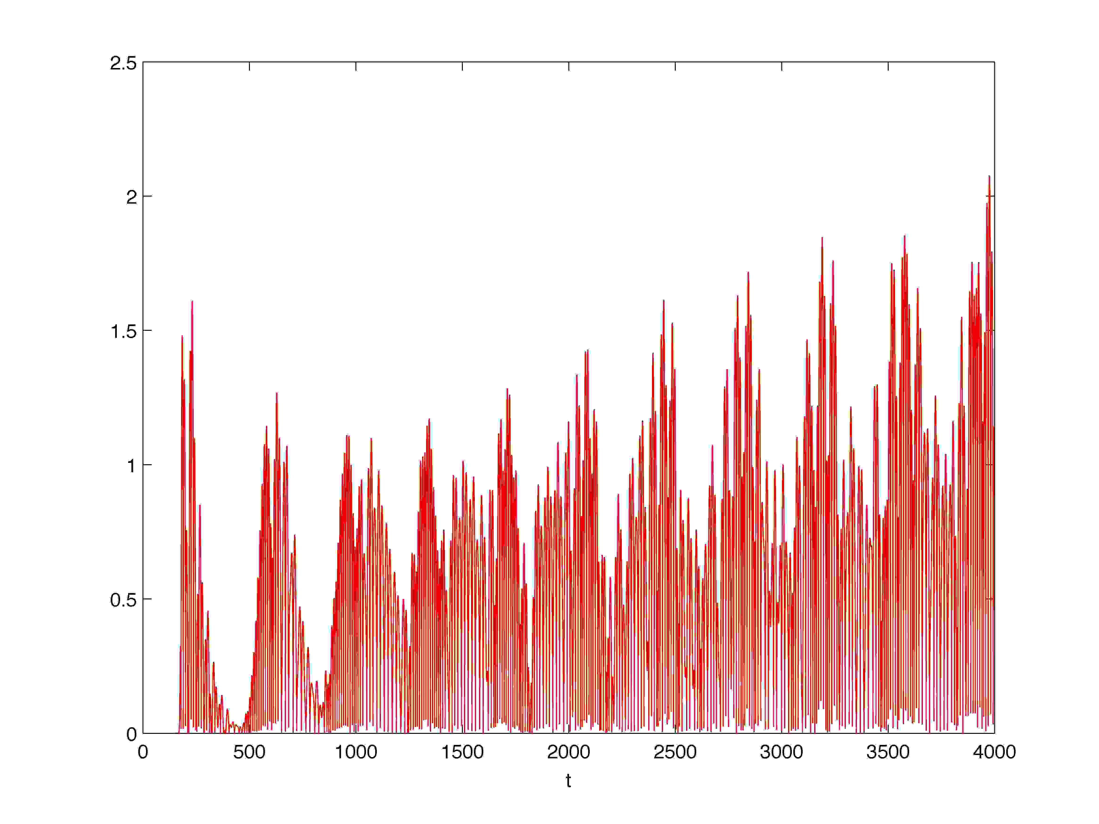
  Figure 12: Profile of the logarithm of the amplitude, $m=0.1$.

  

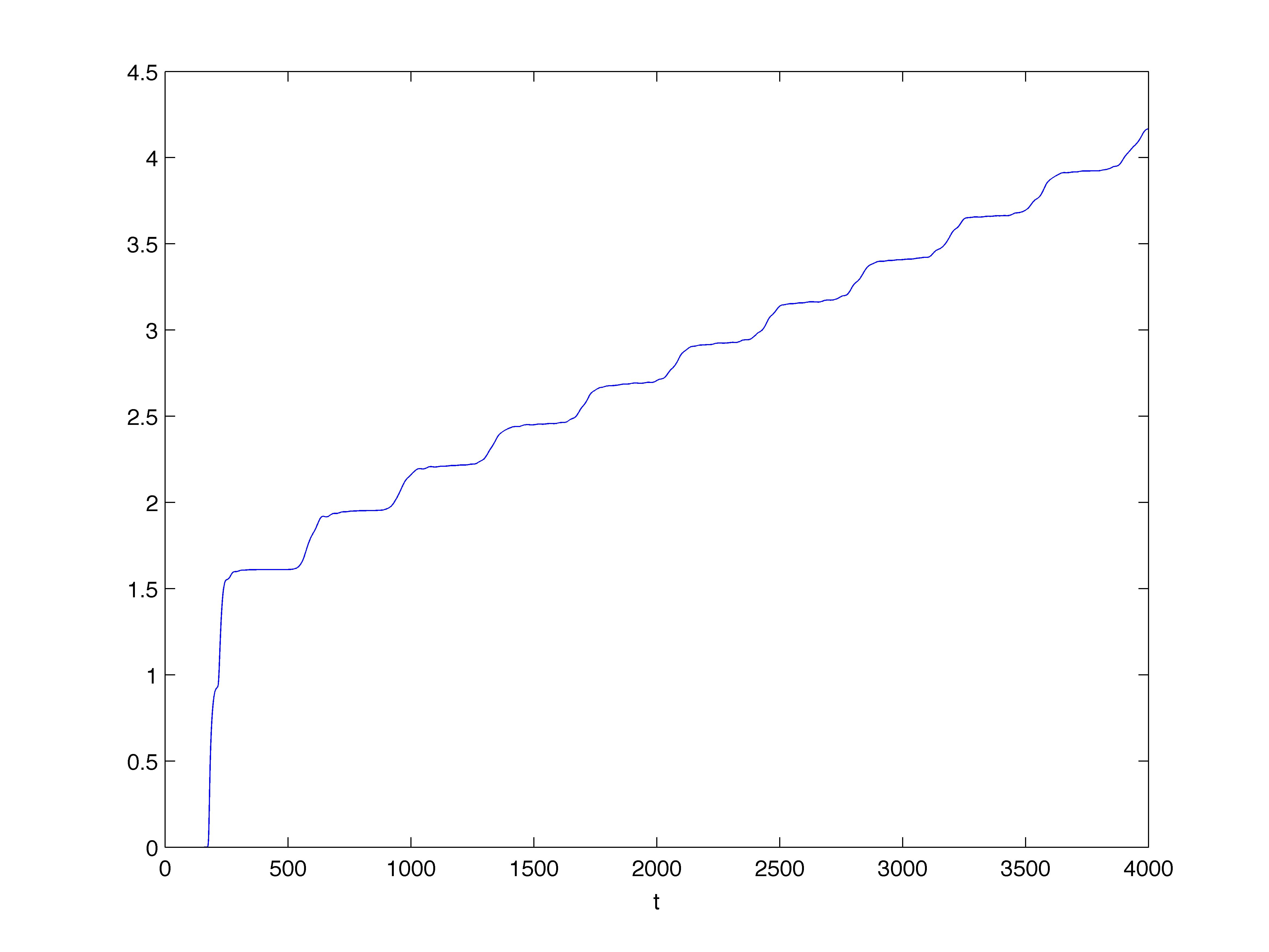
  Figure 13: Profile of the logarithm of the energy gain, $m=0.1$.

  

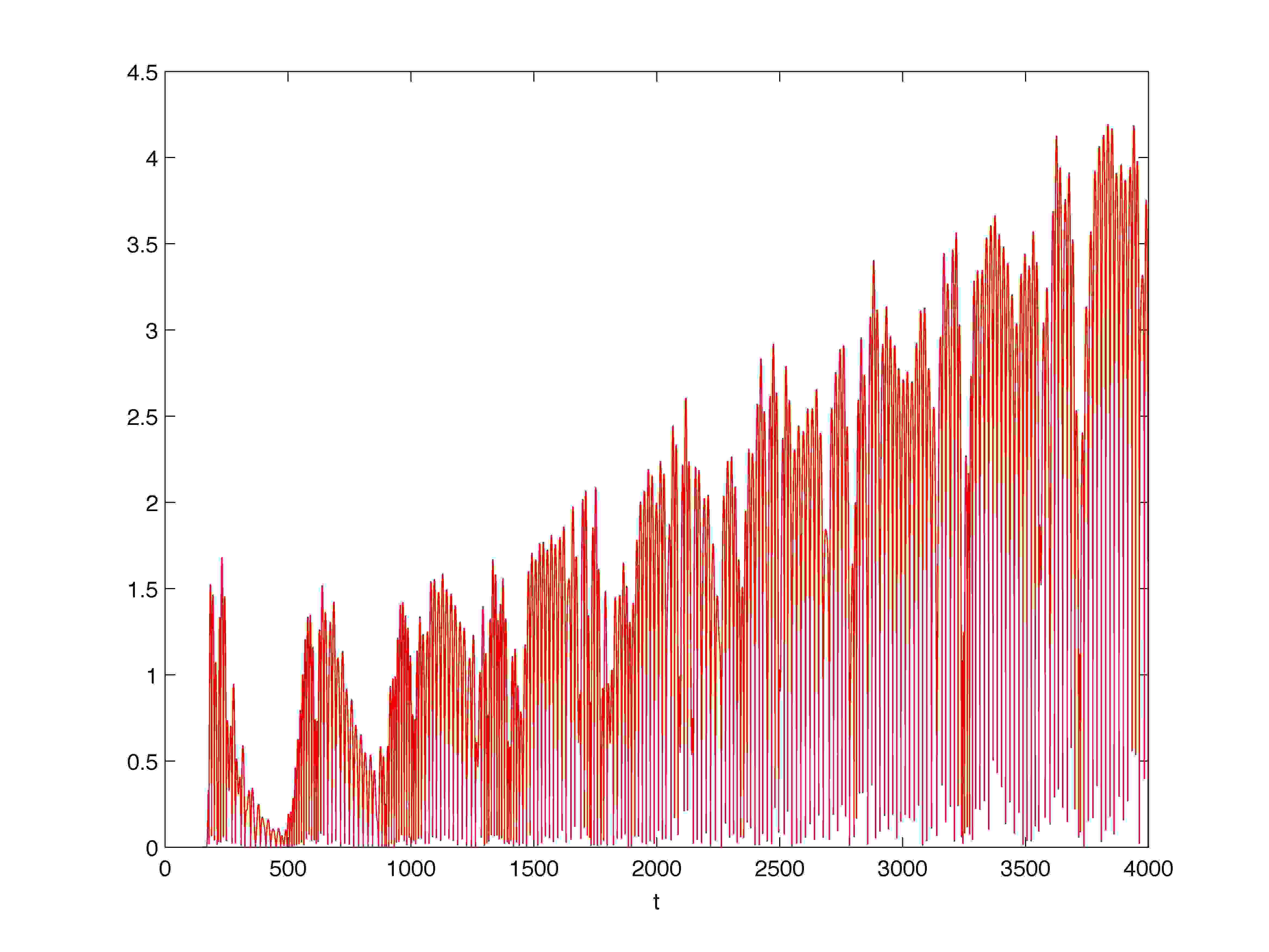
  Figure 14: Profile of the logarithm of the amplitude, $m=0$.

  

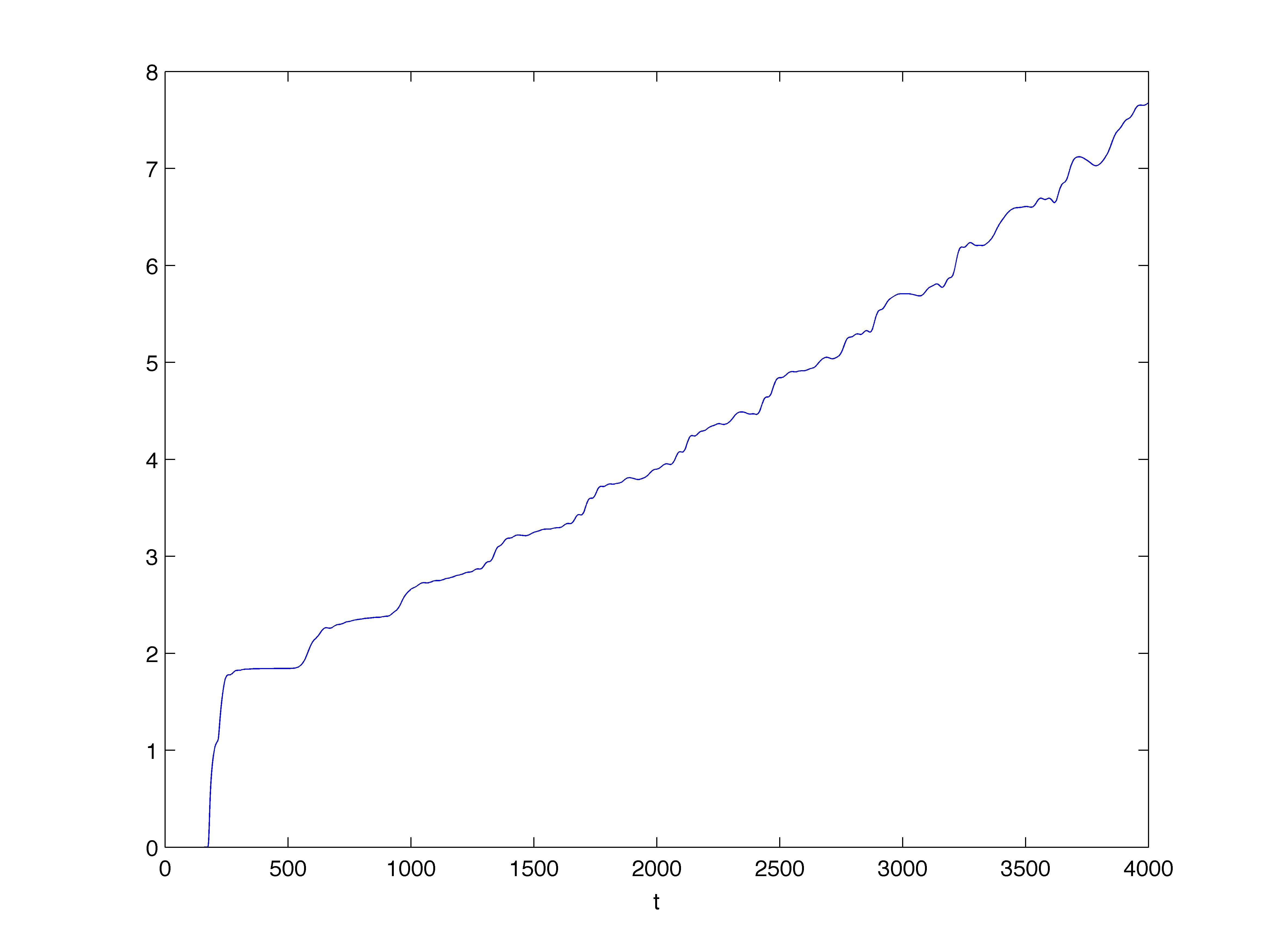
  Figure 15: Profile of the logarithm of the energy gain, $m=0$.

The parameters of the field are $m=0.1$, $q=1$, and $l=0$ (the solution is spherically symmetric). We work on the spatial domain $[-200,1800]$ which is entirely contained inside the ergoregion. We discretise it with $10000$ points and perform simulations with Neumann homogeneous boundary conditions up to $T=4000$ with $\delta t=h$. The data are given by (33) with $\alpha=5$, $x_{0}=-180$, and $\omega=0$. The amplitude of the field and the outgoing energy gain are measured at $x=0$. The data and the potential are displayed in Figure 11. We see that the potential undergoes a sharp transition between two approximately constant regimes, but the size of the jump is fairly small. The evolution in Figure 11 shows that the field bounces between the mirror and the potential barrier, each reflection of the barrier being accompanied by a burst being sent to infinity. The amplitude of the field appears to grow exponentially (see Figure 13) but with a small coefficient, which is likely due to the small size of the barrier. The outgoing energy gain displays a faster exponential growth (Figure 13). The growth is slower than in the asymptotically flat case. Considering a massless field with all the other parameters unchanged, we observe in Figures 15 and 15 a steeper exponential growth for both the amplitude of the solution and the energy gain, the behaviour of the field being otherwise very similar. A simulation with Dirichlet boundary conditions shows a similar behaviour, but milder; we do not display it here.

5.2 Black hole bombs of type I

This is the analogue of the Press-Teukolski construction in the spherically symmetric setting, so one feels that one knows what to expect. This is true but we show that depending on the parameters of the field and the black hole, the behaviour can be quantitatively and qualitatively quite different.

• We start with a massless field on a Reissner-Nordstr m background. The parameters of the black hole are $M=2.001$ and $Q=2$ and for the field $q=1$, $m=0$, $l=0$. The potential and data are shown in Figure 16. We see that the potential remains negative on the whole computational domain $[-1700,100]$, which is consequently entirely contained inside the ergoregion. In fact in this situation, the ergoregion covers the whole block III. The final time is $T=3000$, the spatial domain is discretised with $20000$ points and $\delta t=h$. Our initial data is as in (33) with $\omega=0$, $\alpha=5$, and $x_{0}=20$. The measure of the outgoing energy flux and of the amplitude of the solution are done at $x=55$. Figures 17 and 18 show the evolution of the logarithm of the amplitude and the energy gain for both Neumann and Dirichlet boundary conditions. The phenomenon is a mirror image of what we observed for type II bombs in the Reissner-Nordstr m case: the field creeps along the mirror with its amplitude growing exponentially in time, bursts of negative energy are sent towards the horizon and positive energy accumulates close to the mirror, growing exponentially as well.

  

  Figure 16: Potential and initial data for $m=0$.

  

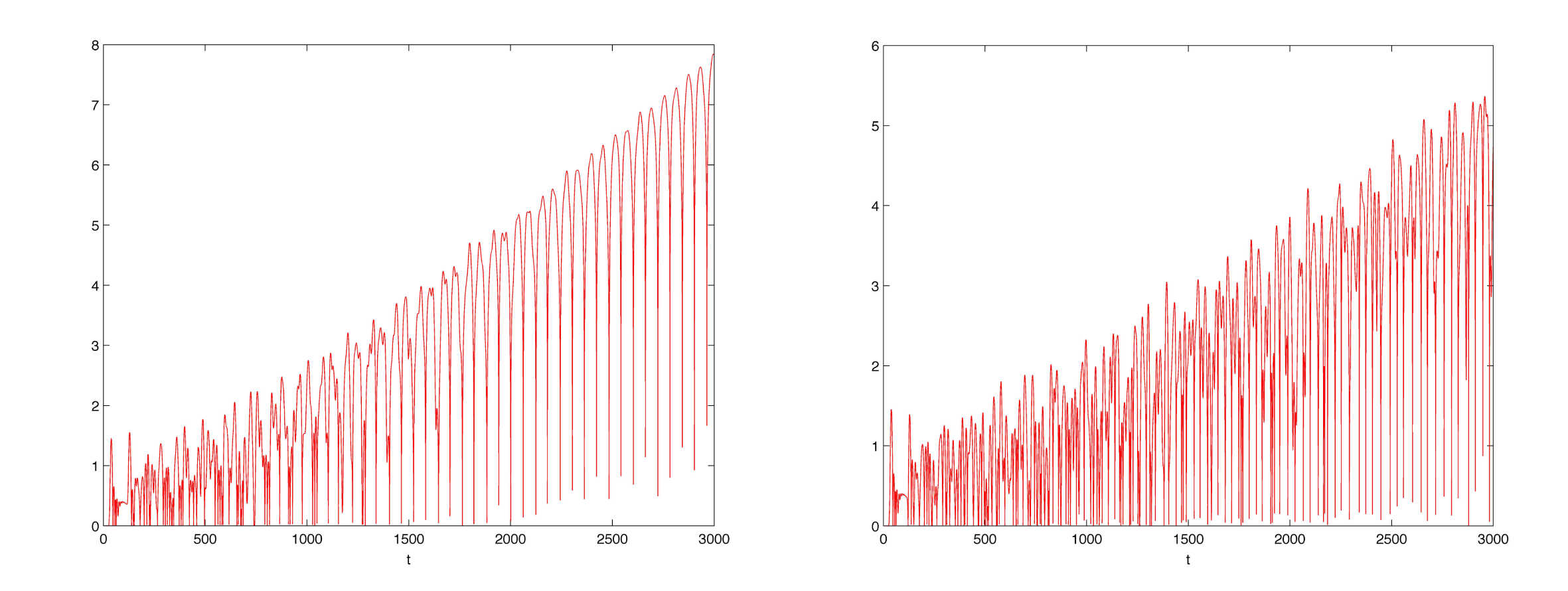
  Figure 17: Profile of logarithm of amplitude: Neumann conditions (left), Dirichlet conditions (right).

  

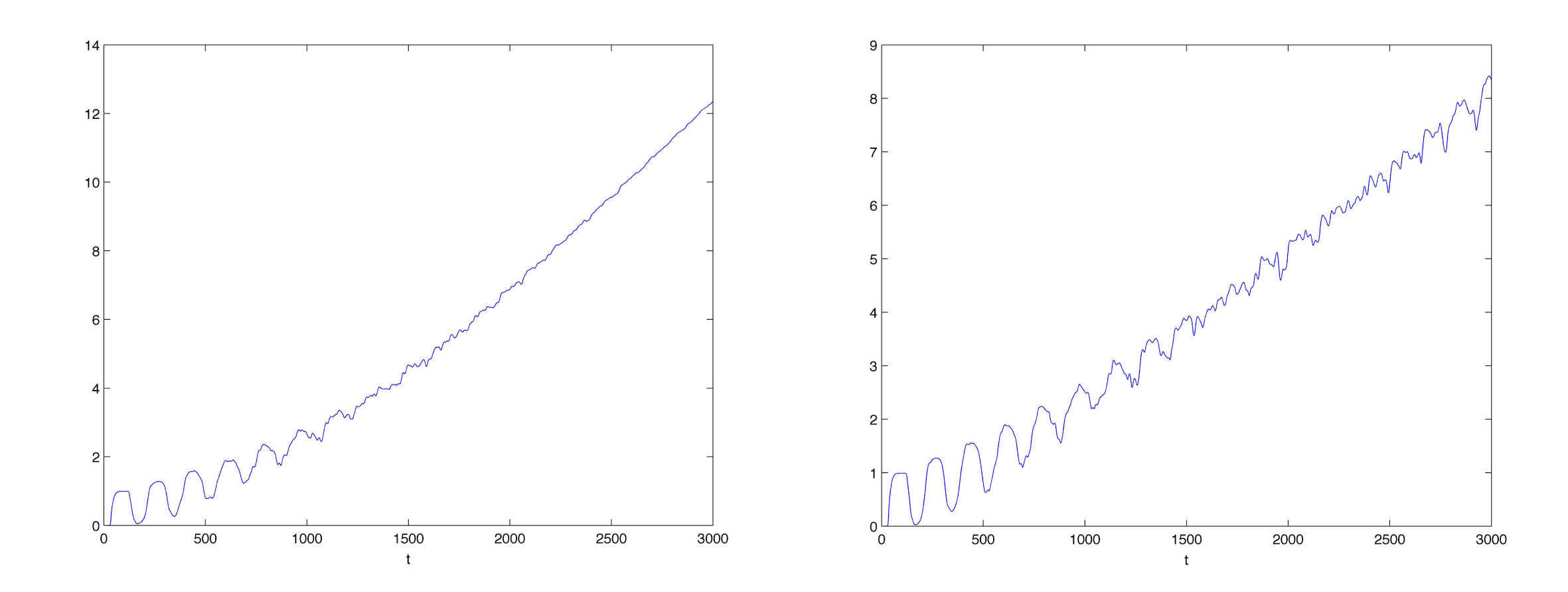
  Figure 18: Profile of logarithm of energy gain: Neumann conditions (left), Dirichlet conditions (right).

• On the same background, we study the evolution of a massive field with small mass $m=0.1$ so as to ensure that there is still superradiance. All the other parameters are the same. Due to the mass of the field, the ergoregion has shrunk and the mirror is now outside of it (see Figure 20). The simulations with Neumann and Dirichlet boundary conditions are almost indistinguishable, we simply display the Neumann case here.

  The isovalues of the solution and the evolution of the logarithm of the amplitude and the energy gain are displayed in Figures 20, 22, and 22. The behaviour of the solution is qualitatively different. A part of the field stays confined between the mirror and the boundary of the ergoregion and bounces back and forth between the two. The reflection does not actually happen at the frontier of the ergoregion, but a little inside and it mimicks a Penrose process: the field enters the ergoregion, splits spontaneously into a part that has negative energy and falls into the black hole, and a part that has positive energy and tries to escape to infinity, but is prevented to do so by the mirror. This is a similar phenomenon to what was observed in Ref. [10] but here it occurs repeatedly due to the presence of the mirror. We see from Figure 22 that the oscillations in the logarithm of the energy gain grow linearly, which suggests that at each occurrence of the Penrose process, the same fraction of the energy of the incoming field is extracted from the ergoregion, causing an exponential accumulation of energy between the ergoregion and the mirror. The amplitude of the field also appears to grow exponentially, but this is a much milder growth than in the massless case.

  

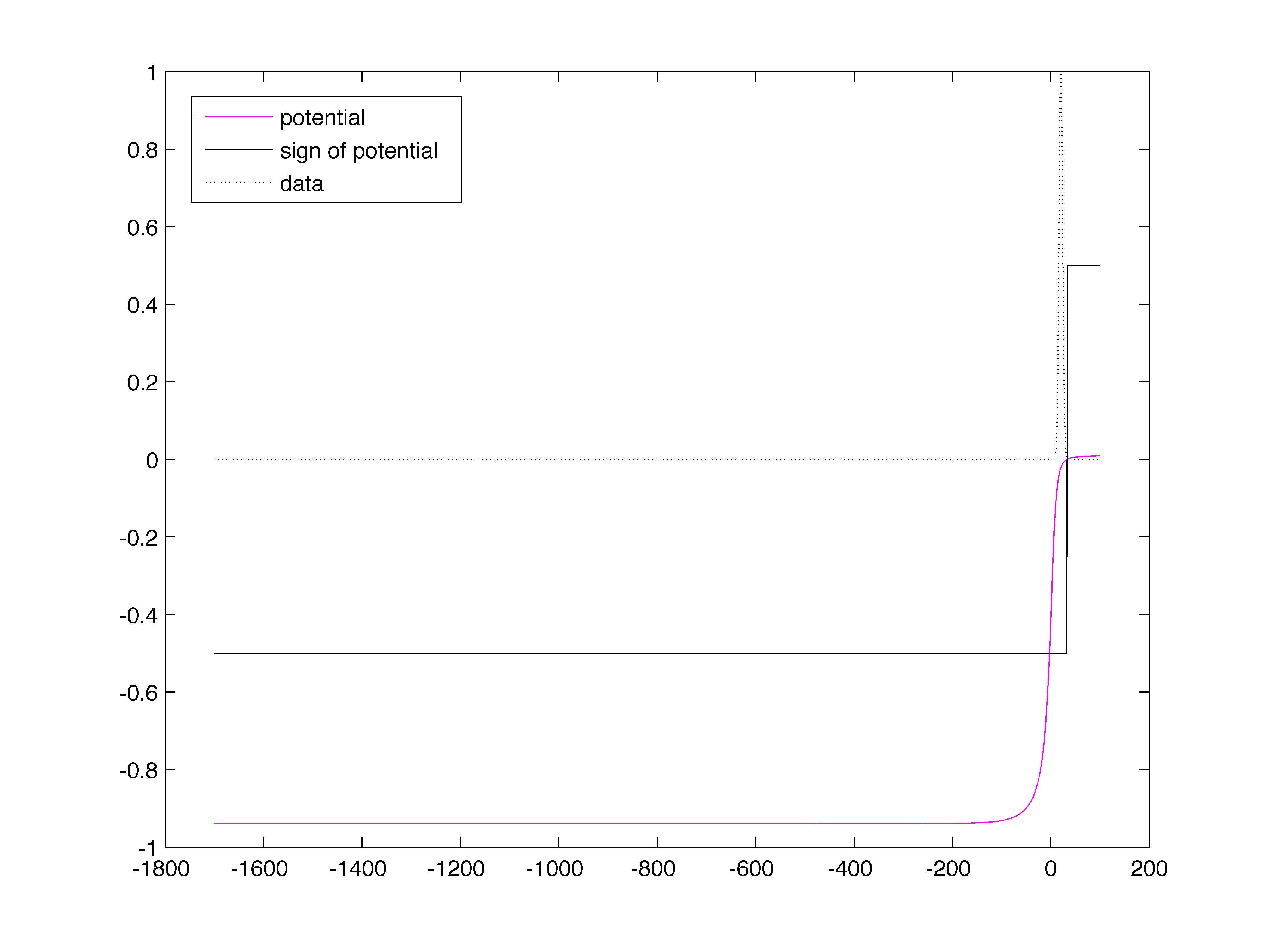
  Figure 19: Potential and initial data for $m=0.1$.

  

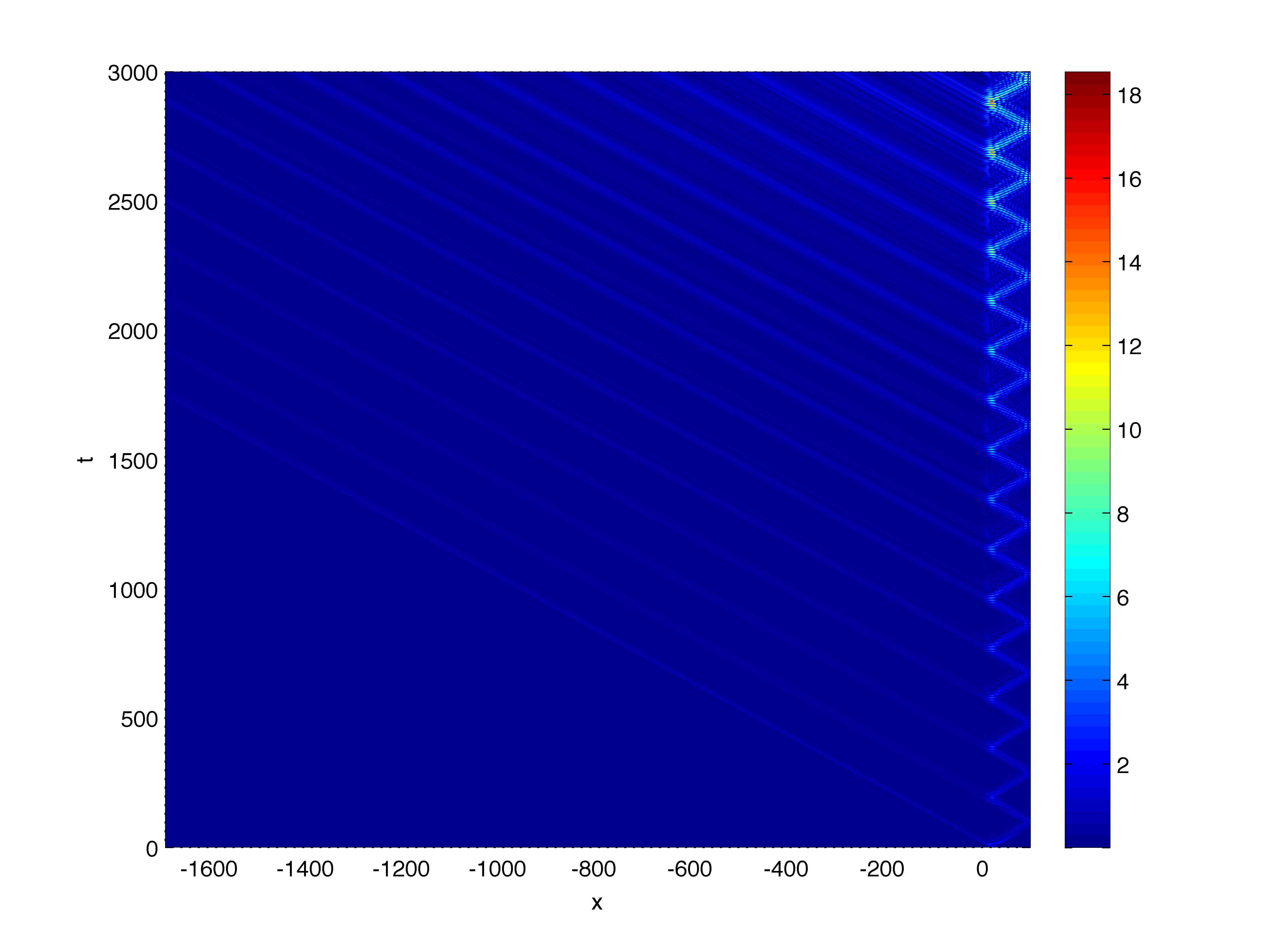
  Figure 20: $(x,t)$ isovalues of the solution, $m=0.1$.

  

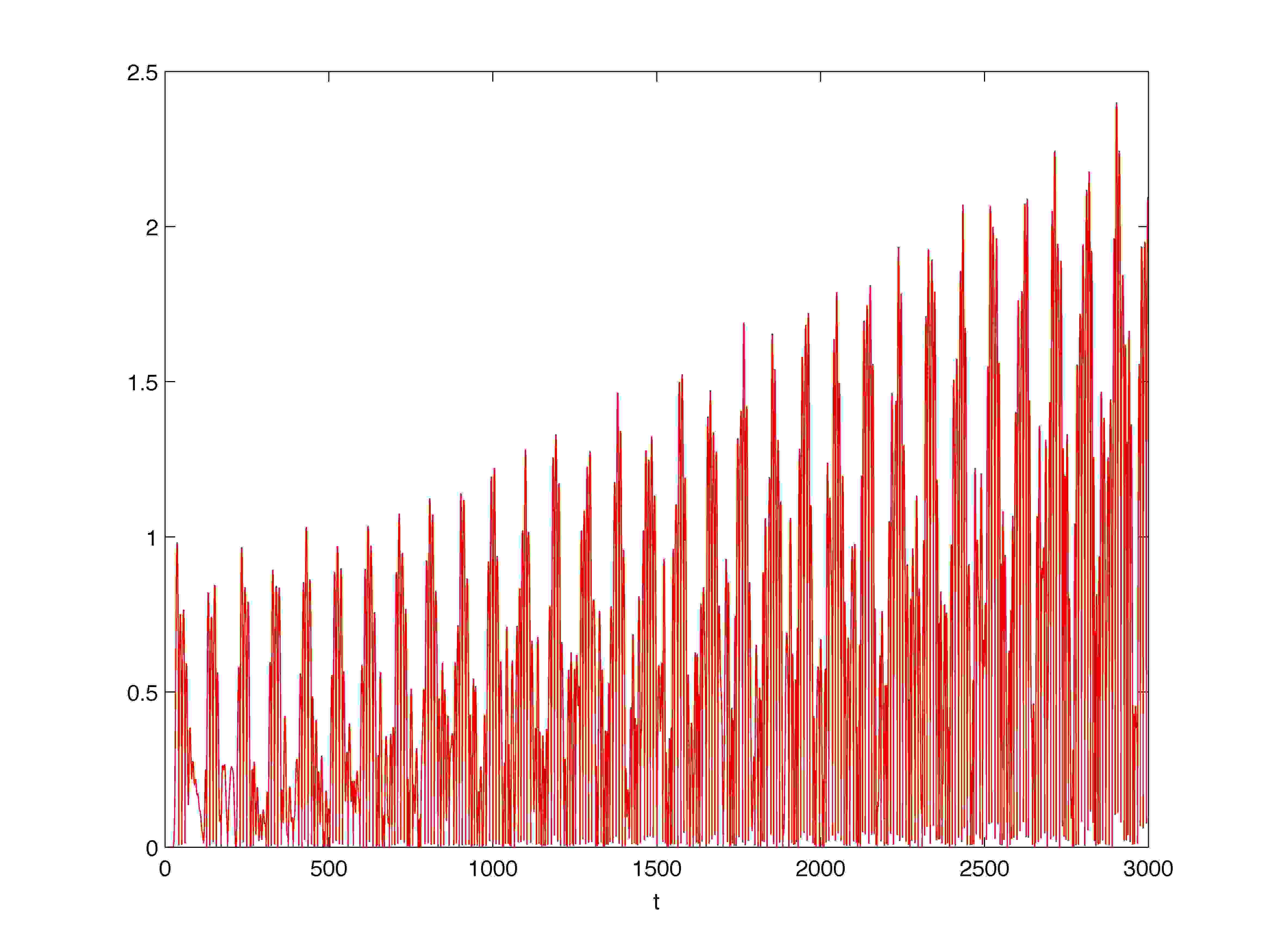
  Figure 21: Profile of the logarithm of the amplitude in the massive case.

  

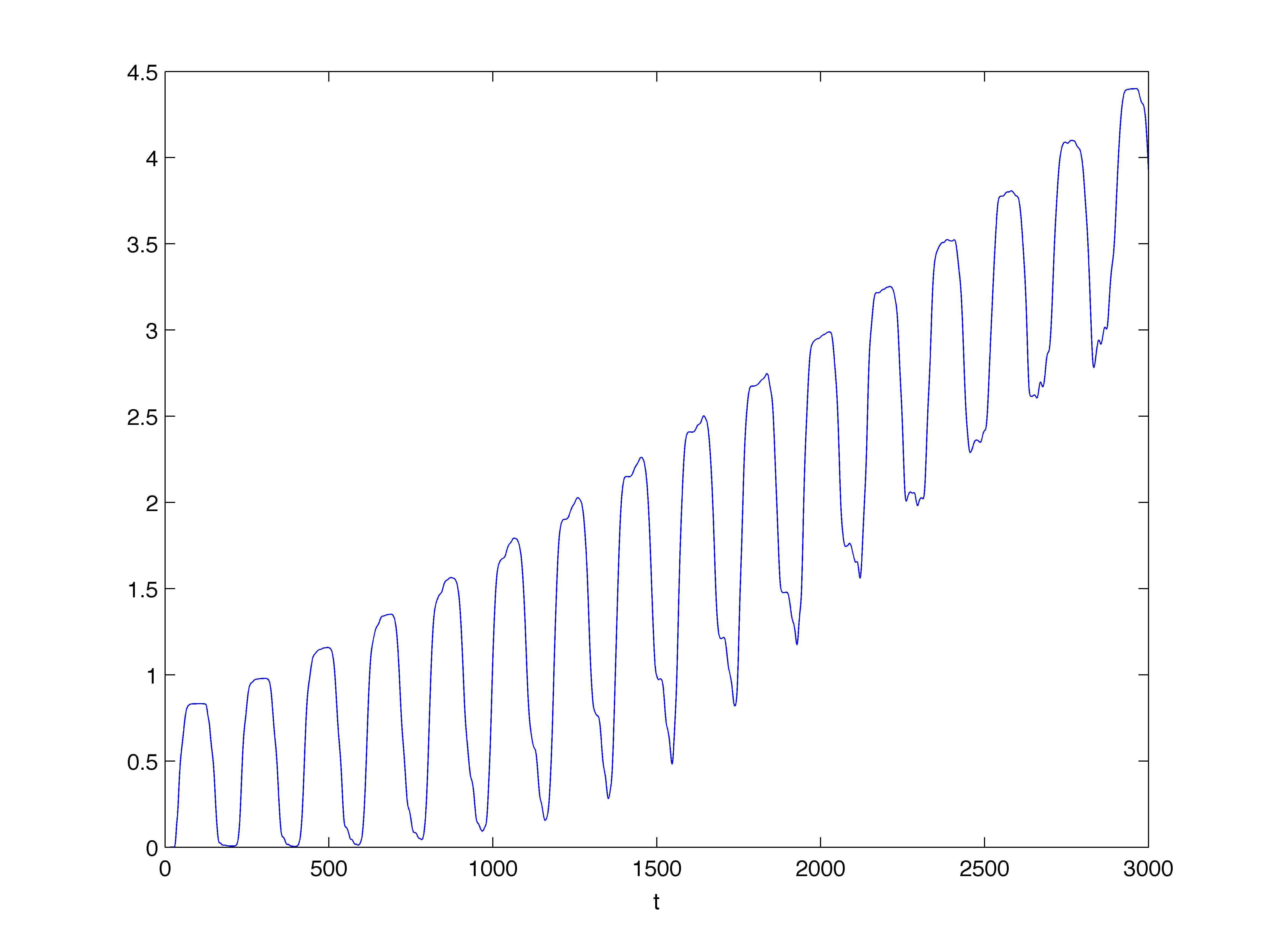
  Figure 22: Profile of the logarithm of the energy gain in the massive case.

• We conclude this section on type I bombs with a study of the behaviour of a massless field outside a de Sitter Reissner-Nordstr m black hole with the same parameters as before: $Q=2$, $M=3$, and $\lambda=1/(6M)^{2}$. The final simulation time has been taken equal to $T=2000$ on the domain $[-900,100]$ discretised with $10000$ spatial points, with $\delta t=h$. The flare-type Cauchy data is centred at $x_{0}=-100$ with $\alpha=5$ and $\omega=0$. The amplitude of the solution and the outgoing energy flux are measured at $x=0$. Figure 23 displays a potential with a sharp jump but of small magnitude. The field being massless, we nevertheless observe in Figures 24 and 25 a clearcut exponential growth of the amplitude and the outgoing energy gain. In the case of Dirichlet boundary conditions, the growth is milder than for Neumann conditions.

  

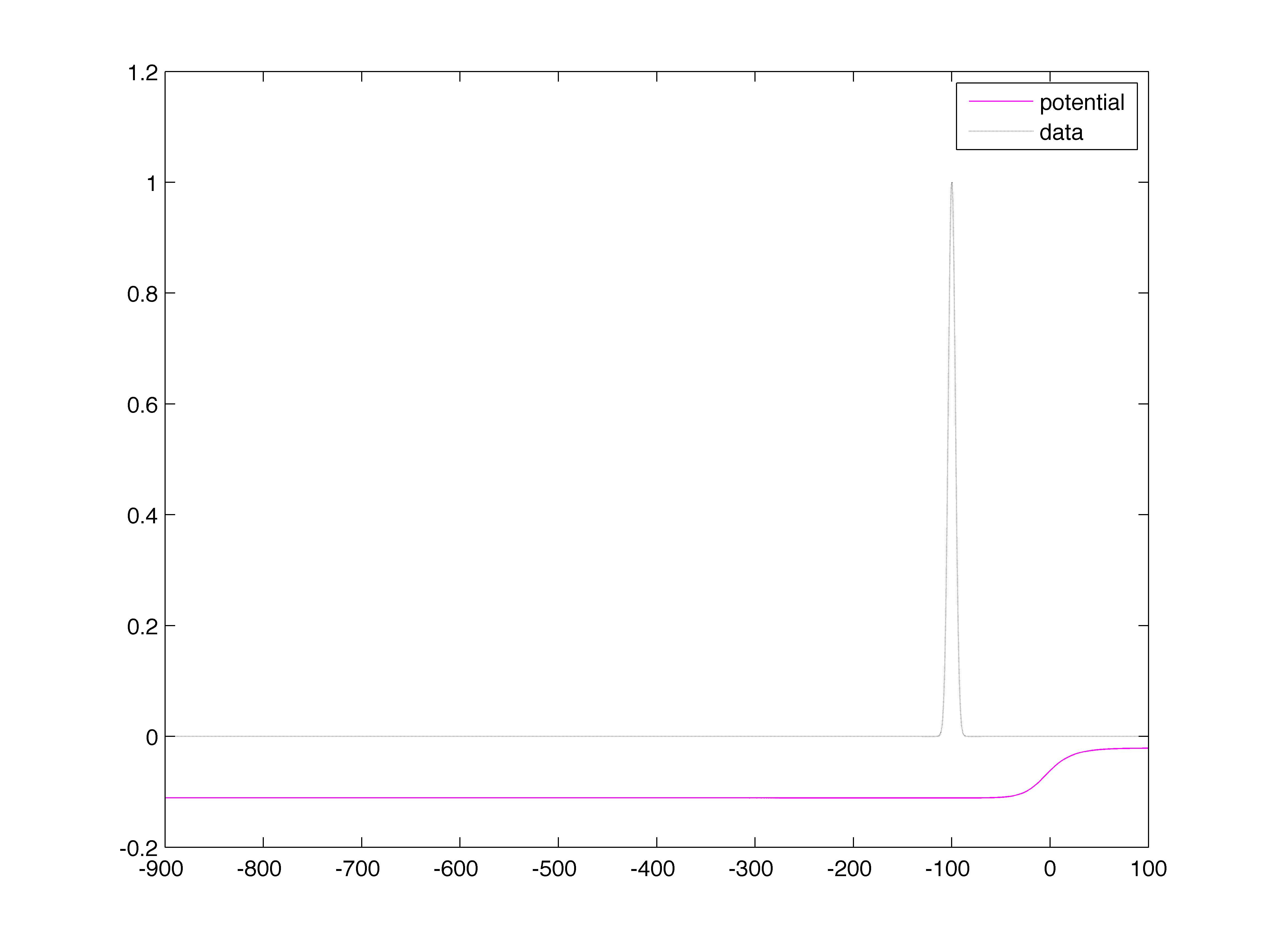
  Figure 23: Data and potential.

  

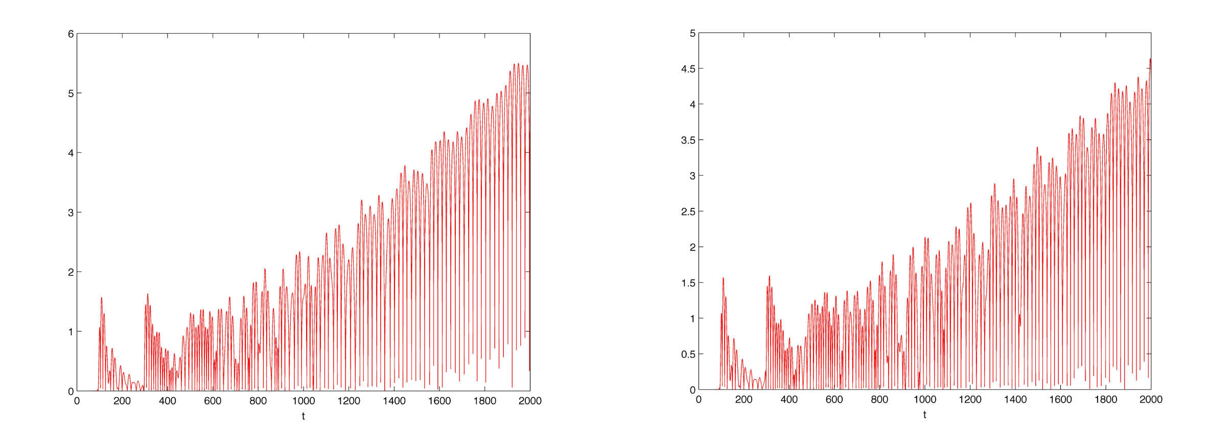
  Figure 24: Profile of logarithm of amplitude: Neumann conditions (left), Dirichlet conditions (right).

  

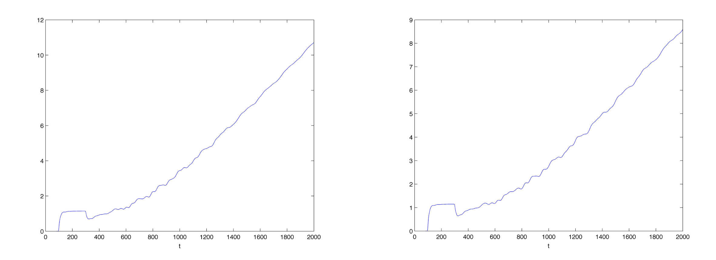
  Figure 25: Profile of logarithm of energy gain: Neumann conditions (left), Dirichlet conditions (right).

5.3 Black hole bombs of type III

We study these sandwich bombs on the two types of backgrounds studied previously.

• The first test is performed outside a Reissner-Nordstr m black hole of mass $M=2.5$ and charge $Q=2$, for a field of mass $m=0.1$, angular momentum $l=0$, and charge $q=1$. The computational domain is $[-40,40]$ discretised with $6000$ points. The initial data are of the form (33) with scaling factor $\alpha=5$, $x_{0}=-20$, $\omega=0$. The amplitude and outgoing energy flux are measured at $x=0$. For Neumann boundary conditions, the calculations are performed up to $T=1500$. For Dirichlet conditions, the growth is slower and we push the calculation to $T=2000$ with $8000$ points in order to observe something conclusive.

  

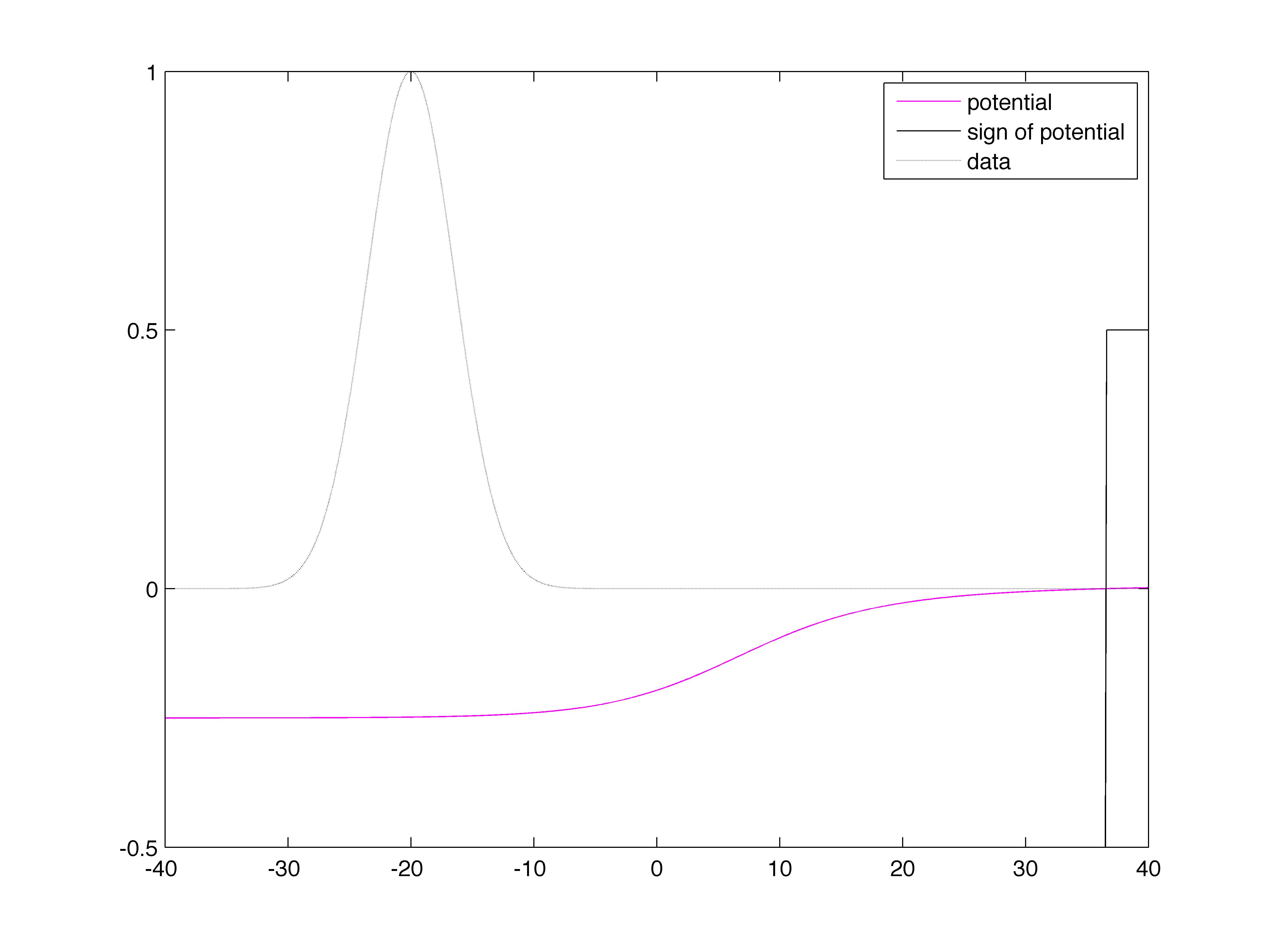
  Figure 26: Data and potential.

  

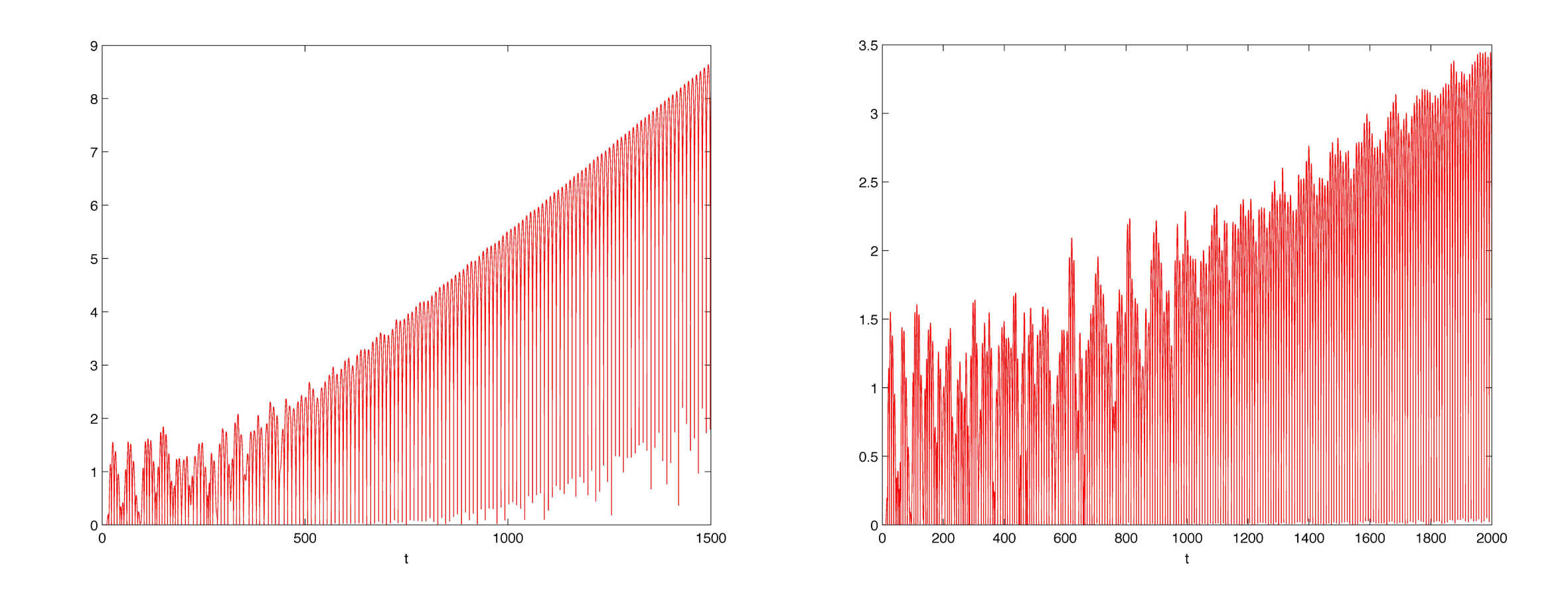
  Figure 27: Profile of logarithm of amplitude: Neumann conditions (left), Dirichlet conditions (right).

  

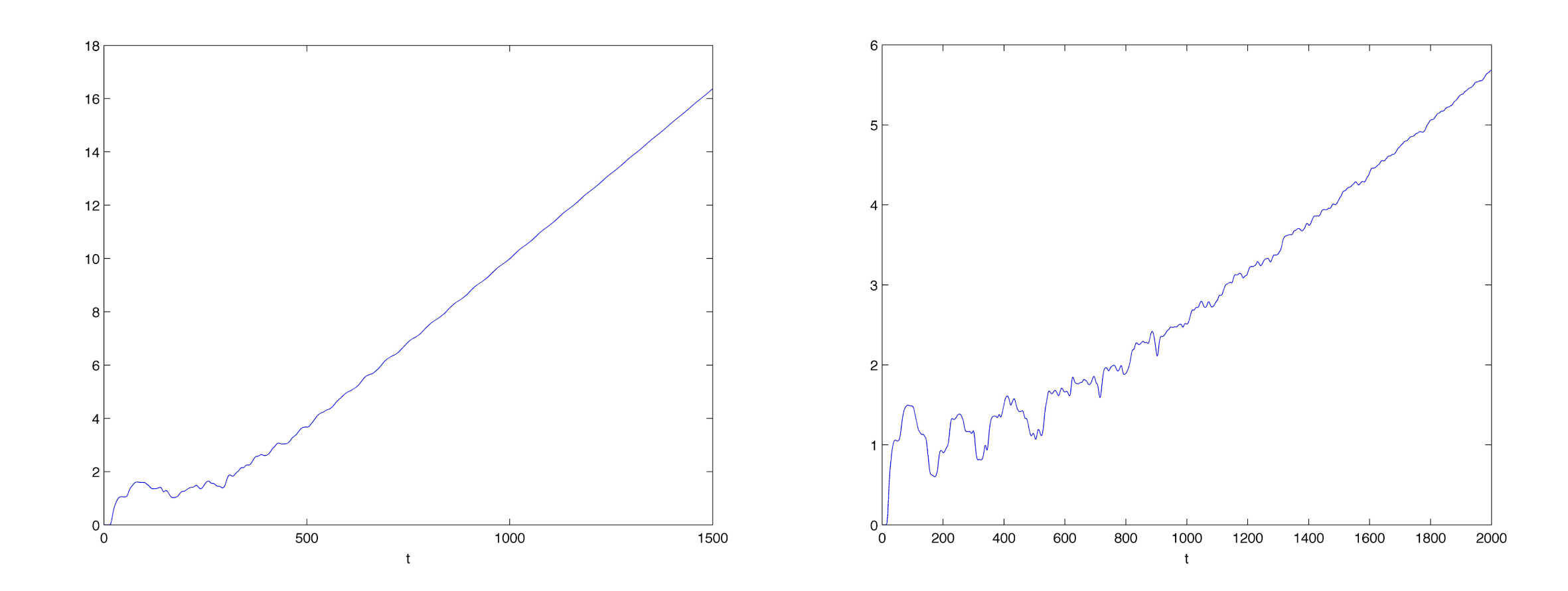
  Figure 28: Profile of logarithm of energy gain: Neumann conditions (left), Dirichlet conditions (right).

  We note (Figure 26) that the potential is negative on the left-hand side of the domain and changes sign near the outer mirror. Its transition is rather mild; with incoming wave packets, this would make it difficult to observe superradiance, but with flares, superradiant behaviour is more easily captured. The amplitude of the field as well as the energy gain increase exponentially (Figures 27 and 28), the latter meaning that negative energy accumulates near the inner mirror and positive energy near the outer mirror, at an exponential rate.

• We also consider the de Sitter-Reissner-Nordstr m black hole that we have considered before, with $Q=2$, $M=3$, and $\lambda=1/(6M)^{2}$. The spatial domain is $[-40,40]$ with $4000$ discretisation points and we perform our simulation up to time $T=1000$ with $\delta t=h$.

  

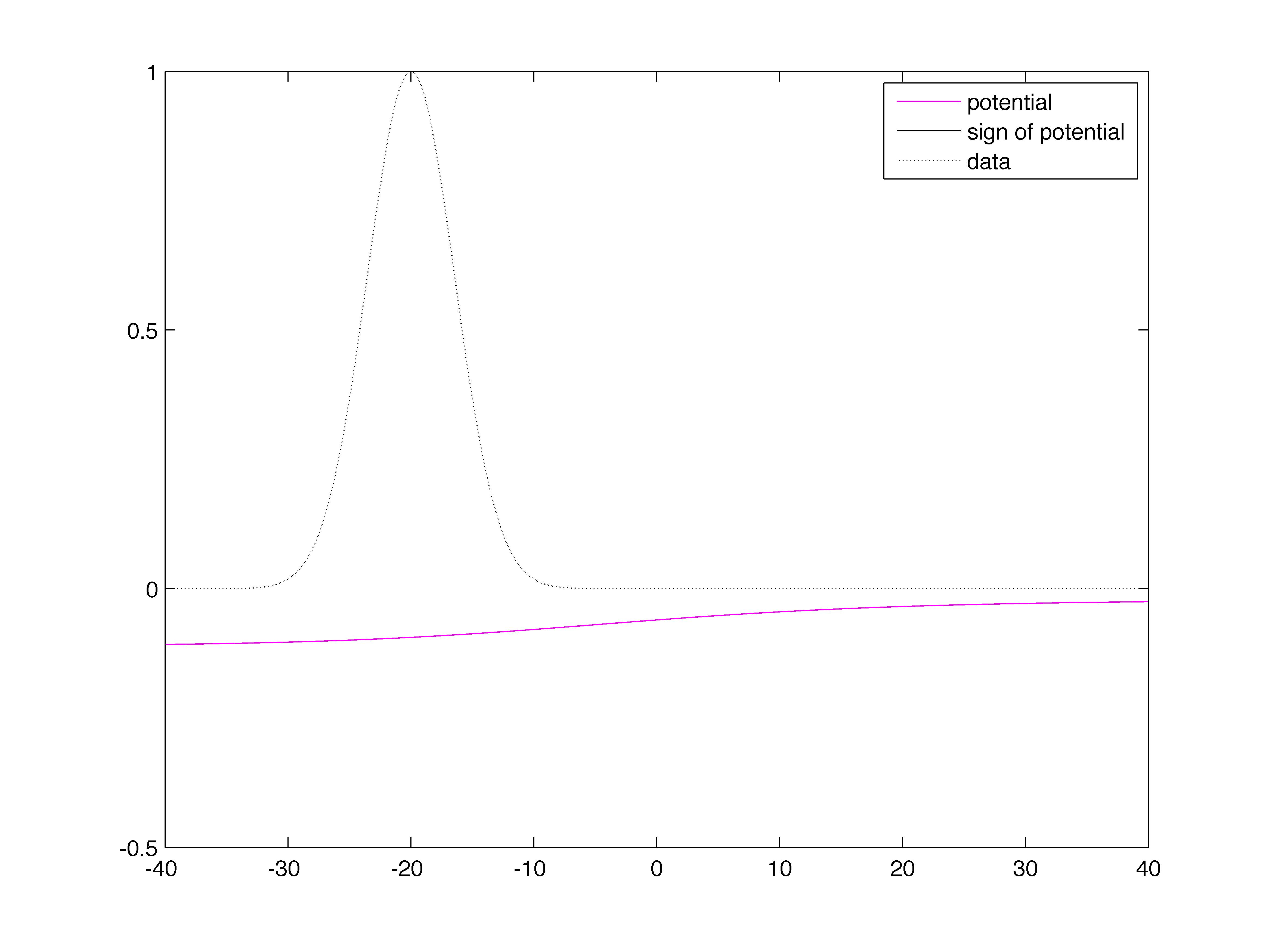
  Figure 29: Data and potential, $q=1$.

  

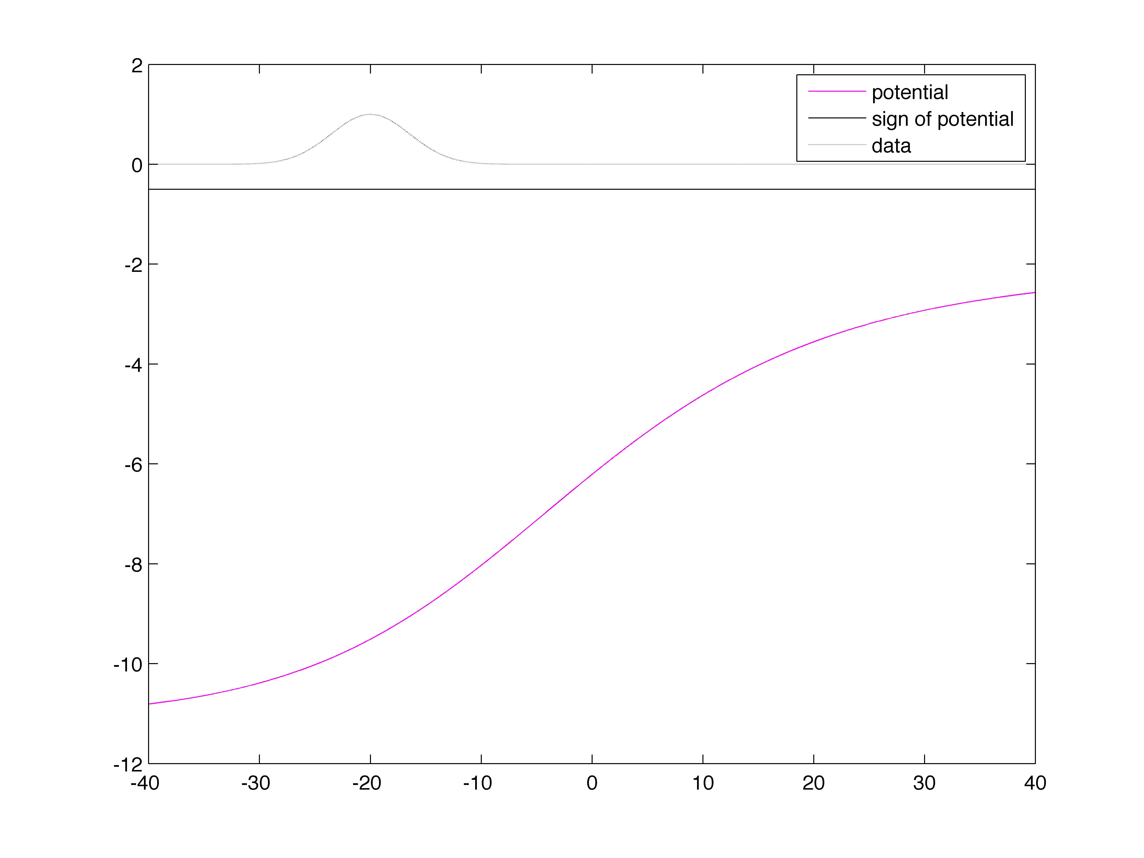
  Figure 30: Data and potential, $q=10$.

  

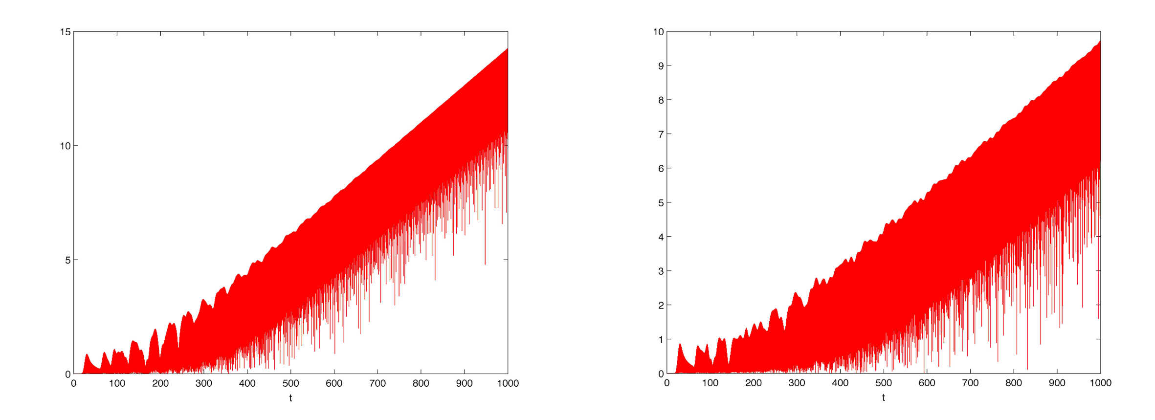
  Figure 31: Profile of logarithm of amplitude: Neumann conditions (left), Dirichlet conditions (right).

  

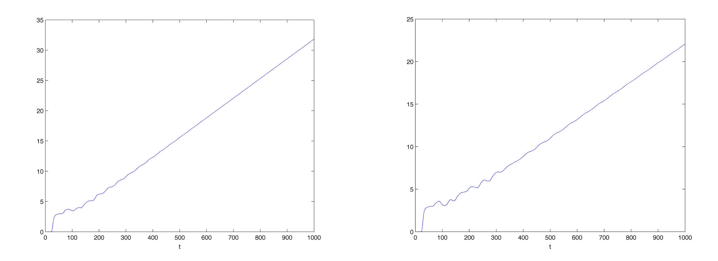
  Figure 32: Profile of logarithm of energy gain: Neumann conditions (left), Dirichlet conditions (right).

  First, we try a field with mass $m=0.1$, $l=0$, $q=1$ with data given by (33) with $\alpha=5$, $x_{0}=-20$ and we measure the amplitude of the solution and the energy gain at $x=0$. The transition of the potential is extremely mild in this case (Figure 30) and even for large times we do not observe any linear instability. If we increase brutally the charge of the field to $q=10$, we observe a dramatic change and a severe linear instability appears (Figures 31 and 32); the data and potential are displayed in Figure 30.

• Finally, we show an example of high frequency behaviour of our scheme.

  

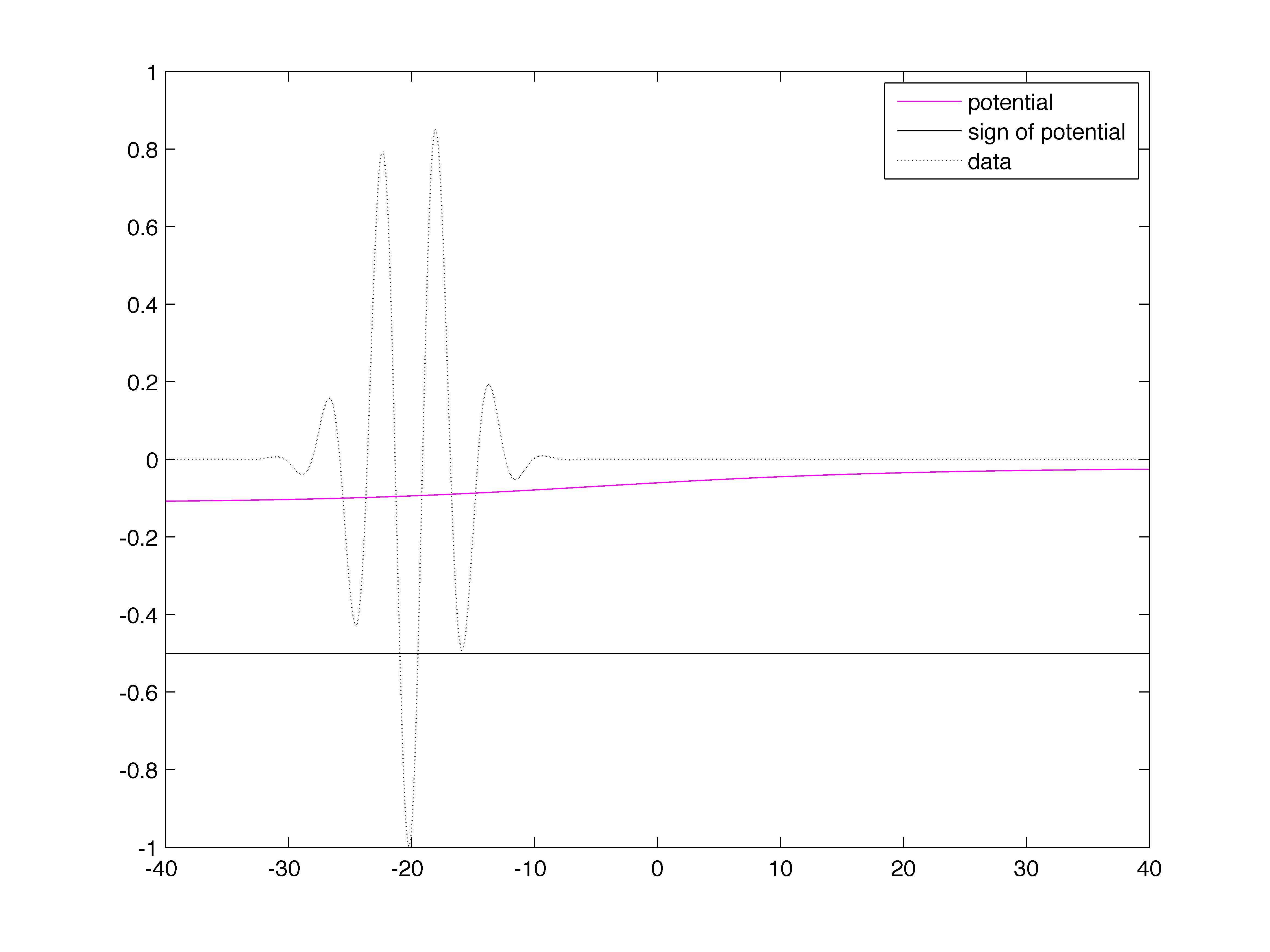
  Figure 33: Data and potential, $q=1$.

  

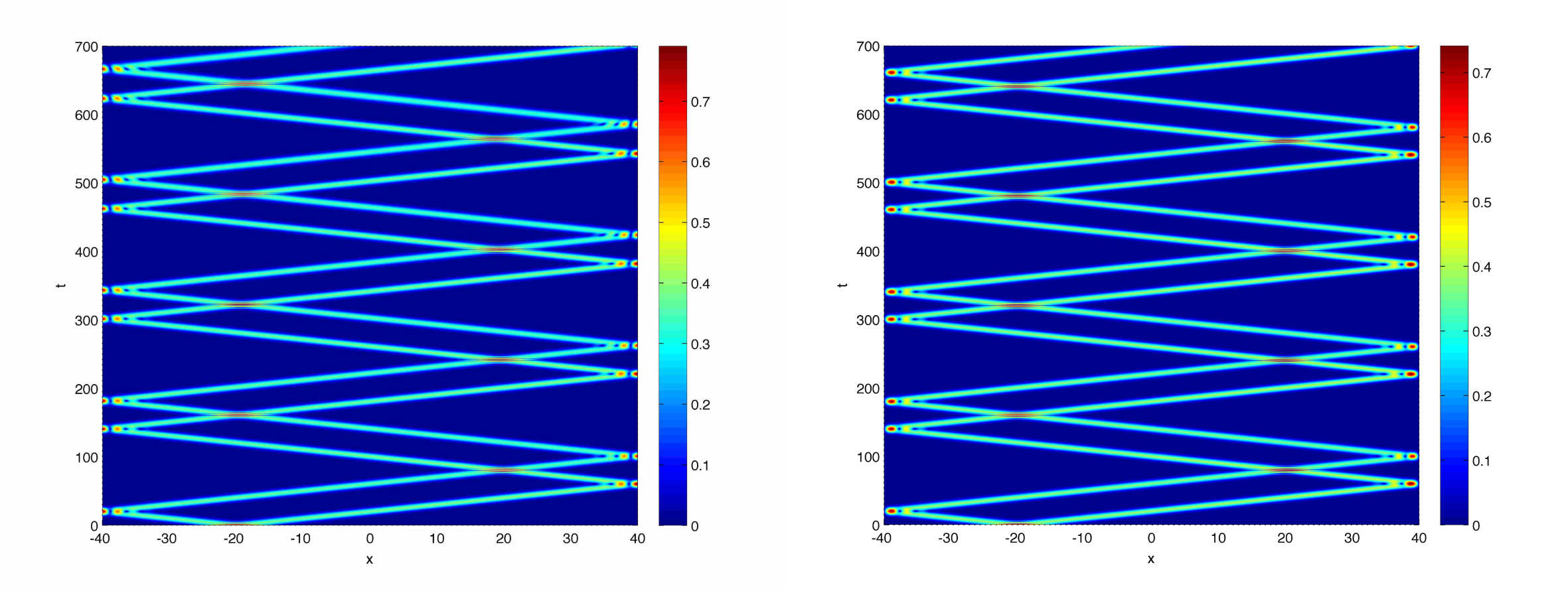
  Figure 34: $(x,t)$ isovalues, high frequency: Neumann conditions (left), Dirichlet conditions (right).

  

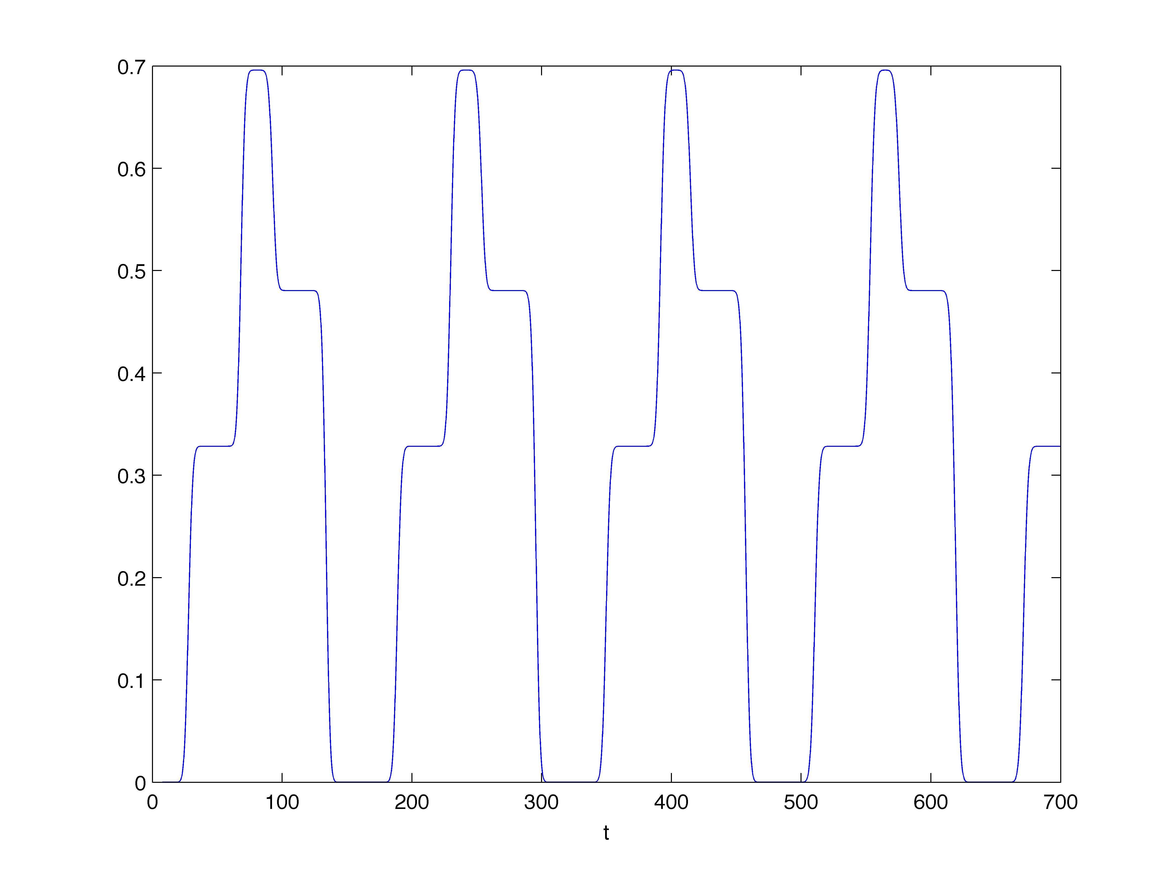
  Figure 35: Profile of log of energy gain, $q=10$.

  We keep the same parameters as in the last simulation with $q=1$, taking now $\omega=7$. The data, the isovalues of the solution, and the profile of the logarithm of the energy gain are displayed in Figures 33, 34, and 35. For the isovalues, we show the simulations with Neumann and Dirichlet conditions; the corresponding energy gain profiles are almost identical and we only display the output for Neumann conditions. The solution follows radial null geodesics between its reflections against the mirrors, no superradiance occurs and the field remains bounded.

5.4 Numerical energy conservation

As was remarked earlier on, the new form of the discrete energy that we have obtained, for both Dirichlet and Neumann boundary conditions, is conserved when considering the exact solution of the numerical scheme. However, the computed solution is only an approximate solution of the scheme and the discrete energy may not be exactly conserved. Moreover, since we are observing a regime in which the solutions display linear instabilities, the small errors made when computing the approximate solution will build up and we have to expect an exponential divergence between the exact discrete solution and the computed one. This must affect the discrete energy and cause exponential divergence. We study the evolution of the discrete energy for the type II black hole bomb on a Reissner-Nordstr m background that we investigated above, with Dirichlet boundary conditions. The simulation is pushed up to $T=1500$ with $16000$ points, then $32000$ and finally $64000$.

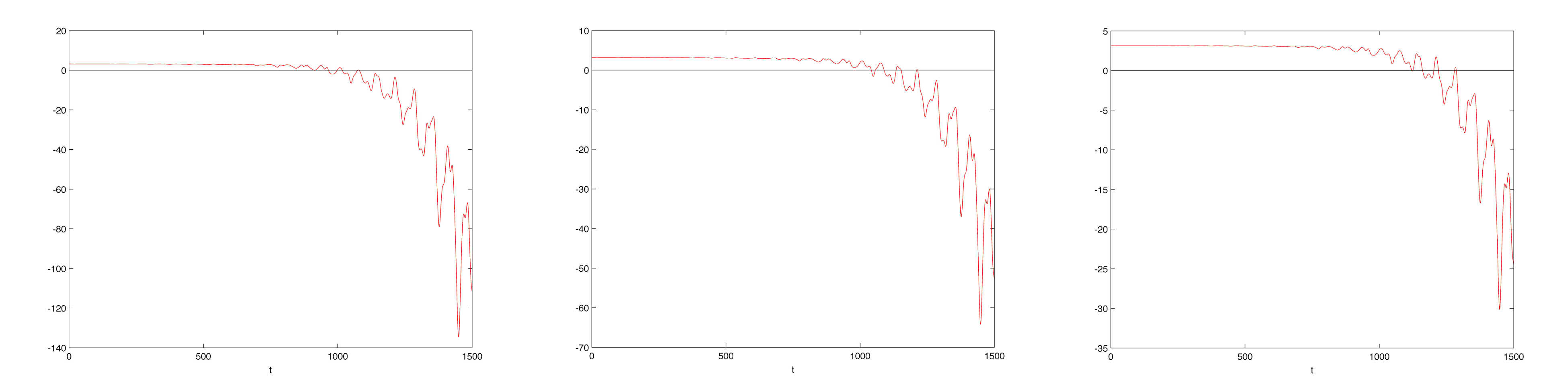
Figure 36: Evolution of the discrete energy, $16000$ points, then $32000$ and $64000$.

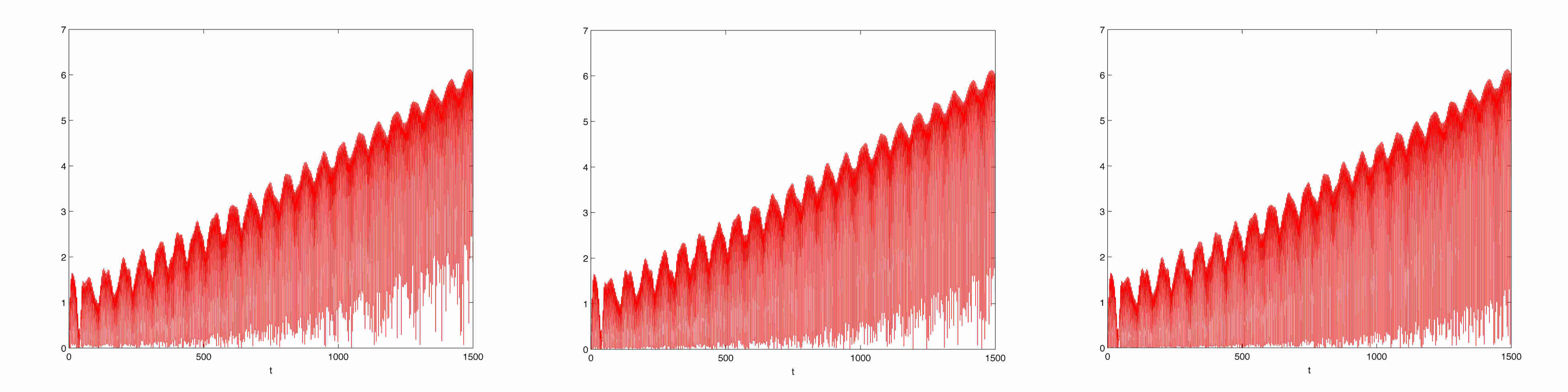
Figure 37: Evolution of the field amplitude, $16000$ points, then $32000$ and $64000$.

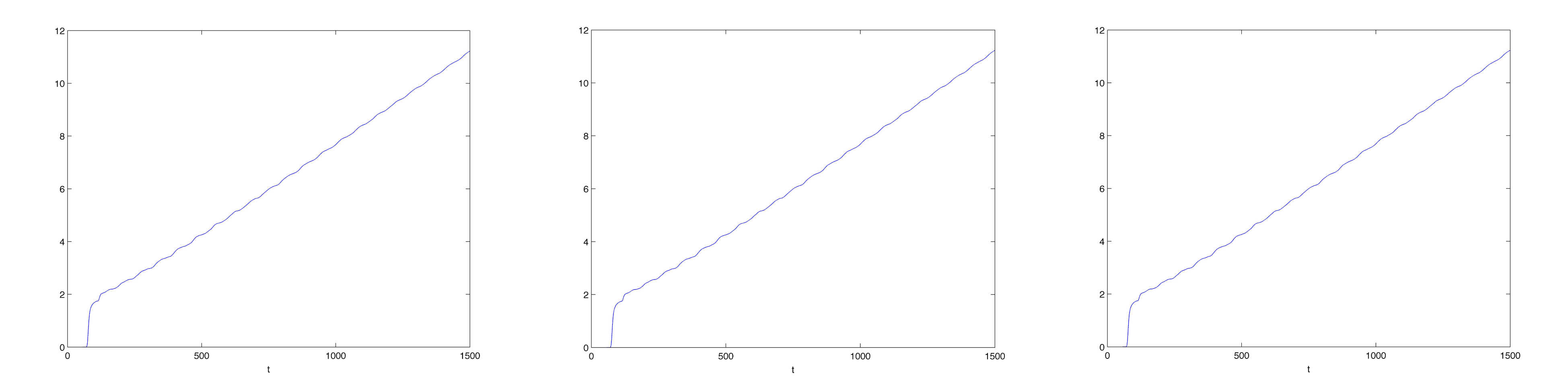
Figure 38: Evolution of the energy gain, $16000$ points, then $32000$ and $64000$.

We see from Figure 36 that the discrete energy indeed appears to diverge exponentially, but the divergence decreases like $h$ when we refine the discretisation. It seems to require a rather extreme precision to obtain a satisfactorily conserved quantity. However, the amplitude of the field and the energy gain (which relies on the calculation of the total energy only at $t=0$ and on the outgoing energy flux) do stabilise with very good accuracy when $h$ is refined (see Figures 37 and 38), which indicates that our observations in this article are reliable.

6 Conclusion

Usually, black hole bombs refer to setting a mirror around the ergoregion. Fields inside the mirror are thus forbidden to escape to infinity, creating linear instabilities thanks to repeated superradiant scattering in the ergoregion. This is the construction introduced by W. H. Press and S. A. Teukolsky for rotating black holes. In this article we have introduced a new type of black hole bomb. Namely, the mirror is inside the ergoregion but now the fields are located outside. Due to the presence of the mirror, the fields cannot fall into the black hole and can propagate to infinity. Because the field can still reach the ergoregion, this system also leads to linear instability. To our knowledge, this is the first time that this behaviour is exhibited. In addition, we have also introduced the so-called sandwich bomb: two mirrors form a cavity where the field is trapped and which contains part of the ergoregion. For these three types of black hole bombs, we have provided explicit numerical examples of linear instabilities, using a robust numerical method that ensures the conservation of a discrete energy consistent with the continuous one. The numerical study focuses on the cases of Reissner-Nordstr m and de Sitter-Reissner-Nordstr m backgrounds. The mirrors are either described by Neumann boundary conditions or by Dirichlet boundary conditions. In the case of Dirichlet conditions, apart from a single test where both boundary conditions give almost indistinguishable outputs, the instability seems to be less strong than when using Neumann boundary conditions. However, the qualitative behaviour is the same.

References

- [1] A. Bachelot, Superradiance and scattering of the charged Klein-Gordon field by a steplike electrostatic potential, J. Math. Pures Appl. 83 (2004), 1179–1239.
- [2] N. Besset, Decay of the local energy for the charged Klein-Gordon equation in the exterior de Sitter-Reissner-Nordstr m spacetime, arXiv:1812.09390, 2018.
- [3] J. Borthwick, Maximal Kerr de Sitter spacetimes, Class. Quant. Grav. 35 (2018) no.21, 215006, arXiv:1805.00243.
- [4] R. Brito, V. Cardoso, P. Pani, Superradiance, Lecture Notes in Physics 906 (Springer-Verlag, 2015), 221 pp.
- [5] S. Chandrasekhar, The mathematical theory of black holes, Oxford University Press, 1983.
- [6] P.M. Chesler, D.A. Lowe, Nonlinear evolution of the AdS4 black hole bomb, arXiv:1801.09711.
- [7] M. Dafermos, I. Rodnianski, Y. Shlapentokh-Rothman, A scattering theory for the wave equation on Kerr black hole exteriors, Ann. Scient. Éc. Norm. Sup. 4e série, t. 51, 2018, p. 371 à 486, arXiv:1412.8379.
- [8] J. C. Degollado and C. A. R. Herdeiro, Time evolution of superradiant instabilities for charged black holes in a cavity, Phys. Rev. D 89 (2014), 063005, arXiv:1312.4579.
- [9] O.J.C. Dias and R. Masachs, Charged black hole bombs in a Minkowski cavity, Class. Quant. Grav. 35 (2018) no.18, 184001, arXiv:1801.10176.
- [10] L. Di Menza and J.-P. Nicolas, Superradiance on the Reissner-Nordstr m metric, Class. Quant. Grav. 32 (2015), 145013–145040, arXiv:1411.3988.
- [11] G. Eskin, Superradiance initiated inside the ergoregion, Rev. Math. Phys. 28 (2016) no.10, 1650025, arXiv:1509.03197.
- [12] V. Georgescu, C. G rard, D. H fner, Asymptotic completeness for superradiant Klein-Gordon equations and applications to the de Sitter-Kerr metric, J. Eur. Math. Soc. (JEMS) 19 (2017), 8, 2371–2444, arXiv:1405.5304.
- [13] S. Green, S. Hollands, A. Ishibashi, R. Wald, Superradiant instabilities of asymptotically anti-de Sitter black holes, Classical Quantum Gravity 33 (2016),12, 125022, 22 pp, arXiv:1512.02644.
- [14] C. A. R. Herdeiro, J. C. Degollado and H. F. Rúnarsson, Rapid growth of superradiant instabilities for charged black holes in a cavity, Phys. Rev. D 88 (2013), 063003, arXiv:1305.5513.
- [15] P. Hintz, A. Vasy, The global nonlinear stability of the Kerr-de Sitter family of black holes, arXiv:1606.04014, 2016.
- [16] P. Hintz, Non-linear stability of the Kerr-Newman-de Sitter family of charged black holes, Ann. PDE 4 (2018), 1, Art. 11, 131 pp, arXiv:1612.04489.
- [17] S. Hod, Analytic treatment of the charged black-hole-mirror bomb in the highly explosive regime, Phys. Rev. D 88 (2013), 064055, arXiv:1310.6101.
- [18] S. Hod, The charged black-hole bomb: A lower bound on the charge-to-mass ratio of the explosive scalar field, Phys. Lett. B 755 (2016), 177–182, arXiv:1606.00444.
- [19] C.W. Misner, Interpretation of gravitational-wave observations, Phys. Rev. Lett. 28 (1972), 994–997.
- [20] M. Mokdad, Reissner-Nordstr m-de Sitter manifold: photon sphere and maximal analytic extension, Class. Quantum Grav. 34 (2017), 17, 175014, arXiv:1701.06982.
- [21] R. Penrose, Gravitational Collapse: The Role of General Relativity, Rivista del Nuovo Cimento, Numero Speziale 1 (1969), 252–276, re-printed in General Relativity and Gravitation, 34 (2002), 7, 1141–1165.
- [22] W. H. Press and S. A. Teukolsky, Floating Orbits, Superradiant Scattering and the Black-hole Bomb, Nature 238 (1972), 211–212.
- [23] J. M. Bardeen, W. H. Press and S. A. Teukolsky, Rotating black holes: Locally nonrotating frames, energy extraction, and scalar synchrotron radiation, Astrophys. J. 178 (1972) 347.
- [24] M. Richartz, A. Saa, Challenging the weak cosmic censorship conjecture with charged quantum particles, Phys. Rev. D 84, 104021 (2011), arXiv:1109.3364.
- [25] H. Witek, V. Cardoso, C. Herdeiro, A. Nerozzi, U. Sperhake, M. Zilh o, Black holes in a box: towards the numerical evolution of black holes in AdS spacetime, Phys. Rev. D 82 (2010) 104037, arXiv:1004.4633.
- [26] Y.B. Zel’dovich, Pis’ma Zh. Eksp. Teor. Fiz. 14 (1971), 270 [JETP Lett. 14 (1971), 180].
- [27] Y.B. Zel’dovich, Zh. Eksp. Teor. Fiz 62 (1972), 2076 [Sov. Phys. JETP 35 (1972), 1085].