ViTOR: Learning to Rank Webpages Based on Visual Features

Abstract.

The visual appearance of a webpage carries valuable information about the page’s quality and can be used to improve the performance of learning to rank (LTR). We introduce the Visual learning TO Rank (ViTOR) model that integrates state-of-the-art visual features extraction methods: (i) transfer learning from a pre-trained image classification model, and (ii) synthetic saliency heat maps generated from webpage snapshots. Since there is currently no public dataset for the task of LTR with visual features, we also introduce and release the ViTOR dataset, containing visually rich and diverse webpages. The ViTOR dataset consists of visual snapshots, non-visual features and relevance judgments for ClueWeb12 webpages and TREC Web Track queries. We experiment with the proposed ViTOR model on the ViTOR dataset and show that it significantly improves the performance of LTR with visual features.

1. Introduction

The design and appearance of a webpage are determining factors for a user to examine the page or to divert to another page (Nielsen, 1999, 2006; Pernice, 2017; Wang et al., 2014). However, relatively little is known about the potential of visual appearance to help determine the perceived relevance of a webpage. Recently, visual features, extracted from snapshots of webpages and search engine results pages, have been introduced into learning to rank (LTR) and have been shown to significantly improve the LTR performance (Fan et al., 2017; Zhang et al., 2018).

In this paper we continue studying LTR with visual features and propose the Visual learning TO Rank (ViTOR) model that integrates state-of-the-art visual features extraction methods. We present two implementations of the ViTOR model. First, we extract visual features from webpage snapshots using transfer learning and, in particular, by adopting the VGG-16 (Simonyan and Zisserman, 2014) and ResNet-152 (He et al., 2016) models pre-trained on ImageNet. Second, we introduce a novel set of visual features extracted from synthetic saliency heatmaps, which explicitly model how users view webpages (Shan et al., 2017).

Currently, there is no dataset available to support research on LTR with visual features. Fan et al. (2017) experimented with webpages from the GOV2 collection. However, GOV2 solely contains webpages within the .gov domain, i.e., pages with a relatively narrow scope, and, more importantly, these webpages do not contain their original images and styles. Hence, the GOV2 collection cannot fully support research on LTR with visual features, as it does not reflect visually rich and diverse webpages found on the internet today.

To overcome this issue, we release the ViTOR dataset that contains webpages from the ClueWeb12 collection and queries from the TREC Web Tracks 2013 & 2014 (Collins-Thompson et al., 2013, 2015). For each webpage of ClueWeb12 that also appears in the web tracks, the ViTOR dataset contains a snapshot and a set of content features, such as BM25 and PageRank. The introduced dataset is made publicly available.

To assess the performance of the proposed ViTOR model, we run experiments on the introduced ViTOR dataset. Our experiments confirm that visual features significantly improve the LTR performance, which is inline with previous findings (Fan et al., 2017). We also show that both implementations of the ViTOR model, namely transfer learning (with VGG-16 and ResNet-152) and synthetic saliency heatmaps, significantly outperform other LTR methods with visual features.

In summary, the main contributions of this work are: (i) We introduce transfer learning to extract visual features for LTR. (ii) We introduce synthetic saliency heatmaps as a novel set of LTR features. (iii) We introduce and publish ViTOR, an out-of-the-box dataset for LTR with visual features.

2. Related work

In this section, we discuss related research on the usage of visual information in LTR and the relation between visual appearance and user perception of webpages.

Using eye-tracking, Nielsen (2006) and Pernice (2017) demonstrate that webpage design and content placement influences the ability of users to find information they are looking for. Both studies show that by organizing the content in certain shapes (e.g., an F-shape), information can be navigated more efficiently. Wang et al. (2014) show that the size of the fixation areas measured using eye-tracking is larger on webpages with more content, which increases the likelihood that the attention of a user is distracted. Such studies highlight the importance of the visual appearance of a webpage and its effect on how users perceive pages, demonstrating that visual information has to be taken into account when ranking webpages.

Zhang et al. (2018) consider using visual features for LTR and, specifically, for learning to re-rank. The authors propose a multimodal architecture for re-ranking snippets on a SERP by learning their visual patterns. This work demonstrates that combining both visual and non-visual features can improve re-ranking performance.

The closest work to ours is the study by Fan et al. (2017), which uses visual information to rank webpages instead of re-ranking snippets within an existing ranking. The authors use snapshots of webpages to extract visual features for LTR and show that such visual features significantly improve retrieval performance. They feed snapshots through a neural network that attempts to model the previously mentioned F-shape. The output of this neural network is then concatenated with more traditional ranking signals, such as BM25 and PageRank. Finally, the proposed model (called ViP) is trained end-to-end using a pairwise loss. In our paper, we continue this line of research and propose the ViTOR model for LTR with visual features that makes use of the state-of-the-art visual feature extraction techniques and shows superior performance compared to ViP. Also, we develop and publish the ViTOR dataset that contains visually diverse webpages compared to the GOV2 dataset used in (Fan et al., 2017), which lacks visual diversity and, importantly, does not contain images and style information together with webpages.

3. ViTOR Model

In this section, we introduce the ViTOR model for LTR with visual features. The proposed model consists of three parts. First, we introduce the model architecture in Section 3.1. Then, in Section 3.2 we describe two visual feature extractors used by ViTOR: VGG-16 (Simonyan and Zisserman, 2014) and ResNet-152 (He et al., 2016), both pre-trained on ImageNet. Finally, in Section 3.3 we propose to enhance ViTOR by generating synthetic saliency heatmaps for each of the input images. The implementation of the proposed ViTOR model is available online.

3.1. Architecture

The ViTOR architecture is visualized in Figure 1. The process starts by taking an image $x_{i}$ (1) as an input to the visual feature extraction layer (2) in order to create a generic visual feature vector $x_{vf}$. These features are considered generic because they can be extracted using convolutional filters trained on a different dataset and task. In order to transform generic visual features into LTR specific visual features, we use $x_{vf}$ as an input to the visual feature transformation layer (3). This visual feature transformation layer outputs a visual feature vector $x_{vl}$ that can be used in combination with other LTR features.

Separating the visual feature extraction and transformation layers allows us to significantly reduce the computational requirements when using a pre-trained model for visual feature extraction. In Section 7.1 we further elaborate on how the computational requirements can be reduced. In Section 3.2 below, we demonstrate how transfer learning can be applied to use pre-trained visual feature extraction methods in combination with the ViTOR architecture.

The ViTOR architecture also makes use of content features $x_{c}$ (4), e.g., BM25, PageRank, etc. The final feature vector $x_{l}$ is constructed by concatenating the visual features $x_{vl}$ with the content features $x_{c}$. This final feature vector is then used as an input to the scoring component (5), which transforms the features into a single score $x_{s}$ for each query-document pair. The resulting model is trained end-to-end using a pairwise hinge loss with $L_{2}$ regularization similarly to (Fan et al., 2017). The scoring component uses a single fully connected layer with a hidden size of $10$ and dropout set to $10\%$, which showed good performance in preliminary experiments.

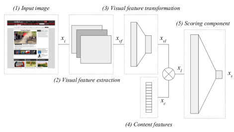
Figure 1. ViTOR architecture.

3.2. Visual feature extractors

In order to use webpage snapshots in LTR, the snapshots have to be converted to a vector representation that can then be used in combination with existing content features. Since preparing training data for LTR is costly and its amount is usually low, it is beneficial to use a visual feature extraction method that is already pre-trained. In this work we use the VGG-16 (Simonyan and Zisserman, 2014) and ResNet-152 (He et al., 2016) models, two well-explored image classification models which both have an implementation with ImageNet pre-trained parameters. Below, we describe how these two models are implemented within the ViTOR architecture.

VGG-16 (Simonyan and Zisserman, 2014) is commonly used for training transfer-learned models, because it provides a reasonable trade-off between effectiveness and simplicity (Shan et al., 2017). Its architecture consists of a set of convolutional layers and fully connected layers. The convolutional layers extract features from an input image, which are then used by the fully connected layers to classify the image. The convolutional layers of VGG-16 are generic with respect to an input and task (Donahue et al., 2014) and, thus, can be used as a visual feature extractor within the ViTOR architecture to create generic visual features $x_{vf}$. Hence, we use the convolutional layers as is, by freezing all the parameters during training. Because we do not alter any of the convolutional layers, the size of $x_{vf}$ is determined by the output of the convolutional layers in the original VGG-16 model, being $1\times 25088$.

The fully connected layers of VGG-16, instead, can be altered and retrained in order to be used with new inputs and tasks. Due to this, we utilize them as a visual feature transformation layer within the ViTOR architecture to produce LTR specific features $x_{vl}$. In particular, we replace the last fully connected layer of VGG-16 by a newly initialized fully connected layer. Then we optimize the parameters of all fully connected layers of VGG-16 during training. The size of $x_{vl}$ is set to $30$, as this size showed good performance in preliminary experiments.

The ResNet-152 (He et al., 2016) architecture was shown to outperform VGG-16 in ImageNet classification. The residual connections between convolutional layers of ResNet-152 allow for deeper networks to be trained without suffering from vanishing gradients. Similarly to VGG-16, ResNet-152 has convolutional layers that extract features from an input image, which are in turn used by a fully connected layer to classify each image. We use these convolutional layers as the visual feature extraction layer, which transforms $x_{i}$ to $x_{vf}$. All parameters of these convolutional layers are frozen during training. As with VGG-16, the size of $x_{vf}$ is determined by the output size of the original convolutional layers in the ResNet-152 model, $1\times 2048$.

Additionally, the original ResNet-152 architecture only has a single fully connected layer, which empirically showed to not be enough to successfully train the ViTOR model. Instead, we transform $x_{vf}$ to $x_{vl}$ by training a fully connected network from scratch. The transformation layer is constructed using three layers with each having $4096$ hidden units and a final layer resulting in $x_{vl}$ with a size of $30$, which was empirically found to provide good performance in preliminary experiments.

3.3. Saliency heatmaps

In order to increase the ability to learn the visual quality of a webpage, we propose to explicitly model the user viewing pattern through synthetic saliency heatmaps. The use of saliency heatmaps could be advantageous compared to the use of raw snapshots for the following reasons. First, synthetic saliency heatmaps explicitly learn to predict how users perceive webpages by training an end-to-end model on actual eye-tracking data. We expect this information to better correlate with webpage relevance compared to raw snapshots. Second, saliency heatmaps reduce the average storage requirements by up to 90%, because they are gray-scale images and have large areas of the same color, which can be stored efficiently. This makes the use of saliency heatmaps attractive for practical applications. Figure 2 shows example snapshots with their corresponding heatmaps (first and third columns respectively).

Following (Shan et al., 2017), we use a two-stage transfer learning model that learns how to predict saliency heatmaps on webpages. Similarly to the visual feature extraction approaches above, (Shan et al., 2017) takes a pre-trained image recognition model and finetunes the output layers on the following two datasets in order respectively: (i) SALICON (Jiang et al., 2015), a large dataset containing saliency heatmaps created with eye-tracking hardware on natural images, and (ii) the webpage saliency dataset from (Shen and Zhao, 2014), a smaller dataset containing saliency heatmaps created with eye-tracking hardware on webpages.

The trained model is used to convert a raw snapshot into a synthetic saliency heatmap. This heatmap is then used as an input image $x_{i}$ for the ViTOR model (see Figure 1).

(a)

(b)

(c)

(d)

(e)

(f)

(g)

(h)

(i)

Figure 2. Examples of a vanilla snapshot, a red highlighted snapshot, and a saliency heatmap from left to right, respectively.

4. ViTOR Dataset

In this section, we introduce the ViTOR dataset for LTR with visual features. Section 4.1 contains information about the underlying ClueWeb12 collection and TREC Web Track topics. Section 4.2 explains how the snapshots for ClueWeb12 are acquired. Section 4.3 discusses content features, such as BM25 and TF-IDF, included in the ViTOR dataset. Finally, Section 4.4 gives an overview of the structure in which the ViTOR dataset is presented and published.

4.1. ClueWeb12 & TREC Web Track

For the ViTOR dataset we choose to use a combination of the ClueWeb12 document collection and the topics from the TREC Web Tracks 2013 & 2014 (Collins-Thompson et al., 2013, 2015), because this is currently the most recent combination of a large-scale webpage collection together with judged queries (with graded relevance).

ClueWeb12 is a highly diverse collection of webpages scraped in the first half of 2012. The total collection contains over 700 million webpages. We only use ClueWeb12 webpages that have judgements for any of the 100 queries in the TREC Web Tracks 2013 & 2014. In total, there are 28,906 judged webpages. Table 1 shows the breakdown of the total number of webpages and different relevance labels in the combined set of topics from 2013 and 2014.

Table 1. Number of webpages per source and the corresponding breakdown of TREC Web Track relevance grades.

Count/Label	TREC Web	Wayback	ClueWeb12	No image
Total	28,906	23,249	5,392	265
Nav grade (4)	40	36	4	0
Key grade (3)	409	347	62	0
Hrel grade (2)	2,534	2,222	295	17
Rel grade (1)	6,832	5,679	1,123	30
Non grade (0)	18,301	14,395	3,701	205
Junk grade (-2)	790	570	207	13

4.2. Snapshots

Although each entry in the ClueWeb12 collection contains the webpage’s HTML source, many pages lack styling and images files in order to render the full page. To overcome this issue, we use the Wayback Machine, which offers various archived versions of webpages with styling and images since 2005. For each page in ClueWeb12, that is also judged in the TREC Web Tracks 2013 & 2014, we scrape an entry on the Wayback Machine that is closest to the original page scrape date as recorded in ClueWeb12. A snapshot is then taken using a headless instance of the Firefox browser. To reproduce (Fan et al., 2017), we also create a separate query-dependent dataset with the same snapshots where all query words are highlighted in red (HEX value: #ff0000). Examples of snapshots and snapshots with highlights are shown in Figure 2 (first two columns).

Since the Wayback Machine does not contain an archived or working version of each webpage in the ClueWeb12 collection, a filtering process is introduced to maximize the quality of each snapshot. Using the following criteria, a snapshot is selected for each available webpage: (1) Each webpage is requested from the Wayback Machine. (2) A webpage that is not on the Wayback Machine, times out, throws a JavaScript error, or results in a PNG snapshot smaller than 100KB is marked as broken. Such webpages are rendered again using the online rendering service provided by ClueWeb12. (3) A manual selection is made between all webpages that are rendered from both sources. The Wayback version is used if it contains more styling elements and if the content is the same as in the rendering service. Otherwise, the rendering service version is used.

As a result, most of the 28,906 judged webpages have a corresponding snapshot from either the Wayback Machine or ClueWeb12 rendering service. Only 265 documents did not pass the filtering and were discarded. Table 1, row one, summarizes the results of the ViTOR dataset acquisition process. The table also shows the distribution of judgment scores among the snapshots that were taken from the Wayback Machine and ClueWeb12 rendering service.

4.3. Non-visual features

In LTR, documents are ranked based on various types of features, such as content features (e.g., BM25), quality indicators (e.g., PageRank) and behavioral features (e.g., CTR). In order to use the ViTOR dataset to measure the effect of visual features, we also add a set of content features and quality indicators, listed in Table 2. These 11 features are chosen so that they resemble most informative features of the most recent LETOR 4.0 dataset (Qin and Liu, 2013) and are easy to compute (see Section 7.2 for a detailed comparison of different feature sets). Also note that behavioral features, such as CTR, are not available for the TREC Web Tracks.

The content features, such as TF-IDF and BM25, are computed by doing a full pass over the complete ClueWeb12 collection. The PageRank scores are taken from the ClueWeb12 Related Data section. The following modifications based on the feature transformations described in LETOR are made to stabilize training: (1) Free parameters $k_{1}$, $k_{3}$ and $b$ for BM25 were set to $2.5$, $0$ and $0.8$, respectively. (2) Since the PageRank scores are usually an order of magnitude smaller than all other scores, we multiply them by $10^{5}$. (3) The log transformation is applied to each feature. (4) The log-transformed features are normalized per query.

Table 2. Non-visual features provided with the ViTOR dataset.

Id	Description	Id	Description	Id	Description
1	Pagerank	5	Content TF-IDF	9	Title IDF
2	Content length	6	Content BM25	10	Title TF-IDF
3	Content TF	7	Title length	11	Title BM25
4	Content IDF	8	Title TF

4.4. Final collection

In summary, the ViTOR dataset contains: (i) a directory with webpage snapshots (Section 4.2), and (ii) a set of files with content features divided into folds (Section 4.3). Each snapshot is stored as a PNG file that can be identified by its corresponding ClueWeb12 document id. The non-visual features are stored in LETOR formatted files containing the raw, logged and query normalized values. The query normalized values are randomly split per query into five equal partitions. These partitions are then used to create five folds, where each fold contains three partitions for training and the remaining two partitions for validation and testing.

5. Experimental Setup

In this section, we discuss the configurations of the ViTOR architecture, baselines and metrics used during our experiments.

ViTOR configurations.. We experiment with four configurations of the ViTOR architecture. ViTOR baseline refers to the ViTOR model with only content features. This configuration is trained by feeding content features into the scoring component directly, without adding any visual features. ViTOR snapshots and ViTOR highlights use visual features extracted from vanilla snapshots of webpages and from snapshots of webpages with highlighted query terms, respectively. Finally, ViTOR saliency uses visual features extracted from synthetic saliency heatmaps. The snapshots, highlights and saliency heatmaps for each model respectively are used as the input image (component (1) of Figure 1. For the ViTOR configurations with visual features, we experiment with both VGG-16 and ResNet-152 visual feature extraction methods. The learning rates for VGG-16 and ResNet-152 are set to and $0.0001$ and $0.00005$, respectively. Each experimental run is generated using the Adam optimizer (Kingma and Ba, 2014) with a batch size of $100$.

Baselines. We compare our proposed ViTOR model to the ViP model by Fan et al. (2017), the only existing LTR method that uses visual features. We train ViP on both vanilla and highlighted snapshots with the resulting configurations being ViP snapshots and ViP highlights, respectively. Following (Fan et al., 2017), we also compare the ViTOR model to a number of content-based ranking methods, namely BM25 and state-of-the-art LTR techniques, such as RankBoost, AdaRank, and LambdaMart.

Metrics. To measure the retrieval performance, we use precision and ndcg at $\{1,10\}$ and MAP. Statistical significance is determined using a two-tailed paired t-test (p-value $\leq 0.05$).

6. Results

In this section, we present experiments that are set out to test the following: (1) the ViTOR model improves the LTR performance when introducing visual features, (2) synthetic saliency heatmaps improve the LTR performance when used as an input the ViTOR model, and (3) the ViTOR model improves both visual and non-visual state-of-the-art ranking methods.

6.1. ViTOR model with VGG-16 and ResNet-152

In Table 3, we compare the performance of the ViTOR model when used with and without visual features. The first row shows the ViTOR baseline, when using only the content features as an input to the scoring component. The second to fifth rows show the performance of using VGG-16 and ResNet-152 with both vanilla and highlighted snapshots. These results clearly show that both VGG-16 and ResNet-152 visual feature extraction methods significantly improve the performance compared to the ViTOR baseline.

When comparing the results of the ViTOR model with visual features, we observe the following: (i) The highest ranking performance is achieved by using VGG-16 on the highlighted snapshots. (ii) For VGG-16, the values of all metrics are consistently better for highlighted snapshots compared to vanilla snapshots, which is in line with the findings of (Fan et al., 2017) and is to be expected: highlighted snapshots carry more information compared to vanilla snapshots. Based on these results, we conclude that the use of visual features in LTR significantly improves performance and that highlighted snapshots should on average be preferred over vanilla snapshots.

Table 3. Results for the ViTOR model using only content features (baseline), vanilla snapshots, highlighted snapshots, and saliency heatmaps. All results significantly improve over the ViTOR baseline. Best results are shown in bold.

	p@1	p@10	ndcg@1	ndcg@10	MAP
ViTOR baseline	0.338	0.370	0.189	0.233	0.415
VGG snapshots	0.514	0.484	0.292	0.324	0.442
ResNet snapshots	0.550	0.452	0.310	0.301	0.437
VGG highlights	0.560	0.520	0.323	0.346	0.456
ResNet highlights	0.530	0.463	0.305	0.312	0.440
VGG saliency	0.554	0.453	0.310	0.302	0.422
ResNet saliency	0.560	0.476	0.333	0.321	0.442

6.2. ViTOR model with saliency heat maps

The last two rows of Table 3 show the performance of the ViTOR model when using synthetic saliency heat maps as an input. The visual features are learned using both VGG-16 and ResNet-152. In this case, ResNet-152 consistently outperforms VGG-16. Although the highlighted snapshots with VGG-16 still outperform ResNet-152 with saliency heat maps on p@10, ndcg@10 and MAP, the saliency heat maps with ResNet-152 match and outperform VGG-16 with highlighted snapshots when looking at p@1 and ndcg@1. Hence, saliency heat maps should be preferred in applications where early precision is important, while highlighted snapshots should be used when a high overall performance is needed.

6.3. Baseline comparison

Table 4 compares the performance of the ViTOR model to BM25, non-visual LTR methods and the ViP model by Fan et al. (2017). Specifically, the table shows the performance of VGG-16 with highlighted snapshots and of ResNet-152 with synthetic saliency heatmaps, as these are the best-performing variants of the ViTOR model according to Table 3. Both methods have a significant performance increase compared to BM25, almost doubling the metrics values in many cases.

When comparing to non-visual LTR methods, both ViTOR implementations show consistently better performance. However, not all metrics are improved significantly. We attribute this to the fact that, similarly to (Fan et al., 2017), the LTR component of the ViTOR model is based on pairwise hinge loss, which is a relatively simple loss function.

Finally, we compare the ViTOR implementations to ViP, the only existing LTR method with visual features. Here, we clearly see that both our implementations significantly outperform ViP on all metrics. Also note, that ViP loses to two out of three non-visual LTR baselines, namely RankBoost and LambdaMart. We believe this is due to the reason discussed above: ViP uses pairwise hinge loss as the LTR component (Fan et al., 2017), which may be suboptimal.

The above results show that the proposed ViTOR model outperforms baselines, whether they are supervised or unsupervised, use visual features or not. However, to achieve consistent significant improvements compared to the state-of-the-art LTR methods, different loss functions within the ViTOR model have to be investigated.

Table 4. Results for the VGG-16 with highlighted snapshots, ResNet-152 with saliency heatmaps, and baselines. $\dagger$ indicates a significant decrease in performance compared to VGG highlights and $\ddagger$ indicates a significant decrease in performance compared to both ViTOR implementations. Best results are shown in bold.

	p@1	p@10	ndcg@1	ndcg@10	MAP
BM25	0.300‡	0.316‡	0.153‡	0.188‡	0.350‡
RankBoost	0.450	0.444	0.258	0.288†	0.427
AdaRank	0.290‡	0.357‡	0.149‡	0.227‡	0.398
LambdaMart	0.470	0.420†	0.256	0.275†	0.418
ViP snapshots	0.392‡	0.398‡	0.217‡	0.254‡	0.421‡
ViP highlights	0.418‡	0.416‡	0.239‡	0.269‡	0.422‡
VGG highlights	0.560	0.520	0.323	0.346	0.456
ResNet saliency	0.560	0.476	0.333	0.321	0.442

7. Discussion

In this section, we address two practical aspects of the proposed ViTOR model and dataset: (i) the number of parameters of the ViTOR model and corresponding optimizations, and (ii) the performance of content features included in the ViTOR dataset.

7.1. Training and inference optimization

Both training and inference using deep convolutional networks are generally computationally expensive. By separating the feature extraction and transformation layers in the proposed ViTOR architecture (see Figure 1) we allow powerful computational optimizations for both training and inference.

Training optimization. Although we freeze the parameters in the visual feature extraction layer (component (2) of Figure 1) when using a pre-trained model, we still need to compute the output from all the frozen parameters during the forward propagation. We can avoid the computational cost associated with the forward propagation on the frozen layers by storing the output of the visual feature extraction layer to disk prior to training. By storing these vectors to disk, we leave only the parameters of the fully connected layers (component (3) of Figure 1) to be calculated and stored in memory during the forward propagation.

By applying the above procedure, we can reduce the number of parameters of the ViTOR model. When using VGG-16, the visual feature extraction layer consists of $14,714,688$ parameters, which is $12.3\%$ of the parameters in the ViTOR model. When using ResNet-152, the visual feature extraction layer consists of $58,144,239$ parameters, which is $49.5\%$ of the parameters in the ViTOR model.

By using the stored output of the visual feature extraction layer $x_{vf}$ instead of an actual image $x_{i}$ as the input of the ViTOR model, we reduce the size of each input by $84.7\%$ and $98.6\%$ for VGG-16 and ResNet-152 respectively. This reduction in input size further reduces the memory required for training the model.

Real-time inference optimization. When using LTR in a large-scale production environment, the impact of newly introduced LTR features (visual features, in our case) on real-time computational requirements is of major concern.

Since both the vanilla snapshots and synthetic saliency heatmaps are query independent, the output of the visual feature transformation layer (component (3) of Figure 1) does not change for different document/query pairs. This enables offline inference, leaving only the scoring component to be inferred in real-time. Since a visual feature vector is has $1\times 30$, using the offline inferred feature vector would result in a LTR model with $30+11=41$ features. This increase in parameters is negligible in terms of computational costs.

7.2. Benchmarking content features

In LTR research, both the amount and type of considered features vary widely per dataset and study. The most recent LETOR 4.0 dataset (Qin and Liu, 2013) contains 46 features extracted for webpages from the GOV2 dataset and queries from the million query tracks 2007 and 2008 (MQ2007 and MQ2008). In the ViTOR dataset, we use 11 features that are a subset of the 46 features of LETOR (see Table 2). These 11 features are chosen to be both informative and easy to compute. Here, we compare our subset of 11 features to the full set of 46 features. The experiments are run on the GOV2 dataset and MQ2007 queries. The LTR methods considered are the same as in Section 6, namely RankBoost, AdaRank, and LambdaMart.

The results of running the considered LTR methods using both 46 and 11 features are shown in Table 5. From these results, we see that the number of features has a significant effect on the performance of AdaRank. However, for the best-performing RankBoost and LambdaRank methods the drop in performance is minor when using 11 features instead of 46 features. This indicates that the chosen 11 features included in the ViTOR dataset form a reasonable trade-off between effectiveness and computation cost.

Table 5. Comparison of 46 LETOR features and 11 LETOR features that are also used in ViTOR.

	p@1	p@10	ndcg@1	ndcg@10	MAP
RankBoost - 46	0.453	0.371	0.391	0.430	0.457
RankBoost - 11	0.448	0.372	0.381	0.431	0.453
AdaRank - 46	0.420	0.360	0.367	0.424	0.449
AdaRank - 11	0.385	0.287	0.364	0.394	0.386
LambdaMart - 46	0.452	0.384	0.405	0.444	0.463
LambdaMart - 11	0.448	0.380	0.397	0.443	0.455

8. Conclusion

In this paper, we considered the problem of LTR with visual features. We proposed the ViTOR model that extracts visual features from webpage snapshots using transfer learning (specifically, pre-trained VGG-16 and ResNet-152 models) and synthetic saliency heatmaps. In both cases the extracted visual features significantly improved the LTR performance. We also showed that the proposed ViTOR model significantly outperformed the visual LTR baselines.

In addition to the model, we released the ViTOR dataset, containing visually rich and diverse webpages with corresponding snapshots. With the ViTOR dataset it is now possible to comprehensively study LTR with visual features.

One direction for future work is the study of state-of-the-art LTR methods, such as RankBoost and LambdaMart, within the scoring components of the ViTOR model. This could improve performance without changing the visual feature extraction and transformation components. Another promising direction is to combine multiple visual features, i.e., visual features extracted from vanilla snapshots, snapshots with highlights and saliency heatmaps. Other visual feature extractors, such as the CapsuleNet (Sabour et al., 2017) model, which is able to learn spatial relations in images, might also provide additional performance. Other methods of combining visual and textual features might also be worth exploring. Future work could also investigate the robustness of this method when using various rendering variations, e.g., different browser, resolutions. Finally, performing a more qualitative analysis on which elements cause improvements in LTR with visual features would be interesting, e.g., by interpreting the filters in the feature extractor (Olah et al., 2018).

Code and data

Both the ViTOR dataset and the code used to run the experiments in this paper are available online.

Acknowledgements

The Spark experiments in this work were carried out on the Dutch national e-infrastructure with the support of SURF Cooperative. Thanks to the Amsterdam Robotics Lab for using their computational resources. Thanks to Jamie Callan and his team for providing access to the online services for ClueWeb12.

This research was partially supported by Ahold Delhaize, the Association of Universities in the Netherlands (VSNU), and the Innovation Center for Artificial Intelligence (ICAI). All content represents the opinion of the authors, which is not necessarily shared or endorsed by their respective employers and/or sponsors.

References

- (1)
- Collins-Thompson et al. (2013) Kevyn Collins-Thompson, Paul Bennett, Fernando Diaz, Charlie Clarke, and Ellen M Voorhees. 2013. TREC 2013 Web Track overview. In TREC. NIST.
- Collins-Thompson et al. (2015) Kevyn Collins-Thompson, Craig Macdonald, Paul Bennett, Fernando Diaz, and Ellen M Voorhees. 2015. TREC 2014 Web Track overview. In TREC. NIST.
- Donahue et al. (2014) Jeff Donahue, Yangqing Jia, Oriol Vinyals, Judy Hoffman, Ning Zhang, Eric Tzeng, and Trevor Darrell. 2014. Decaf: A deep convolutional activation feature for generic visual recognition. In ICML. 647–655.
- Fan et al. (2017) Yixing Fan, Jiafeng Guo, Yanyan Lan, Jun Xu, Liang Pang, and Xueqi Cheng. 2017. Learning visual features from snapshots for web search. In CIKM. ACM, 247–256.
- He et al. (2016) Kaiming He, Xiangyu Zhang, Shaoqing Ren, and Jian Sun. 2016. Deep residual learning for image recognition. In CVPR. 770–778.
- Jiang et al. (2015) Ming Jiang, Shengsheng Huang, Juanyong Duan, and Qi Zhao. 2015. Salicon: Saliency in context. In CVPR. 1072–1080.
- Kingma and Ba (2014) Diederik P Kingma and Jimmy Ba. 2014. Adam: A method for stochastic optimization. arXiv preprint arXiv:1412.6980 (2014).
- Nielsen (1999) Jakob Nielsen. 1999. Designing web usability: The practice of simplicity. New Riders Publishing.
- Nielsen (2006) Jakob Nielsen. 2006. F-shaped pattern for reading web content. Jakob Nielsen’s Alertbox. (2006).
- Olah et al. (2018) Chris Olah, Arvind Satyanarayan, Ian Johnson, Shan Carter, Ludwig Schubert, Katherine Ye, and Alexander Mordvintsev. 2018. The Building Blocks of Interpretability. Distill (2018).
- Pernice (2017) Kara Pernice. 2017. F-shaped pattern of reading on the web: Misunderstood, but still relevant (Even on mobile). nngroup.com. (2017).
- Qin and Liu (2013) Tao Qin and Tie-Yan Liu. 2013. Introducing LETOR 4.0 Datasets. arXiv preprint arXiv:1306.2597 (2013).
- Sabour et al. (2017) Sara Sabour, Nicholas Frosst, and Geoffrey E Hinton. 2017. Dynamic routing between capsules. In NIPS. 3859–3869.
- Shan et al. (2017) Wei Shan, Guangling Sun, Xiaofei Zhou, and Zhi Liu. 2017. Two-stage transfer learning of end-to-end convolutional neural networks for webpage saliency prediction. In IScIDE. Springer, 316–324.
- Shen and Zhao (2014) Chengyao Shen and Qi Zhao. 2014. Webpage saliency. In ECCV. Springer, 33–46.
- Simonyan and Zisserman (2014) Karen Simonyan and Andrew Zisserman. 2014. Very deep convolutional networks for large-scale image recognition. arXiv preprint arXiv:1409.1556 (2014).
- Wang et al. (2014) Qiuzhen Wang, Sa Yang, Manlu Liu, Zike Cao, and Qingguo Ma. 2014. An eye-tracking study of website complexity from cognitive load perspective. Decision Support Systems 62 (2014), 1–10.
- Zhang et al. (2018) Junqi Zhang, Yiqun Liu, Shaoping Ma, and Qi Tian. 2018. Relevance Estimation with Multiple Information Sources on Search Engine Result Pages. In CIKM. ACM, 627–636.