Controlled Generation of Dark-Bright Soliton Complexes
in Two-Component and Spinor Bose-Einstein Condensates

Abstract

We report on the controlled creation of multiple soliton complexes of the dark-bright type in one-dimensional two-component, three-component and spinor Bose-Einstein condensates. The formation of solitonic entities of the dark-bright type is based on the so-called matter wave interference of spatially separated condensates. In all three cases a systematic numerical study is carried out upon considering different variations of each systems’ parameters both in the absence and in the presence of a harmonic trap. It is found that manipulating the initial separation or the chemical potential of the participating components allows us to tailor the number of nucleated dark-bright states. Particularly, the number of solitons generated increases upon increasing either the initial separation or the chemical potential of the participating components. Similarities and differences of the distinct models considered herein are showcased, while the robustness of the emerging states is illustrated via direct numerical integration demonstrating their long time propagation. Importantly, for the spinorial system, we unravel the existence of beating dark soliton arrays that are formed due to the spin-mixing dynamics. These states persist in the presence of a parabolic trap, often relevant for associated experimental realizations.

I Introduction

Among the nonlinear excitations that arise in Bose-Einstein condensates (BECs) Anderson et al. (1995); Davis et al. (1995), matter-wave dark Frantzeskakis (2010) and bright Abdullaev et al. (2005) solitons constitute the fundamental signatures. These structures stem from the balance between dispersion and nonlinearity and exist in single component BECs with repulsive and attractive interparticle interactions respectively Zakharov and Shabat (1972, 1973). Also more complex structures consisting of dark solitons in one component and bright solitons hosted in the second component of a binary BEC have been experimentally realized Becker et al. (2008); Middelkamp et al. (2011); Hamner et al. (2011); Yan et al. (2011); Hoefer et al. (2011); Yan et al. (2012). The existence and robustness of a single dark-bright (DB) soliton as well as interactions between multiple DB states both with each other as well as with impurities have been exhaustively studied in such settings Brazhnyi and Pérez-García (2011); Yin et al. (2011); Yan et al. (2011); Achilleos et al. (2011); Álvarez et al. (2013); Yan et al. (2015); Karamatskos et al. (2015); Katsimiga et al. (2017a, b, 2018a). In contrast to single component setups, DB solitons are the building blocks that emerge in repulsively interacting two-component BECs Kevrekidis and Frantzeskakis (2016). In such a repulsive environment (where bright solitonic states cannot exist on their own) DB states owe their existence to the effective potential created by each of the participating dark solitons into which each of the bright solitons is trapped and consequently waveguided Trillo et al. (1988); Christodoulides (1988); Ostrovskaya and Kivshar (1998). This waveguiding notion has been firstly introduced in the context of nonlinear optics Afanasyev et al. (1989); Kivshar and Turitsyn (1993); Christodoulides et al. (1996); Buryak et al. (1996); Sheppard and Kivshar (1997); Chen et al. (1997); Kivshar and Luther-Davies (1998); Ostrovskaya et al. (1999); Park and Shin (2000). Besides the aforementioned two-component BECs, the experimental realization of spinor BECs Stamper-Kurn and Ketterle (2001); Chang et al. (2004, 2005); Kawaguchi and Ueda (2012); Stamper-Kurn and Ueda (2013) offers new possibilities of investigating the different soliton entities that arise in them Ohmi and Machida (1998); Tsuchida and Wadati (1998); Ieda et al. (2004a, b); Ieda (2005); Li et al. (2005); Wadati and Tsuchida (2005); Ieda et al. (2006); Uchiyama et al. (2006); Ieda et al. (2007); Zhang et al. (2007); Kurosaki and Wadati (2007); Dabrowska-Wüster et al. (2007); Kawaguchi and Ueda (2012); Stamper-Kurn and Ueda (2013). In this context, more complex compounds in the form of dark-dark-bright (DDB) and dark-bright-bright (DBB) solitons have been theoretically predicted Nistazakis et al. (2008); Xiong and Gong (2010) and very recently experimentally observed Bersano et al. (2018).

There are multiple ways of generating single and multiple dark solitons Katsimiga et al. (2018b) (with the latter sometimes referred to as the dark soliton train Brazhnyi and Kamchatnov (2003)), in single component BECs. Common techniques consist of density engineering Dutton et al. (2001); Engels and Atherton (2007); Shomroni et al. (2009), phase engineering Burger et al. (1999); Denschlag et al. (2000); Anderson et al. (2001); Becker et al. (2008), and collision of two spatially separated condensates Weller et al. (2008); Hoefer et al. (2009) (see also Scherer et al. (2007a) for an interesting geometric higher dimensional implementation of the latter process so as to produce vortices). This latter generation process can be thought of as a consequence of matter wave interference of the two condensates Reinhardt and Clark (1997); Scott et al. (1998); Weller et al. (2008); Theocharis et al. (2010). Additionally, also known are the conditions under which the controllable formation of dark soliton trains can be achieved Reinhardt and Clark (1997); Scott et al. (1998); Brazhnyi and Kamchatnov (2003); Weller et al. (2008); Theocharis et al. (2010). In particular, it has been demonstrated that the number of generated dark solitons depends on the phase and momentum of the colliding condensates Weller et al. (2008); Theocharis et al. (2010). On the contrary, in multi-component settings such as two-component and spinor BECs the dynamics is much more involved. In this context, large scale counterflow experiments exist according to which also DB soliton trains can be created Hamner et al. (2011). However, to the best of our knowledge a systematic study regarding the controllable formation of these more complex solitonic structures and their relevant extensions in spinorial BECs is absent in the current literature. This controlled formation process represents the core of the present investigation.

Motivated by recent experimental advances in one-dimensional (1D) two-component Hamner et al. (2011); Middelkamp et al. (2011); Yan et al. (2011); Hoefer et al. (2011); Yan et al. (2012) and more importantly spinor BECs Bersano et al. (2018), here we report on the controllable generation of multiple soliton complexes. These include DB solitons in two-component BECs, and variants of these structures, i.e. DDB and DBB soliton arrays, in three-component and spinor BECs. For all models under consideration, the creation process of the relevant states is based on the so-called matter wave interference of separated condensates being generalized to multi-component systems. In all cases, the homogeneous setting is initially discussed and subsequently we generalize our findings to the case where an experimentally motivated parabolic confinement, i.e. trap, is present.

Specifically, for the homogeneous settings investigated herein the creation process is as follows. To set up the interference dynamics, an initial inverted rectangular pulse (IRP) is considered Zakharov and Shabat (1973) for the component(s) that will host later on the dark solitons. The counterflow process relies on the collision of the two sides of the pulse. For the remaining component(s), that will host later on the bright solitons, a Gaussian pulse initial condition is introduced. It is shown that such a process ensures the formation of dark soliton arrays the number of solitons in which can be manipulated by properly adjusting the width of the initial IRP. Additionally, the dispersive behavior of the Gaussian used, due to the defocusing nature of each system, allows its confinement in the effective potential created by each of the formed dark solitons and thus leads to the formation of the desired localized humps. The latter are trapped and subsequently waveguided by the corresponding dark solitons. In this way, arrays of robustly propagating DB, DDB and DBB solitons in two-component, three-component and spinor systems are showcased. Indeed, and as far as the two-component system is concerned, we verify among others, that during evolution the trajectory of each of the nucleated pairs follows the analytical predictions stemming from the exact single DB state. Also for the three-component scenario generalized expressions for the soliton characteristics are extracted and deviations from the latter when different initializations are considered are discussed in detail. In the spinor setting the controlled nucleation of arrays consisting of multiple DBB and DDB solitons is demonstrated, a result that can be tested in current state-of-the-art experiments Bersano et al. (2018). Remarkably enough, in the DDB nucleation process, the originally formed DDB arrays soon after their formation transition into beating dark solitons that gradually arise in all three hyperfine components Park and Shin (2000); Öhberg and Santos (2001); Hoefer et al. (2011); Yan et al. (2012). This transition stems, as we will explain in more detail below, from the spin-mixing dynamics that allows for particle exchange among the hyperfine components.

After the proof-of-principle in the spatially homogeneous case, we turn to the harmonically trapped models, where once again in order to induce the dynamics, counterflow techniques are utilized Weller et al. (2008); Theocharis et al. (2010); Hamner et al. (2011). Now the background on top of which the spatially separated BECs are initially set up asymptotes to a Thomas-Fermi (TF) profile for all the participating components. The counterflowing components are initially relaxed in a double-well potential, while the other component encounters a tight harmonic trap. The system is then released and evolves in a common parabolic potential. It is found that by properly adjusting the initial separation of the condensates or the chemical potential in each of the participating components leads to the controlled nucleation of a desired number of soliton structures, in this case too, with similar functional dependences of the soliton number on the system characteristics as above. For the two- and three-component systems it is found that the generated soliton arrays travel within the parabolic trap oscillating and interacting with one another for large evolution times. Finally, in the genuine spinor case and for a DDB formation process again arrays but of oscillating and interacting beating dark solitons emerge in all hyperfine components. We find that these states occur earlier in time when compared to the homogeneous scenario. The spin-mixing dynamics is explained via monitoring the population of the three hyperfine states. Damping oscillations of the latter are observed in line with the predictions in spinor $F=1$ BECs Pu et al. (1999); Chang et al. (2005).

The work-flow of this presentation proceeds as follows. In Sec. II we present the different models under consideration. In particular, the spinor $F=1$ BEC system is initially introduced and the complexity of the model is reduced all the way down to the single-component setting. Subsequently, a brief discussion summarizing prior results regarding the controllable generation of dark soliton trains emerging in single-component systems is provided. Finally here, we comment on the initial state preparation utilized herein in order to controllably generate multiple soliton complexes of the DB type in multi-component BECs. Sec. III contains our numerical findings ranging from two-component to spinor BEC systems. In all the cases presented, the homogeneous setting is initially investigated, and we next elaborate on the relevant findings in the presence of traps. To conclude this work, in Sec. IV we summarize our findings and we also discuss future directions.

II Models and setups

II.1 Equations of motion

We consider a 1D harmonically confined spinor $F=1$ BEC. Such a system can be described by three coupled Gross-Pitaevskii equations (CGPEs), one for each of the three hyperfine states $m_{F}=-1,0,+1$, of e.g. a ⁸⁷Rb gas. In the mean-field framework the wavefunctions, ${\bf\Psi}(x,t)=\left[\Psi_{+1}(x,t),\Psi_{0}(x,t),\Psi_{-1}(x,t)\right]^{T}$, of the aforementioned hyperfine components are known to obey the following GPEs (see e.g. Stamper-Kurn and Ueda (2013); Bersano et al. (2018)):

$$i\partial_{t}\Psi_{\pm 1} ={\cal{H}}_{0}\Psi_{\pm 1}+g_{n}\left(|\Psi_{+1}|^{2}+|\Psi_{0}|^{2}+|\Psi_{-1}|^{2}\right)\Psi_{\pm 1}$$

$$+g_{s}\left(|\Psi_{\pm 1}|^{2}+|\Psi_{0}|^{2}-|\Psi_{\mp 1}|^{2}\right)\Psi_{\pm 1}+g_{s}\Psi_{0}^{2}\Psi^{*}_{\mp 1},$$

$$i\partial_{t}\Psi_{0} ={\cal{H}}_{0}\Psi_{0}+g_{n}\left(|\Psi_{+1}|^{2}+|\Psi_{0}|^{2}+|\Psi_{-1}|^{2}\right)\Psi_{0}$$

$$+g_{s}\left(|\Psi_{+1}|^{2}+|\Psi_{-1}|^{2}\right)\Psi_{0}+2g_{s}\Psi_{+1}\Psi^{*}_{0}\Psi_{-1}.$$

In the above expressions the asterisk denotes the complex conjugate and ${\mathcal{H}}_{0}=-\frac{1}{2}\partial^{2}_{x}+V(x)$ is the single-particle Hamiltonian. Here, $V(x)=\left(1/2\right)\Omega^{2}x^{2}$ denotes (unless indicated otherwise) the external harmonic potential with frequency $\Omega=\omega_{x}/\omega_{\perp}$ and $\omega_{\perp}$ is the trapping frequency in the transverse direction. Eqs. (LABEL:eq:spinor_hamiltonian_a)-(LABEL:eq:spinor_hamiltonian_b) were made dimensionless by measuring length, time, and energy in units: $a_{\perp}=\sqrt{\hbar/(M\omega_{\perp})}$, $\omega_{\perp}^{-1}$, and $\hbar\omega_{\perp}$ respectively. Here, $a_{\perp}$ is the transverse oscillator length. In this work we consider condensates consisting of ⁸⁷Rb atoms of mass $M$, and we assume strongly anisotropic clouds having a transverse trapping frequency $\omega_{\perp}=2\pi\times 175$ Hz $\gg\omega_{x}$ that is typically used in experiments with spinor $F=1$ BECs of ⁸⁷Rb atoms (Bersano et al., 2018).

In general, spinor BECs exhibit both symmetric or spin-independent and asymmetric or spin-dependent interatomic interactions. In particular, $g_{n}$ is the so-called spin-independent interaction strength being positive (negative) for repulsive (attractive) interatomic interactions. $g_{s}$ denotes the so-called spin-dependent interaction strength being in turn positive (negative) for antiferromagnetic (ferromagnetic) interactions Ho (1998). Specifically, for a 1D spin-1 BEC $g_{n}=\frac{2(a_{0}+2a_{2})}{3a_{\perp}}$ and $g_{s}=\frac{2(a_{2}-a_{0})}{3a_{\perp}}$. Here, $a_{0}$ and $a_{2}$ are the corresponding $s$-wave scattering lengths of two atoms in the scattering channels with total spin $F=0$ and $F=2$, respectively. The measured values of the aforementioned scattering lengths for ⁸⁷Rb are $a_{0}=101.8a_{B}$ and $a_{2}=100.4a_{B}$ where $a_{B}$ is the Bohr radius, resulting in a ferromagnetic spinor BEC Klausen et al. (2001); van Kempen et al. (2002).

Finally, the total number of particles and the total magnetization for the system of Eqs. (LABEL:eq:spinor_hamiltonian_a)-(LABEL:eq:spinor_hamiltonian_b) are defined as $N=\sum_{m_{F}}\int|\Psi_{m_{F}}|^{2}\text{d}x$, and $M_{z}=\int\left(|\Psi_{+1}|^{2}-|\Psi_{-1}|^{2}\right)\text{d}x$, respectively.

Simplified BEC models can be easily obtained from Eqs. (LABEL:eq:spinor_hamiltonian_a)-(LABEL:eq:spinor_hamiltonian_b). In particular, when the spin degrees of freedom are frozen, namely for $g_{s}=0$, the aforementioned system reduces to the following three-component one

$$i\partial_{t}\Psi_{j}={\mathcal{H}}_{0}\Psi_{j}+g_{n}\left(|\Psi_{j}|^{2}+|\Psi_{k}|^{2}+|\Psi_{l}|^{2}\right)\Psi_{j}.$$ (2)

The indices $j,k,l$ here refer to each of the three $m_{F}=+1,0,-1$ components, with $j\neq k\neq l$. This three-component system, in the absence of an external confinement (i.e., for $V(x)=0$) and for constant $g_{n}$ which, without loss of generality, can be set to $g_{n}=1$, is said to be integrable and reduces to the so-called Manakov model Tsuchida and Wadati (1998); Ieda et al. (2007); Manakov (1973). As such it admits exact soliton solutions of the DDB and DBB type Biondini et al. (2016). Accounting for repulsive inter- and intra-species interactions (up to a rescaling), we will set $g_{n}=1$ in our subsequent results discussion. Additionally, the two-component BEC can be retrieved by setting e.g. $\Psi_{l}=0$ in Eq. (2). Note that such a binary mixture consists of two different spin states, e.g. one with $\ket{F=1}$ and one with $\ket{F=2}$, of the same atomic species and is theoretically described by the following GPEs Kevrekidis et al. (2015)

$$i\partial_{t}\Psi_{j}=\mathcal{H}_{0}\Psi_{j}+g_{n}\left(|\Psi_{j}|^{2}+|\Psi_{k}|^{2}\right)\Psi_{j}.$$ (3)

Here, the indices $j,k$ refer to each of the two participating species. Finally, the single-component case is retrieved by setting in Eq. (3) $\Psi_{k}=0$. The corresponding GPE reads Gross (1961); Pitaevskii (1961)

$$i\partial_{t}\Psi=\mathcal{H}_{0}\Psi+g_{n}|\Psi|^{2}\Psi.$$ (4)

In the forthcoming section we will first focus on the integrable version of Eq. (4) and the exact arrays of dark soliton solutions that it admits.

II.2 Prior analytical considerations and initial state preparation

It is well-known and experimentally confirmed that multiple dark solitons can be systematically generated in single-component BECs, via the so-called matter wave interference of two initially separated condensates Reinhardt and Clark (1997); Scott et al. (1998); Weller et al. (2008); Theocharis et al. (2010). Aiming to generalize this mechanism to multi-component systems, below we briefly discuss previous studies on this topic.

In particular, the problem of determining the parameters of a dark soliton formed by an initial excitation on a uniform background has been analytically solved by the inverse scattering method Zakharov and Shabat (1973). In this framework, Eq. (4) (with $V(x)=0$) is associated with the Zakharov-Shabat (ZS) Zakharov and Shabat (1973); Espínola-Rocha and Kevrekidis (2009) linear spectral problem. The corresponding soliton parameters are related to the eigenvalues of this spectral problem, calculated for a given initial condensate wavefunction $\Psi(x,0)$. Specifically, let us assume that $\Psi(x,0)$ has the form corresponding to an IRP

$$\Psi(x,0) = u_{0}\hskip 36.98866pt\text{at}\hskip 19.0633ptx<-a,$$

$$\Psi(x,0) = 0\hskip 42.67912pt\text{at}\hskip 14.22636pt-a<x<a,$$

$$\Psi(x,0) = u_{1}e^{i\Delta\phi}\hskip 18.49411pt\text{at}\hskip 19.0633ptx>a,$$ (5)

with $a$, $u_{0}$, $u_{1}$, $\Delta\phi$ denoting respectively the half-width, the two amplitudes and the phase difference between the two sides of the IRP. Subsequently, for the case of $|u_{0}|=|u_{1}|=|u|$, it has been shown Zakharov and Shabat (1973) that the number of dark soliton pairs depends on the amplitude, $|u|$, and the phase difference $\Delta\phi$ of the initial IRP. Namely, for $\Delta\phi=0$ which corresponds to a symmetric or in-phase (IP) IRP [see Eq. (5)], there exist $n$-symmetrical pairs of dark soliton solutions that are given by the solutions of the (transcendental) eigenvalue equations

$$\left|u\right|\cos(2a_{n}\lambda_{n})=\pm\lambda_{n}.$$ (6)

Here, $\lambda_{n}$, are the corresponding eigenvalues being bounded within the interval $[0,~{}|u|]$. Importantly, solutions of Eq. (6) exist only within the intervals $2a_{n}\lambda_{n}\in\left[(n-1)\pi,\left(n-\frac{1}{2}\right)\pi\right]$ with $n=1,2,3,\dots$. Notice also, that for $n=1$ Eq. (6) has at least one root within the interval $0<2a_{n}\lambda_{n}<\frac{\pi}{2}$. Thus, there exists at least $1$-pair of coherent structures. Multiple roots of Eq. (6) can be found but for appropriate values of the half-width $a_{n}$ that lie within the aforementioned interval. Therefore, there exists a threshold for the width $a_{n}$ above which solitons can be created. It has been demonstrated that the lower bound for the width of the IP-IRP in order to obtain $n$-symmetrical pairs of soliton solutions has the form

$$W_{IP}=2a_{n}=\frac{(n-1)\pi}{|u|}.$$ (7)

In the above expression we have defined $W_{IP}\equiv 2a_{n}$. Moreover, as dictated by Eq. (6) the total number of solitons is always even. Additionally, in order to obtain at least $1$-pair of soliton solutions, i.e. for $n=1$, then $W_{IP}>0$ according to Eq. (7).

On the other hand, for $\Delta\phi=\pi$ [see Eq. (5)], i.e. for an asymmetric IRP or out-of-phase (OP) initial conditions, the $n$-pairs of soliton solutions are given by the following eigenvalue equations

$$\left|u\right|\sin(2a_{n}\lambda_{n})=\pm\lambda_{n}.$$ (8)

Here, $2a_{n}\lambda_{n}\in\left[\left(n-\frac{1}{2}\right)\pi,n\pi\right]$ with $n=1,2,3,\dots$. In the OP case the corresponding threshold for the width $2a_{n}$ reads [see Eq. (8)]

$$W_{OP}=2a_{n}=\frac{(n-\frac{1}{2})\pi}{|u|},$$ (9)

where $W_{OP}\equiv 2a_{n}$ is introduced. For both IP- and OP-IRPs the amplitude, $\nu_{n}$, of each dark soliton pair is defined by the eigenvalues $0\leq|\lambda_{n}|\leq|u|$ through the relation $\nu_{n}=\sqrt{|u|^{2}-\lambda_{n}^{2}}$. Also each soliton’s velocity is given by $v_{n}=\pm\lambda_{n}$. From Eq. (9) and for $n=1$, we can again obtain the minimum width to assure the existence of at least a 1-pair solution. The latter reads $W_{OP}=\pi/(2|u|)$. Although Eq. (8) gives the solutions for $n$-pairs of solitons, there exists also an isolated wave for $\lambda=0$ corresponding to a black soliton with $\nu=|u|$ and $v=0$. Summarizing, an odd number of dark solitons is expected to be generated for OP initial conditions. We should remark at this point that Eq. (7) and Eq. (9) dictate the dependence of the generated number of dark solitons not only on the phase, but also on the momenta (through the relation $v_{n}=\pm\lambda_{n}$) of the colliding condensates Weller et al. (2008); Theocharis et al. (2010). In particular, for larger initial widths the number of dark solitons generated increases since the two sides of the IRP acquire, during the counterflow, larger momenta (see also here the works of Refs. Ostrovskaya et al. (1999); Nikolov et al. (2004) and references therein for relevant studies in nonlinear optics). Importantly, also, the effective intuition of the number of solitons filling in the space between the two sides in “units” of the healing length, namely in dark solitons, is a relevant one to qualitatively bear in mind. Finally, we must also note that in the BEC context an initial state preparation having the form of Eq. (5) can, in principle, be achieved by standard phase imprinting methods and the use of phase masks Denschlag et al. (2000); Scherer et al. (2007b); Becker et al. (2008).

Figures 1(a) and 1(b) illustrate profile snapshots (at $t=150$) of the density, $|\Psi|^{2}$, for IP- and OP-IRPs, respectively. As per our discussion above, an even number of dark solitons is expected and indeed observed for an IP-IRP [see Fig. 1(a)]. In particular, for an initial amplitude $|u|=1$ and half-width $a=5$, three pairs of dark solitons symmetrically placed around the origin ($x=0$) are clearly generated. On the other hand, for an OP-IRP an odd number of solitons occurs, consisting of three pairs of dark states formed symmetrically around $x=0$ and an isolated black soliton residing at $x=0$ [see Fig.1(b)]. In both cases, by inspecting the relevant phase, $\phi$, the characteristic phase-jump, $\Delta\phi$, located right at the dark density minima, expected for each of the nucleated dark states can be clearly inferred [see dashed lines in Figs. 1(a) and 1(b)]. Notice that all the solitons formed for both IP- and OP-IRPs are gray (moving) ones since $0<\Delta\phi<\pi$, except for the black one shown in Fig. 1(b) which has a phase shift $\Delta\phi=\pi$.

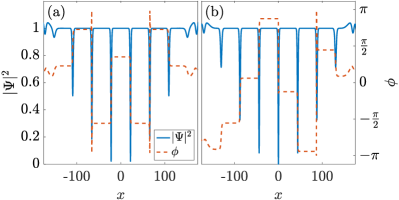
Figure 1: Left axes: Profile snapshots of the density, $|\Psi|^{2}$, at $t=150$ showcasing the generated dark solitons for (a) IP-IRP and (b) OP-IRP initial conditions. In both cases $|u|=1$ and $a=5$, resulting in three pairs of dark solitons being formed in (a) and three pairs and a central black soliton in (b). Right axes: Snapshots of the corresponding phase, $\phi$, (see legend) for (a) an IP-IRP and (b) an OP-IRP illustrating the characteristic phase-jump occurring at each of the dark soliton minima. Phase-shifts $0<\Delta\phi<\pi$ correspond to moving (gray) solitons, and the maximum phase-shift $\Delta\phi=\pi$ belongs to the black soliton centered at $x=0$ in the OP case (b).

Up to this point we have briefly reviewed the well-known results regarding the controllable generation of multiple dark solitons in homogeneous single-component settings. Below, we focus on the controllable formation of more complex solitonic entities that appear in multi-component BECs. In this latter context analytical expressions like the ones provided by Eq. (7) and Eq. (9) are, to the best of our knowledge, currently unavailable in the literature for the initial waveforms considered herein. Thus, in the following we resort to a systematic numerical investigation aiming at controlling the emergence of more complex solitonic structures consisting of multiple solitons of the DB type. In particular, we initially focus on the simplest case scenario, i.e. a two-component BEC [see Eq.(3)]. Next in our systematic progression, we consider a three-component mixture [see Eq.(2)]; finally, we turn our attention to the true spinorial BEC system [see Eqs.(LABEL:eq:spinor_hamiltonian_a)-(LABEL:eq:spinor_hamiltonian_b)]. Additionally, and also in all cases that will be examined herein, in order to initialize the dynamics, we use as initial condition for the component(s) that during the evolution will host multiple dark solitons the IRP wavefunction given by Eq. (5). Furthermore, for the component(s) that during the evolution will host multiple bright states a Gaussian pulse is used. The latter ansatz is given by

$$\Psi(x,0)=\sqrt{A}\exp\left[-\frac{1}{2}\kappa^{2}(x-X_{0})^{2}\right],$$ (10)

with $A$, $\kappa$ and $X_{0}$ denoting respectively the amplitude, the inverse width and the center of the Gaussian pulse. To minimize the emitted radiation during the counterflow process, in the trapped scenarios the following procedure is used. The multi-component system is initially relaxed to its ground state configuration. For the relaxation process we use as an initial guess Thomas-Fermi (TF) profiles for all the participating components, i.e. $\Psi(x)=\sqrt{\mu-V_{i}(x)}$. Here, $\mu$ denotes the common chemical potential assumed throughout this work for all models under consideration. It is relevant to mention in passing here that the selection of a common $\mu$ is a necessity (due to the spin-dependent interaction) in the spinor system, but not in the Manakov case (where it constitutes a simplification in order to reduce the large number of parameters in the problem). Additionally, $i=d,b$ indicates the different traps used for the participating species. In particular, the component(s) that will host during evolution dark solitons is (are) confined in a double-well potential that reads Reinhardt and Clark (1997); Theocharis et al. (2010)

$$V_{d}(x)=V(x)+G\exp\left(-x^{2}/w^{2}\right).$$ (11)

In Eq. (11), $V(x)$ is the standard harmonic potential, while $G$ and $w$ are the amplitude and width of the Gaussian barrier used. Tuning $G$ and $w$ allows us to control the spatial separation of the two condensates. We also note in passing that the choice of Eq. (11) is based on the standard way to induce the counterflow dynamics in single-component BEC experiments Weller et al. (2008); Hoefer et al. (2009). The remaining component(s) that during evolution will host bright solitons are trapped solely in a harmonic potential $V_{b}(x)=\frac{1}{2}\Omega_{b}^{2}x^{2}$, with $\Omega_{b}>\Omega$. The latter choice is made in order to reduce the initial spatial overlap between the components which, in turn, facilitates soliton generation during the dynamics. After the above-discussed relaxation process the system is left to dynamically evolve in the common harmonic potential $V(x)$ by switching off the barrier in Eq. (11), i.e. setting $G=0$, and also removing $V_{b}$ by setting $\Omega_{b}=0$.

In all cases under investigation, in order to simulate the counterflow dynamics of the relevant mixture a fourth-order Runge-Kutta integrator is employed, and a second-order finite differences method is used for the spatial derivatives. The spatial and time discretization are $\mathop{}\!\mathrm{d}x=0.1$ and $\mathop{}\!\mathrm{d}t=0.001$ respectively. Moreover, unless stated otherwise, throughout this work we fix $|u|=1$, $\Delta\phi=0$ [see Eq. (5)] and $A=1$, $\kappa=1$, $X_{0}=0$ [see Eq. (10)]. The default parameters for the trapped scenarios are $\mu_{j}=\mu=1$, (with $j$ denoting the participating components) $G=5\mu$, $w^{2}=5$, $\Omega=0.05$ and $\Omega_{b}=30\Omega$. We have checked that slight deviations from these parametric selections do not significantly affect our qualitative observations reported below. Additionally, for the spinor BEC system we also fix $g_{s}=-4.6{\times}10^{-3}$. Notice that the chosen value is exactly the ratio $\frac{a_{2}-a_{0}}{a_{0}+2a_{2}}$ that is (in the range) typically used in ferromagnetic spinor $F=1$ BEC of ⁸⁷Rb atoms Klausen et al. (2001); van Kempen et al. (2002). However, we note that the numerical findings to be presented below are not altered significantly even upon considering a spinor $F=1$ BEC of ²³Na atoms.

Finally, focusing on ⁸⁷Rb BEC systems, our dimensionless parameters can be expressed in dimensional form by assuming a transversal trapping frequency $\omega_{\perp}=2\pi\times 175$ Hz. Then all time scales must be rescaled by $8.1$ s and all length scales by $100~{}\rm{\mu m}$. This yields an axial trapping frequency $\omega_{x}\approx 2\pi\times 1.1$ Hz which is accessible by current state-of-the-art experiments Bersano et al. (2018). The corresponding aspect ratio is $\omega_{x}/\omega_{\perp}=5\times 10^{-3}$ and as such lies within the range of applicability of the 1D GP theory according to the criterion $Na^{4}_{\perp}/a^{2}a^{2}_{z}\gg 1$ Pitaevskii and Stringari (2016). Here $a_{\perp}$, and $a_{z}$ denote respectively the oscillator length in the transversal and axial direction, while $a$ is the three-dimensional $s$-wave scattering length.

III Numerical Results And Discussion

III.1 Two-Component BEC

In this section we present our findings regarding the controlled generation of arrays of DB solitons and their robust evolution in two-component BECs Becker et al. (2008); Middelkamp et al. (2011); Hamner et al. (2011); Yan et al. (2011); Hoefer et al. (2011); Yan et al. (2012). To induce the counterflow dynamics we utilize the methods introduced in Sec. II B. Before delving into the associated dynamics we should first recall that in the integrable limit, i.e. $g_{n}=1$ and $V(x)=0$, the system of Eqs. (3) admits an exact DB soliton solution. The corresponding DB waveforms read Yan et al. (2011); Biondini et al. (2016); Katsimiga et al. (2017a, b, 2018a)

$$\Psi_{d}(x,t) = \Big{[}\nu\tanh\left[\mathcal{D}\left(x-x_{0}(t)\right)\right]+i\lambda\Big{]}e^{-it},$$ (12)

$$\Psi_{b}(x,t) = \eta\operatorname{sech}\left[\mathcal{D}\left(x-x_{0}(t)\right)\right]e^{\left[ikx+i\varphi(t)\right]},$$ (13)

and are subject to the boundary conditions $|\Psi_{d}|^{2}\rightarrow 1$ and $|\Psi_{b}|^{2}\rightarrow 0$ as $|x|\rightarrow\infty$, in the dimensionless units adopted herein. In Eqs. (12)-(13) $\Psi_{d}$ ($\Psi_{b}$) is the wavefunction of the dark (bright) soliton component. In the aforementioned solutions, $\nu$ and $\eta$ are the amplitudes of the dark and the bright soliton respectively, while $\lambda$ sets the velocity of the dark soliton. Furthermore, $\mathcal{D}$ denotes the common –across components– inverse width parameter and $x_{0}(t)$, which will be traced numerically later on, refers to the center position of the DB soliton (see also our discussion below). Additionally, in the above expressions $k=\mathcal{D}\left(\lambda/\nu\right)$ is the constant wavenumber of the bright soliton associated with the DB soliton’s velocity, and $\varphi(t)$ is its phase. Inserting the solutions of Eqs. (12)-(13) in the system of Eqs. (3) leads to the following conditions that the DB soliton parameters must satisfy for the above solution to exist

$$\mathcal{D}^{2} = \nu^{2}-\eta^{2},$$ (14)

$$\dot{x}_{0} = \mathcal{D}\frac{\lambda}{\nu},$$ (15)

where $\dot{x}_{0}$ is the DB soliton velocity. Through the normalization of $\Psi_{b}$ we can connect the number of particles of the bright component, $N_{b}$, with $\eta$ and $\mathcal{D}$

$$N_{b}=\int|\Psi_{b}(x,t)|^{2}\text{d}x=\frac{2\eta^{2}}{\mathcal{D}}.$$ (16)

In the following we will use the aforementioned conditions, namely Eqs. (14)-(15), not only to verify the nature of the emergent states but also to compare the trajectories of the evolved DBs to the analytical prediction provided by Eq. (15). Moreover, by making use of Eq. (16) we will further estimate the number of particles hosted in the bright soliton component of the mixture.

The outcome of the counterflow process for different variations of the half-width $a$ of the initial IP-IRP is illustrated in Figs. 2(a)-2(f).

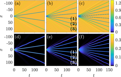
Figure 2: Spatio-temporal evolution of the density $\left|\Psi_{1}\right|^{2}$ ($\left|\Psi_{2}\right|^{2}$) of the first (second) component upon varying the half-width $a$ of the initial IRP. From left to right $a=3$, $a=5$ and $a=7$, allowing the generation of four [(a)-(d)], six [(b)-(e)], and ten [(c)-(f)] DB solitons, respectively. In all cases, top (bottom) panels illustrate the formation of dark (bright) solitons in the first (second) component of the two-component system. Labels $(1)$-$(3)$ introduced in panels $(b)$, $(e)$ number the DB solitons discussed in Table 1.

In particular, in all cases depicted in this figure, the spatio-temporal evolution of the densities, $|\Psi_{j}|^{2}$ (with $j=1,2$), of both components for propagation times up to $t=150$ is presented. It is found that from the very early stages of the dynamics the interference fringes in the first component evolve into several dark soliton states being generated in this component. E.g. four dark solitons can be readily seen in Fig. 2(a) for $a=3$. The nucleation of these dark states leads in turn to the emergence, via the confinement of the spreading Gaussian pulse, also of four bright solitons in the second component of the binary mixture [Fig. 2(d)]. The latter bright waveforms are created in each of the corresponding dark minima, and are subsequently waveguided by their dark counterparts. The robust propagation of the newly formed array of DB solitons is illustrated for times up to $t=150$. Importantly here, we were able to showcase that by tuning the half-width of the initial IRP a controllable formation of arrays of DB solitons can be achieved. In particular, it is found that upon increasing the initial half-width of the IP-IRP leads to a larger number of DB solitons being generated. Indeed, as shown in Figs. 2(b) and 2(e) six DB states are formed for $a=5$, while for $a=7$ the resulting array consists of ten DB solitons as illustrated in Figs. 2(c) and 2(f). We should remark also here that since an IP-IRP is utilized only an even number of DB solitons is expected and indeed observed in all of the aforementioned cases. This result is in line with the analytical predictions discussed in the single-component scenario [see also Eq. (7)].

Moreover, to verify that indeed the entities formed are DB solitons we proceed as follows. Firstly, upon fitting it is confirmed that the evolved dark and bight states have the standard $\tanh$- and $\rm{sech}$-shaped waveform respectively [see Eqs. (12)-(13)]. Then, by monitoring during evolution a selected DB pair we measure the amplitudes $\nu$ and $\eta$ of the dark and the bright constituents, respectively. Having at hand the numerically obtained amplitudes we then use the analytical expressions stemming from the single DB soliton solution, namely Eqs. (14)-(16). In this way estimates of the corresponding DB trajectory as well as the number of particles, $N_{b}$, hosted in the selected bright soliton are extracted. Via the aforementioned procedure and e.g. for the closest to the origin ($x=0$) right moving DB solitary wave labeled as (1) and shown in Figs. 2(b)-2(e) it is found that $N_{b}=0.3611$ while the numerically obtained value is $N^{num}_{b}=0.3607$. Notice that the deviation between the semi-analytical calculation and the numerical one is less than $1\%$. To have access to $N^{num}_{b}$ we simply integrated $|\Psi_{2}|^{2}$ within a small region around the center of the bright part of the selected DB pair. Additionally, for the same DB pair $\dot{x}_{0}=0.1467$ while $\dot{x}^{num}_{0}=0.1495$.

After confirming that all entities illustrated in Figs. 2(a)-2(f) are indeed DB solitons, with each of the resulting DBs following the analytical predictions of Eqs. (14)-(16), we next consider different parametric variations. In particular, we will investigate modifications in the DB soliton characteristics when the number of the nucleated DB states is held fixed. To this end, below we fix $a=5$ and we then vary within the interval $[0.5,2]$ one of the following parameters at a time: $|u|$, $A$, $\kappa$.

Before proceeding, two important remarks are of relevance at this point. (i) Fixing $a=5$ is not by itself sufficient to a priori ensure that a fixed number of DB solitons will be generated via the interference process. This is due to the fact that the number of solitons formed is proportional to $a$ and $|u|$ as detected by Eq. (7). This is the reason for restricting ourselves to the aforementioned interval in terms of $|u|$ ($|u|\in[0.5,2]$). This selection leads to the formation of an array consisting of only six DB solitons like the ones shown in Figs. 2(b) and 2(e) for $A=\kappa=1$. (ii) Additionally here, variations of either $A$, or $\kappa$ could in principle affect the bright soliton formation, however we have not found this to be the case in our intervals of consideration.

Taking advantage of the symmetric formation of these six DB structures in the analysis that follows we will focus our attention to the three, i.e. (1), (2), and (3), right moving with respect to $x=0$ DB solitons shown in Figs. 2(b) and 2(e).

[0.5, 2]

$\left|u\right|\uparrow$

$A\uparrow$

$\kappa\uparrow$

DB

$\nu$

$\eta$

$D$

$n_{b}$

$\dot{x}_{0}$

$\nu$

$\eta$

$D$

$n_{b}$

$\dot{x}_{0}$

$\nu$

$\eta$

$D$

$n_{b}$

$\dot{x}_{0}$

(1)

$\uparrow$

$\uparrow$

$\uparrow$

$\uparrow$

$\uparrow$

$\downarrow$

$\uparrow$

$\downarrow$

$\downarrow$

$\downarrow$

$\uparrow$

$\downarrow$

$\uparrow$

$\downarrow$

$\downarrow$

(2)

$\uparrow$

$\uparrow$

$\uparrow$

$\uparrow$

$\uparrow$

$\downarrow$

$\uparrow$

$\downarrow$

$\downarrow$

$\downarrow$

$\uparrow$

$\downarrow$

$\uparrow$

$\downarrow$

$\downarrow$

(3)

$\uparrow$

$\uparrow$

$\uparrow$

$\downarrow$

$\uparrow$

$\downarrow$

$\uparrow$

$\downarrow$

$\uparrow$

$\downarrow$

$\uparrow$

$\downarrow$

$\uparrow$

$\uparrow$

$\downarrow$

Table 1: Changes in the DB soliton characteristics upon considering different variations of the systems’ parameters for fixed $a=5$. Here, $(1)$ [$(3)$] refers to the most inner [outer] DB solitons [see Figs. 2(b) and 2(e)]. The top row indicates the distinct variations, namely of each $|u|$, $A$, and $\kappa$, performed separately within the interval $[0.5,2]$. The second row contains the soliton characteristics such as the dark, $\nu$, and bright, $\eta$, amplitudes. Also shown are the inverse width, $\mathcal{D}$, the normalized number of particles, $n_{b}$, hosted in each of the bright solitons formed in the second component of the mixture, and the velocity, $\dot{x}_{0}$, of the DB pair. $\uparrow$ ($\downarrow$) arrows indicate an increase (decrease) of the corresponding quantity.

The effect that different parametric variations have on the characteristics of these three DB solitons are summarized in Table 1. In particular in this table, the arrow $\uparrow$ ($\downarrow$) indicates an increase (decrease) of the corresponding soliton characteristic as one of the parameters $|u|$, $A$ and $\kappa$ is increased within the chosen interval. In general, it is found that as the amplitude, $|u|$, of the initial IP-IRP increases the amplitudes, $\nu$, $\eta$, of all three DB structures increase as well [see the second column in Table 1]. Also, the resulting DB states are found to be narrower (larger inverse width $\mathcal{D}$) and faster (larger $\dot{x}_{0}$). However, the normalized number of particles, $n_{b}$, hosted in each of the bright soliton constituents is found to increase for the two innermost DB states [i.e. (1) and (2)] while it decreases for the outer one [i.e. (3)]. For instance, for the inner DB wave labeled (1) shown in the first column of Table 1, $n_{b}$ is found to be $n_{b}=0.196$ for $|u|=0.5$, while $n_{b}=0.204$ for $|u|=1$. Thus, the symbol $\uparrow$ is used to describe the increasing tendency of $n_{b}$ [see the second column of Table 1]. We defined $n_{b}$ according to $n_{b}=N^{num}_{b}/N_{2}$ with $N_{2}=\int|\Psi_{2}|^{2}\text{d}x$ being the total number of particles in the second component of the binary mixture. For comparison here, for the outer DB soliton labeled (3) $n_{b}=0.092$ for $|u|=0.5$ while $n_{b}=0.075$ for $|u|=1$ and thus a symbol $\downarrow$ is introduced [see again the second column in Table 1].

On the contrary upon increasing the amplitude, $A$, of the initial Gaussian pulse [see Eq. (10)] the amplitudes of all dark (bright) solitons for all three DB pairs decrease (increase), thus a decrease of the corresponding inverse width results in wider and slower soliton pairs [see the third column in Table 1]. Moreover, $n_{b}$ is found to decrease for the two inner DB pairs while it increases for the outer one. Variations of the inverse width, $\kappa$, of the Gaussian pulse have more or less the opposite to the above-described effect. As $\kappa$ increases, the resulting dark (bright) states have larger (smaller) amplitudes for all three DB pairs but the solitons are narrower and slower [see the fourth column in Table 1]. Recall that narrower does not directly imply faster states since the amplitude of the generated dark solitons is also involved [see Eqs. (14), (15)]. Also in this case $n_{b}$ increases for the outer DB pair [see the fourth column in Table 1]. Finally, we also considered different displacements, $X_{0}$, of the initial Gaussian pulse within the interval $[0,7.5]$. A behavior similar to the aforementioned $\kappa$ variation is observed. However, the produced solitons are found to be asymmetric for $X_{0}\neq 0$ due to the asymmetric positioning of the two components. On the other hand, for $X_{0}\geq a$ ($a=5$) we never observe DB soliton generation.

Having discussed in detail the homogeneous system, we next turn our attention to the harmonically confined one [see Eq. (3)]. Recall that in this case the initial guesses used for both components of the binary mixture are TF profiles. The first component is initially confined in the double-well potential $V_{d}(x)$ with the width $w$ of the barrier controlling the spatial separation of the two parts of the condensate [see Eq. (11)]. The corresponding second component is in turn trapped in the harmonic potential $V_{b}(x)$ (see Sec. II B). After relaxation the two-component system is left to dynamically evolve in the common parabolic trap $V(x)$.

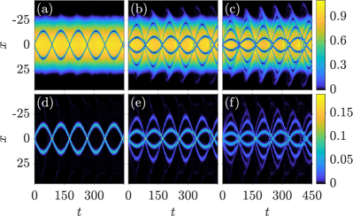
Figure 3: Spatio-temporal evolution of the density $\left|\Psi_{1}\right|^{2}$ ($\left|\Psi_{2}\right|^{2}$) of the first (second) component in the trapped scenario upon varying the width of the double-well barrier $w$ used for the preparation of the initial state. From left to right $w^{2}=1$, $w^{2}=5$ and $w^{2}=10$, allowing the generation of two [(a)-(d)], four [(b)-(e)], and six [(c)-(f)] DB solitons respectively. In all cases, top (bottom) panels illustrate the formation of dark (bright) solitons in the first (second) component of the two-component system.

In line with our findings for the homogeneous setting, also here a desirable number of DB solitons can be achieved by properly adjusting either $w$ or the chemical potentials $\mu_{i}$ (with $i=1,2$) of the binary mixture. Note that in this latter case, the amplitude of the system is directly related to $\mu$ [see Eq. (7)]. In both cases, it is found that an increase of $w$ or $\mu$ results to more DB solitons being generated. In particular, Figs. 3(a)-3(c) [Figs. 3(d)-3(f)] illustrate the dynamical evolution of the density, $|\Psi_{1}|^{2}$ ($|\Psi_{2}|^{2}$), of the first (second) component of the mixture upon increasing $w$. An array consisting of two, four and six DB solitons pairs can be observed for $w^{2}=1$, $w^{2}=5$ and $w^{2}=10$ respectively. In all cases depicted in this figure the DB states are formed from the very early stages of the dynamics. After their formation the states begin to oscillate within the parabolic trap. Monitoring their propagation for evolution times up to $t=450$, it is found that while coherent oscillations are observed for the two DB case [see Figs. 3(a), 3(d)], this picture is altered for larger DB soliton arrays. In the former case measurements of the oscillation frequency, $\omega_{osc}$, verify that it closely follows the analytical predictions for the single DB soliton. Namely, $\omega_{osc}=\Omega^{2}\left(\frac{1}{2}-\frac{\chi}{\chi_{0}}\right)$, with $\chi=N_{2}/\sqrt{\mu}$ and $\chi_{0}=8\sqrt{1+\left(\frac{\chi}{4}\right)^{2}}$ Busch and Anglin (2001); Yan et al. (2011). For instance, our semi-analytical calculation stemming from the aforementioned theoretical prediction gives $\omega_{osc}=34.3\times 10^{-3}$, while direct measurements from our numerical simulations provide $\omega_{osc}^{num}=35.3\times 10^{-3}$. This represents a $3\%$ discrepancy, which can be attributed to the interaction of the solitons both with one another but also with the background excitations, with the latter having the form of sound waves. Additionally, it should be noted that the theoretical prediction is valid in the large $\mu$ limit (which may be partially responsible for the relevant discrepancy). However, for larger DB soliton arrays the number of collisions is higher and the background density is more excited, as can be deduced by comparing Figs. 3(a), 3(d) to Figs. 3(b), 3(e) and Figs. 3(c), 3(f). Importantly here the generated DB states are of different mass and thus each DB soliton oscillates with its own $\omega_{osc}$. It is this mass difference that results in the progressive “dephasing” observed during evolution. Notice also that in all cases illustrated in the aforementioned figures the outer (faster) DB solitons are the ones that are affected the most. The above effect is enhanced for larger initial separations $w$ [compare Figs. 3(b), 3(e) to Figs. 3(c), 3(f)], leading to discrepancies up to $11.6\%$ between $\omega_{osc}$ and $\omega^{num}_{osc}$ observed for the outermost DB pair shown in Figs. 3(c), 3(f).

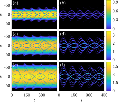
Figure 4: Spatio-temporal evolution of the density $\left|\Psi_{1}\right|^{2}$ ($\left|\Psi_{2}\right|^{2}$) of the first (second) component in the trapped scenario upon varying the chemical potential $\mu$ while fixing $w^{2}=5$. From top to bottom $\mu=1$, $\mu=3$ and $\mu=5$, leading to the emergence of four [(a)-(b)], six [(c)-(d)], and eight [(e)-(f)] DB solitons respectively. In all cases, left (right) panels illustrate the formation of dark (bright) solitons in the first (second) component of the two-component system.

As mentioned above, besides $w$ also the chemical potential $\mu$ serves as a controlling parameter. Indeed, by inspecting the spatio-temporal evolution of the densities, $|\Psi_{j}|^{2}$ (with $j=1,2$), shown in Figs. 4(a)-4(f) for fixed $w^{2}=5$ it becomes apparent that increasing $\mu$ leads to an increased number of DB solitons being generated. Four, six and eight DB solitons are seen to be nucleated for $\mu=1$, $\mu=3$ and $\mu=5$ respectively, and to propagate within the BEC medium for long evolution times. Notice that Figs. 4(a), 4(b) are the same as Figs. 3(b), 3(e). Increasing the system size reduces the impact that the radiation expelled (when matter-wave interference takes place) has on the resulting DB states, as can be deduced by comparing Figs. 4(c), 4(d) to Figs. 3(c), 3(f). Indeed, further measurements of $\omega_{osc}$ reveal that the maximum discrepancy observed for the outermost DB solitons when $\mu=1$ [see Figs. 4(a),4(b)] is of about $8.5\%$, while upon increasing $\mu$ the discrepancy is significantly reduced. The latter reduction is attributed to the fact that for larger $\mu$ the asymptotic prediction of $\omega_{osc}$ is progressively more accurate. More specifically, for $\mu=5$ we obtain a discrepancy of only $0.3\%$ for the third, with respect to $x=0$, DB soliton pair shown in Figs. 4(e), 4(f). Yet still, the emergent DB states have different periods of oscillation, leading in turn to several collision events taking place during evolution. Nevertheless, in all cases presented above a common feature of the solitary waves is that they survive throughout our computational horizon.

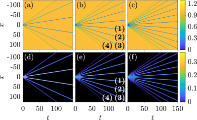
Figure 5: Spatio-temporal evolution of the density $|\Psi_{+1}|^{2}$ ($|\Psi_{-1}|^{2}$) of the $m_{F}={+1}$ ($m_{F}={-1}$) component upon varying the half-width $a$ of the initial IRP. From left to right $a_{+1}=a_{0}=3$, $a_{+1}=a_{0}=5$ and $a_{+1}=a_{0}=7$, resulting in the nucleation of six [(a), (d)], eight [(b), (e)], and twelve [(c), (f)] DDB solitons respectively. In all cases, top (bottom) panels illustrate the formation of dark (bright) solitons in the $m_{F}={+1}$ ($m_{F}={-1}$) component of the three-component system. Since the evolution of the $m_{F}={0}$ component is the same as the one depicted for the $m_{F}={+1}$, only the two components that differ from one another are illustrated. The labels, (1)-(4) introduced in [(b), (e)] number the DDB solitons that are discussed in Table 2.

III.2 Three-component BEC mixtures

Now, we increase the complexity of the system by adding yet another component to the previously discussed two-component mixture. Namely we consider a three-component mixture consisting of three different hyperfine states of the same alkali isotope such as ⁸⁷Rb. We aim at revealing the DB soliton complexes that arise in such a system and their controllable formation via the interference processes introduced in Sec. II.2. From a theoretical point of view, such a three-component BEC mixture is described by a system of three coupled GPEs (see Eqs. (2) in Sec. II.1), i.e., one for each of the participating $m_{F}=+1,0,-1$ components.

To begin our analysis, we start with the integrable version of the problem at hand. Namely, we fix $g_{n}=1$ and we set $V(x)=0$ in the corresponding Eqs. (2). This homogeneous mixture admits exact solutions in the form of DDB and DBB solitons as it was rigorously proven via the inverse scattering method Biondini et al. (2016). In the following, we will attempt to produce in a controlled fashion arrays consisting of these types of soliton compounds. We further note that in the numerical findings to be presented below the abbreviations in the form XYZ (with X,Y,Z=D or B) reflect the $m_{F}=+1,0,-1$ order. E.g. a DDB abbreviation indicates that dark solitons are generated in the $m_{F}=+1,0$ components while bright solitons are generated in the $m_{F}=-1$ component of the mixture.

As it was done in the two-component setting, in order to generate a DDB configuration the counterflow dynamics is performed by two of the participating hyperfine components. Recall that dark solitons in each hyperfine state emerge via the destructive interference that takes place at the origin where the two spatially separated sides of the initial IP-IRP collide. Specifically, the initial ansatz used for the $m_{F}=+1,0$ states is provided by Eq. (5) and the corresponding ansatz for the $m_{F}=-1$ component is the Gaussian of Eq. (10). It turns out that we can again tailor the number of nucleated DDB solitons by manipulating the half-width, $a_{m_{F}}$ (with ${m_{F}}=+1,0$), of the initial IP-IRP. To showcase the latter in Figs. 5(a)-5(f) we present the outcome of the distinct variations of $a_{m_{F}}$. Notice that as $a_{m_{F}}$ increases arrays consisting of a progressively larger number of DDB solitons are formed. Namely, $a_{+1}=a_{0}=3$ results in an array of six DDB solitons [Figs. 5(a), 5(d)]. Accordingly, when $a_{+1}=a_{0}=5$ the nucleation of eight DDB waveforms is observed [see Figs. 5(b), 5(e)], while twelve such states occur for $a_{+1}=a_{0}=7$ [Figs. 5(c), 5(f)]. In all of the above cases the spatio-temporal evolution of the densities $|\Psi_{+1}|^{2}$, and $|\Psi_{-1}|^{2}$, are shown in the top and bottom panels of Fig. 5 respectively. The resulting propagation of the ensuing DDB states is monitored for evolution times up to $t=150$. Moreover, only the $m_{F}=\pm 1$ components are depicted in the aforementioned figure. This is due to the fact that the evolution of the $m_{F}=0$ component is essentially identical to the one shown for the $m_{F}=+1$ component.

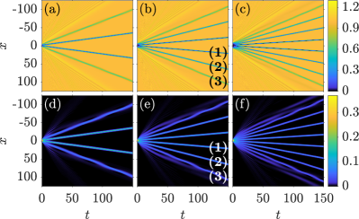
Figure 6: Same as in Fig. 5 but showcasing the generation of DBB solitons. In this case, from left to right $a_{+1}=3$, $a_{+1}=5$ and $a_{+1}=7$, allowing the generation of four [(a)-(d)], six [(b)-(e)], and eight [(c)-(f)] DBB solitons respectively. The labels, (1)-(3) introduced in [(b), (e)] number the DBB solitons that are discussed in Table 3.

[0.5 , 2]

$\left|u_{0}\right|\uparrow$

$A_{-1}\uparrow$

$\kappa_{-1}\uparrow$

DDB

$\nu_{+1}$

$\nu_{0}$

$\eta_{-1}$

$\mathcal{D}$

$n_{b}$

$\dot{x}_{0}$

$\nu_{+1}$

$\nu_{0}$

$\eta_{-1}$

$\mathcal{D}$

$n_{b}$

$\dot{x}_{0}$

$\nu_{+1}$

$\nu_{0}$

$\eta_{-1}$

$\mathcal{D}$

$n_{b}$

$\dot{x}_{0}$

(1)

$\uparrow$

$\uparrow$

$\uparrow$

$\uparrow$

$\uparrow$

$\uparrow$

$\downarrow$

$\downarrow$

$\uparrow$

$\downarrow$

$\downarrow$

$\updownarrow$

$\uparrow$

$\uparrow$

$\downarrow$

$\uparrow$

$\downarrow$

$\downarrow$

(2)

$\uparrow$

$\uparrow$

$\uparrow$

$\uparrow$

$\uparrow$

$\uparrow$

$\downarrow$

$\downarrow$

$\uparrow$

$\downarrow$

$\downarrow$

$\updownarrow$

$\uparrow$

$\uparrow$

$\downarrow$

$\uparrow$

$\downarrow$

$\downarrow$

(3)

$\uparrow$

$\uparrow$

$\uparrow$

$\uparrow$

$\downarrow$

$\uparrow$

$\downarrow$

$\downarrow$

$\uparrow$

$\downarrow$

$\uparrow$

$\updownarrow$

$\uparrow$

$\uparrow$

$\downarrow$

$\uparrow$

$\uparrow$

$\downarrow$

(4)

$\uparrow$

$\uparrow$

$\uparrow$

$\uparrow$

$\downarrow$

$\uparrow$

$\downarrow$

$\downarrow$

$\uparrow$

$\downarrow$

$\uparrow$

$\updownarrow$

$\uparrow$

$\uparrow$

$\uparrow$

$\uparrow$

$\uparrow$

$\downarrow$

Table 2: Changes in the DDB soliton characteristics upon considering different variations of the systems’ parameters and monitoring the four right moving DDB solitons generated for fixed $|u_{+1}|=1$ and $a_{+1}=a_{0}=5$. Here, $(1)$ [$(4)$] refers to the inner [outer] most DDB state [see Figs. 5(b) and 5(e)]. The top row indicates the distinct variations, namely $|u_{0}|$, $A_{-1}$, and $\kappa_{-1}$, performed within the interval $[0.5,2]$. The second row contains the soliton characteristics, i.e. the dark, $\nu_{+1,0}$, and bright, $\eta_{-1}$, amplitudes, the common inverse width, $\mathcal{D}$, the normalized number of particles, $n_{b}$, hosted in the bright soliton component and the velocity, $\dot{x}_{0}$, of the DDB pair. $\uparrow$ arrows ($\downarrow$) indicate an increase (decrease) of the corresponding quantity. $\updownarrow$ arrows indicate that within the above interval a non-monotonic tendency of the respective quantity is observed.

The same overall picture is qualitatively valid for the corresponding DBB soliton formation. Note that in contrast to the DDB nucleation, to generate DBB soliton arrays the counterflow dynamics is featured solely by one of the hyperfine components which as per our choice is the $m_{F}={+1}$ one. The remaining two hyperfine components, namely $m_{F}={0,-1}$ share the same Gaussian-shaped initial profile. In Figs. 6(a)-6(f) the formation of four, six and eight DBB soliton complexes is shown for $a_{+1}=3$, $a_{+1}=5$ and $a_{+1}=7$ respectively. Notice that the number of the generated DBB states appears to be lower when compared to the DDB solitons formed for the same value of $a_{+1}$. For instance, four DBB solitons are formed for $a_{+1}=3$ [Figs. 6(a), 6(d)] while the corresponding DDB soliton count is six [Figs. 5(a), 5(d)]. The observed difference between the number of nucleated DBB and DDB states can be intuitively understood as follows. For a DDB production the total number of particles is $N=2990$ while for a DBB one is $N=1498$ e.g. for the case examples presented in Figs. 5(a), 5(d) and Figs. 6(a), 6(d) respectively. Recall that in our simulations we fix the chemical potential and thus $N$ is a free parameter. The significantly lower number of particles in a DBB nucleation process stems from the fact that two of the participating components have a Gaussian initial profile and as such host fewer particles. This decrease of the system size for a DBB realization when compared to a DDB one may be partially responsible for the observed decreased DBB soliton count. Moreover, in the DDB case the presence of two components (namely $m_{F}=+1,0$ components each one characterized by an amplitude $|u|$) with a finite background leads to a total amplitude $|u_{eff}|\approx 2|u|$. Thus, as dictated by Eq. (7), the number of solitons is expected to be higher as well. Further adding to the above, for a DBB formation only one component develops, via interference, dark solitons. These dark solitons are, in turn, responsible for the trapping of bright solitons in the other two hyperfine components. However, since two components develop bright solitons effectively the number of particles that have to be sustained by each effective dark well increases. As such in the DBB case, the system prefers to develop fewer but also wider and deeper dark solitons than in the DDB process; this is also inter-related with the smaller counterflow induced momentum in the DBB cse. These deeper dark solitons can in turn efficiently trap and waveguide the resulting also fewer bright solitons. The above intuitive explanation is fairly supported by our findings. Indeed, both the dark and the bright solitons illustrated in Figs. 6(a), 6(d) appear to be wider having also larger amplitudes when compared to the ones formed in the DDB interference process shown in Figs. 5(a), 5(d).

In all cases presented in Figs. 5(a)-5(f) and Figs. 6(a)-6(f), we were able to showcase upon fitting that the evolved dark and bright states have the standard $\tanh$- and $\operatorname{sech}$-shaped waveform respectively [see Eqs. (12)-(13)]. Moreover, following the procedure described in the two-component setting (see Sec. III.1), we verified that the number of particles hosted in each of the bright solitons formed follows Eq. (16), with the common inverse width, $\mathcal{D}$, satisfying the generalized conditions

$$\mathcal{D}^{2} = \nu_{j}^{2}+\nu_{k}^{2}-\eta_{l}^{2},$$ (17)

$$\mathcal{D}^{2} = \nu_{j}^{2}-\eta_{k}^{2}-\eta_{l}^{2},$$ (18)

for the DDB and the DBB cases respectively. The indices $j,k,l$ in the above expressions denote the three (distinct) hyperfine components. As a case example, for one of the DDB states shown in Figs. 5(b), 5(e) $N^{num}_{b}=0.3715$ while the semi-analytical prediction gives $N_{b}=0.3721$. Notice that the deviation is again smaller than $1\%$.

As a next step, we attempt to appreciate the effect that different initial configurations have on the characteristics of the resulting DDB and DBB soliton compounds. Our findings are summarized in Tables 2 and 3 respectively. Specifically, for a DDB nucleation process $|u_{+1}|=1$ and $a_{+1}=a_{0}=5$ are held fixed. The remaining parameters are varied (one of them at a time) within the interval $[0.5,2]$. The above selection leads to the appearance of eight DDB solitons symmetrically formed around the origin as already illustrated in Figs. 5(d), 5(e). Exploiting this symmetric formation only the four, i.e. (1)-(4), right moving DDB solitons indicated in Figs. 5(d), 5(e) are monitored and shown in Table 2.

[0.5 , 2]

$\left|u_{+1}\right|\uparrow$

$A_{0}\uparrow$

$\kappa_{0}\uparrow$

DDB

$\nu_{+1}$

$\eta_{0}$

$\eta_{-1}$

$\mathcal{D}$

$n_{0}$

$n_{-1}$

$\dot{x}_{0}$

$\nu_{+1}$

$\eta_{0}$

$\eta_{-1}$

$\mathcal{D}$

$n_{0}$

$n_{-1}$

$\dot{x}_{0}$

$\nu_{+1}$

$\eta_{0}$

$\eta_{-1}$

$\mathcal{D}$

$n_{0}$

$n_{-1}$

$\dot{x}_{0}$

(1)

$\uparrow$

$\uparrow$

$\uparrow$

$\uparrow$

$\uparrow$

$\uparrow$

$\uparrow$

$\downarrow$

$\uparrow$

$\downarrow$

$\downarrow$

$\downarrow$

$\downarrow$

$\downarrow$

$\uparrow$

$\downarrow$

$\uparrow$

$\uparrow$

$\downarrow$

$\downarrow$

$\updownarrow$

(2)

$\uparrow$

$\uparrow$

$\uparrow$

$\uparrow$

$\uparrow$

$\uparrow$

$\uparrow$

$\downarrow$

$\uparrow$

$\downarrow$

$\downarrow$

$\downarrow$

$\downarrow$

$\downarrow$

$\uparrow$

$\downarrow$

$\uparrow$

$\uparrow$

$\updownarrow$

$\uparrow$

$\updownarrow$

(3)

$\uparrow$

$\uparrow$

$\uparrow$

$\uparrow$

$\downarrow$

$\downarrow$

$\uparrow$

$\downarrow$

$\uparrow$

$\downarrow$

$\downarrow$

$\uparrow$

$\uparrow$

$\downarrow$

$\uparrow$

$\downarrow$

$\uparrow$

$\uparrow$

$\updownarrow$

$\updownarrow$

$\updownarrow$

Table 3: Same as Table 2 but for the three right moving DBB solitons generated for fixed $a_{+1}=5$. $(1)$ [$(3)$] denotes the inner [outer] most DBB structure shown in Figs. 6(b) and 6(e). Other parameters used are $A_{-1}=\kappa_{-1}=1$.

It becomes apparent, by comparing the DDB results of Table 2 with the ones found in the two-component scenario (see Table 1), that the inclusion of an extra $m_{F}=+1$ component prone to host dark solitons leads to the following comparison of the resulting soliton characteristics. As $|u_{0}|$ is increased within the interval $[0.5,2]$, all the generated DDB states appear to be faster and narrower (see second column in Table 2). Additionally, larger amplitudes are observed for all the solitons in all the three hyperfine components. The same qualitative results were also found in the relevant variation but for the two-component system (see second column in Table 1). It is important to stress at this point that further increase of $|u_{0}|$ and/or different initial values of $|u_{+1}|$, can lead to a change in the number of states generated as suggested also by Eq. (7). This is the reason for limiting our variations to the aforementioned interval. However, our findings for choices of $|u_{+1}|\neq|u_{0}|$ suggest that, given the same half-width $a_{+1}=a_{0}$, the number of nucleated DDB solitons will be determined by the larger $|u_{m_{F}}|$ value.

On the contrary, upon varying the amplitude, $A_{-1}$, of the initial Gaussian pulse the impact of the additional $m_{F}=+1$ component is imprinted on the velocity outcome of the resulting DDB solitons (see third column in Table 2). Indeed, as $A_{-1}$ increases a uniquely defined tendency of the velocity of the resulting states cannot be inferred at least within the interval of interest here. This result differs from the systematic overall decrease of the DB soliton velocity observed in the two-component scenario (see third column in Table 1). Notice also that all the remaining soliton characteristics here are similar to the ones found in the two-component scenario (compare the third column in Tables 2 and 1, respectively). Additionally, the presence of the extra $m_{F}=+1$ component leads to no modification on the observed DDB soliton characteristics when considering variations of the inverse width, $\kappa_{-1}$, of the Gaussian pulse (see fourth column in Table 2). Namely, for increasing $\kappa_{-1}$ all the resulting DDB states are narrower and slower. An outcome that was also found in this type of variation but in the two-component setting (see fourth column in Table 1).

Next we will check the same diagnostics but for the DBB nucleation process. Along the same lines, the initial parameters used for a DBB realization are $A_{0}=\kappa_{0}=1$ and $a_{+1}=5$ [as per Eq. (10) and Eq. (5) respectively]. This choice, results in the six DBB solitons illustrated in Figs. 6(d), 6(e). Again due to symmetry only the three, (1)-(3), right moving states indicated in Figs. 6(d), 6(e) are monitored in Table 3. When comparing the relevant findings presented in Table 3 to those shown in Table 1 the following conclusions can be drawn. For increasing $|u_{+1}|$ the generated DBB solitons are found to be narrower and faster similarly to the evolved DB states observed in the two-component scenario (see second column in Table 1). Alterations occur only upon varying the characteristics of the initial Gaussian pulse. In particular, the effect of adding an extra bright component upon increasing the amplitude, $A_{0}$, of the initial Gaussian pulse is the observed increased amplitude of all bright solitons formed in this component (see third column in Table 3). Yet, all the resulting DBB states are found to be wider and slower for increasing $A_{0}$, an outcome which is similar to that found in the two-component setting (see third column in Table 1). Lastly, upon increasing $\kappa_{0}$ the impact that the extra $m_{F}=0$ component has on the resulting DBB solitons is the following (see fourth column in Table 3). Besides the observed decreased amplitude of all bright solitons formed in this component, the outermost DBB states, i.e. (2), (3), are the ones that are affected the most. Notice that a non-monotonic response of the normalized number of particles, $n_{0}$, hosted in this $m_{F}=0$ component is found as $\kappa_{0}$ increases within the interval $[0.5,2]$. Additionally, the velocity of all three DBB solitons shows a non-monotonic tendency as $\kappa_{0}$ is increased. It is relevant to note that this result is in contrast to the decrease observed in the two-component scenario (see fourth column in Table 1).

It is worth commenting at this point that in both of the above-discussed processes we also considered variations of the relevant in each case $a_{m_{F}}$. Recall that $a_{+1,0}$ and $a_{+1}$ are the associated half-widths of the initial IP-IRP for a DDB and DBB nucleation process respectively. In particular, by fixing all parameters to their default values (see here Sec. II.2) we varied the relevant $a_{m_{F}}$ within the interval $[1,10]$. The general conclusion for such a variation, in both processes, is that increasing $a_{m_{F}}$ results to more states which become narrower and slower as their number is increased. Differences here, mostly refer to the relevant amplitudes of the resulting solitons and the normalized number of particles hosted in each bright soliton constituent. Importantly, and referring solely to the DDB process, it is found that given the same initial amplitude, $|u_{m{{}_{F}}}|$, the number of solitons generated depends on the smallest initial $a_{m_{F}}$. For this latter case ($a_{+1}\neq a_{0}$) a spatially modulated density background occurs for the components hosting the dark states. Finally, and also in both processes we were able to verify that for displacements, $X_{0}$, of the initial Gaussian pulse $X_{0}\geq a$ generation of DDB and DBB solitons is absent. This is in line with our findings in the two-component system.

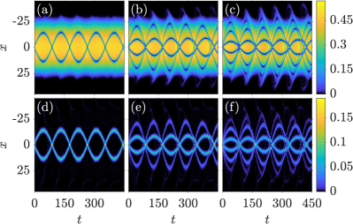
Figure 7: Evolution of the densities $|\Psi_{+1}|^{2}$, $|\Psi_{-1}|^{2}$ showcasing the generated DDB solitons in a harmonic trap with $\Omega=0.05$. Increasing the width $w$ of the double-well barrier allows the generation of DDB soliton arrays consisting of two [(a), (b)], four [(c), (d)] and six [(e), (f)] DDB solitons respectively for $w^{2}=1$, $w^{2}=5$ and $w^{2}=10$. In all cases top (bottom) panels illustrate the formation of dark (bright) solitons in the $m_{F}=+1$ ($m_{F}=-1$) component. Since the evolution of the $m_{F}=0$ component is identical to the one shown for the $m_{F}=+1$ component it is omitted.

We now turn to the trapped three-component DDB and DBB case, in analogy with the corresponding two-component one. As in the latter, for the systematic production of multiple DDB and DBB solitons we use as a control parameter the width, $w$, of the double-well potential [see Eq. (11)]. Figures 7(a)-7(f) illustrate the formation of two, four and six DDB solitons for $w^{2}=1$, $w^{2}=5$ and $w^{2}=10$ respectively. In all cases presented in this figure top (bottom) panels depict the evolution of the density, $|\Psi_{+1}|^{2}$, ($|\Psi_{-1}|^{2}$) of the $m_{F}=+1$ ($m_{F}=-1$) component. Notice the close resemblance of the dynamical evolution of the DDB states when compared to the relevant evolution of the DB soliton arrays shown in Figs. 3(a)-3(f). We remark here, that the above-observed evolution holds equally for the corresponding DBB states (results not shown here for brevity).

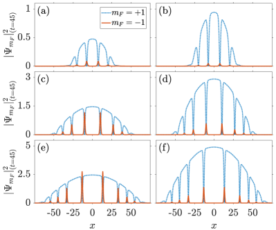
Figure 8: Profile snapshots of the density $\left|\Psi_{m_{F}}\right|^{2}$ with $m_{F}=\pm 1$ at $t=45$, illustrating the generated DDB (left) and DBB (right) solitons in the trapped scenario. In all cases $w^{2}=5$ and we vary the corresponding chemical potential. From top to bottom $\mu=1$, $\mu=3$ and $\mu=5$, resulting in turn to four [(a)-(b)], six [(c)-(d)], and eight [(e)-(f)] DDB-DBB solitons respectively. The $m_{F}=0$ component is omitted since it shows the same profile as the $m_{F}=+1$ ($m_{F}=-1$) for the DDB (DBB) nucleation process.

Furthermore, below we briefly report on the systematic production of the desired number of DDB and DBB solitons upon varying the common chemical potential $\mu$ of the confined three-component system. In Figs. 8(a)-8(f) a direct comparison of the resulting DDB and DBB soliton compounds is provided for three different values of $\mu$. Evidently, the number of DDB and DBB soliton complexes generated in each different initialization is exactly the same and as expected, it increases for increasing $\mu$. E.g for $\mu=3$ illustrated in Figs. 8(c) and 8(d) for the DDB and DBB processes respectively, the nucleated states at $t=45$ are six. Note also, that in all cases the $m_{F}=0$ component overlaps either with $m_{F}=+1$ component (DDB nucleation process) or with the $m_{F}=-1$ (DBB nucleation process) and as such it is not shown in the relevant profiles. Concluding, the dynamical evolution of both types of soliton arrays is qualitatively the same and closely resembles the one observed in the two-component setting. Also, in all the different parametric variations and for both nucleation processes studied above, the resulting arrays of DDB and DBB solitons remain robust, while oscillating and colliding with one another, for evolution times up to $t=450$ that we have checked.

III.3 Spinor BEC

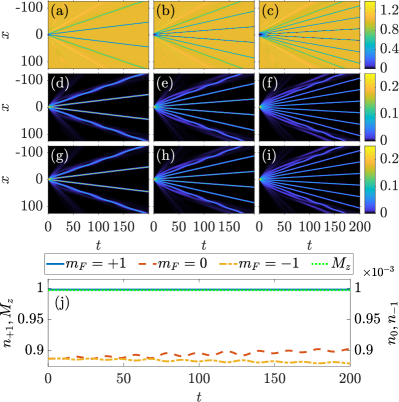
Figure 9: Spatio-temporal evolution of the density $\left|\Psi_{m_{F}}\right|^{2}$ of the (a)-(c) $m_{F}={+1}$, (d)-(f) $m_{F}={0}$, and (g)-(i) $m_{F}={-1}$ component respectively for varying $a_{+1}$. From left to right $a_{+1}=3$, $a_{+1}=5$ and $a_{+1}=7$, allowing the generation of four [(a), (d), (g)], six [(b), (e), (h)] and eight [(c), (f), (i)] DBB solitons respectively for the homogeneous spinor setting. In all cases, (a)-(c) illustrate the formation of dark solitons in the $m_{F}={+1}$ component and (d)-(f) [(g)-(i)] depict the formation of bright solitons in the $m_{F}={0}$ [$m_{F}={-1}$] component of the spinor system. (j) Evolution of the population, $n_{m{{}_{F}}}$, of each hyperfine component, and of the total magnetization, $M_{z}(t)$ for $a_{+1}=5$. Notice that $n_{0}$ and $n_{-1}$ are three orders of magnitude smaller than $n_{+1}$ which is why a second axis is introduced.

Up to now, the controlled formation of multiple soliton complexes of the DB type in two- and three-component BECs has been established. In what follows we turn our attention to the spinor $F=1$ BEC Bersano et al. (2018). In this way, we will be able to address the fate of the generated DDB and DBB soliton arrays when spin degrees of freedom are taken into account. Recall, that the evolution of this system is dictated by Eqs. (LABEL:eq:spinor_hamiltonian_a)-(LABEL:eq:spinor_hamiltonian_b). In order to induce the dynamics we will utilize once more the counterflow processes introduced in Sec. II.2.

As usual, we start our analysis by considering the homogeneous system. As in the previous section, for a DDB generation process the initial ansatz used for the $m_{F}=+1,0$ [$m_{F}=-1$] components is given by Eq. (5) [Eq. (10)]. Accordingly, to dynamically produce DBB soliton arrays the corresponding initial conditions are provided by Eq. (10) [Eq. (5)] for the $m_{F}=0,-1$ [$m_{F}=+1$] hyperfine components. Figures 9(a)-9(j) and Figs. 10(a)-10(j) summarize our numerical findings. In particular, Figs. 9(a)-(i) illustrate the evolution of the density, $\left|\Psi_{m_{F}}\right|^{2}$, of all three $m_{F}=+1,0,-1$ components. The controlled generation of four, six and eight DBB soliton arrays can be readily seen as $a_{+1}$ is increased from $a_{+1}=3$ to $a_{+1}=7$ [see Figs. 9(a), (d), (g), Figs. 9(b), (e), (h) and Figs. 9(c), (f), (i), respectively]. Comparing the dynamical evolution of the spinor system to the one observed in the corresponding three-component setting [see Figs. 6(a)-6(f)] it becomes apparent that the inclusion of the spin interaction has a minuscule effect on both the nucleation and the long time evolution of the DBB states. To appreciate the latter, in Fig. 9(j) we monitor the temporal evolution of the population, i.e. $n_{m_{F}}(t)=\frac{1}{N}\int|\Psi_{m_{F}}\left(x,t\right)|^{2}\text{d}x$, of each hyperfine component, as well as the total magnetization $M_{z}(t)=\int\left(|\Psi_{+1}\left(x,t\right)|^{2}-|\Psi_{-1}\left(x,t\right)|^{2}\right)\text{d}x$ of the spinor system for $a_{+1}=5$ (see also Sec. II.1). Note that $n_{0}(t)$, $n_{-1}(t)$ are multiplied by a factor of $10^{3}$ in order to be visible, and that the same picture holds equally for all the distinct variations of $a_{+1}$ presented in Fig. 9. As it can be deduced, oscillations of $n_{+1}(t)$, $n_{0}(t)$ and $n_{-1}(t)$ occur during the evolution. Recall now, that a spinor condensate is subject to the so-called spin relaxation process. The latter, allows for collisions of two $m_{F}=0$ atoms that can in turn produce a pair of particles in the $m_{F}=+1$ and $m_{F}=-1$ component and vice versa Chang et al. (2005). It is this continuous exchange of particles that leads to the oscillatory trajectories observed for the bright soliton constituents of the resulting DBB arrays. Notice that $n_{+1}(t)$ is significantly larger when compared to $n_{0,-1}(t)\sim 10^{-3}$ and due to the rescaling used appears almost constant ($n_{+1}(t)\approx 1$) during evolution. However, we must stress that also not discernible oscillations of the population of this hyperfine component are present and are similar to the ones observed for the $n_{-1}(t)$ component. Therefore $M_{z}(t)$ remains constant during the evolution while being of order unity.

Contrary to the DBB nucleation process investigated above, for a DDB realization the spin-mixing dynamics plays a crucial role. As in the previous scenario, Figs. 10(a)-10(i) show the spatio-temporal evolution of the densities, $\left|\Psi_{m_{F}}\right|^{2}$, of all three $m_{F}$ components. Also here, by manipulating $a_{+1}=a_{0}=a$ we were able to controllably generate arrays of DDB solitons in this homogeneous spinor setting. From left to right in this figure, six, eight and twelve solitons are formed, corresponding to $a=3$, $a=5$ and $a=7$ respectively. In particular, Figs. 10(a)-(c) [Figs. 10(d)-(f)] depict the dark solitons formed in the $m_{F}=+1$ [$m_{F}=0$] component. Additionally, Figs. 10(g)-(i) illustrate the bright states formed in the respective $m_{F}=-1$ component. Strikingly enough, as it is observed in all of the aforementioned contour plots, as time evolves, the background density gradually changes (notice the change in the color gradient). This result, as we will show later on, is attributed to the spin-mixing dynamics that significantly alters the evolution of the DDB soliton arrays formed.

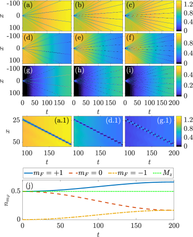
Figure 10: Same as in Fig. 9 but showcasing the generation of DDB solitons. In all cases, (a)-(c) [(d)-(f)] illustrate the formation of dark solitons in the $m_{F}={+1,0}$ components and (g)-(i) illustrate the formation of bright solitons in the $m_{F}={-1}$ component of the spinor system. ($a_{1}$), ($d_{1}$), ($g_{1}$) Trajectory of the closest to the origin right moving originally formed DDB soliton shown in (a), (d), (g) transitioning during evolution into beating dark states. (j) Evolution of the population, $n_{m_{F}}$, of each hyperfine component, as well as of the total magnetization, $M_{z}(t)$, for $a_{+1}=a_{0}=5$.

To shed light on the observed dynamics, below let us focus our attention on Figs. 10(a), 10(d) and 10(g) for $a=3$. Here, also a zoom is provided in Figs. 10($a.1$), 10($d.1$) and 10($g.1$) to elucidate our analysis. In the latter figures the closest to the origin DDB pair is monitored. As time evolves the background density of the $m_{F}=+1$ component increases which suggests that transfer of particles from the lower hyperfine components takes place. The latter can indeed be confirmed by inspecting the evolution of the $m_{F}=0$ component. Evidently, the background density of this component gradually decreases. The corresponding density of the $m_{F}=-1$ component is also seen to increase. Monitoring the evolution of the respective populations, $n_{m_{F}}(t)$, shown in Fig. 10(j), delineates the above trend. Indeed, at $t=0$ $n_{+1}(0)=n_{0}(0)=0.5$ while $n_{-1}(0)\sim 10^{-3}$. However, during evolution $n_{+1}(t)$ increases reaching the value of $n_{+1}(t=200)\approx 0.66$. Accordingly, $n_{0}(t)$ decreases drastically during propagation acquiring a similar value with $n_{-1}(t)$ at later evolution times, i.e. $n_{0}(t=200)\approx n_{-1}(t=200)\approx 0.16$. Note also, that the total magnetization of the system is preserved with $M_{z}(t)=0.5$ throughout the evolution. Returning now to the relevant densities, since the background density of the $m_{F}=0$ component decreases, the dark states formed in this component begin to deform. At later times ($t>150$) the solitonic states developed in this hyperfine component have both a dark and a bright component [see Fig. 10($d.1$)]. Similarly, at early times the $m_{F}=-1$ component hosts bright solitons. Since the number of particles, in this case increases, a finite background slowly appears Li et al. (2005); Kurosaki and Wadati (2007). As such, also the bright solitons of this component begin to deform. The latter deformation leads in turn to the formation of solitonic structures that again have both a bright and a dark part, involving a breathing between the two and are formed also faster in this $m_{F}=-1$ when compared to $m_{F}=0$ one [see Fig. 10($g.1$)]. The same deformation occurs also in the $m_{F}=+1$ component but at propagation times even larger than the ones depicted in Fig. 10(a). Indeed, by inspecting the evolution of the closest to the origin dark soliton of the originally formed DDB state shown in Fig. 10($a.1$), the dark soliton is also deformed in this case, yet the beating pattern of panel ($g.1$) [and even that of ($d.1$)] is not as straightforwardly discernible. Nevertheless, close inspection indicates that the evolved states in all three $m_{F}$ components bear similar characteristics to the so-called beating dark solitons that were experimentally observed in two-component systems Yan et al. (2012). As such, these states can be thought of as the generalization of the beating dark solitons in spinor BECs.

Before proceeding to the harmonically confined spinor BEC system, a final comment is of relevance here. Investigating the current setting, we also considered different initializations in which the symmetric, with respect to the $m_{F}=0$, hyperfine states have the same initial conditions. In this way we were able to generate symmetric variants of the DDB and DBB states discussed above. Namely, DBD and BDB soliton arrays. In these cases, our simulations indicate that the resulting states show all features found in the three-component setting. Although the spin interaction is present, the conversion of particles from one component to another is six orders of magnitude smaller than the total number of particles. As such the spin interaction is negligible. For these systems, also the total magnetization is zero, in contrast to the finite one observed for the asymmetric, in the above sense, DDB and DBB soliton arrays addressed herein. In that light, it appears as if the drastic effect of the spin-interaction contribution in the previous realization is able to excite the beating dark soliton generalizations. On the other hand, following the approach of Yan et al. (2012) in the three-component Manakov case, it is also possible to excite beating solitons in the latter (spin-independent) case. However, a more systematic theoretical analysis of the beating states is deferred for a separated work.

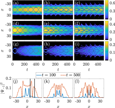
Figure 11: Spatio-temporal evolution of the densities $\left|\Psi_{m_{F}}\right|^{2}$ of the (a)-(c) $m_{F}={+1}$, (d)-(f) $m_{F}={0}$ and (g)-(i) $m_{F}={-1}$ components upon varying the width, $w$, of the double-well barrier. From left to right $w^{2}=1$, $w^{2}=5$ and $w^{2}=10$, allowing the generation of two [(a), (d), (g)], four [(b), (e), (h)] and six [(c), (f), (i)] DDB solitons respectively in the spinor system. In all cases, (a)-(c) [(d)-(f)] illustrate the formation of dark solitons in the $m_{F}={+1}$ [$m_{F}={0}$] component and (g)-(i) the generated bright solitons, transitioning into beating dark states, in the $m_{F}={-1}$ component. (j)-(l) Vertical cuts of $\left|\Psi_{-1}\right|^{2}$ for the three distinct values of $w$ (see legend). In (j) solid rectangle indicates a beating dark soliton.

In the trapped scenario we exclusively present our findings for a DDB generation process. This is due to the fact that only this nucleation process entails new features stemming from the spin-mixing dynamics. The initial state preparation used herein is the one described in the confined three-component setting (see Sec. III.2). Once more, by properly adjusting the initial width, $w$, of the double-well potential [see Eq. (11)] the controlled formation of multiple DDB soliton complexes is achieved in this harmonically trapped spinor system. From top to bottom Figs. 11(a)-(i) show the evolution of $\left|\Psi_{m_{F}}\right|^{2}$ (with $m_{F}=+1,0,-1$). As $w^{2}$ is increased from $w^{2}=1$ to $w^{2}=10$ two, four and six such solitons are formed [e.g. see Figs. 11(a)-(c)]. Dark solitons emerge in the $m_{F}=+1,0$ components [see Figs. 11(a)-(c), 11(d)-(f)] while bright states are generated in the $m_{F}=-1$ component [see Figs. 11(g)-(i)]. However, as in the homogeneous scenario, soon after their formation all states formed and also in all hyperfine components begin to deform. This deformation occurs faster in the less populated $m_{F}=-1$ component and later on in the other two hyperfine states. This phenomenon is yet again attributed to the spin-mixing dynamics that allows for particle exchange between the components. Focusing on Figs. 11(a), (d), (g), the background densities of both the $m_{F}=\pm 1$ components increase while the density of the $m_{F}=0$ one decreases. This exchange in population leads in turn during evolution to a transition of the soliton states in each component into states that bear both a dark and a bright part. Thus, in line with our findings in the homogeneous case, beating dark solitons are progressively formed in all three hyperfine components. Since these beating structures are more pronounced in the $m_{F}=-1$ component, in Fig. 11(j) profile snapshots of the density of this component are illustrated. In particular, $|\Psi_{-1}|^{2}$ is depicted for two different time instants, namely $t=100$ and $t=500$, during the evolution and for $w^{2}=1$. At initial times the two bright solitons originally formed in this component are now on top of a still small, yet finite background. Namely, they are already deformed into states that are reminiscent of the so-called antidark solitons Danaila et al. (2016); Kevrekidis et al. (2004); Katsimiga et al. (2017c). At larger evolution times, instead of the aforementioned antidark solitons, two beating dark states are seen to propagate. One of them is indicated in Fig. 11(j) by a black rectangle. Notice that this beating state has a density dip followed be a density hump.

The above-discussed dynamical evolution of the spinor system holds equally for all the different variations illustrated in Figs. 11(a)-(i). However, the deformation of the DDB states is found to be delayed as $w^{2}$ is increased. The latter result can be deduced by comparing at earlier evolution times the density profile shown in Fig. 11(l) to the relevant ones illustrated in Figs. 11(j), (k). Additionally, and also in all cases depicted in Figs. 11(a)-(i), the initially formed DDB structures that evolve later on into beating dark solitons are seen to oscillate and interact within the parabolic trap. However, while coherent oscillations are observed in Figs. 11(a), (d), (g), incoherent ones occur when the number of states is increased (i.e. for increasing $w^{2}$). In these latter cases, as shown in Figs. 11(b), (e), (h), several collision events between the outer and the inner beating states take place. Despite the much more involved dynamical evolution of the spinor system in such cases, these beating states remain robust for all the evolution examples that we have checked. Furthermore, we also explored the dynamical evolution of the spinorial BEC system for different values of the chemical potential, $\mu$. Similarly to the aforementioned $w$ variation, a controlled formation of larger DDB arrays as $\mu$ increases can be once more verified. The resulting states in increasing order, in terms of $\mu$, are presented in Figs. 12(a)-(i) for fixed $w^{2}=5$. Notice that since $w^{2}=5$ Figs. 12(a)-(c) are respectively identical to Figs. 11(b), 11(e) and 11(h). However, increasing $\mu$ increases the system’s size. As such, arrays consisting of a larger number of DDB solitons are formed. Indeed, six and eight DDB states are generated for $\mu=3$ and $\mu=5$ respectively. Importantly here, it is found that the presence of the spin interaction has a more dramatic effect on the resulting states when compared to the previous variation. Namely, the originally formed DDB structures transition into beating dark ones much faster when compared to the $w$ variation. A case example can be seen in Fig. 12(g), corresponding to $\mu=5$, where the dark solitons of the $m_{F}=+1$ component evolve into beating ones already at $t=150$. Even for the largest $w^{2}=10$ value considered above, such a transition occurs for this hyperfine component at evolution times $t\approx 300$ [see Fig. 11(c)]. To appreciate the effect of the spin interaction, we monitor during evolution the population, $n_{m_{F}}(t)$ ($m_{F}=+1,0,-1$), of each hyperfine component and for all the different values of $\mu$ considered herein. In particular, from left to right Figs. 12(j)-(l) illustrate $n_{+1}(t)$, $n_{0}(t)$ and $n_{-1}(t)$ respectively. Notice that the population of each hyperfine component is affected more, the larger the value of $\mu$ is. Evidently, the monotonic increase ($n_{\pm 1}(t)$) or decrease ($n_{0}(t)$) for $\mu=1$ turns into damping oscillations as $\mu$ increases. Such a coherent spin-mixing dynamics is in line with earlier predictions in spinor $F=1$ BECs Pu et al. (1999); Chang et al. (2005). Finally, we verified that the total magnetization $M_{z}(t)$ remains constant during evolution acquiring a slightly smaller value as $\mu$ is increased [see the inset in Fig. 12(l)].

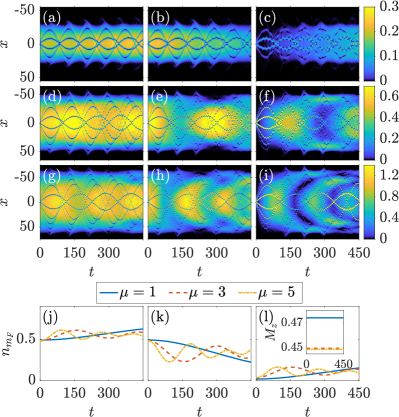
Figure 12: Same as Fig. 11 but upon varying the chemical potential $\mu$. From top to bottom $\mu=1$, $\mu=3$ and $\mu=5$, allowing the generation of four [(a)-(c)], six [(d)-(f)] and eight [(g)-(i)] DDB solitons respectively. In all cases, (a), (d), (g) [(b), (e), (h)] illustrate the formation of dark solitons in the $m_{F}={+1}$ [$m_{F}={0}$] component and (c), (f), (i) the generated bright solitons in the $m_{F}={-1}$ component of the spinor system. Notice that the colormap has a $2.5:2:1$ ratio between the columns. (j)-(l) Evolution of the normalized number of particles, $n_{m_{F}}(t)$, for each value of $\mu$. The inset in (l) shows the total magnetization, $M_{z}(t)$, for each value of $\mu$.

IV Conclusions and Future perspectives

In this work the controlled creation of multiple soliton complexes of the DB type that appear in one-dimensional two-component, three-component and spinor BECs has been investigated. Direct numerical simulations of each system’s dynamical evolution have been performed both in the absence and in the presence of a parabolic trap. In all models considered herein, the nucleation process is based on the so-called matter wave interference of separated condensates being utilized to study multi-component systems. In this sense, this work offers a generalization of earlier findings in single-component setups to the much more involved multi-component ones, enabling the identification of dark-bright solitons in two-component and dark-dark-bright and dark-bright-bright solitons in three-component (and spinorial) gases. To achieve control over each system’s dynamical evolution different parametric variations have been considered.

In particular, for the homogeneous systems addressed in this effort, inverse rectangular pulses were employed for the components featuring interference, and Gaussian ones for the remaining participating components. Destructive interference of the two sides of the former pulse leads to the nucleation of an array of dark soltions. Additionally, the dispersion of the Gaussian pulse and its subsequent confinement in the effective potential created by each of the nucleated dark solitons results in the formation of bright solitons that are subsequently trapped and waveguided by their corresponding dark counterparts. It is found that manipulating the width of the IRP is sufficient to ensure the desired nucleation of multiple soliton compounds of the DB type. This way, arrays of DB, and DDB and DBB solitons are dynamically produced in the two-component and spinor cases, respectively. Moreover, for the two-component system it is showcased that each of the generated DB solitons follows the analytical expressions stemming from the integrable theory of the Manakov system. The same holds true also for the DBB and DDB states nucleated in the three component system. In the latter, generalized expressions that connect the soliton parameters are extracted and used to appreciate modifications of the soliton characteristics under different parametric variations. While the same overall dynamical evolution is observed for the two- and three-component systems, a significantly different picture can be drawn for the spinorial case. Strikingly, and for a DDB nucleation process, it is found that during evolution the originally formed DDB soliton arrays begin to deform due to the spin-mixing dynamics. The latter allows for exchange of particles between the hyperfine components. The aforementioned deformation leads in turn to the gradual formation of arrays of beating dark states. The latter, once formed, are seen to robustly propagate for large evolution times. The existence of beating dark states in spinor systems has not, to the best of our knowledge, been reported previously and it is an interesting topic for further exploration.

For the harmonically trapped scenarios our numerical findings suggest similar characteristics as in the homogeneous cases in terms of the nucleation process, although naturally the dynamics is rendered more complex due to the confinement and the induced interactions between the produced solitary waves. In all cases it is found that by adjusting the width of the rectangular pulse or the chemical potential of the participating components, the desirable number of DB, DDB and DBB soliton complexes can be generated. This provides a sense of dynamical control and design of desired configurations in our system. The number of the resulting coherent structures is found to increase upon increasing each of the above parameters. In the trapped case, the resulting multi-soliton arrays, irrespectively of their type, are found to oscillate and interact within the parabolic trap being robust for large evolution times. Contrary to the above findings, for the spinorial BEC system a departure of the initially formed DDB states to the beating dark ones is showcased. Here, coherent spin-mixing dynamics is observed when monitoring the population of each hyperfine component. Damping oscillations of the latter occur, that are found to be enhanced upon increasing, for example, the chemical potential of each component. Additionally, and also in comparison to the homogeneous case, the beating dark states are formed faster in the trapped setting. This formation is further enhanced the larger the chemical potential is. It is found that the beating dark solitons persist while oscillating and interacting with one another. The existence of these spinorial beating states can be tested in current state-of-the art experiments Bersano et al. (2018), and it is clearly a direction of interest in its own right for future studies. More specifically, it would be particularly interesting to generalize the findings associated with the two-component beating dark solitons Yan et al. (2012) to the spinor case and study in a detailed manner the formation and interactions of the spinor beating dark states identified herein.

Yet, another interesting perspective would be to compare and contrast the numerically identified DDB and DBB states of the three-component system to the analytical expressions that are available, at least for the integrable version of this model Biondini et al. (2016). More specifically, one could generalize the criteria of the single component IRP scenario obtained in the earlier works of Zakharov and Shabat (1973) to the formation of both DB and also DDB or DBB solitons from similar initial data in the multi-component case and compare these predictions against the corresponding numerical computations. Then, one could depart from the above Manakov limit and also study the fate of these structures in non-integrable systems Katsimiga et al. (2018a), including the spinor one. The breaking of integrability would allow in turn for effects such as the miscibility/immiscibility of the involved components to come into play Kiehn et al. (2019). The interplay of the resulting density variations with the potential persistence of the solitary wave structures is an interesting topic for future study. Also in the same context it would be interesting to systematically examine interactions between multiple DDB and DBB states. The role of other effects such as the potential Rabi coupling between the components could also be of interest in its own right Pitaevskii and Stringari (2016, 2016).

Lastly, as has been discussed in relevant reviews such as Kevrekidis and Frantzeskakis (2016), many of these ideas, such as the DB solitons (generalizing to vortex-bright ones), the beating dark solitons, etc., naturally generalize to corresponding higher-dimensional states. Examining the potential for such states as a result of interference or possibly other methods more concretely associated with higher dimensions such as the transverse instability would be of particular interest in its own right.

References

- Anderson et al. (1995) M. H. Anderson, J. R. Ensher, M. R. Matthews, C. E. Wieman, and E. A. Cornell, Science 269, 198 (1995).
- Davis et al. (1995) K. B. Davis, M. O. Mewes, M. R. Andrews, N. J. van Druten, D. S. Durfee, D. M. Kurn, and W. Ketterle, Phys. Rev. Lett. 75, 3969 (1995).
- Frantzeskakis (2010) D. J. Frantzeskakis, J. Phys. A 43, 213001 (2010).
- Abdullaev et al. (2005) F. Abdullaev, A. Gammal, A. Kamchatnov, and L. Tomio, Int. J. Mod. Phys. B 19, 3415 (2005).
- Zakharov and Shabat (1972) V. E. Zakharov and A. B. Shabat, Sov. J. Exp. Theor. Phys. 34, 62 (1972).
- Zakharov and Shabat (1973) V. E. Zakharov and A. B. Shabat, Sov. J. Exp. Theor. Phys. 37, 823 (1973).
- Becker et al. (2008) C. Becker, S. Stellmer, P. Soltan-Panahi, S. Dörscher, M. Baumert, E.-M. Richter, J. Kronjäger, K. Bongs, and K. Sengstock, Nat. Phys. 4, 496 (2008).
- Middelkamp et al. (2011) S. Middelkamp, J. Chang, C. Hamner, R. Carretero-González, P. Kevrekidis, V. Achilleos, D. Frantzeskakis, P. Schmelcher, and P. Engels, Phys. Lett. A 375, 642 (2011).
- Hamner et al. (2011) C. Hamner, J. J. Chang, P. Engels, and M. A. Hoefer, Phys. Rev. Lett. 106, 065302 (2011).
- Yan et al. (2011) D. Yan, J. J. Chang, C. Hamner, P. G. Kevrekidis, P. Engels, V. Achilleos, D. J. Frantzeskakis, R. Carretero-González, and P. Schmelcher, Phys. Rev. A 84, 053630 (2011).
- Hoefer et al. (2011) M. A. Hoefer, J. J. Chang, C. Hamner, and P. Engels, Phys. Rev. A 84, 041605 (2011).
- Yan et al. (2012) D. Yan, J. J. Chang, C. Hamner, M. Hoefer, P. G. Kevrekidis, P. Engels, V. Achilleos, D. J. Frantzeskakis, and J. Cuevas, J. Phys. B: At. Mol. Opt. Phys. 45, 115301 (2012).
- Brazhnyi and Pérez-García (2011) V. A. Brazhnyi and V. M. Pérez-García, Chaos, Solitons & Fractals 44, 381 (2011).
- Yin et al. (2011) C. Yin, N. G. Berloff, V. M. Pérez-García, D. Novoa, A. V. Carpentier, and H. Michinel, Phys. Rev. A 83, 051605 (2011).
- Achilleos et al. (2011) V. Achilleos, P. G. Kevrekidis, V. M. Rothos, and D. J. Frantzeskakis, Phys. Rev. A 84, 053626 (2011).
- Álvarez et al. (2013) A. Álvarez, J. Cuevas, F. R. Romero, C. Hamner, J. J. Chang, P. Engels, P. G. Kevrekidis, and D. J. Frantzeskakis, J. Phys. B: At. Mol. Opt. Phys. 46, 065302 (2013).
- Yan et al. (2015) D. Yan, F. Tsitoura, P. G. Kevrekidis, and D. J. Frantzeskakis, Phys. Rev. A 91, 023619 (2015).
- Karamatskos et al. (2015) E. T. Karamatskos, J. Stockhofe, P. G. Kevrekidis, and P. Schmelcher, Phys. Rev. A 91, 043637 (2015).
- Katsimiga et al. (2017a) G. C. Katsimiga, J. Stockhofe, P. G. Kevrekidis, and P. Schmelcher, Phys. Rev. A 95, 013621 (2017a).
- Katsimiga et al. (2017b) G. C. Katsimiga, J. Stockhofe, P. G. Kevrekidis, and P. Schmelcher, Appl. Sci. 7, 388 (2017b).
- Katsimiga et al. (2018a) G. C. Katsimiga, P. G. Kevrekidis, B. Prinari, G. Biondini, and P. Schmelcher, Phys. Rev. A 97, 043623 (2018a).
- Kevrekidis and Frantzeskakis (2016) P. Kevrekidis and D. Frantzeskakis, Rev. Phys. 1, 140 (2016).
- Trillo et al. (1988) S. Trillo, S. Wabnitz, E. M. Wright, and G. I. Stegeman, Opt. Lett. 13, 871 (1988).
- Christodoulides (1988) D. N. Christodoulides, Phys. Lett. A 132, 451 (1988).
- Ostrovskaya and Kivshar (1998) E. A. Ostrovskaya and Y. S. Kivshar, Opt. Lett. 23, 1268 (1998).
- Afanasyev et al. (1989) V. V. Afanasyev, Y. S. Kivshar, V. V. Konotop, and V. N. Serkin, Opt. Lett., OL 14, 805 (1989).
- Kivshar and Turitsyn (1993) Y. S. Kivshar and S. K. Turitsyn, Opt. Lett. 18, 337 (1993).
- Christodoulides et al. (1996) D. N. Christodoulides, S. R. Singh, M. I. Carvalho, and M. Segev, Appl. Phys. Lett. 68, 1763 (1996).
- Buryak et al. (1996) A. V. Buryak, Y. S. Kivshar, and D. F. Parker, Phys. Lett. A 215, 57 (1996).
- Sheppard and Kivshar (1997) A. P. Sheppard and Y. S. Kivshar, Phys. Rev. E 55, 4773 (1997).
- Chen et al. (1997) Z. Chen, M. Segev, T. H. Coskun, D. N. Christodoulides, and Y. S. Kivshar, J. Opt. Soc. Am. B, JOSAB 14, 3066 (1997).
- Kivshar and Luther-Davies (1998) Y. S. Kivshar and B. Luther-Davies, Phys. Rep. 298, 81 (1998).
- Ostrovskaya et al. (1999) E. A. Ostrovskaya, Y. S. Kivshar, Z. Chen, and M. Segev, Opt. Lett., OL 24, 327 (1999).
- Park and Shin (2000) Q.-H. Park and H. J. Shin, Phys. Rev. E 61, 3093 (2000).
- Stamper-Kurn and Ketterle (2001) D. M. Stamper-Kurn and W. Ketterle, in Coherent Atomic Matter Waves, Les Houches - Ecole d’Ete de Physique Theorique, edited by R. Kaiser, C. Westbrook, and F. David (Springer Berlin Heidelberg, 2001) pp. 139–217.
- Chang et al. (2004) M.-S. Chang, C. D. Hamley, M. D. Barrett, J. A. Sauer, K. M. Fortier, W. Zhang, L. You, and M. S. Chapman, Phys. Rev. Lett. 92, 140403 (2004).
- Chang et al. (2005) M.-S. Chang, Q. Qin, W. Zhang, L. You, and M. S. Chapman, Nat. Phys. 1, 111 (2005).
- Kawaguchi and Ueda (2012) Y. Kawaguchi and M. Ueda, Physics Reports Spinor Bose–Einstein Condensates, 520, 253 (2012).
- Stamper-Kurn and Ueda (2013) D. M. Stamper-Kurn and M. Ueda, Rev. Mod. Phys. 85, 1191 (2013).
- Ohmi and Machida (1998) T. Ohmi and K. Machida, J. Phys. Soc. Jpn. 67, 1822 (1998).
- Tsuchida and Wadati (1998) T. Tsuchida and M. Wadati, J. Phys. Soc. Jpn. 67, 1175 (1998).
- Ieda et al. (2004a) J. Ieda, T. Miyakawa, and M. Wadati, Phys. Rev. Lett. 93, 194102 (2004a).
- Ieda et al. (2004b) J. Ieda, T. Miyakawa, and M. Wadati, J. Phys. Soc. Jpn. 73, 2996 (2004b).
- Ieda (2005) J. Ieda, Study of Matter-Wave Solitons in Spinor Bose-Einstein Condensates, PhD Thesis, Tokyo University (2005).
- Li et al. (2005) L. Li, Z. Li, B. A. Malomed, D. Mihalache, and W. M. Liu, Phys. Rev. A 72, 033611 (2005).
- Wadati and Tsuchida (2005) M. Wadati and N. Tsuchida, J. Phys. Soc. Jpn. 75, 014301 (2005).
- Ieda et al. (2006) J. Ieda, T. Miyakawa, and M. Wadati, Laser Phys. 16, 678 (2006).
- Uchiyama et al. (2006) M. Uchiyama, J. Ieda, and M. Wadati, J. Phys. Soc. Jpn. 75, 064002 (2006).
- Ieda et al. (2007) J. Ieda, M. Uchiyama, and M. Wadati, J. Math. Phys. 48, 013507 (2007).
- Zhang et al. (2007) W. Zhang, O. E. Müstecaplıoğlu, and L. You, Phys. Rev. A 75, 043601 (2007).
- Kurosaki and Wadati (2007) T. Kurosaki and M. Wadati, J. Phys. Soc. Jpn. 76, 084002 (2007).
- Dabrowska-Wüster et al. (2007) B. J. Dabrowska-Wüster, E. A. Ostrovskaya, T. J. Alexander, and Y. S. Kivshar, Phys. Rev. A 75, 023617 (2007).
- Nistazakis et al. (2008) H. E. Nistazakis, D. J. Frantzeskakis, P. G. Kevrekidis, B. A. Malomed, and R. Carretero-González, Phys. Rev. A 77, 033612 (2008).
- Xiong and Gong (2010) B. Xiong and J. Gong, Phys. Rev. A 81, 033618 (2010).
- Bersano et al. (2018) T. M. Bersano, V. Gokhroo, M. A. Khamehchi, J. D’Ambroise, D. J. Frantzeskakis, P. Engels, and P. G. Kevrekidis, Phys. Rev. Lett. 120, 063202 (2018).
- Katsimiga et al. (2018b) G. C. Katsimiga, S. I. Mistakidis, G. M. Koutentakis, P. G. Kevrekidis, and P. Schmelcher, Phys. Rev. A 98, 013632 (2018b).
- Brazhnyi and Kamchatnov (2003) V. A. Brazhnyi and A. M. Kamchatnov, Phys. Rev. A 68, 043614 (2003).
- Dutton et al. (2001) Z. Dutton, M. Budde, C. Slowe, and L. V. Hau, Science 293, 663 (2001).
- Engels and Atherton (2007) P. Engels and C. Atherton, Phys. Rev. Lett. 99, 160405 (2007).
- Shomroni et al. (2009) I. Shomroni, E. Lahoud, S. Levy, and J. Steinhauer, Nat. Phys. 5, 193 (2009).
- Burger et al. (1999) S. Burger, K. Bongs, S. Dettmer, W. Ertmer, K. Sengstock, A. Sanpera, G. V. Shlyapnikov, and M. Lewenstein, Phys. Rev. Lett. 83, 5198 (1999).
- Denschlag et al. (2000) J. Denschlag, J. E. Simsarian, D. L. Feder, C. W. Clark, L. A. Collins, J. Cubizolles, L. Deng, E. W. Hagley, K. Helmerson, W. P. Reinhardt, S. L. Rolston, B. I. Schneider, and W. D. Phillips, Science 287, 97 (2000).
- Anderson et al. (2001) B. P. Anderson, P. C. Haljan, C. A. Regal, D. L. Feder, L. A. Collins, C. W. Clark, and E. A. Cornell, Phys. Rev. Lett. 86, 2926 (2001).
- Weller et al. (2008) A. Weller, J. P. Ronzheimer, C. Gross, J. Esteve, M. K. Oberthaler, D. J. Frantzeskakis, G. Theocharis, and P. G. Kevrekidis, Phys. Rev. Lett. 101, 130401 (2008).
- Hoefer et al. (2009) M. A. Hoefer, P. Engels, and J. J. Chang, Physica D: Nonlinear Phenomena 238, 1311 (2009).
- Scherer et al. (2007a) D. R. Scherer, C. N. Weiler, T. W. Neely, and B. P. Anderson, Phys. Rev. Lett. 98, 110402 (2007a).
- Reinhardt and Clark (1997) W. P. Reinhardt and C. W. Clark, J. Phys. B: At. Mol. Opt. Phys. 30, 785 (1997).
- Scott et al. (1998) T. F. Scott, R. J. Ballagh, and K. Burnett, J. Phys. B: At. Mol. Opt. Phys. 31, 329 (1998).
- Theocharis et al. (2010) G. Theocharis, A. Weller, J. P. Ronzheimer, C. Gross, M. K. Oberthaler, P. G. Kevrekidis, and D. J. Frantzeskakis, Phys. Rev. A 81, 063604 (2010).
- Öhberg and Santos (2001) P. Öhberg and L. Santos, Phys. Rev. Lett. 86, 2918 (2001).
- Pu et al. (1999) H. Pu, C. K. Law, S. Raghavan, J. H. Eberly, and N. P. Bigelow, Phys. Rev. A 60, 1463 (1999).
- Ho (1998) T.-L. Ho, Phys. Rev. Lett. 81, 742 (1998).
- Klausen et al. (2001) N. N. Klausen, J. L. Bohn, and C. H. Greene, Phys. Rev. A 64, 053602 (2001).
- van Kempen et al. (2002) E. G. M. van Kempen, S. J. J. M. F. Kokkelmans, D. J. Heinzen, and B. J. Verhaar, Phys. Rev. Lett. 88, 093201 (2002).
- Manakov (1973) S. V. Manakov, Zh. Eksp. Teor. Fiz. 65, 505 (1973).
- Biondini et al. (2016) G. Biondini, D. K. Kraus, and B. Prinari, Comm. Math. Phys. 348, 475 (2016).
- Kevrekidis et al. (2015) P. G. Kevrekidis, D. J. Frantzeskakis, and R. Carretero-González, The defocusing nonlinear Schrödinger equation: from dark solitons to vortices and vortex rings (SIAM, 2015).
- Gross (1961) E. P. Gross, Nuovo Cim 20, 454 (1961).
- Pitaevskii (1961) L. P. Pitaevskii, Sov. J. Exp. Theor. Phys. 13, 451 (1961).
- Espínola-Rocha and Kevrekidis (2009) J. A. Espínola-Rocha and P. Kevrekidis, Math. Comput. Simul. 80, 693 (2009).
- Nikolov et al. (2004) N. I. Nikolov, D. Neshev, W. Królikowski, O. Bang, J. J. Rasmussen, and P. L. Christiansen, Opt. Lett., OL 29, 286 (2004).
- Scherer et al. (2007b) D. R. Scherer, C. N. Weiler, T. W. Neely, and B. P. Anderson, Phys. Rev. Lett. 98, 110402 (2007b).
- Pitaevskii and Stringari (2016) L. Pitaevskii and S. Stringari, Bose-Einstein condensation and superfluidity, Vol. 164 (Oxford University Press, 2016).
- Busch and Anglin (2001) T. Busch and J. R. Anglin, Phys. Rev. Lett. 87, 010401 (2001).
- Danaila et al. (2016) I. Danaila, M. A. Khamehchi, V. Gokhroo, P. Engels, and P. G. Kevrekidis, Phys. Rev. A 94, 053617 (2016).
- Kevrekidis et al. (2004) P. G. Kevrekidis, H. E. Nistazakis, D. J. Frantzeskakis, B. A. Malomed, and R. Carretero-González, EPJD: Atom., Mol., Opt. Pl. Phys. 28, 181 (2004).
- Katsimiga et al. (2017c) G. C. Katsimiga, G. M. Koutentakis, S. I. Mistakidis, P. G. Kevrekidis, and P. Schmelcher, New J. Phys. 19, 073004 (2017c).
- Kiehn et al. (2019) H. Kiehn, S. I. Mistakidis, G. Katsimiga, and P. Schmelcher, arXiv:1902.09316 (2019).