Liquid-Gas Phase Transition in Nuclei

Abstract

This review article takes stock of the progress made in understanding the phase transition in hot nuclei and highlights the coherence of observed signatures.

, ,

1 Introduction

Phase transitions are universal properties of interacting matter and traditionally they have been studied in the thermodynamic limit of macroscopic systems. A phase transition occurs when a phase becomes unstable in given thermodynamical conditions described with intensive variables like temperature, pressure … The interaction between nucleons in nuclei is similar to the interaction between molecules in a van der Waals fluid: a short-distance repulsive core and a long-distance attractive tail. It is the reason why Bertsch and Siemens [1] suggested that the nuclear interaction should lead to a liquid-gas (LG) phase transition in nuclei. This original work also suggested that if the equation of state of nuclear matter is of van der Waals type, nucleus-nucleus collision experiments may bring excited nuclei into the spinodal region of the phase diagram in which spinodal instabilities may develop exponentially and lead to the spectacular break-up of nuclei commonly called multifragmentation. Starting from this work, considerable theoretical and experimental efforts were made to yield a better understanding of possible scenarios [2]. In particular, one part of the theoretical effort was devoted to the consequences of finite size effects as far as the phase transition signatures are concerned [3, 4, 5]. With isolated finite systems like nuclei, the concept of thermodynamic limit cannot apply and extensive variables like energy and entropy are no longer additive due to the important role played by surfaces. On the experimental side, studies are performed using heavy-ion collisions at intermediate and relativistic energies and hadron-nucleus collisions at relativistic energies. Detailed studies of reaction products are obtained with powerful multidetectors [6] allowing the detection of a large amount of the many fragments and light particles produced. It also appears that further progress is linked to the knowledge of many observables which gives the possibility to study correlations inside the multifragment events and to realize very constrained simulations.

This review is exclusively focused on manifestations of the nuclear LG phase transition in hot nuclei. A variety of reviews of nuclear multifragmentation and of related dynamical and statistical models are available for a thorough description and analysis of the field [7, 8, 9, 10, 11, 12, 13, 14]. The present review is organized as follows. In sections 2, 3 and 4 we explain why and how to study a phase transition in hot nuclei. Section 5 illustrates the liquidlike behaviour of nuclei in their ground states or at low excitation energies and the experimental evidence that at very high excitation energies they behave like a gas. Signatures of a first-order phase transition in hot nuclei are discussed in section 6; we present the wide range of predicted behaviours and their experimental observations, before concluding with coherency of the different signals.

2 Why study a phase transition in hot nuclei?

Before presenting the phases of nuclear matter including the effects of different proton and neutron concentrations and the influence of surface and Coulomb effects when going from infinite matter to nuclei, we want to address some general comments related to thermodynamics of nuclei. We all learned that phase transitions exist only in large systems, strictly in the thermodynamic limit. However multifragmentation has long been known to be the dominant decay mode of a nucleus with $A$ nucleons at excitation energy between around $3A$ and $10A$ MeV. From this observation it became evident that concepts like entropy and phase transitions apply to such very small many-body systems typically composed of a few hundred of nucleons. Therefore an extension of conventional macroscopic and homogeneous thermodynamics to such finite systems was needed. A few words now about the concept of temperature, which was largely and successfully used at low excitation energies. At high excitation energies, to use it, one has to admit that nuclei have enough time to thermalize during collisions. From the theoretical side it was shown that energy relaxation can be totaly fulfilled depending on bombarding energies [15, 16, 17, 18] and experimental results have confirmed these expectations [19, 20]. Another more conceptual point which is of relevance to the nuclear decay problem is concerned with the ergodic hypothesis which is used in connection with single systems. The essential idea behind the ergodic hypothesis is that a system in equilibrium evolves through a representative set of all accessible microstates over a time interval associated with a measurement. For ergodic systems, a theoretical treatment of equilibrium can be constructed either in terms of the properties of a single system measured over an infinite time or, more conveniently, in terms of properties of a pseudo/fictive ensemble of constrained systems which provides a representative sample of all attainable configurations. This last possibility is relevant for studying the phase transition of nuclei even though the ergodic hypothesis does not apply in this case. Indeed the chaotic character of collisions involved to produce hot nuclei favors a large covering of statistical partitions when an homogeneous event sample is studied. This discussion will be developed and deepened in the next section.

2.1 Nuclear matter: the liquid-gas phase transition

Nuclear physics is a field that interconnects very much to adjacent fields such as elementary particle physics (at the higher energy end) or astrophysics. We will concentrate on the nuclear region below 30 MeV per nucleon excitation energy (equivalently $\thicksim$ 25 MeV temperature) and below density $\rho$ equal to 2-3 times the normal nuclear density $\rho_{0}$, which is deduced from the maximum of saturation density of finite nuclei and estimated as 0.155 $\pm$0.005 nucleons fm^-3 [21]. This represents only a rather small portion of the nuclear matter phase diagram, as predicted theoretically and displayed in Fig. 1, if we note that on the figure both axes are shown in logarithmic scale.

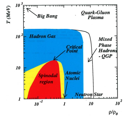
Figure 1: Phase diagram of nuclear matter: the horizontal axis shows the matter density, and the vertical axis shows the temperature. The density $\rho$ is given normalized to the saturation density $\rho_{0}$. The liquid-gas mixed phase region (yellow area) which ends up at the critical point contains the spinodal region (red area).

2.1.1 Symmetric matter

Symmetric nuclear matter is an idealized macroscopic system with an equal number of neutrons and protons. It interacts via nuclear forces, and Coulomb forces are ignored due to its size. Its density $\rho$ is spatially uniform. The nucleon-nucleon interaction is comprised of two components according to their radial interdistance : a very short-range repulsive part which takes into account the incompressibility of the medium and a long-range attractive part. Changed by five orders of magnitude the nuclear interaction is very similar to van der Waals forces acting in molecular media and consequently the phase transition in nuclear matter resembles the LG phase transition in classical fluids. However, as compared to classical fluids the main difference comes from the gas composition. For nuclear matter the gas phase is predicted to be composed not only of single nucleons, neutrons and protons, but also of complex particles like alpha-particles and light fragments depending on temperature conditions [22, 23]. In some sense, strictly speaking, one should speak of a liquid-vapour phase transition.

A set of isotherms for an equation of state (pressure versus density) corresponding to nuclear forces (Skyrme effective interaction and finite temperature Hartree-Fock theory [24]) is shown in Fig. 2. It exhibits the maximum-minimum structure typical of van der Waals equation of state. Depending on the effective interaction chosen and on the model [24, 25, 26, 27], the nuclear equation of state (EOS) exhibits a critical point at $\rho_{c}\approx$ 0.3-0.4$\rho_{0}$ and $T_{c}\approx$ 16-18 MeV. The region below the dotted line in Fig. 2 corresponds to a domain of negative compressibility: at constant temperature an increase of density is associated to a decrease of pressure. Therefore in this region density fluctuations will be catastrophically amplified until matter becomes inhomogeneous, separated into domains of high (normal) liquid density and low density gas, which finally form two coexisting phases in equilibrium. It is the so-called spinodal region and spinodal fragmentation (decomposition) is the dynamics of the phase transition. Instability growth times are equal to around 30-50 fm/c (30 fm/c = 10${}^{-22}s$) depending on density ($\rho_{0}$/2 - $\rho_{0}$/8) and temperature (0 - 9MeV) [28]. Spinodal instabilities have long been proposed as the mechanism responsible for multifragmentation [1, 29, 30].

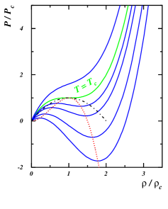
Figure 2: Equation of state relating the pressure (left) or the temperature (right) and the density (normalised to critical values) in nuclear matter. The curves represent isotherms (left) and isobars (right). The dashed-dotted lines are the boundaries of the coexistence region and the red dotted lines the boundaries of the spinodal region. From [31].

The spinodal region constitutes the major part of the coexistence region (dashed-dotted line in Fig. 2) which also contains two metastable regions: one at density below $\rho_{c}$ for the nucleation of drops and one above $\rho_{c}$ for the nucleation of bubbles (cavitation).

2.1.2 Asymmetric matter

Asymmetric nuclear matter, i.e. when the ratio of neutrons to protons is no more equal to one, is evidently a richer subject of research because its equation of state is relevant for both nuclear physics and astrophysics. In recent years, given the stimulating perspectives offered by new radioactive ion beam facilities and nuclear astrophysics, an important theoretical activity has been developed and reviews are available [32, 33, 34, 35]. Thermodynamic properties have been studied starting from non-relativistic and relativistic effective interactions and, in general, the physics is not dependent on the theoretical framework. In asymmetric matter, the energy per nucleon, i.e. the EOS, is a functional of the total ($\rho=\rho_{n}+\rho_{p}$) and isospin ($\rho_{3}=\rho_{n}-\rho_{p}$) densities. In the usual parabolic form in terms of the asymmetry parameter $I\equiv\rho_{3}/\rho=(N-Z)/A$ we can define a symmetry energy $\frac{E_{sym}}{A}(\rho)$:

$\frac{E}{A}(\rho,I)=\frac{E}{A}(\rho,I=0)+\frac{E_{sym}}{A}(\rho)I^{2}$

The first term is the isoscalar term, invariant under proton and neutron exchange, while the second (isovector) one gives the correction brought by neutron/proton asymmetry. For $I$=1 this term gives the equation of state of neutron matter. Note that because $I$ is, for most nuclei, smaller than 0.3, the isovector term is much smaller than the symmetric part, which implies that isospin effects should be rather small and all the more difficult to evidence. The symmetry term (Eq. (1)) gets a kinetic contribution directly from Pauli correlations and a potential contribution from the properties of the isovector part of the effective in-medium nuclear interactions used in models.

$$\frac{E_{sym}}{A}(\rho)=\frac{\varepsilon_{F}(\rho)}{3}+\frac{C}{2}F(\rho/\rho_{0})$$ (1)

$\epsilon_{F}$ is the Fermi energy, $F(1)$=1 and $C\approx$32 MeV. For convenience in comparing different implementations, symmetry energy is commonly approximated as :

$$\frac{E_{sym}}{A}(\rho)=\frac{C_{s,k}}{2}(\frac{\rho}{\rho_{0}})^{2/3}+\frac{C_{s,p}}{2}(\frac{\rho}{\rho_{0}})^{\gamma}$$ (2)

$\gamma$ defines the “asy-stiffness” of the EOS around normal density. The symmetry energy is said to be “asy-soft” if $E_{sym}^{pot}$ presents a maximum (between $\rho_{0}$ and $2\rho_{0}$), followed by a decrease and vanishing ($\gamma<$1) and “asy-stiff” if it monotonically increases with $\rho$ ($\gamma\geq$1). Constraining the density dependence of the symmetry energy from nuclear structure measurements, heavy ion collisions and astronomical observations is in progress [34, 35].

There are two qualitative new features of the LG phase transition in asymmetric matter. Firstly the asymmetry leads to shrinking of the region of instabilities, the spinodal region, with a reduction of critical temperature and density [27, 36] (see Fig. 4). Note a peculiarity of asymmetric nuclear matter, the direct correspondence between the nature of fluctuations and the occurrence of mechanical or chemical instabilities is lost and we face a more complicated scenario with the uniqueness of the unstable modes in the spinodal region; the instability is always dominated by total density fluctuations even for large asymmetries. This has been clearly shown in the framework of linear response theory and in full transport simulations [37, 38]. Such a result is due to gross properties of the $n/p$ interaction.

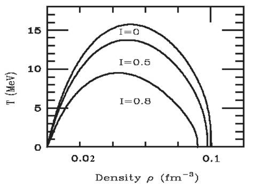
Figure 3: Spinodal boundaries in the density-temperature plane for different asymmetries $I$. Instability regions are under the curves. From [36].

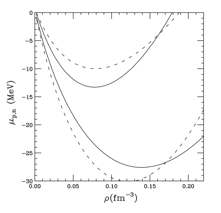
Figure 4: Density dependence, for $I$=0.2, of neutron (upper curves) and proton (lower curves) chemical potentials for asy-superstiff ($\gamma\sim$1.6 - solid lines) and asy-soft ($\gamma$=0.5 - dashed lines) EOS. From [32].

The second new feature is what is called an isospin distillation, strictly speaking neutron distillation, which produces a liquid phase composed of more symmetric matter (minimization of symmetry energy in the dense phase) and a neutron rich gas. The origin of this phenomenon is easily understood when looking at the evolution of the neutron and proton chemical potentials with density, as displayed in Fig. 4. We recall that the chemical potential is the derivative of the energy with respect to the number of particles of the system. The differences of the local chemical potentials, for neutrons and protons, which can be expressed as $\mu_{n}-\mu_{p}=4E_{sym}(\rho)I/A$, governs the mass flow in non equilibrium systems. In the density region corresponding to the LG coexistence ($\rho\lesssim 0.6\rho_{0}$, i.e. $\rho\lesssim$ 0.10 in the figure ) one can observe that neutrons and protons move in phase, both towards higher $\rho$. The slope of $\mu_{p}$ is however steeper than that of $\mu_{n}$. This means that the liquid clusters (high density) produced by bulk instability will be more symmetric while the gas phase (low density) will get enriched in neutrons. As the difference between the chemical potential slopes is more marked for an asy-soft EOS (dashed lines), the distillation effect will be stronger in that case.

2.2 From nuclear matter to hot nuclei

Evidently the hot piece of nuclear matter produced in any nuclear collision has at most a few hundred nucleons and so is not adequately described by the properties of infinite nuclear matter; surface and Coulomb effects cannot be ignored. These effects have been evaluated and lead to a sizeable reduction of the critical temperature [24, 25, 39]. Finite size effects have been found to reduce the critical temperature by 2-6 MeV depending on the size of nuclei while the Coulomb force is responsible for a further reduction of 1-3 MeV. However large reductions due to small sizes are associated with small reductions from Coulomb. Consequently, in the range $A$ = 50-400 a total reduction of about 7 MeV is calculated leading to a “critical” temperature of about 10 MeV for nuclei or nuclear systems produced in collisions between very heavy nuclei. The authors of reference [25] indicate that, due to some approximations, the derived values can be regarded as upper limits. Finally we can recall that, in infinite nuclear matter, the binding energy per particle is 16 MeV whereas it is about 8 MeV in a finite nucleus. Clearly these values well compare with the $T_{c}$ values for infinite nuclear matter and finite systems just discussed.

For finite systems composed of asymmetric matter a quantal approach has been used to determine the spinodal region [40]. A quite complex structure of the unstable modes is observed in which volume and surface instabilities are generally coupled and cannot be easily disentangled. For each multipolarity, $L$, several unstable modes appear. Fig. 6 shows, for octupole instabilities, spinodal regions in the density-temperature plane for Ca and Sn isotopes. Heavier systems have a larger instability region than the lighter ones. Moreover, more asymmetric systems are less unstable.

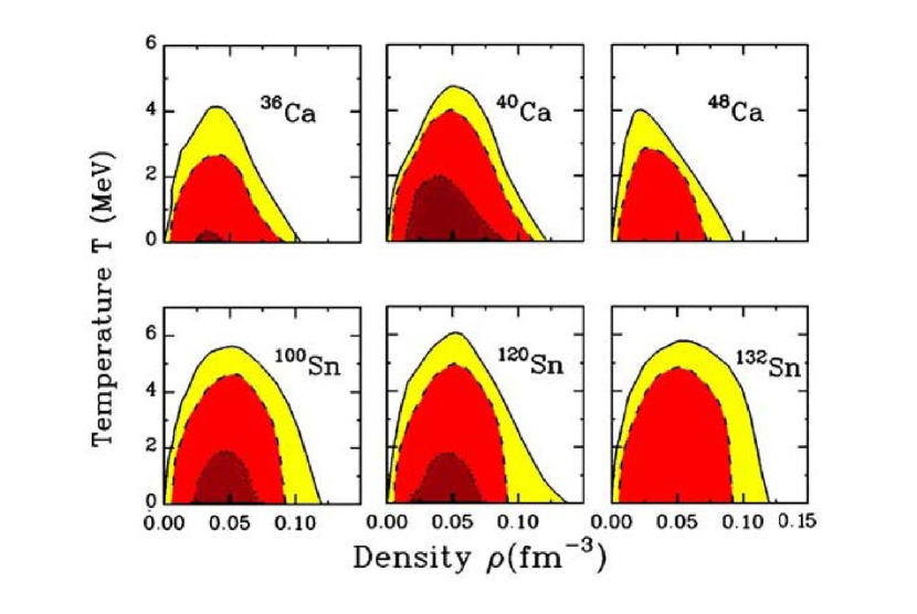
Figure 5: Spinodal border (full line) in the density-temperature plane associated to $L$ = 3, for Ca and Sn isotopes. Points having the same growth time equal to either 100fm/c (dashed) or 50fm/c (dots) are also delineated. From [40].

Figure 6: The asymmetry N/Z of the gas (circles) and of the liquid (squares) phase for central Sn+Sn collisions with different initial N/Z. Solid lines and solid symbols refer to the asystiff parametrization, and dashed lines and open symbols refer to the asy-soft parametrization. From [41].

For isospin distillation, dynamical simulations were performed for central ($b=$2 fm) symmetric Sn+Sn collisions, with masses 112, 124 and 132, at 50 MeV per nucleon incident energy [41] by using two forms of the symmetry energy in the interaction, a stiff one corresponding to $\gamma\sim$ 1.6 and a very soft one ($\gamma\sim$ 0.2-0.3). The isospin content of the liquid and gas phases (here assimilated to fragments with 3 $\leq Z\leq$ 10 and light particles, respectively) is depicted as a function of the initial $N/Z$ in Fig. 6. The fragments here are the primary hot ones. It appears that the $N/Z$ of the gas phase is larger than that of the liquid; the difference increases with the initial $N/Z$, and is larger in the asy-soft case because the symmetry energy at low density is larger. For the less neutron-rich system, the liquid phase is more neutron-rich than the gas in the asy-stiff case; this inversion is caused by Coulomb effects which become dominant over symmetry effects, leading to a strong proton emission. Finally one can notice that $I_{frag}<I_{syst}$ for n-rich systems and conversely $I_{frag}>I_{syst}$ for “n-poor” systems.

3 Applications of thermodynamic concepts to heavy-ion collisions and hot nuclei

In this section we will attempt to provide the reader with the necessary theoretical background to understand, as will be presented in the following sections, how it is possible to study a phase transition in atomic nuclei. The two major obstacles to this endeavour concern the problem of phase transitions in finite systems, and the application of statistical mechanics to processes occurring in the dynamics of finite, open systems.

Any experiment we can perform is obviously far from the thermodynamic limit: the largest possible hot nucleus/nuclear system that could conceivably be produced experimentally would have less than five hundred nucleons (²³⁸U + ²³⁸U collisions); and in actual fact is more realistically limited to $\sim$ 200 - 300 nucleons due to reaction dynamics and the Coulomb repulsion between protons. Finite (small) systems require a specific statistical mechanical treatment, for which there now exists a vast literature: apart from advances specifically concerning small systems, this includes also the wider field of statistical mechanics of systems with long-range interactions. Long-range systems interact with a potential which decays at large distances like $r^{-\alpha}$, where $\alpha\leq d$; $d$ is the dimension of the space where the system is embedded. For such systems the total energy per particle diverges in the thermodynamic limit. Small systems can be seen as a special case of the latter where the interaction range, although short, is of the order of the system size. We will try to present in this section a review of the essential aspects of this field, many of which may still be relatively new to non-practitioners.

The formation and decay of nuclear systems undergoing multifragmentation or vaporization occurs, according to various dynamical simulations (see for example [42, 43, 44]), on timescales of between a few tens and a few hundreds of fm/c ($10^{-22}-10^{-21}$ seconds). Although transport models predict that nucleon-nucleon collisions can rapidly thermalize nucleon momentum distributions at Fermi energies and above, the application of statistical equilibrium concepts seems counter-intuitive when dealing with highly-excited systems which disintegrate almost as soon as they are formed. Given that reaction products are produced on a timescale which is comparable with the time for the projectile to ‘cross’ the target, the success of equilibrium models could imply that the dynamical evolution of the system prior to multifragmentation is important only insofar as it determines the constraints which are required to characterize effective statistical ensembles in order to understand the data [45, 46]. To end this section, we will further develop these points and explain the paradigm shift required in order to progress with the identification of a phase transition in hot nuclei.

3.1 Statistical mechanics for finite systems

In the beginning was thermodynamics. Thermodynamics is an empirical science created to understand the functioning of steam engines (Carnot cycles, thermal equilibrium, entropy, etc.) - macroscopic systems with short-range interactions. Then came statistical mechanics, whose fathers (Boltzmann and Gibbs) sought to give a microscopic grounding for thermodynamics by relating the microscopic properties of $N$-body interacting systems to their macroscopic behaviour, thus introducing the concept of statistical ensembles. Most of the applications of statistical mechanics during the first century of its existence were used to explain or predict the macroscopic behaviour of matter starting from well-established microscopic interactions. These were invariably short-ranged interactions, and always in the thermodynamic limit. In this case the time-averaged properties of a single system can be calculated using a statistical ensemble of equivalent fictitious systems (the property known as ergodicity), and the physicist is free to choose whichever statistical ensemble is the easiest to work with in order to find the result (this is called ensemble equivalence).

As this situation lasted for nearly a century, it is quite natural that the assumptions that always worked in these cases lost their original significance and became seen as prerequisites for statistical mechanics to be valid. In terms of education, as these were the only cases which were widely known, they were also the only ones to be widely taught, thus perpetuating the deeply-held conviction that they were sine qua non conditions for the validity of statistical mechanics. It was mostly forgotten that statistical mechanics, as it was used and taught, was nothing but an approximation, whose validity depended on certain assumptions, such as additivity and the existence of the thermodynamic limit, which is an application of the law of large numbers.

Obviously, for macroscopic systems of particles interacting with short-range interactions, statistical mechanics (and thermodynamics) is a very good approximation; indeed the approximation is so good that it is to all intents and purposes an exact description of the macroscopic properties of such systems. In this case, using the true exact method to calculate the properties of such systems, i.e. $N$-body molecular dynamics where $N$ is of the order of the Avogadro number, would both be intractable and, frankly, overkill: there is no need to calculate the exact dynamics of such systems when 3 thermodynamic variables are sufficient to describe their behaviour with a level of precision which is far superior to the resolution of any experimental measurement.

Cracks appeared in the foundations of thermodynamics when people tried to apply it to something that was not a steam engine: for example self-gravitating systems i.e. stars [47, 48], or phase transitions in small systems such as atomic clusters [49, 50, 51, 52], and, of course, hot nuclei [9, 53]. The suggestion that such systems could exhibit a negative heat capacity when described microcanonically, whereas the canonical heat capacity is always positive by construction, thus violating ensemble equivalence, provoked a crisis of statistical mechanics which was almost of the same order as the crisis of physics itself at the turn of the twentieth century. Reactions varied from violent rejection to the conviction that the theory must quite simply be wrong, or that the apparent ensemble inequivalence must be a simple artefact due to some inappropriate approximation or hypothesis.

Nowadays, when such phenomena have been explored using many different approaches (and, in some cases, even measured) for many different systems of different types, both with long-range interactions, or, as in the case which particularly interests us in this review article, finite systems, and with a solid general theoretical grounding to explain their existence [54, 55] (even though this has only reached fruition over the last ten years), the particular properties of their statistical mechanics should no longer be an affront to the sensibilities of even the most hardened thermodynamicist.

3.1.1 Non-additivity, ensemble inequivalence and non-concave entropies

One of the most important differences between short-range and/or macroscopic systems and long-range or finite systems is non-additivity. In a macroscopic system with short-range interactions, if $X$ is some extensive variable characterizing the system (extensive quantities are proportional to the system size), then splitting the system into two (macroscopic) subsystems, $A$ and $B$, they will be characterized by the quantities $X_{A}$ and $X_{B}$, with $X_{A\cup B}=X_{A}+X_{B}$. To be more rigorous, we can write

$$\lim_{N\rightarrow\infty}X_{A}+X_{B}+X_{AB}\rightarrow X_{A\cup B}\;\mathrm{(additive)}$$

where $X_{AB}$ is the contribution from the interaction or surface between the two subsystems. In the thermodynamic limit, for short-range systems,

$$\lim_{N\rightarrow\infty}X_{AB}\rightarrow 0$$

because in this case the interaction only occurs at the surface between the two subsystems, which becomes negligible compared to the bulk for a macroscopic system.

On the other hand, for systems with long-range interactions, the interaction contribution $X_{AB}$ concerns the whole system and never disappears, even in the thermodynamic limit. For small systems, on the other hand, even if interactions are short-range, the contribution from the surface between the two subsystems can be of the same order as that of the “bulk”, and so cannot be neglected. In this case,

$$X_{A\cup B}\neq X_{A}+X_{B}\;\mathrm{(non-additive)}$$

It is important to understand the subtle difference between additivity and extensivity. Some early works on the statistical mechanics of small systems [3, 56] mistakenly identified non-extensivity as the key to understanding their behaviour, but it is in fact non-additivity which is responsible for the unusual properties of both long-range and finite systems [57]. A system may well be extensive (for example, with a total energy proportional to the number of particles in the system) and yet be non-additive (total energy of system not equal to the sum of energies of its subsystems): for example, the Curie-Weiss model of interacting spins on a lattice (see [55]). On the other hand, non-extensive systems can never be additive.

Non-additivity has profound consequences for statistical mechanics. The most important and far-reaching is the possibility for different thermodynamic ensembles to give different predictions of the system’s behaviour: this is called ensemble inequivalence [58, 59, 60]. This is at variance with the still widely-held - and widely taught - belief that the microcanonical and the canonical ensembles should always predict the same equilibrium properties of many-body systems in the thermodynamic limit. This is in fact a special case, albeit one which holds for most macroscopic systems: those with short-range interactions.

Most striking are the differences observed between microcanonical and canonical ensembles. To see how this comes about, let us first consider the textbook method to derive the canonical probability distribution by imagining a system divided into a subsystem $A$ of interest and a (much larger) subsystem $B$ which plays the role of a heat reservoir. Central to the derivation is the assumption that the energy is additive, which allows to write $E_{B}=E-E_{A}$. Obviously, when the interaction energy between subsystems $E_{AB}$ is not negligible because of non-additivity, this assumption breaks down; this does not mean that the canonical ensemble cannot be defined, however, as we will see below.

The van Hove theorem [61] states that for thermodynamic stability, thermodynamic potentials such as the entropy must be everywhere concave. If a system’s microcanonical entropy were locally non-concave in some energy interval $[E_{1},E_{2}]$, the argument goes, it would maximize its entropy (and thus recover concavity) at any intermediate energy $E=\lambda E_{1}+(1-\lambda)E_{2}$ (with $0\leq\lambda\leq 1$) by dividing into subsystems with energies $E_{1}$ and $E_{2}$ and a combined entropy $S_{12}=\lambda S(E_{1})+(1-\lambda)S(E_{2})\geq S(E)$ (in other words it would undergo phase separation). As discussed in [62, 46], van Hove’s theorem does not apply to non-additive (finite) systems. For non-additive systems phase separation at fixed energy is not possible because of the non-negligible interaction energy $E_{12}$, and therefore in the microcanonical ensemble the convex region of the entropy corresponds to equilibrium states; on the other hand, in the canonical ensemble where the energy is free to fluctuate, such states are highly improbable and practically unobservable: ensemble equivalence is violated.

3.1.2 The large deviation theoretical picture of statistical mechanics

In recent years Ellis, Touchette et al [58, 63] have provided the most comprehensive and sound basis for the understanding of the relation between ensemble inequivalence, non-concave entropies and phase transitions. Indeed, they have provided almost a re-foundation of statistical mechanics which ensures, among other things, the correct description of systems with long-range interactions, or, equivalently, finite systems, both in and out of equilibrium.

Defining statistical mechanics as a tool to find the most probable (macro)states of a random system of particles in interaction, i.e. equilibrium states, they turn to the mathematical theory of large deviations which is concerned with limiting forms of the probability distributions of fluctuations. If the probability that some random variable $A_{n}$ takes a value in the set $A$ can be expressed as

$$P_{n}(A_{n}\in A)\approx\exp-nI_{A}$$ (3)

where $I_{A}$ is a positive constant, then it is said to satisfy a large deviation principle [54]. $n$ is a parameter which is assumed to be large; it could, for example, be the number of particles or some other measure of the system size. In this case, the most probable value(s) of $A_{n}$ will be determined by the minimum(a) of the rate function, $I_{A}$, defined by the limit

$$\lim_{n\rightarrow\infty}-\frac{1}{n}\ln P(A_{n}\in B)=I_{A}$$

which must exist if Eq. (3) holds.

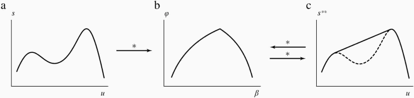
Figure 7: Ensemble inequivalence due to non-concavity of the entropy. (a) An entropy which is not concave everywhere, i.e. with a convex intruder (note that here it is the entropy per particle $s=S/N$ which is presented as a function of energy per particle $u=E/N$); (b) The LFT of $s(u)$ (represented by the arrow with an asterisk) is the (Massieu) free energy per particle $\phi(\beta)$: the non-concave part of $s(u)$ results in a non-differentiable point in $\phi(\beta)$; (c) a further LFT of $\phi(\beta)$ produces the concave hull of $s$, $s^{**}(u)$ (solid line). From [54].

Applying this theory to determine the probability of measuring the mean energy of a thermodynamic system at a given fixed value, it turns out that the rate function in this case is the (negative) microcanonical entropy, as defined by Boltzmann: in other words, the fact that the most probable (equilibrium) state of a system at fixed energy maximizes the entropy is a natural consequence of the large deviation principle, Eq. (3). Similarly, the most probable state of a system whose energy can fluctuate is determined by the minima of a rate function which is closely related to the canonical free energy.

Furthermore in this framework the canonical free energy (or, more precisely, the Massieu potential $\Phi(\beta)=\beta F(\beta)$) is obtained quite naturally from the microcanonical entropy by a Legendre-Fenchel transform (LFT)

$$\Phi(\beta)=\inf_{E}\left[\beta E-S(E)\right]$$ (4)

which is valid even if the entropy $S(E)$ is non-differentiable, and whether or not it is everywhere concave. If $S(E)$ is everywhere concave, it can be obtained by LFT from the canonical free energy:

$$S^{**}(E)=\inf_{\beta}\left[\beta E-\Phi(\beta)\right]$$ (5)

i.e. if $S(E)$ is everywhere concave, $S^{**}(E)=S(E)$. In this case, the canonical and microcanonical ensembles are equivalent at the thermodynamic level.

For entropies which are not everywhere strictly concave, $S^{**}(E)$ is the concave hull of $S(E)$, i.e. in this case the full physics of the microcanonical ensemble cannot be deduced from the canonical ensemble. This is illustrated in Fig. 7, taken from [54]. Ensemble non-equivalence therefore arises from the mathematical properties of the Legendre-Fenchel transform, and the occurrence of non-concave entropies. As a general consequence, when entropies are everywhere concave, the ensembles are always equivalent and one ensemble is as good as another when calculating thermodynamics of a system. On the other hand, ensemble inequivalence arises every time that entropy is not strictly globally concave.

3.1.3 First order phase transitions in finite systems

According to the Ehrenfest definition, the canonical free energy function $\phi(\beta)$ of Fig. 7(b) is that of a first-order phase transition, as it presents a discontinuity in its first-order derivative. The microcanonical entropy obtained by LFT from this free energy (full line in Fig. 7(c)) is that of a first-order phase transition for an additive system, which in the presence of short range interactions means in the thermodynamic limit. For these systems, in a certain range of energies, the entropy of the system is greater when it is divided into two different homogeneous phases than if it contains a single homogeneous phase: a section of constant slope in the entropy appears in this energy range because the total entropy is obtained by a linear combination of the entropies of the two phases. This linear segment corresponds to a constant temperature as the system is transformed from one phase into the other, For these systems ensemble equivalence is not violated (strictly speaking, the ensembles are said to be partially equivalent, as, while never convex, the entropy is not everywhere strictly concave).

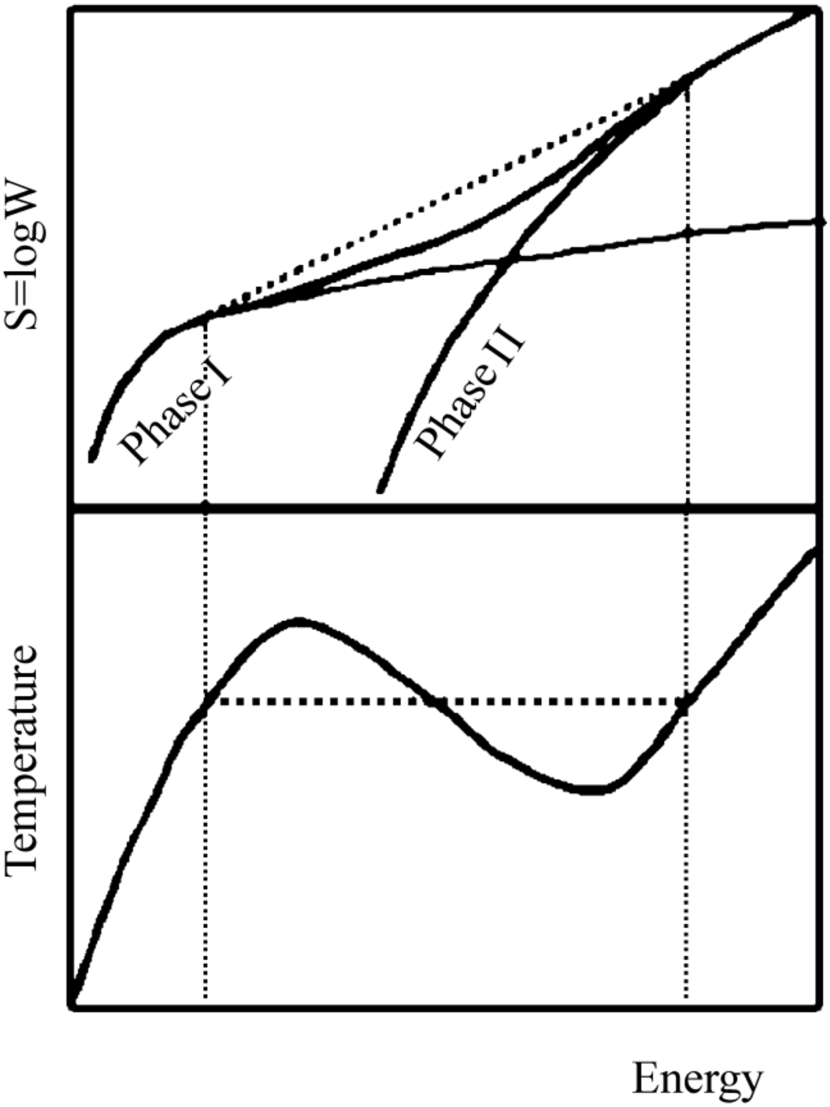
Figure 8: Schematic description of a first-order phase transition in a finite system as the sudden opening of a new disordered phase at a certain threshold energy. From [64].

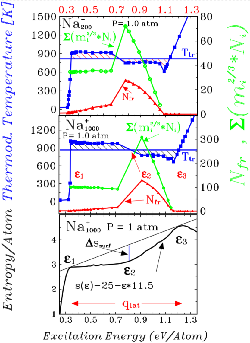
Figure 9: Top two panels: (blue squares) constant pressure microcanonical caloric curves for atomic clusters of 200 or 1000 atoms; (red triangles) number of fragments $N_{fr}$ with $m_{i}\geq 2$ atoms; (green triangles) effective number of surface atoms $\sum_{m_{i}\geq 2}(N_{i}m_{i}^{2/3})$. Bottom panel: the microcanonical entropy for $Na_{1000}^{+}$ clusters showing the entropy deficit $\Delta s_{surf}$ due to the increase in effective surface area of the inhomogeneous fragmented system. From [65].

The microcanonical entropy with a convex intruder shown in Figure 7(a) is typical of a first-order phase transition in non-additive systems, as was first realized in the specific case of the melting of finite atomic clusters [62, 49, 66, 50] and later developed in the field of phase transitions for hot nuclei [9, 67]. These studies are of particular interest because in the case of rare gas atoms interacting through a Lennard-Jones potential the thermodynamic phase transition is the well-known first order solid-liquid transition. It can be rigorously shown that the behaviour associated with the convex entropy function of the finite systems is the embryonic precursor of the infinite system phase transition [52].

For finite clusters of between 13 and 147 argon atoms, the solid-liquid transition occurs without phase separation: in the “coexistence” region corresponding to energies where the entropy is convex, the clusters are either all “solid” or all “liquid” [49], where the two phaselike forms can be distinguished energetically (either at different times when considering the dynamical evolution of a single cluster, or in different clusters when considering a statistical ensemble). As mentioned above, these clusters are too small to support coexistence of multiple phases inside the same system, and therefore cannot “heal” their convex entropy by mixing the two together. Rather, the different thermodynamic phases of matter first manifest themselves microscopically as distinct regions of phase space with their own characteristic temperatures, separated by an energy barrier [50]. Indeed, the first premises of a first-order phase transition at a microscopic level can be seen as the sudden opening of a new disordered phase at a certain threshold energy (see Fig. 9), with an entropy which increases much faster than that of the ordered phase [68, 64],

$$\left(\frac{\partial S}{\partial E}\right)_{\mathrm{disordered}}>\left(\frac{\partial S}{\partial E}\right)_{\mathrm{ordered}},$$

creating a convex intruder in the total entropy of the system. As $\partial S/\partial E$ is of course nothing but the inverse temperature, this implies a lower temperature for the higher energy disordered phase at the onset, and indeed such transitions are always accompanied by back-bending caloric curves where the temperature first decreases before resuming a monotonic increase in the disordered phase [49, 50].

Gross studied the embryonic liquid-gas transition for metallic clusters of 200 to 3000 atoms [65]. They manifest another way in which a finite system can undergo a phase transition of this type without bulk phase coexistence: the clusters undergo fragmentation into a mixture of smaller clusters (fragments) and monomers. Fig. 9 shows two examples of the evolution of the number of fragments $N_{fr}=\sum_{m_{i}\geq 2}N_{i}$ with energy for the clusters $Na_{200}^{+}$ and $Na_{1000}^{+}$. Within the transition region (i.e. between the energies $\epsilon_{1}$ and $\epsilon_{3}$) $N_{fr}$ steadily increases, reaches a maximum and then decreases as all fragments are transformed into monomers. The effective increase in the amount of surface in this inhomogeneous system due to the presence of the fragments is represented by the total number of surface atoms in the fragments, $\sum_{m_{i}\geq 2}(N_{i}m_{i}^{2/3})$ (green curve in Fig. 9). Like $N_{fr}$, it too reaches a maximum inside the transition region, and leads to an entropy decrease $\Delta s$ with respect to the concave hull which would be achieved for bulk phase coexistence (bottom panel in Fig. 9). The microcanonical entropy therefore presents a convex intruder which signals the presence of a first-order phase transition.

As system size increases, but still far from the thermodynamic limit, it will be constituted of sufficient bulk material so that different phase regions can coexist within it. However some non-additivity still remains as long as $N<\infty$: in this case although the part of the entropy corresponding to the bulk (which increases like $N$) is maximized by the phase coexistence, there are other terms which increase with the size of the interphase surface (which increases like $N^{(d-1)/d}$, i.e. $N^{2/3}$ in 3 dimensions). The surface contribution must be negative: if not, the surface area would maximize and the two phases would become one fog-like phase [62]. The size of the surface depending on the proportions of the two phases, it will first increase with energy, reach a maximum when each phase occupies 50% of the bulk, and then decrease as the energy increases further. The entropy of a finite two-phase system will therefore fall below the concave hull shown by the full line in Figure 7(c), and present a convex intruder rather like the dashed line in the same figure; the convexity disappears (for systems with short-range interactions) as the thermodynamic limit is approached, like $N^{2/3}/N\sim N^{-1/3}$. It is interesting to note here a subtle point made by Gross [69]. Although the entropy per particle regains its concavity in the thermodynamic limit, the curvature of the total entropy $S$ = $S_{vol}-\Delta S_{surf}$ will remain positive in the transition region as the bulk entropy $S_{vol}$ is the concave hull with zero curvature. Therefore the overall curvature is given by $-\partial^{2}\Delta S_{surf}/\partial E^{2}$. To quote Gross, “the ubiquitous phenomena of phase separation exist only by this reason” [69]. However it should be remembered that in the strict thermodynamic limit the total entropy is diverging and only the entropy per particle makes sense. In any case, for finite systems, however large, the convex region is always present.

3.2 Pseudo-equilibrium

It was Bohr who introduced statistical mechanics to nuclear physics [70] and Weisskopf who introduced concepts of nuclear temperature and entropy with the theory of neutron evaporation from “excited” nuclei [71]. In the framework of the compound nucleus picture they developed, statistical equilibrium is justified by the clear separation of timescales between the formation of a compound nucleus, its equilibration, and subsequent decay. As pointed out in the introduction to this section, in collisions at the energies required for multifragmentation or even vaporization, the separation of timescales for formation and decay of hot nuclei is not always so clear, and yet models based on classical equilibrium statistical mechanics are extremely successful in reproducing or even predicting many observables for these reactions.

A statistical treatment is justified whenever a very large number of microstates exists for a given set of observables. This is always the case for the output of a collision, meaning that at least in principle a statistical approach should always be successful. An ensemble of events coming from similarly prepared initial systems and/or selected by sorting always constitutes a statistical ensemble [46]. To use classical equilibrium statistical mechanics requires an adequate definition of the relevant microstates i.e. just that information which ineluctably entails the production of a given macroscopic event [45]. For the multibody decay of hot nuclei, the microstates relevant to a statistical description correspond to the microscopic configuration of each reaction at the freeze-out instant: this is defined as the time after which the characteristics of the fragments and particles produced in the reaction will no longer significantly change, apart from the effects of secondary decay (evaporation of light particles due to residual excitation energy) and Coulombian acceleration due to mutual repulsion between charged fragments.

Statistical equilibrium means that the probabilities, $\{p_{i}\}$, of each microstate compatible with the constraints placed upon the system (conservation laws, etc.) maximize the associated statistical entropy,

$$S=-\sum_{i}p_{i}\log p_{i}+\sum_{X}\lambda_{X}<X>$$ (6)

where the set of $<X>$ are the constraints and $\lambda_{X}$ are the associated Lagrange multipliers [64, 72]. In this case we say that the available phase space is uniformly populated. Any set of microstates for which this population is achieved given a certain set of constraints corresponds to statistical equilibrium at the level of the corresponding statistical ensemble. In the case of hot nuclei, we are dealing with an ensemble of freeze-out configurations produced by many different collisions. For the application of statistical equilibrium approaches it is unimportant whether each individual collision had achieved equilibrium at the freeze-out instant, it is only required that the ensemble of realized configurations be equivalent to a random sample taken from the available phase space. This can be achieved by the chaotic nature of the dynamics of the reactions which in addition are averaged over many different initial conditions in order to constitute an ensemble of events that covers the phase space uniformly [46], all the more so if the portion of phase space in question is well-defined, i.e. when ensembles are built from homogeneous event selections. To quote the fathers of the first statistical model of composite fragment production in the 20-200 MeV per nucleon bombarding energy range, Randrup and Koonin, “it is not necessary to argue that equilibrium be reached in any given collision, since a statistical occupation of the phase space at the one-fragment inclusive level can occur as a result of averaging over many separate collision events, each of which can be far from equilibrium throughout” [73]. This approach has been called pseudo-equilibrium [45].

It is important to underline the change of paradigm associated with this approach. Early on in the development of statistical models for multifragmentation, Gross suggested that equilibrium might be achieved at the level of each reaction by “chaotic mixing” [74], a sufficiently intense period of nucleon and energy exchange between the strongly-interacting nascent fragments as the system expands towards freeze-out. However, as Cole has pointed out [45], this is a strong hypothesis which can in addition unnecessarily complicate the interpretation of results. Instead we concern ourselves only with the equilibrium of statistical ensembles composed of the systems at freeze-out; more precisely, as exact equilibrium is a theoretical abstraction which cannot be achieved in the real world, our statistical ensemble need only be sufficiently close to equilibrium for most observable properties to be consistent with a uniform population of the phase space. Residual effects which are directly linked to the collision dynamics may then reveal themselves in the fine details of the comparison between model and data.

Before leaving this topic, let us point out an important aspect which should not be forgotten: the statistical ensembles built from systems at freeze-out are not ergodic. There is no equivalent single system which would evolve over time through the ensemble of microstates of the ensemble. If we were to “unfreeze” any of the systems in our ensemble and let time run on, obviously the particles and fragments would immediately continue their flight toward the detectors; even if we were to take one and put it in a (very small) box to try to keep it in the freeze-out configuration, it would soon cease to resemble any of the other systems of the statistical ensemble, the Coulomb repulsion forcing the charged fragments against the walls of the box. And yet, at the level of the statistical ensemble, it is perfectly possible to speak of a well-defined characteristic volume, $<V>$, or mean square radius $<R^{2}>$. The associated Lagrange multiplier (see Eq. 6) $\lambda_{V}=\beta p$, thereby defining the pressure at the level of the ensemble. Therefore defining thermodynamic properties for dynamically evolving open systems is not a problem with this approach. The non-ergodicity is not a problem per se for the validity of the approach, but tends to disturb the unwary as it is at odds with the usual approach where a thermodynamic system is represented by a fictitious statistical ensemble. When studying a phase transition in hot nuclei, the statistical ensemble is real and phase transition is evidenced from the thermodynamics of the ensemble.

3.2.1 Effective statistical ensembles

The starting point for our studies of nuclear thermodynamics is therefore a statistical ensemble prepared by the dynamics of collisions. The question is then: which ensemble is best suited to a study of the thermodynamics of hot nuclei?

One might be tempted to reply that the microcanonical ensemble is most apt, as it describes isolated systems of fixed energy and particle number. However this is not necessarily adapted to the data we have to analyse. The closest we could come to such a situation would be in the case of hadron-induced reactions such as $\pi^{+/-}+X\rightarrow Y*$. Even so, it could be pointed out that the thermodynamic microcanonical ensemble is defined not only for fixed $E$, $N$ but also $V$. For systems undergoing a LG phase transition the volume $V$ is an essential degree of freedom. At best, an average size of the fragmented systems at freeze-out can be inferred from experimental observables. Indeed the volume is not fixed but multiplicity and partition-dependent. From the theoretical point of view one is therefore forced to consider a statistical ensemble for which the volume can fluctuate from event to event around an average value [8]. One comes to a microcanonical isobar ensemble in which the average freeze-out volume is used as a constraint [75, 72], defined through the partition function

$$Z_{\lambda}(E)=\sum_{V}W_{V}(E)exp(-\lambda AV),$$ (7)

with the density of states $W_{V}(E)$ having energy $E$ and volume $V$ with $A$ particles. In this ensemble the $E$ and the Lagrange conjugate of the volume observable $\lambda$ represent the two state variables of the system. This is not the microcanonical ensemble defined by the entropy $S=logW_{V}(E)$ and to avoid misunderstandings, one should note the temperature, pressure and average volume by $T_{\lambda}$, $P_{\lambda}$ and $<V>_{\lambda}$ with the associated Lagrange multiplier $\lambda$ = $P_{\lambda}$ / $T_{\lambda}$.

The choice of statistical ensemble is best determined by the data. When one is not interested in an event-by-event analysis and only wants to calculate mean values at very high excitation energies ($\geq$ 8 - 10 MeV per nucleon) where the number of particles associated to deexcitation is large [76, 77, 78, 8, 79] (see 5.2), then it is clear that a grand-canonical approach is most suited. The grandcanonical or macrocanonical ensemble corresponds to the rougher description where the number of particles as well as energy of the systems can fluctuate. In this ensemble the temperature and the chemical potential are fixed variables. Constraints are only on the average mass and charge of the systems. On the other hand to perform analyses on an event-by-event basis or to study, for example, partial energy fluctuations (see 6.1.2) the microcanonical ensemble, is the relevant one. It is used to describe a system which has fixed total energy and particle number [80, 74, 8, 81]. In this ensemble the temperature is no longer a natural concept and a microcanonical temperature can be introduced through the thermodynamic relation: $T_{micro}^{-1}=\partial S/\partial E$. Results have to be discussed as a mixing of microcanonical ensembles in order to be compared to those of canonical ensembles. Numerical realizations are possible after elaborating specific algorithms based on the Monte Carlo method. Finally one can conclude about the choice of the different ensembles by saying that the excitation energy domain, the pertinent observable to study and the event sorting chosen impose the dedicated statistical ensemble to be used. For comparison with data additional constraints (volume, pressure, average volume…) are added; they correspond with associated Lagrange multipliers to isochore and isobar ensembles [82, 75].

4 How to study a phase transition in hot nuclei

If experiments benefit from a large variety of nuclear collisions to produce and study hot nuclei, it is essential to underline the importance of the mutual support between theory and experiments to progress on the complex subject of phase transition for hot nuclei. To illustrate this, Fig. 10 shows how theory gives precious information on trajectories in the phase diagram for central collisions leading to quasifusion. One learns immediately that after a compression phase due to the initial collisional shock a subsequent expansion occurs leading to the mixed phase region. We will see all along this review how this mutual support is present for most of the aspects and especially to better specify the thermodynamic variables: excitation/thermal energy, temperature, pressure, density or average volume at freeze-out.

Among the existing models some are related to statistical descriptions based on multi-body phase space calculations whereas others describe the dynamic evolution of systems resulting from collisions between nuclei via molecular dynamics or stochastic mean field approaches The first approach uses the techniques of equilibrium statistical mechanics with the freeze-out scenario defined in section 3.2 and has to do with a thermodynamical description of the phase transition for finite nuclear systems. The second, in principle more ambitious, completely describes the time evolution of collisions and thus helps in learning about nuclear matter (stiffness of the effective interaction and in-medium nucleon-nucleon cross-sections), its phase diagram, finite size effects and the dynamics of the phase transition involved.

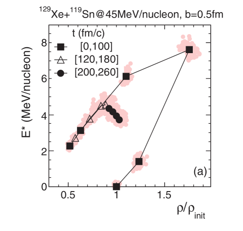
Figure 10: Mean trajectory in the phase diagram plane (density - excitation energy) for central collisions between Xe and Sn nuclei; each black marker stands for a time from $t$ = 0 to $t$ = 260 fm/c by a step of 20 fm/c (30 fm/c = 10^-22s). From [43].

4.1 A large choice of collisions to produce hot nuclei

Experimentally to study a phase transition in hot nuclei we dispose of heavy-ion collisions at intermediate and relativistic energies and hadron-nucleus collisions at relativistic energies. Investigations must apply to homogeneous samples of events, which requires an appropriate sorting mandatory for thermodynamical purposes (section 3.2). In hadron-nucleus collisions all events have similar topological properties independently of the impact parameter, as a single hot nucleus is created after a more or less abundant preequilibrium emission. Conversely, in heavy-ion collisions, the outgoing channel is different depending on the masses and asymmetry of the incident partners, the incident energy and the impact parameter. At intermediate energies residual interactions (nucleon-nucleon collisions) strongly compete with mean field effects; the number of nucleon-nucleon collisions largely fluctuates, leading to different final reaction channels for the same initial conditions. The weakening of the mean field hinders, on average, full stopping above about 30 MeV per nucleon incident energy; the large fluctuations mentioned above allow however the observation of ”quasifusion” at higher energies, although with small cross sections [83]. Most of the collisions end up in two remnants coming from the projectile and the target, what we call quasi-projectile and quasi-target - accompanied by some evaporated particles -, and some fragments and particles with velocities intermediate between those of the remnants: these are called mid-velocity products. They may have several origins, e.g. direct preequilibrium emission from the overlap region between the incident partners, or a neck of matter between them which may finally separate from quasi-projectile or quasi-target, or from both. At relativistic energies, mean field effects being negligible, a geometrical picture - the participant-spectator model - [84, 85] well describes mid-peripheral and peripheral collisions which lead to what are called projectile and target spectators instead of quasi-projectiles and quasi-targets at lower incident energies [86]. Whatever the type of reaction, a fraction of the incident translational energy is transformed into “excitation energy”, $E^{*}$, which may be shared into thermal energy (heat) and collective energies. While experimental calorimetry gives a direct access to $E^{*}$, knowing how it is shared between thermal or collective energies relies on models. The sorting of events measured with powerful multidetectors is generally done using global variables, which serve to condense the large amount of information obtained for each event. Ref. [87] well illustrates how to carefully select hot nuclei of similar sizes produced in central (quasifusion) and semi-peripheral (compact quasi-projectiles) collisions. Two philosophies guide the methods used for event sorting: the impact parameter dependence, and the event topology. Details can be found in [13].

To conclude on this part one can say that with central heavy-ion collisions at intermediate energies leading to quasifusion one can select a well defined set of events for each incident energy. For semi-peripheral and peripheral heavy-ion collisions at both intermediate and relativistic energies and hadron-nucleus collisions at relativistic energies one can follow, with a single experiment, the evolution of deexcitation properties of hot quasi-projectiles, projectile spectators and selected hot nuclei over a large excitation energy domain through specific variables like, for example, the size of the heaviest fragment (quasi-projectiles) or the charge bound in fragments (projectile spectators). On the theoretical side statistical and dynamical models are first used to qualitatively learn about collisions. Then, results of models are quantitatively compared to experimental data. Models are also used to bring complementary information when it is missing from experiments.

4.2 Statistical models

As we will see all along the following sections, a large variety of statistical models are used to predict and support experimental observations related to a phase transition in hot nuclei and to give complementary information to data when needed. The present subsection makes a brief presentation of those models and gives their spirit.

4.2.1 Fundamental statistical models and Fisher droplet model

In this class of models we group those which are not specifically nuclear in nature: (i) percolation model, (ii) Ising, lattice gas and Potts models, which are used in the study of a phase transition in hot nuclei to derive qualitative or semi-quantitative behaviours, (iii) the Fisher droplet model used in a more quantitative way to extract critical - pseudo critical information and free energy. We refer to section 6 for applications of these models.

Percolation, Ising, lattice gas and Potts models

Percolation [88] is the simplest example of a model that displays critical behaviour. It is purely geometrical and can be described as a grid of Euclidian dimension $d$ in which the nodes are randomly populated with probability $p$, which is called site percolation. If instead of the nodes we activate the intranode links with probability $p$ one speaks of bond percolation. Site-bond percolation processes are those in which $p$ is different from 1. In such a model the phase transition or the critical point is related to the appearance in the system of a percolating (single) cluster. In such a cluster a set of nearest-neighbour sites or bonds are active, that goes from - $\infty$ to + $\infty$. For a finite system with a given geometry like a box, a possible definition of percolating cluster is that there exists a set of nearest-neighbour occupied sites (activated bonds) that extends from one side of the box to the opposite one (other definitions can also be used). For infinite systems there exists a sharp critical bond activation probability $p_{c}$ such that for $p$ above $p_{c}$ the probability of finding a percolating cluster is 1, whereas below $p_{c}$ the probability of finding such a cluster is 0. For finite lattices the transition from one regime to the other is smooth. The order parameter for this model is $P_{\infty}$ which is the fraction of occupied nodes that belong to the percolating cluster and the distance from criticality $\epsilon$ is ($p$ - $p_{c}$). Since sites/bonds are empty with probability (1 - $p$), the probability of a node to belong to the infinite cluster is $p$.$P_{\infty}$ and the probability of belonging to a finite cluster is $\sum_{s}s.n_{s}$ where $n_{s}$ is the yield of the occupied boxes of size $s$. The critical properties of percolation are represented by the singular behaviour of moments of the cluster size distribution which are expressed as a function of ($p$ - $p_{c}$) (or its absolute value) with exponents that contain critical exponents $\sigma$, $\beta$, $\gamma$ and $\tau$ related among them.

A remarkably successful model of an interacting system is the Ising model. A classical spin variable $s_{k}$, which is allowed to take values $\pm$1, is placed on each site of a regular lattice, under the influence of an external magnetic field $h$ and a constant coupling $J$ between neighbouring sites according to the Hamiltonian

$$\mathcal{H}_{IS}=-h\sum_{k=1}^{N}s_{k}-\frac{J}{2}\sum_{k\not=j}^{N}s_{k}s_{j},$$

where the second sum extends to closest neighbours.

The Ising model was originally introduced to give a simple description of ferromagnetism. In reality the phenomenon of ferromagnetism is far too complicated to be treated in a satisfactory way by this oversimplified Hamiltonian. However the fact that the Ising model is exactly solvable in 1$d$ and 2$d$ and that very accurate numerical solutions exist for the three dimensional case makes this model a paradigm of first and second order phase transitions. The other appeal of the Ising model is its versatility. It is why it is also well adapted to describe fluid phase transitions. One can show that a close link exists between the Ising hamiltonian and the lattice gas Hamiltonian, which is the simplest modelization of the LG phase transition

$$\mathcal{H}_{LG}=\frac{1}{2m}\sum_{k=1}^{N}p_{k}^{2}n_{k}-\frac{\epsilon}{2}\sum_{k\not=j}^{N}n_{k}n_{j}.$$

In the lattice gas model, the same N lattice sites in $d$ dimensions are characterized by an occupation number, $n_{k}$ = 0,1, and by a $d$ component vector $\overrightarrow{p_{k}}$. Occupied sites (particles) interact with a constant closest neighbour coupling $\epsilon$. For nuclei the coupling constant $\epsilon$ = - 5.5 MeV is fixed so as to reproduce the saturation energy. The relative particle density $\rho$/$\rho_{0}$ is defined as the number of occupied sites divided by the total number of sites and is linked to the mean magnetization of the Ising model, $M$, by $\rho$/$\rho_{0}$ = 2$M$ - 1. Different choices can be made to measure the average volume of the system. The most natural measure is obtained by averaging on the set of events with, for each event $e$, the volume observable proportional to the cubic radius

$$V^{(e)}=\frac{4\pi}{3A}\sum_{i=1}^{N}r_{i}^{3}n_{i},$$

where $r_{i}$ is the distance to the centre of the lattice, $n_{i}$ is the occupation number and $A$ is the number of particles. Even for simplified models such as the Ising model no analytical solution exists for a number of dimensions larger than 2. This is the reason why mean field solutions have been developed [72]. Moreover the exact solution of three dimensional Ising-based models can only be achieved through numerical Metropolis simulations [89].

Another classical spin model is the Potts model. To define this model a $q$-state variable, $\sigma_{i}$ = 1, 2, 3… $q$, is placed on each lattice site. The interaction between the spins is described by the Hamiltonian

$$\mathcal{H}=-J\sum_{<ij>}\delta_{\sigma_{i}\sigma_{j}}.$$

$\delta$ is a Kronecker delta-function so the energy of two neighbouring spins is -$J$ if they are in the same state and zero otherwise. Thus, the Potts model has $q$ equivalent ground states where all the spins are identical but can take any one of the $q$ values. As the temperature is increased there is a transition to a paramagnetic phase which is continuous for $q\leq$ 4 but first-order for $q>$ 4 in two dimensions.

Fisher’s model

M.E. Fisher [90] proposed a droplet model to describe the power law behaviour of the cluster mass distribution around the critical point for a LG phase transition. The vapour coexisting with a liquid in the mixed phase is schematized as an ideal gas of clusters, which appears as an approximation to a non-ideal fluid. This model was applied early on to multifragmentation data [91, 92] by considering all fragments but the largest in each event as the gas phase, the largest fragment being assimilated to the liquid part. The yield of a fragment of mass A reads:

$$\mathrm{d}N/\mathrm{d}A=\eta(A)=q_{0}A^{-\tau}\exp((A\Delta\mu(T)-c_{0}(T)\varepsilon A^{\sigma})/T).$$ (8)

In this expression, $\tau$ and $\sigma$ are universal critical exponents, $\Delta\mu$ is the difference between the liquid and actual chemical potentials, $c_{0}(T)\varepsilon A^{\sigma}$ is the surface free energy of a droplet of size A, $c_{0}$ being the zero temperature surface energy coefficient; $\varepsilon=(T_{c}-T)/T_{c}$ is the control parameter and describes the distance of the actual to the critical temperature. At the critical point $\Delta\mu=0$ and surface energy vanishes: $\eta(A)$ follows a power law. Away from the critical point, but along the coexistence line $\Delta\mu=0$, the cluster distribution is given by: $\mathrm{d}N/\mathrm{d}A=\eta(A)=q_{0}A^{-\tau}\exp((-c_{0}(T)\varepsilon A^{\sigma})/T)$.
The temperature $T$ is determined by assuming a degenerate Fermi gas. The probability of finding a fragment of mass $A$ can be equivalently and directly calculated from the free energy. For constant pressure statistical ensembles, the Gibbs free energy is the suitable quantity to look at, while for a constant volume ensemble (as assumed in many models) the Helmhotz free energy is the relevant one. One or the other prescription gives some differences especially above the critical point. Assuming a free energy $F$, the mass yield near the critical point can be written $\eta(A)=y_{0}A^{-\tau}\exp(-F/T)A$. If one introduces the two constituents, neutrons and protons, a mixing entropy term appears in the mass-atomic number yield. Details can be found in [93].

4.2.2 Models of nuclear multifragmentation

In this class of models we group those which take into account specific nuclear properties such as binding energies, level densities, surface tension, etc. i.e. models whose physical picture is that of the production of multiple nuclear fragments, as opposed to generic clusters. The starting point for such models is the freeze-out instant previously described in section 3.2. A highly-excited nuclear system will arrive, at some point in its evolution, at a moment commonly known as the freeze-out after which the characteristics of the fragments produced by its decay will no longer significantly change. This is a more than reasonable assumption: in fact, if we “play the film in reverse” and imagine the final detected products flying back out of the detectors towards the target, it is clear that such an instant must exist. The freeze-out configuration is commonly assumed to correspond to a moment at which all fragments produced in the break-up have moved sufficiently far apart so that they are outside of the range of the nuclear interaction; otherwise they would experience further dissipative interactions and possibly nucleon exchange with their neighbours, as is well known from the study of dissipative nuclear reactions in the deep-inelastic regime [94, 95, 96, 97]. This, too, is a reasonable assumption.

The main hypothesis of these models is that the final products can be calculated based only on the available phase space at freeze-out, given a set of constraints such as the total numbers of neutrons and protons, total energy, angular momentum, etc. (any of which may, depending on the model, be fixed or allowed to fluctuate). Specific models differ in their description of the freeze-out configuration, the implementation of the initial conditions (constraints), and the numerical methods employed to make predictions based on the corresponding ensembles. In the following we will try to present the most important distinguishing aspects of the most successful and well-used models.

The pioneering work of Randrup and Koonin [73] is commonly recognized to be the first example of such a model, but it suffered from limitations such as only treating the production of light clusters using a grand-canonical approach, and was therefore limited to excitation energies well above the phase transition domain. Subsequent models acknowledged and built upon this work in order to treat more realistically aspects such as the role of the Coulomb repulsion and the production of heavy fragments, to be able to explore the predicted coexistence region.

The Copenhagen model (SMM)

The Statistical Multifragmentation Model (SMFM [98, 99, 8]), more commonly known as SMM, is one of the most widely used statistical models for the interpretation of nuclear multifragmentation data. It describes the break-up/multifragmentation of an ensemble of excited nuclear systems $(A_{0},Z_{0})$ into partitions $\{N_{AZ};1\leq A\leq A_{0},0\leq Z\leq Z_{0}\}$. The freeze-out stage consists of hot fragments and nucleons or light clusters ($A<4$) occupying a volume $V$ in thermal equilibrium characterized by a temperature $T$. After their formation in the freeze-out volume, the fragments propagate independently in their mutual Coulomb fields and undergo secondary decays. The deexcitation of the hot primary fragments proceeds via evaporation, fission, or via Fermi break-up for primary fragments with $A\leq 16$.

The break-up volume $V=(1+\kappa)V_{0}=(1+\kappa)A_{0}/\rho_{0}$ is taken large enough so that no fragments overlap; typical values are $\kappa\approx 2$, i.e. $V\approx 3V_{0}$. $V_{0}$ is the volume of a nucleus of mass $A_{0}$ at normal density. The hot fragments ($A\geq 4$) are spherical droplets at normal nuclear density, whose free energy is described by a charged liquid drop parametrization containing bulk, symmetry, surface and Coulomb terms. The bulk term contains a Fermi gas dependence on temperature. The surface term vanishes at the critical temperature of infinite nuclear matter, usually taken to be $T_{C}=18$ MeV. The partition temperature $T$ is determined in order to conserve energy from one partition to another. The free energy component associated with thermal motion of fragments depends on a “free” volume $V_{f}=\chi V_{0}$ in which they can move without overlapping. $\chi$ depends on the multiplicity of the partition and typically varies between 0.2 and 2. The assumption of thermal equilibrium means that a single temperature $T$ is used to characterize both the fragments’ momenta and their internal excitation energy, but the degree of equipartition can be modified by treating the inverse nuclear level density parameter $\epsilon_{0}=A/a$ which appears in the bulk component of the fragment free energy as a free parameter: setting $\epsilon_{0}=\infty$ results in a hot gas of cold fragments with zero excitation energy.

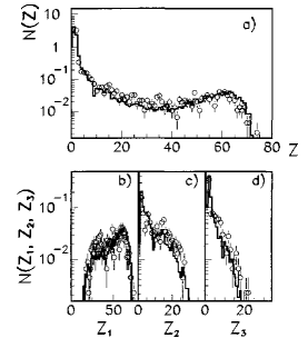
Figure 11: Comparison of experimental mean elemental fragment multiplicity, $N(Z)$ and distribution of the three heaviest fragments (Z₁, Z₂ and Z₃) in each event (quasi-projectile hot nuclei produced in peripheral - 0.8$<b/b_{max}\leq$0.9 - ¹⁹⁷Au + ¹⁹⁷Au collisions at 35 MeV per nucleon incident energy with fission events removed) with SMM simulations. The circles show experimental data and the lines the SMM predictions filtered by the experimental device. From [100].

Figure 12: Comparison of experimental data (Xe+Sn quasifusion hot nuclei produced in central collisions at 32 MeV per nucleon incident energy) with SMM simulations. The lines are for data and symbols for filtered SMM predictions (all fragments, except open circles and dashed lines which refer to the largest fragment of each partition). Z_bound represents the sum of the charges of all fragments. From [101].

In the original version of the model [8], partition generation was performed using a Monte Carlo method. All possible partitions with low ($M\leq 3,4$) multiplicity are directly generated and the associated mean multiplicity calculated using their microcanonical statistical weights. If the calculated mean multiplicity $<M>$ is small enough, one of these partitions is randomly selected to generate an event. If not, a partition with larger multiplicity is generated starting from the grand-canonical expression for $<N_{AZ}>$ calculated from the free energy of the partition. It should be noted that in this version of the model the Coulomb interaction between fragments was approximated in a Wigner-Seitz approach.

A later improvement to the model was the introduction of Metropolis sampling, using the so-called “Markov chain” approach to efficiently generate partitions representative of the whole phase space [102]. Starting from a partition of multiplicity $M$ a new distinct partition is generated by moving one nucleon of the partition: this corresponds to either emission or absorption of a free nucleon by one of the fragments, or to transfer of a nucleon from one fragment to another. This procedure was shown to significantly improve the quality of the statistical sampling compared to the previous method. Moreover, it allows to calculate directly the Coulomb contribution for each break-up channel based on actual fragment coordinates in the freeze-out volume, and to explicitly include conservation of angular momentum in the model; recently this has allowed to begin systematic theoretical investigations of the Coulomb and angular momentum effects on multifragmentation in peripheral heavy-ion collisions at Fermi energies, especially on the isotope yields, which are crucial for astrophysical applications [103].

Radial expansion velocities, fully decoupled from thermal properties, were also added for a better comparison with experiments. As for the “Big Bang” a self similar expansion (collective velocity proportional to r) is observed up to around 80 - 100 fm/c after the beginning of central collisions in all dynamical models and this is why this prescription was retained.

The quality of agreement with data explains the large success of this model and this is well illustrated by Fig. 11 and Fig. 12 which show different fragment observable distributions measured for both quasi-projectiles and quasifusion hot nuclei and compared to SMM results filtered by the experimental devices. For quasi-projectiles, from peripheral ¹⁹⁷Au on ¹⁹⁷Au collisions at 35 MeV per nucleon incident energy, SMM predictions are obtained with a source: $A_{0}$ = 197, $Z_{0}$ = 79, a freeze-out volume of 3.3$V_{0}$, a mean thermal energy of 3.4 MeV per nucleon with a standard deviation of 1.2 MeV per nucleon and a radial collective energy of 0.3 MeV per nucleon which can be attributed mainly here to thermal pressure [104, 87]. For central Xe+Sn collisions at 32 MeV per nucleon incident energy, to get the observed agreement (Fig. 12), the input parameters of the source are the following: $A_{0}$ = 202, $Z_{0}$ = 85 as compared to A=248 and Z=104 for the total system, which indicates preequilibrium emission, freeze-out volume 3$V_{0}$, partitions fixed at thermal excitation energy of 5 MeV per nucleon and added radial expansion energy of 0.6 MeV per nucleon.

The canonical thermodynamical model (CTM)

Das Gupta, Mekjian and co-workers [105, 11] developed a model for nuclear multifragmentation with a very similar underlying physical picture to that of SMM. However the numerical implementation is greatly simplified by the use of the canonical ensemble. The canonical partition function for $A$ nucleons, $\mathcal{Z}_{A}$, can be easily obtained starting from $\mathcal{Z}_{0}=1$ thanks to the recursion relation

$$\mathcal{Z}_{A}=\frac{1}{A}\sum_{k=1}^{A}k\omega_{k}\mathcal{Z}_{A-k}$$

where $\omega_{A}$ is the partition function for a fragment with $A$ nucleons, given by

$$\omega_{A}=\frac{V_{f}}{h^{3}}\left(2\pi mT\right)^{3/2}A^{3/2}\exp\left(\frac{-F_{AZ}}{T}\right)$$

Here $V_{f}$ is the free volume as in SMM, but unlike in that model it is taken simply equal to the break-up volume minus the excluded volume of the fragments themselves, i.e. $V_{f}=V-V_{0}$ which means that in CTM the two volume parameters of SMM are identical: $\chi=\kappa$.

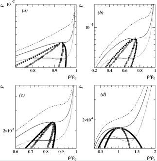
Figure 13: Thermodynamics of the Mekjian model [105], from [106]. Isotherms of pressure as a function of reduced density: (a) multifragmentation of charged nuclei with $A=162$; (b) as in (a) but with no Coulomb; (c) as (b) but with no temperature dependence of the surface free energies; (d) a van der Waals fluid. Full symbols show the coexistence zone, open symbols the spinodal zone. Solid curves correspond to the critical isotherm for each case: (a) $T_{C}=7.6$ MeV; (b) $T_{C}=6.9$ MeV; (c) $T_{C}=11.0$ MeV. Dotted and dashed curves are subcritical and supercritical, respectively.

Note that very recently predictions for new signatures of phase transition for hot nuclei to be confronted to data were proposed [107, 108, 109].

The thermodynamics of CTM/SMM were studied by Elliott and Hirsch [106], most notably the differences between charged or neutral matter, and the influence of the surface energy temperature dependence. Calculated pressure-density isotherms are presented in Fig. 13, and in all cases coexistence and spinodal regions can be identified up to some critical temperature. The effective critical temperature of the model does not correspond to the value of the parameter $T_{C}=16$ MeV used for the calculations; indeed even without such temperature dependence of the surface energy (Fig. 13(c)) there is still a coexistence region delimited by a critical isotherm. The effect of Coulomb on the critical temperature is surprisingly small, of the order of 10%.

The density range covered by the coexistence and spinodal regions changes most strongly according to the ingredients of the model. With the standard Coulomb and surface energy terms (Fig. 13(a)) the coexistence densities are surprisingly high, between 0.7 and 0.95$\rho_{0}$, much higher than could be realized with a closest packing of normal density nuclei as supposed in SMM and significantly higher than those typically used to compare model predictions to data. With Coulomb switched off (Fig 13(b)) the densities are more like those predicted by models for (neutral) nuclear matter, of the order of $0.35-0.75\rho_{0}$.

To conclude one can also note that using a classification scheme for phase transitions in finite systems based on the Lee-Yang zeros in the complex temperature plane [110, 111], it was shown that for this statistical model of nuclear multifragmentation the predicted phase transition is of first-order [112].

Microcanonical models (MMMC and MMM)

Historically, following the pioneering work of Randrup and Koonin [73], the Berlin group developed a microcanonical model [113, 114, 74] to better understand mass distribution of fragments for hadron-nucleus collisions at relativistic energies. In this rather simplified model the system of fragments is assumed to be stochastically expanded to a freeze-out volume of 6$V_{0}$; the reason for this choice comes from the difficulty to position the fragments in a smaller volume without overlapping and consequently demanding a lot of CPU time. The model only allows for sequential neutron evaporation from fragments. And no a priori hypothesis is made concerning the internal energies of excited fragments at freeze-out. This means that the vanishing of the level density, which is expected to occur at high excitation energies is not taken into account. As a consequence no limiting temperature for fragments is introduced [81]. This model which is known as Microcanonical Metropolis Monte Carlo - MMMC illuminated qualitatively various aspects of phase transition for hot nuclei. A more complete model called Microcanonical Multifragmentation Model - MMM was developed ten years later.

Within a microcanonical ensemble, the statistical weight of a configuration $C$, defined by the mass, charge and internal excitation energy of each of the constituting $M_{C}$ fragments, can be written as

$$W_{C}(A,Z,E,V)=\frac{1}{M_{C}!}\chi V^{M_{C}}\prod_{n=1}^{M_{C}}\left(\frac{\rho_{n}(\epsilon_{n})}{h^{3}}(mA_{n})^{3/2}\right)$$

$$\times~{}\frac{2\pi}{\Gamma(3/2(M_{C}-2))}~{}\frac{1}{\sqrt{({\rm det}I})}~{}\frac{(2\pi K)^{3/2M_{C}-4}}{(mA)^{3/2}},$$ (9)

where $A$, $Z$, $E$ and $V$ are respectively the mass number, the atomic number, the excitation energy and the freeze-out volume of the system. $E$ is used up in fragment formation, fragment internal excitation, fragment-fragment Coulomb interaction and kinetic energy $K$. $I$ is the inertial tensor of the system whereas $\chi V^{M_{C}}$ stands for the free volume or, equivalently, accounts for inter-fragment interaction in the hard-core idealization.

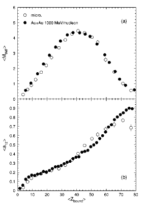
Figure 14: Fragment multiplicity (top panel) and charge asymmetry of the two heaviest fragments (bottom panel) of projectile spectators produced in ¹⁹⁷Au+¹⁹⁷Au collisions at 1000 MeV per nucleon incident energy. Full points refer to data and open points to MMM model. From [115].

In MMM [80] the statistical weights of each configuration and consequently the mean value of any global observables can be expressed analytically. Since the resulting formulas are not tractable, a statistical method is proposed. The method, which is a generalization of Koonin and Randrup’s procedure [81], provides an exploration of configuration space according to the detailed balance principle. This method is then applied to describe the phenomenon of multifragmentation. To obtain a realistic simulation, real binding energies of all the elements with $A$ lying between 1 and 266 are used. Calculated level densities include the excitation energy so as to describe the dependence of the factor entering the Fermi-gas formula for the ($A,Z$) nucleus with the binding energy $B$($A,Z$), limiting then temperature for fragments. The freeze-out density or volume is the only fitting parameter of the simulation. The model was then refined [115] by taking into account the experimental discrete levels for fragments with $A<7$ and by including the stage of sequential decays of primary excited fragments, thus allowing quantitative comparisons with data. As for SMM, radial expansion energies, fully decoupled from thermal properties, were also added for a better comparison with experiments.

Fig. 14 shows a comparison with data for projectile spectators produced in ¹⁹⁷Au+¹⁹⁷Au collisions at 1000 MeV per nucleon incident energy, which was used to deduce the sequence of excitation energy as a function of the projectile spectator $E^{*}(A)$. $M_{IMF}$ is the multiplicity of fragments (2$<$ Z $<$31). $a_{12}$ is the charge asymmetry of the two largests fragments $a_{12}$ = ($Z_{max}-Z_{2}$)/($Z_{max}+Z_{2}$) where $Z_{max}$ is the heaviest fragment and $Z_{2}$ is the second heaviest fragment. $Z_{bound}$ represents the charge bound in fragments.

Nuclear multifragmentation: comparison of different statistical ensembles

The sensitivity of different ensembles to the underlying statistical assumptions is a relevant information. Such a study was investigated in [116] by comparing microcanonical, canonical and canonical isobaric formulations within the SMM model. The work was carried out for the nuclear system $A$=168 and $Z$=75. The same break-up temperature is used in both canonical calculations and the break-up volume 3$V_{0}$ is the same for both microcanonical and canonical ensembles. The one for which the break-up volume is determined for each fragmentation mode is labelled “M.D. microcanonical” (Multiplicity Dependent) to distinguish it from the standard microcanonical version. The pressure, for the isobaric ensemble, was fixed at P = 0.114 MeV/fm³. The energy input used for the microcanonical ensemble was the average excitation energy obtained in the isobaric ensemble. We refer to [116] for more details. The main conclusions are the following: the microcanonical, canonical and isobaric implementations predict very similar average physical observables. Fig. 15 shows one example that concerns the evolution of the average break-up volume as a function of the thermal excitation energy: volumes obtained with the canonical isobaric and the M.D. microcanonical implementations are very similar, which indicates that the ad hoc multiplicity dependence of SMM is relevant.

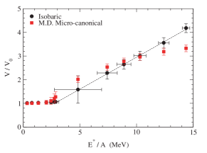
Figure 15: Average break-up (freeze-out) volume as a function of the excitation energy per nucleon predicted by the canonical isobaric and the Multiplicity Dependent microcanonical ensemble. Dashed line emphasizes the fairly linear dependence of the break-up volume on the excitation energy in the canonical isobaric ensemble. From [116].

4.3 Dynamical models

Beside statistical descriptions, there are microscopic frameworks that directly treat the dynamics of colliding nuclei such as the family of semi-classical simulations based on the nuclear Boltzmann equation (the Vlasov-Uehling-Uhlenbeck (VUU), Landau-Vlasov (LV), Boltzmann-Uehling-Uhlenbeck (BUU) or Boltzmann-Nordheim-Vlasov (BNV) codes [117, 118, 119, 120]), classical molecular dynamics (CMD) [121, 122, 123, 124], quantum molecular dynamics (QMD) [125, 126, 127], fermionic molecular dynamics (FMD) [128], antisymmetrized molecular dynamics (AMD) [129, 130, 131] and stochastic mean field approaches related to simulations of the Boltzmann-Langevin equation  [132, 133, 134, 135, 136, 137]. Boltzmann type simulations follow the time evolution of the one body density. Neglecting higher than residual two-body correlations, they ignore fluctuations around the main trajectory of the system (deterministic description), which becomes a severe drawback if one wants to describe processes involving instabilities, bifurcations or chaos expected to occur during the multifragmentation process. Such approaches are only appropriate during the first stages of nuclear collisions, when the system is hot and possibly compressed and then expands to reach a uniform low density. They become inadequate to correctly treat the fragment formation, and for the description of multifragmentation it is essential to include higher order correlations and fluctuations. This is done in molecular dynamics methods and in stochastic mean field approaches.

4.3.1 Quantum molecular dynamics: QMD and AMD simulations

QMD is essentially a quantal extension of the molecular dynamics approach widely used in chemistry and astrophysics. Starting from the n-body Schrödinger equation, the time evolution equation for the Wigner transform of the n-body density matrix is derived. Several approximations are made. QMD employs a product state of single-particle states where only the mean positions and momenta are time-dependent. The width is fixed and is the same for all wave packets. The resulting equations of motion are classical. Also the interpretation of mean position and momenta is purely classical and the particles are considered distinguishable; this simplifies the collision term which acts as a random force. All QMD versions use a collision term with Pauli blocking in addition to the classical dynamics. Some versions consider spin and isospin and others do not distinguish between protons and neutrons (all nucleons carry an average charge). As with most dynamical models a statistical decay code must be coupled to describe the long time evolution (called an after-burner). However for the code of Ref. [126] there is no need to supplement the QMD calculations by an additional evaporation model [138]. It is important to emphasize here that QMD codes are certainly better adapted for the higher incident energies.

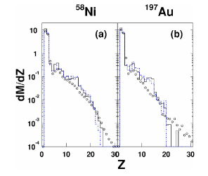
Figure 16: Charge distribution of fragments produced in central collisions for ⁶⁴Zn on (a) ⁶⁸Ni and on (b) ¹⁹⁷Au at 47 MeV per nucleon incident energy. Experimental results are shown by circles and calculated results (AMD-V) correspond to dot-dashed lines (soft EOS) and to solid lines (stiff EOS). From [139].

An antisymmetrized version of molecular dynamics (AMD) was constructed by incorporating the two-nucleon collision process as the residual interaction into the fermionic molecular dynamics (FMD). AMD describes the system with a Slater determinant of Gaussian wave packets and therefore can describe quantum-mechanical features. However, in the dynamics of nuclear reactions, there may be other phenomena caused by the wave packet tail that are completely lost in AMD due to the restriction of the single-particle states. So an improvement was realized (called AMD-V) with the stochastic incorporation of the diffusion and the deformation of wave packets which is calculated by the Vlasov equation without any restriction on the one-body distribution [130]. After that the quantum branching process due to the wave packet diffusion effect was treated as a random term in a Langevin-type equation of motion whose numerical treatment is much easier. Moreover a new approximation formula was also introduced in order to evaluate the Hamiltonian in the equation of motion with much less computation time than the exact calculation, so that systems like Au+Au became tractable [140]. More recently a method was proposed to allow the possibility to form particles of mass numbers $A$ = 2, 3 and 4. Details can be found in [141, 142]. As for most dynamical models the stiffness of the effective interaction and the in-medium nucleon-nucleon cross-section are both important ingredients for determining the degree of agreement with experimental data. In order to test the sensitivity of the ingredients, a detailed study of reaction dynamics and multifragmentation was made in Ref. [139] by comparing AMD-V calculations with data from heavy-ion reactions around the Fermi energy. Fig. 16 presents the charge distribution of reaction products from central collisions between ⁶⁴Zn projectiles and (a) ⁶⁸Ni and (b) ¹⁹⁷Au targets at 47 MeV per nucleon incident energy. Lines correspond to AMD-V results obtained with both stiff and soft EOS, which rather well agree with data. We refer the reader to Ref. [139] for more details.

4.3.2 Stochastic mean field approaches: SMF, BOB and BLOB simulations

The stochastic mean field models used are semi-classical nonrelativistic transport approaches. The time evolution of the nuclear system is described in terms of the one-body distribution, as ruled by the nuclear mean-field (plus Coulomb interaction for protons) and hard two-body scattering, according to the so-called Boltzmann-Langevin equation (BLE),

$$\partial f/\partial t=\{h[f],f\}+\overline{I}[f]+\delta I[f],$$ (10)

which was introduced for heavy-ion collisions in Ref. [132, 133, 134]. $f$ is the one-body phase space density. The first term on the r.h.s. produces the collisionless propagation of $f$ due to the self-consistent mean field described by the effective Hamiltonian. The second term, called collision term, represents the average effect of the residual Pauli-suppressed two-body collisions; this is the term included in LV, BUU and BNV simulations. The third term is the Langevin term which accounts for the fluctuating part of the two-body collisions. Exact numerical solutions of the BLE are very difficult to obtain and have only been calculated for schematic cases in one or two dimensions [143]. Therefore various approximate treatments of the BLE have been developed and the test-particle method is used to solve Eq. (10). Fluctuations are introduced within the mean field treatment according to various approaches.

In the Stochastic Mean Field Model SMF [144], fluctuations are produced by agitating the spatial density profile [145, 146]. Once local thermal equilibrium is reached, the density fluctuation amplitude $\sigma_{\rho}$ is evaluated by projecting on the coordinate space the kinetic equilibrium value of a Fermi gas. Then, in the cell of $\bm{r}$ space being considered, the density fluctuation $\partial\delta_{\rho}$ is selected randomly according to the Gaussian distribution exp($-\partial\delta_{\rho}^{2}$/2$\sigma_{\rho}^{2}$). This determines the variation of the number of particles contained in the cell. A few leftover particles are randomly distributed again to ensure conservation of mass. Momenta of all particles are finally slightly shifted to ensure momentum and energy conservation.

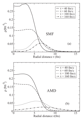
Figure 17: Density profiles at several times obtained in SMF (a) and AMD (b) models, for ¹¹²Sn + ¹¹²Sn central collisions (b = 0.5 fm) at 50 MeV per nucleon incident energy. From [147].

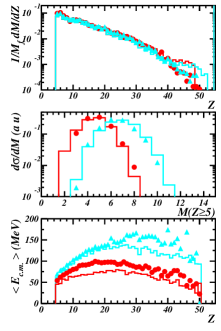
Figure 18: Comparison of experimental data (quasifusion from central collisions: Gd+U - 36 MeV per nucleon and Xe+Sn - 32 MeV per nucleon incident energies) with BOB simulations for charge and multiplicity distributions of fragments (top and middle panels) and for their average kinetic energies (bottom panel). The symbols are for data and the lines for BOB simulations. Light grey lines and triangles stand for Gd+U and black lines and circles for Xe+Sn. Adapted from [148].

A quantitative comparison of SMF and AMD models was made in [147, 42]. They both predict fragment formation leading to multifragmentation but with different mechanisms. For SMF, fragmentation is linked to the spinodal decomposition mechanism (i.e. to mean field instabilities) whereas in AMD, many-body correlations are sufficient to produce fragments. Fig. 17 shows the time evolution of the density profile for the two models and it concerns ¹¹²Sn + ¹¹²Sn central collisions (b = 0.5 fm) at 50 MeV per nucleon incident energy. The qualitative evolution of compression and expansion is similar but we notice that AMD shows broader average density distribution than SMF as the system expands, pointing to a faster expansion in AMD in which fragments have already appeared and are distributed widely in space. We notice that early fragment formation is observed for all models belonging to the class of molecular dynamics. To conclude on SMF we also report to the reader an exhaustive comparison of experimental data with SMF model in [43].

In many domains of physics a diffusive behaviour is described by transport theories which were originally developed for Brownian motion. The effects of the disregarded degrees of freedom are simulated by a random term in the dynamics of the retained variables. It is the basic idea of the Brownian One-Body dynamics model BOB [149]. The fluctuating term is replaced by

$$\delta\tilde{I}[f]=-\delta\bm{F}[f].\partial f/\partial\bm{p}$$

where $\delta\bm{F}(\bm{r},t)$ is the associated Brownian force ($<\delta\bm{F}>=0$). Since the resulting Brownian one-body dynamics mimics the BL evolution, the stochastic force is assumed to be local in space and time. The strength of the force is adjusted to reproduce the growth of the most unstable modes for infinite nuclear matter in the spinodal region (see 6.4). Quantal fluctuations connected with collisional memory effects are also taken into account as calculated in [150].
An extensive comparison data-BOB was made for two very heavy quasifusion systems produced in Xe+Sn and Gd+U central collisions which undergo multifragmentation with about the same excitation energy ($\sim$ 7 MeV per nucleon) [148, 151, 152]. Stochastic mean field simulations were performed for head-on collisions with a self-consistent mean field potential chosen to give a soft EOS (K_∞= 200 MeV). The finite range of the nuclear interaction was taken into account using a convolution with a Gaussian function with a width of 0.9 fm. A term proportional to $\Delta\rho$ in the mean-field potential was added; it allows to well reproduce the surface energy of ground-state nuclei, which is essential in order to correctly describe the expansion dynamics of the fused system. In the collision term a constant nucleon-nucleon cross-section value of 41 mb, without in-medium, energy, isospin or angle dependence was used. As a second step the spatial configuration of the primary fragments, with all their characteristics as given by BOB, was taken as input in a statistical code to follow the fragment deexcitation while preserving space-time correlations. Finally the events were filtered to account for the experimental device. These simulations well reproduce the observed charge and multiplicity distributions of fragments (see Fig. 18). Particularly experimentally observed independence of the charge distribution against the mass of the system was recovered [153]. More detailed comparisons of the charge distributions of the three heaviest fragments also show a good agreement [148]. Kinetic properties of fragments are rather well reproduced for the Gd+U system, whereas for Xe+Sn the calculated energies fall $\sim$ 20% below the measured values.

At this stage it is important to stress that both statistical (SMM) and dynamical (BOB) models are able to well reproduce experimental data; it is illustrated by Fig. 12 and Fig. 18 for quasifusion data from Xe+Sn at 32 MeV per nucleon incident energy. It may at first seem surprising that the results of a dynamical description are so close to those of a statistical model. As thermodynamic equilibrium corresponds to an unbiased population of the available phase space it is a strong indication that the dynamics (first governed for BOB by mean field instabilities) is effective in filling at least a large part of phase space. The mixing of a selected set of events also contributes to the large covering of phase space; it is also true for theoretical simulations due to fluctuations in the number of nucleon-nucleon collisions in the entrance channel.

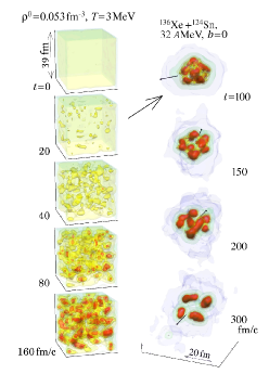
Figure 19: Density landscape at several times for nuclear matter in a periodic box (left panel) and for a hot nuclear system (right panel) formed in a head-on collision. Small arrows indicate the beam direction. For the big arrow see text. From [154].

Recently a numerical treatment of Eq. (10) in which fluctuations are introduced in full phase space from induced nucleon-nucleon collisions has been proposed (BLOB simulation) [154]. This transport simulation based on a complete treatment of the Boltzmann-Langevin approach proves to be very efficient in building fluctuations for equilibrated systems and preserving fluctuations of larger amplitudes, which leads to a more reliable description of the onset of multifragmentation. Fig 19 illustrates the correspondence between a portion of nuclear matter ($T$ = 3 MeV and $\rho\sim\rho_{0}/3$) and a hot nuclear system formed in a central collision between ¹³⁶Xe and ¹²⁴Sn at 32 MeV per nucleon incident energy. We observe some analogy (big arrow) between the early time when inhomogeneities emerge in nuclear matter (20 fm/c) and when fragments start forming in a nuclear system (around 100 fm/c) after accessing low-density spinodal conditions. In both systems, a spinodal signal stands out by exhibiting equal-size inhomogeneities in configuration space within a similar timescale [155] and it is smeared out later on (see 6.4).

To conclude on dynamical descriptions of multifragmentation and fragment formation, one can make a few general comments. For AMD and stochastic mean-field simulations at incident energies around 35-50 MeV per nucleon a maximum density of 1.2-1.6 $\rho_{0}$ is observed at 30-40 fm/$c$ after the beginning of central heavy-ion collisions and the normal density is recovered around 60 fm/c. Thermal equilibrium times are found in the range 100-140 fm/c after the beginning of collisions, well before freeze-out configurations (200-300 fm/$c$). Primary fragments exhibit an equal or almost equal excitation energy per nucleon of 3-4 MeV in good agreement with values deduced from experiments [156, 157]. The mechanism of fragment production differs depending on model type. In molecular dynamics models fragments are preformed at early stages close to the normal nuclear density whereas in stochastic mean field calculations fragment formation is linked to spinodal instabilities; mononuclear systems at low density ($\sim$0.4$\rho_{0}$) formed at around 100 fm/$c$ develop density fluctuations during about 100 fm/$c$ to form fragments. More constrained observables related to the formation of fragments by spinodal instabilities will be discussed in 6.4. As a last point, dynamical calculations exhibit radial collective energies for fragments with average values in the range 0.1-2.0 MeV per nucleon for heavy-ion collisions in the Fermi energy domain which agree fairly well with values derived from experiments (see [13]).

4.4 Information on thermodynamic variables

Excitation energy can be derived from experiments through calorimetry with some precautions. Indeed the formed multifragmenting hot nuclei/nuclear systems are accompanied by preequilibrium emission produced mainly by first and second chance nucleon-nucleon collisions. These early emitted particles, mostly neutrons, $H$ and $He$, must not be included in the calculation of the mass and of the excitation energy of the fragmenting system. In experimental analyses, preequilibrium particles are excluded either through angular and energetic properties of the observed products [148] or with the help of models. For thermal energy, as mentioned before, the collective energy to remove (generally a small part of total excitation energy) is evaluated from models constrained by experimental data. As far as temperature is concerned several methods have been proposed and applied. However substantial differences between thermometers have been observed when the excitation energy or incident energy increases, which seems to indicate that thermometers are not always measuring the same thing. We will shortly discuss this problem. It is why temperature is often deduced from a statistical model that well reproduces the data.

4.4.1 Calorimetry

All procedures for obtaining the excitation energy of a fragmenting source, observed with a 4$\pi$ array, are based on the determination of its velocity. For central collisions the reaction centre of mass velocity is most often chosen whereas the quasi-projectile and the projectile spectator velocities are either identified with that of the biggest fragment, or with that of the subsystem containing all the fragments (Z$\geq$3 or 5), forward emitted in the centre of mass. The excitation energy, $E^{*}$, of the source is then calculated event by event with the relation $E^{*}=\sum_{M_{cp}}E_{cp}+\sum_{M_{n}}E_{n}-Q$. $E_{cp}$ and $E_{n}$ are respectively the kinetic energies of charged products and neutrons emitted by the source, $Q$ is the mass difference between the source and all final products. Energies are expressed in the source reference frame. $M_{cp}$ is in most cases the detected multiplicity of charged products. The energy removed by gamma rays is small and most often neglected in the calculation. The way in which different charged products are attributed to the sources differs with the experimental apparatus and the type of collision under study. For central symmetric heavy-ion collisions, all fragments with Z$\geq$3 (or 5) are attributed to the source. Preequilibrium in that case is mostly forward/backward emitted, and indeed the angular distributions of the light products appear isotropic between 60 and 120^o. The charge, mass and energy contributions of these particles are doubled for the calculation of the characteristics of the source (i). Another possibility, to account for the detector inefficiency, is to calculate the charge, mass and energy of the anisotropic part, and to remove it from those of the composite system (ii). For quasi-projectiles the most important contamination comes from mid-rapidity products and several techniques are used for the quasi-projectile reconstruction. i) All fragments forward emitted in the reaction c.m. system are attributed to the quasi-projectile. Variants consist either in putting a low velocity cut for the lighter fragments [158, 159], or in keeping only events with a compact fragment configuration in velocity space [160, 87]. Then twice the light elements in the quasi-projectile forward hemisphere are added. ii) Fragments are treated as above, but particles are attributed a probability to come from the quasi-projectile emission, either using a 3-source fit [161], or by taking a well characterized subspace as reference [162, 163]. The velocity of the quasi-projectile is then recalculated by including all its components. For projectile spectators, the highest energy deposits are obtained with an intranuclear cascade model [164]. They represent the sum of the hole energies left behind by nucleons knocked-out from the spectator and of the energies carried by struck nucleons captured into the spectator. The projectile spectator reconstruction is generally made including the measured abundances for Z $\geq$ 2 and the yields of hydrogen isotopes are deduced by extrapolating to Z = 1 whereas free neutrons are usually measured [165, 166]. Finally in hadron-induced collisions, products emitted from the source are chosen from energetic considerations, by excluding those with an energy per nucleon above a given threshold either fixed [167] or varying with Z [12]. All those procedures assume forward-backward symmetry of particle emission in the source frame. For quasi-projectiles the symmetry of the source emission may be questionable when highly excited quasi-projectiles and quasi-targets start emitting right after their separation [168, 169]: the close proximity of the partner deforms phase space and emission is favoured between quasiprojectile and quasitarget. This possible effect is generally ignored.

Once all charged products have been attributed to the source, its charge is known. A first uncertainty is introduced in calculating the mass of the source in the cases where the masses of all associated decay products (especially heavy fragments) are not measured. A single mass can be attributed to all nuclei with a given atomic number, either that of the most stable species, or that derived from formulae existing in the literature (EPAX [170] or EAL [171]). At that point neutrons must be included. Except in experiments using a neutron ball or a neutron wall in experiments with relativistic spectators, neither their multiplicity not their energy is known. The neutron number can then be estimated by assuming that the source has the same N/Z ratio as the total system (central or hadron-induced collisions) or as the projectile. The average neutron energy is then taken equal to the proton energy averaged over the event sample after subtraction of some estimate of the Coulomb barrier. Note that with neutron balls only the neutron multiplicity is measured, at the price of a poor geometrical coverage for charged products. In that case corrections accounting for the undetected particles and neutrons are made [172].

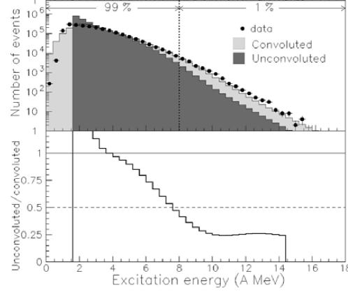
Figure 20: Top : Convoluted, unconvoluted and experimental excitation energy distributions obtained in $\pi$+Au reactions. Bottom : Ratio of unconvoluted-to-convoluted distribution as a function of the excitation energy per nucleon. Adapted from [173]

In central heavy-ion reactions, the populated excitation energy domain is narrow: $\sigma_{E^{*}}\sim$ 0.7 - 1.25 MeV per nucleon; the width includes experimental effects (detector efficiency and resolution), calculation assumptions and physical effects (pre-equilibrium). Conversely, in hadron-induced reactions as well as in quasi-projectile and projectile spectator studies, a broad domain of excitation energy is populated, proportionally to the partial cross section, function of the impact parameter. However, due to on-line trigger effects very low energies are poorly sampled, for example due to the acquisition trigger based on a minimum multiplicity of charged products; indeed neutron emission - often not detected or with low efficiencies - is dominant in this region. At the other end of the distribution, the very high energies probably result from significant fluctuations. In all cases the reliable domain extends from about 2 to 8 MeV per nucleon: for example in Fig. 20 obtained in $\pi$+Au reactions, the excitation energy distribution is unconvoluted assuming Gaussian fluctuations. More than half of the 1% of events above the vertical dotted line have an energy overestimated by 1-2 MeV per nucleon [173].

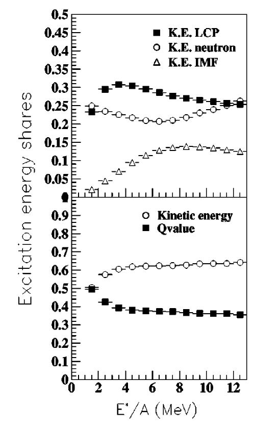
Figure 21: Relative share of excitation energy for various components of the reconstruction procedure as a function of the excitation energy per nucleon. From [173]

How reliable are the energies so obtained ? Because of compensation of the errors on the mass and on the energy, the excitation energy per nucleon is a more robust experimental observable than the total excitation energy. By comparing values obtained by different methods for quasi-projectiles, differences on $E^{*}/A$ smaller than 10% were found [174, 87]. From simulations with an event generator, the reconstructed values were found to differ from the true values by less than 10%, except for very peripheral collisions where the discrepancies are much larger [162]. In central collisions, excitation energies slightly smaller than the available energies are generally found, which is what can reasonably be expected. It was verified in the INDRA Xe+Sn data that the two procedures for central collisions give the same results when a high degree of completeness is required, e.g. that at least 90% of the system charge be measured for each event in the considered sample. For lesser completeness (80%), the difference between both types of calculation increases with the incident energy, reaching 1 MeV per nucleon (10%) at 50 MeV per nucleon incident energy. The main source of uncertainty in the calculation of $E^{*}$ comes from the neutron terms. However, compensation occurs in the calorimetry equation between the kinetic and the mass balance terms; indeed the weight of these two terms is similar for quasi-projectiles and in hadron-induced reactions ($Q/E^{*}\sim$30-36% [173, 175] - see Fig. 21); in central collisions the $Q$ term accounts for only $\sim$20% of the excitation energy.

4.4.2 Temperature measurements

Two reviews extensively describe the methods most used for temperature measurements ([176, 177] and references therein). A brief summary will be given here. We will also draw attention to the inconsistency of temperature measurements when using different thermometers. The concept of temperature for a nucleus, which is a microscopic, isolated Fermionic charged system, is not a priori obvious. However we recall following our previous discussions (see section 3.2) that the intensive variables such as temperature can always be defined for statistical ensembles constructed from homogeneous samples of selected hot nuclei. As no probe can be used to measure the temperature of these small systems, it has to be derived from the properties of particles that they emit during their cooling phase. Three families of methods are used to ”measure” temperatures.

1. Kinetic temperatures. Historically, temperatures of compound nuclei were derived from the slopes of the kinetic energy spectra of the emitted neutrons or charged particles that they evaporate, as the spectra can be fitted with Maxwell-Boltzmann distributions [71] (see Fig. 25). At higher energies, when long chains of particles are emitted, the obtained result is an average over the deexcitation chain, and may differ from one particle to another, depending on the emission sequence. To retrieve the initial temperature, it was proposed to subtract from the spectra those of particles coming from the same nucleus formed at lower excitation energies [178]. For multifragmenting systems, the slopes of light product spectra lead to very high ”temperatures”, and probably do not reflect only the thermal properties of the system, but also the collective energies coming from the dynamics of collisions.

2. Excited state temperature. Thermometers are based upon the relative populations of excited states of emitted particles. The underlying idea for this method is that the population of the excited states of a system in statistical equilibrium is given by the temperature of the system and the energy spacing, $\Delta E$ = $E_{1}$ - $E_{2}$, between the levels.

   $$T=\frac{E_{1}-E_{2}}{ln(a^{\prime}Y_{1}/Y_{2})}$$ (11)

   Here $a^{\prime}=(2J_{2}+1)/(2J_{1}+1)$, $E_{i}$ the excitation energy, $Y_{i}$ is the measured yield and $J_{i}$ is the spin of the state $i$. This definition in itself bears the limits of the method: when the temperature is higher than $\Delta E$, the ratio between the population of two states saturates. Considering particle-unbound states is thus interesting as it allows to measure higher temperatures, and the population ratio should in that case be less influenced by secondary decays. Anyhow the considered emitted particles should be present at freeze-out.

   

   

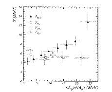
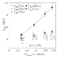
   Figure 22: Measured isotope temperatures and excited state temperatures; (left) as a function of the experimental excitation energy per nucleon for target spectators produced in Au on Au collisions at 1GeV per nucleon incident energy; (right) as a function of incident energy for central collisions between Kr and Nb. From [166] and adapted from [179].

3. Isotope temperature. This method uses the yields of different light isotopes produced by the system. It was developed in the grandcanonical approach, and is valid for systems at densities low enough to make fragment nuclear interaction negligible, thus the chemical composition of the system is frozen [180]. The basic assumption is that free nucleons and fragments are in thermal equilibrium within an interaction volume V. The density of an isotope reads: $\rho(A,Z)=N(A,Z)/V=A^{3/2}\omega(A,Z)\lambda_{T_{N}}^{-3}\exp(\mu(A,Z)/T)$, where $\omega$ is the internal partition function of particle ($A,Z$), $\mu$ its chemical potential and $\lambda$ the thermal nucleon wavelength. The condition of chemical equilibrium allows to define the chemical potential of a species in terms of those of free neutrons and protons and of its binding energy. Using two sets of two nuclei differing only by one nucleon, the temperature is derived from the double yield ratio, the binding energy differences $B$ and the partition functions only, the other terms disappear.

   $$T=\frac{B}{ln(a(Y_{1}/Y_{2})/(Y_{3}/Y_{4}))}$$ (12)

   where $Y_{1}$, $Y_{2}$ are the yields of one isotope pair and $Y_{3}$, $Y_{4}$ is another isotope pair; $a$ contains the statistical weighting factor. A first problem lies in the calculation of the binding energies which might depend on density and temperature. Different corrections were proposed to account for finite-size effects [181] or secondary decays [182, 183]. But again this equation assumes that the considered particles should be present at freeze-out, and not produced by secondary decays.

This last point which appears for both thermometers can explain why they can give different temperatures. This is well illustrated by Fig. 22. Temperatures have been extracted from very different experiments; for central Kr + Nb collisions (right) one can roughly convert the beam energy scale saying that 50 MeV per nucleon corresponds to 10 MeV per nucleon excitation energy. The same trend is observed on both figures: the HeLi isotope temperature differs from other measurements above around 10 MeV per nucleon excitation energy. Without entering here in a deep discussion, it appears a posteriori that the HeLi isotope temperature seems closer to the real temperature above 10 MeV per nucleon excitation energy.

More recently another method for measuring the temperature of hot nuclei was proposed [184, 185]. It is based on momentum fluctuations of emitted particles, like protons, in the centre of mass frame of the fragmenting nuclei. In a classical picture, assuming a Maxwell-Boltzmann distribution of the momentum yields, the temperature $T$ is deduced from the quadrupole momentum fluctuations defined in a direction transverse to the beam axis:
$\sigma^{2}$ = $<Q_{xy}^{2}>$ - $<Q_{xy}>^{2}$ = $4m^{2}T^{2}$
with $Q_{xy}$ = $p_{x}^{2}$ - $p_{y}^{2}$; $m$ and $p$ are the mass and linear momentum of emitted particles. If we now take into account the quantum nature of particles, a correction $F_{QC}$ related to a Fermi-Dirac distribution was also proposed [185, 186].
In that case $\sigma^{2}$ = $4m^{2}T^{2}$ $F_{QC}$ where $F_{QC}$ = $0.2(T/\epsilon_{f})^{-1.71}$ + 1;
$\epsilon_{f}$ = 36 $(\rho/\rho_{0})^{2/3}$ is the Fermi energy of nuclear matter at density $\rho$ and $\rho_{0}$ corresponds to saturation density. Density can be estimated from models. Again this method can be useful for relevant measurements by selecting particles emitted at freeze-out.

To conclude, one can say that direct temperature measurements are questionable and we will see that, very often, temperatures are derived from comparisons of data to statistical models or from simulations starting from data and able to recover with a good level of confidence freeze-out properties.

4.4.3 Break-up densities and freeze-out volumes

No sufficiently accurate method is available to determine precisely the spatial extension of hot nuclei/nuclear systems which undergo multifragmentation. However we will see that derived estimates are rather coherent despite the variety of methods used; three examples are chosen to illustrate those determinations.

Break-up densities for projectile spectator fragmentation in ¹⁹⁷Au+¹⁹⁷Au collisions at 1000 MeV per nucleon incident energy were estimated by using selected particle-particle correlations (particles from secondary decays are excluded by imposing an energy threshold) [187]. Assuming zero lifetime, the volumes of spectator sources were extracted and densities calculated by dividing the number of spectator constituents by the source volume. The estimated average values slowly decrease from about 0.4 to 0.2 $\rho_{0}$ when excitation energies of spectators increase from 4 to 10 MeV per nucleon.

The average freeze-out volume can also be experimentally estimated from the mean detected fragment kinetic energy ($<E_{kin}>$). Concerning quasi-projectile data (¹⁹⁷Au+¹⁹⁷Au mid-peripheral collisions at 35 MeV per nucleon incident energy [188]), after subtracting a small contribution of collective energy (i.e. non thermal and non-Coulomb), a many-body Coulomb trajectory calculation can be performed by randomly placing the reconstructed primary fragments in a spherical volume and letting them evolve in the Coulomb field. Under the reasonable hypothesis that, on average, particles evaporated from fragments do not affect fragment velocities, the superposition of the average Coulomb and thermal motions provides an observable directly comparable to $<E_{kin}>$ data corrected from collective energies. This comparison allows to estimate directly from data a range of freeze-out volumes. The result is displayed in Fig. 23. The full lines, which better agree with data, correspond to volumes of 3$V_{0}$ on average. Note that the hypothesis of cold fragments (Fig. 23 - bottom part), which is very extreme, gives an idea of the sensitivity of the method.

Figure 23: Average fragment kinetic energy (corrected from collective energy) as a function of the thermal excitation energy for quasi-projectiles produced in ¹⁹⁷Au+¹⁹⁷Au mid-peripheral collisions at 35 MeV per nucleon incident energy. Full points are corrected data and bars represent the statistical errors. Lines correspond to mean many-body trajectory calculations for a volume of 3$V_{0}$ (full), 4$V_{0}$ (dotted), 5$V_{0}$ (dashed dotted) and 6$V_{0}$ (long dashed). The bottom part refers to an extreme unphysical case. From [188].

Another possibility is to make a simulation for estimating the freeze-out properties in a fully consistent way. Such a simulation was done for quasifusion hot nuclei produced in Xe+Sn central collisions between 32 and 50 MeV per nucleon incident energy [189, 157]. The method for reconstructing freeze-out properties requires data with a very high degree of completeness (measured fraction of the total available charge $\geq$93% in this study), crucial for a good estimate of Coulomb energy. Quasifusion nuclei are reconstructed, event by event, from all the available asymptotic experimental information (charged particle spectra, average and standard deviation of fragment velocity spectra and calorimetry). Dressed excited fragments, which statistically deexcite, and particles at freeze-out are described by spheres at normal density. Four free parameters are used to recover the data: the percentage of measured particles which were evaporated from primary fragments, the collective radial energy, a minimum distance between the surfaces of products at freeze-out and a limiting temperature for fragments which was mandatory to reproduce the observed widths of fragment velocity spectra (see [157] for details). The agreement between experimental and simulated velocity/energy spectra for fragments, for the different beam energies, is quite remarkable (see Fig. 3 of [157]). Relative velocities between fragment pairs were also compared through reduced relative velocity correlation functions [190, 152] (see Fig. 4 of [157]). Again a good agreement is obtained between experimental data and simulations, which indicates that the retained method (freeze-out topology built up at random) and the deduced parameters are sufficiently relevant to correctly describe the freeze-out configurations, including volumes. Volumes were estimated from an envelope of all the nuclei. The average values evolve from 3.9 to 5.7$V_{0}$ between 32 and 50 MeV per nucleon incident energy whereas average thermal excitation energies of quasifusion nuclei increase from 5.7 to 9.6 MeV per nucleon. A comparison with the results of a microcanonical statistical model (MMM) was also performed to verify the overall physical coherence of the built simulation [157].

In conclusion we can say that working hypotheses and approximations are used to give semi-quantitative information on average break-up densities or freeze-out volumes. At large excitation energy, around 10 MeV per nucleon, rather constant values around 0.2$\rho_{0}$ (5-6$V_{0}$) are found whereas values from 0.2 to 0.4$\rho_{0}$ are derived at lower excitation energies.

5 Two well-identified phases

Before discussing LG type phase transition signatures for hot nuclei, we will recall some aspects of liquidlike behaviour of nuclei in their ground states or at low excitation energies and characterize their vaporization at very high excitation energies.

5.1 Liquid aspects of nuclei: binding energy, fission and evaporation

For many purposes the nucleus can be viewed as a charged liquid drop. Three examples are chosen to illustrate this vision of nuclei: the liquid drop model, the fission shapes and the definition of the fissility parameter and the particle evaporation from excited nuclei.

In the liquid drop model the nucleus is viewed as a charged spherical liquid drop [191, 192]. In such a model, one would expect the nuclear binding energy to be expressed as a bulk or volume term due to the attractive force between nucleons, a surface correction due to the fact that surface nucleons are surrounded on average by a smaller number of nucleons, a second negative contribution due to repulsive Coulomb forces between protons and a third one produced by an excess of protons or neutrons. Thus

$$B(N,Z)=a_{V}A-a_{S}A^{2/3}-a_{C}\frac{Z^{2}}{A^{1/3}}-a_{A}\frac{(N-Z)^{2}}{A}$$ (13)

where successive terms represent respectively bulk, surface, Coulomb (Coulomb energy of a charged sphere) and asymmetry contributions. The parameter related to the symmetry energy of finite nuclei at saturation density (see also 2.1.2) was deduced using formula (13) in [193] from a fit to over 3100 nuclei with mass number $A>10$ and gives $a_{A}$ = 22.5 MeV. In this idealization of the nucleus no account is taken of shell effects or residual interactions arising from independent particle motion in the nucleus.

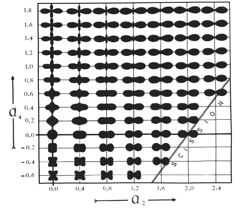
Figure 24: Liquid drop shapes corresponding to various locations on an $\alpha_{2}$-$\alpha_{4}$ map. The figures possess rotational symmetry about the horizontal axis. From [194].

Considering fission, in order to accurately describe distorsions of a sphere as large as are encountered at the top of the fission barrier, or saddle point, it is convenient to describe the drop shape in terms of an expansion in Legendre polynomials:

$$R(\theta)=(R_{0}/\lambda)[1+\sum_{n}\alpha_{n}P_{n}(cos\theta)].$$ (14)

The parameter $\lambda$ is a scale factor required to ensure that the volume remains constant at the value for the sphere of radius $R_{0}$. Shapes associated with different combinations of the leading coefficients $\alpha_{2}$ and $\alpha_{4}$ are given in Fig. 24. The surface and Coulomb energies for small distorsions are given by [195] $E_{S}=E_{S}^{0}(1+2/5\alpha_{2}^{2})$ and $E_{C}=E_{C}^{0}(1-1/5\alpha_{2}^{2})$ where $E_{S}^{0}$ and $E_{C}^{0}$ are the surface and Coulomb energies of undistorted spheres. In order for the charged liquid drop to be stable against small distortions, the decrease of Coulomb energy (-1/5$\alpha_{2}^{2})E_{C}^{0}$ must be smaller than the increase in surface energy (2/5$\alpha_{2}^{2})E_{S}^{0}$. The drop will become unstable when $E_{C}^{0}$/$E_{S}^{0}$ = 1. Following Bohr and Wheeler [195] the fissility parameter $x$ is defined to be equal to this ratio $x$ = $E_{C}^{0}$/$E_{S}^{0}$.

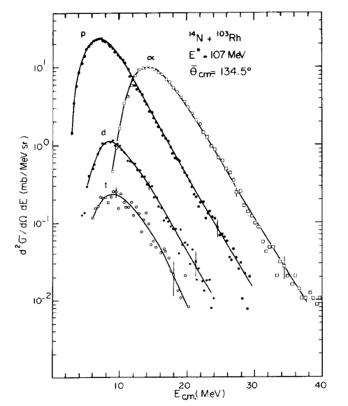
Figure 25: Evaporated charged particle spectra emitted from the ¹¹⁷Te compound nucleus formed around 1 MeV per nucleon excitation energy. From [196].

For particle evaporation, the behaviour of nuclei at excitation energies around 1 MeV per nucleon has been extensively studied and rather well understood using statistical models [71, 197, 198]. At these energies there is a clear separation of the timescales between compound nucleus formation, equilibration and subsequent decay (see section 3.2). The theoretical treatment of particle emission involves the estimation of microstate densities defined for equilibrium states. Excited nuclei are formed in fusion reactions below around 5 MeV per nucleon incident energies, which produce a well-defined set of events and the canonical ensemble (fixed number of particles) is the best suited to study deexcitation energy properties. At such excitation energies the density stays very close to normal density of cold nuclear matter and the earliest evaporation model rests on the basic idea: an emitted particle can be considered as originally situated somewhere on the surface of the emitting nuclei at a given temperature and with a randomly directed velocity, it is why we use the term evaporation. Moreover particles are emitted sequentially and independently without any correlation. Fig. 25 illustrates through Maxwellian spectra for protons, deuterons, tritons and alpha-particles the evaporation process. Note the similar high energy slope for all particles which indicates a given temperature.

5.2 Gas phase: onset and characterization

First indications of excitation energy needed to enter the gas phase were obtained from combined (and independent) determinations of thermal excitation energy and of estimated temperatures of hot nuclei. On the theoretical side, caloric curves were estimated using the Monte Carlo method in a thermodynamical model based on a finite-temperature liquid-drop description of nuclear properties and a related canonical approximation [199]. Fig. 27 shows that at excitation energies above around 10 MeV per nucleon the system behaves like a free gas if nuclei are heavier than around $A$ = 50. Experimentally, the first caloric curve was derived by the ALADIN collaboration from a study of fragment distributions resulting from projectile spectators produced in Au+Au collisions at 600 MeV per nucleon incident energy. Excitation energies per nucleon of primary fragments were determined from the measured fragment and neutron distributions and temperatures estimated from yield ratios of He and Li isotopes [165].

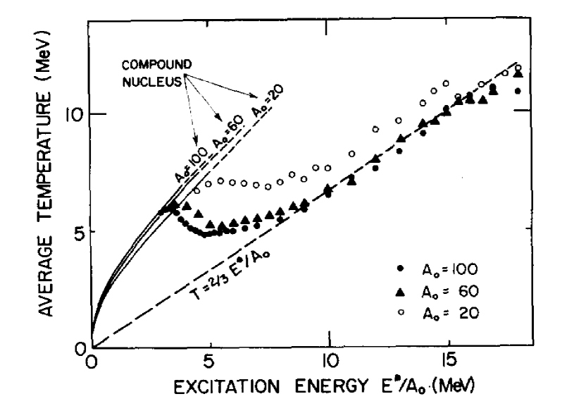
Figure 26: Mean temperature $T$ as a function of the excitation energy per nucleon for three different masses of nuclei. The dashed line gives the free gas limit. From [199].

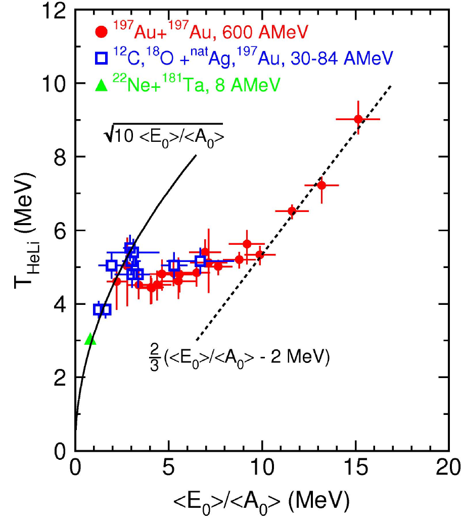
Figure 27: Caloric curve of nuclei determined by the dependence of the isotope temperature on the excitation energy per nucleon (see text). From [165].

Fig. 27 shows the isotope temperature as a function of the total excitation energy per nucleon. Data for target residues produced at lower incident energies between 30 and 84 MeV per nucleon are also shown (open squares) together with one value below 2 MeV per nucleon excitation energy provided by Ne+Ta fusion reaction at 8.1 MeV per nucleon incident energy (triangle). Again, beyond an excitation energy of 10 MeV per nucleon, a steady rise of temperature with increasing excitation energy is observed with a slope which alludes to a free gas; the offset of 2 MeV was interpreted as indicating a freeze-out density around 0.15 - 0.3$\rho_{0}$.

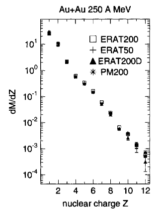
Figure 28: Measured multiplicities of vaporized events produced in central collisions as function of nuclear charge for various central event selections. From [200].

As theoretically predicted the nuclear gas phase is not only composed of single nucleons, protons and neutrons. It was observed by the FOPI collaboration studying central ¹⁹⁷Au+¹⁹⁷Au collisions in the beam energy range 150 - 400 MeV per nucleon [200]. Fig. 28 displays the composition of the pure gas phase obtained at 250 MeV per nucleon incident energy for charged products: we observe light nuclei up to Mg. The measured complete composition is the following: 45.3% of neutrons, 51.2% of Z = 1, 2 and 3.5% of light nuclei. The temperature of the gas was estimated at 26 $\pm$ 5 MeV.

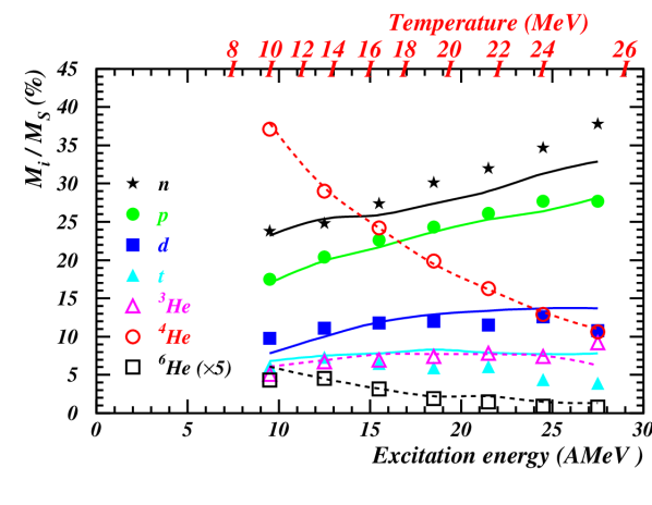
Figure 29: Composition of vaporized quasi-projectiles (in percent), formed in 95 MeV per nucleon ³⁶Ar+⁵⁸Ni collisions, as a function of their excitation energy per nucleon. Symbols are for data while the lines (dashed for He isotopes) are the results of the model. The temperature values used in the model are also given. From [20].

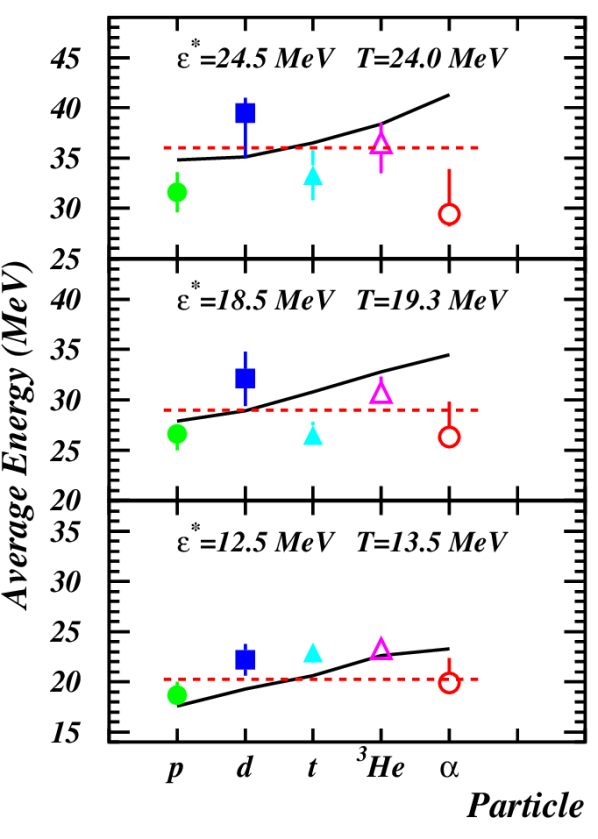
Figure 30: Average kinetic energies of particles emitted by vaporized quasi-projectiles at different excitation energies and formed in 95 MeV per nucleon ³⁶Ar+⁵⁸Ni collisions. Symbols are for data while full lines are the results of the model. The dashed lines refer to average kinetic energies of particles (3T/2) expected for an ideal gas at temperatures derived from the model. From [20].

Following this, to characterize the gas phase, nuclei which deexcite by emitting exclusively light particles (Z $\leq$ 2) were selected [201, 202, 203]. By doing this, one excludes the possible contamination from events of the phase coexistence region. The gas phase was characterized by comparison with a model, by studying the deexcitation properties of vaporized quasi-projectiles produced in ³⁶Ar+⁵⁸Ni reactions at 95 MeV per nucleon incident energy [20]. Chemical composition and average kinetic energies of the different particles are well reproduced by a quantum statistical model (grandcanonical approach) describing a real gas of fermions and bosons in thermal and chemical equilibrium. The evolution with excitation energy per nucleon of the composition of vaporized quasi-projectiles is shown in Fig. 30. Nucleon production increases with excitation energy whereas emission of alpha particles, dominant at lower excitation energies, strongly decreases. The regular behaviour observed is a strong indication that an abrupt change of phase does not occur in the considered excitation energy range. Note that an excluded volume correction due to finite particle size [79] (van der Waals-like behaviour) was found decisive to obtain the observed agreement. The consequence of the excluded volume correction is to favour neutrons, protons and alpha particles over the loosely bound particles like deuterons, tritons, ³He and ⁶He. In the model, the experimental range in excitation energy per nucleon of the source (9.5 to 27.5 MeV) was covered by varying the temperature from 10 to 25 MeV and the only free parameter, the excluded volume, was fixed at 3 $V_{0}$ in order to reproduce the experimental ratio between the proton and alpha yields at 18.5 MeV per nucleon excitation energy. $V_{0}$ is the volume of nuclei at normal density. The average kinetic energies of the different charged particles are also rather well reproduced over the whole excitation energy range (Fig. 30) but the model fails to accurately follow the dependence on the different species especially for alphas. The dashed lines in Fig. 30 indicate the average kinetic energies, 3T/2, expected for a free gas, which appear as a rather good approximation. This is due to the low density, around 0.15 - 0.2$\rho_{0}$, of vaporized nuclei at freeze-out. We are in the presence of a quantum weakly-interacting gas.

6 First-order phase transition in hot nuclei: from predictions to observations

This section is divided into five subsections. The first one presents the phase transition signatures related to the specific consequence of the non-additivity inherent to finite hot nuclei, i.e. an abnormal curvature of entropy. Then, consequences of finite size on scalings and critical behaviours will be discussed from fragment size distributions and fluctuations. In the third subsection results using Landau free-energy approach will be presented. In subsection four the most delicate point i.e. the nature of the dynamics of the phase transition will be discussed. Finally in subsection five the coherence of observed signatures will be summarized.

6.1 Phase transition signatures related to entropy convexity

In the physical situation encountered in the present studies concerning a first-order phase transition in isolated finite nuclear systems, extensive variables like energy and entropy are no longer additive due to the important role played by the surfaces of particles and fragments which are produced. As a consequence the number of states in the mixed/disordered region grows much faster with energy than the one associated to an ordered phase and this creates a convex intruder in the microcanonical entropy. In this context, coexistence does not refer to coexistence of two distinct phases in static physical contact within a single system but rather to coexistence of two phaselike forms among an ensemble of systems (see subsection 3.1).

The consequences of the curvature anomaly in the appropriate thermodynamic potential are now discussed. The entire coexistence region may be explored by varying the associated extensive variables. The most direct phase transition signature corresponds to a situation where the finite system is treated in the canonical ensemble, the value of $X$ may fluctuate as the system explores the phase space; the associated distribution at equilibrium is $P(X)$ $\sim$ exp($S(X)$ - $\lambda X$) where $\lambda$ is the Lagrange multiplier controlling the average. The distribution of $X$ acquires a bimodal character (see Fig. 31). That bimodality signature is the clearest indication that in finite systems the LG-type phase transition reveals itself as a coexistence between two types of events which manifest one of two phaselike forms.

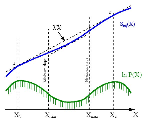
Figure 31: Canonical ensemble of finite systems. The bimodal equilibrium distribution of an extensive variable is given by $P(X)$ $\sim$ exp($S(X)$ - $\lambda X$). The figure shows the case when the Lagrange multiplier $\lambda$ is equal to the slope of the common tangent. From [5]).

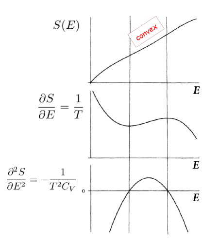
Figure 32: Microcanonical ensemble: evolution of entropy with energy (top), its first derivative 1/T (middle) and second derivative - 1/$T^{2}$$C_{V}$ (bottom), where T is the microcanonical temperature. Adapted from [50].

Another consequence of the entropy curvature anomaly appears by considering now the microcanonical ensemble with energy as extensive variable and is illustrated in Fig. 32: the convex intruder implies a backbending in the temperature (first derivative) and a negative branch for the heat capacity (second derivative) between two divergences. A quantitative illustration using the 2-dimensional Potts model can be found in [9]. As we will see, the backbending of caloric curves is not so direct to observe since caloric curves are affected by the specific dependence of the volume on the excitation energy. Indeed in the microcanonical situation for the LG phase transition, one is forced to introduce the volume which has to increase with energy to allow the system to explore the partitions belonging to the disordered phase. Conversely, negative heat capacity which always manifests by the presence of abnormally large kinetic energy fluctuations in the transition region should be easier to observe.

6.1.1 Entropy convexity and bimodality

For the macroscopic LG phase transition, the order parameter is the difference in density between the liquid and the gas. Since the density is related to both particle number and volume, for finite systems one may consider an ensemble in which these two extensive quantities are state variables. To further illustrate this point, one can consider an ensemble of $N$-particle systems for which the volume is not fixed but may fluctuate. In such an isobar canonical ensemble with the Lagrange multiplier $\lambda=P/T$ associated to volume, from the lattice-gas model (see 4.2.1) it is possible to define the statistical ensemble which contains the maximum of information on the system properties. It was done for $N$ = 216 [204, 72]. Fig. 33 displays volume and energy distribution and three associated projections. The bimodal structure clearly emerges. In the case of nuclear multifragmentation, related to the volume, a natural order parameter can be the size of the heaviest fragment emitted from highly excited nuclei [205, 206] (see also 6.2). Note that this observable provides an order parameter for a large class of transitions or critical phenomena involving complex clusters, from percolation to gelation, from reversible to irreversible aggregation. A priori that specific signature appears as robust and could be directly observed if a large excitation energy range can be covered in a single experiment.

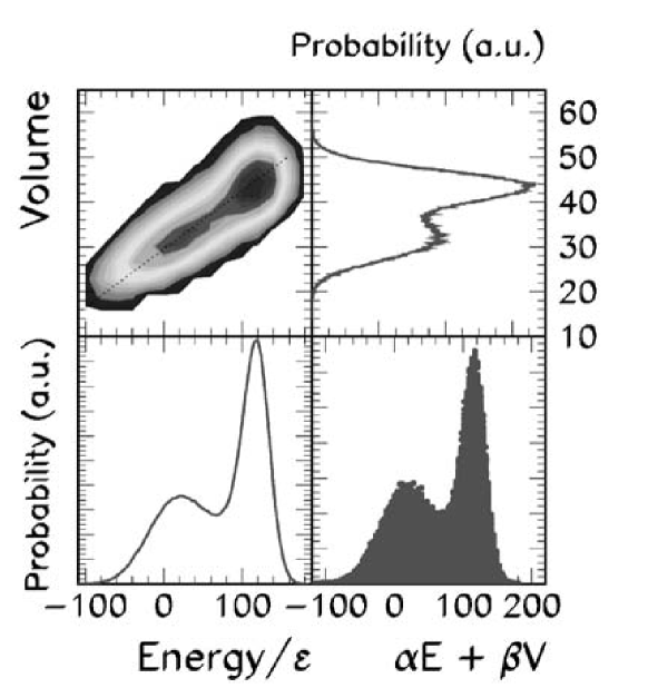
Figure 33: Lattice-Gas model in the isobar canonical ensemble. Event distribution in the volume V versus energy E plane in the first-order phase transition region with three associated projections: on the energy (bottom left), on the volume (top right) and on the line which connects the two maxima and can be seen as the best order parameter (bottom right). From [204].

A difficulty comes however from the sorting in the experimental data. The distribution of the energy deposit in collisions is obviously not that of the canonical ensemble and the distribution of the charge, $Z_{1}$, of the heaviest fragment has no meaning in terms of statistical mechanics. To cope with this problem, a simple procedure has been proposed in ref. [207]. The bimodality in the canonical two-dimensional probability distribution $p_{\beta}(E^{*},Z_{1})$ of a system of given size $Z_{s}$ at a first-order phase transition point reflects the convexity anomaly of the underlying density of states $W_{Z_{s}}(E^{*},Z_{1})$ [208, 209, 210] according to:

$$p_{\beta}(E^{*},Z_{1})=W_{Z_{s}}(E^{*},Z_{1})\exp(-\beta E^{*})Z_{\beta}^{-1},$$ (15)

where $\beta$ = $1/T$ and $Z_{\beta}$ is the partition function. In an experimental sample, the energy distribution is not controlled through a Boltzmann factor, but it is given by a collision and detector dependent functional $g(E^{*})$ according to:

$$p_{exp}(E^{*})\propto\int dZ_{1}W_{Z_{s}}(E^{*},Z_{1})g(E^{*}).$$ (16)

The convexity of the density of states can be directly inferred from the experimental distribution, by a simple weighting of the probabilities associated to each deposited energy:

$$p_{\omega}(E^{*},Z_{1})=\frac{p_{exp}(E^{*},Z_{1})}{p_{exp}(E^{*})}=\frac{p_{\beta}(E^{*},Z_{1})}{p_{\beta}(E^{*})}=\frac{W_{Z_{s}}(E^{*},Z_{1})}{W_{Z_{s}}(E^{*})}.$$ (17)

This procedure allows to get rid of the largely geometrical bias of entrance channel impact parameter distribution that naturally favours the lower part of the $E^{*}$ distribution. To produce a flat $E^{*}$ distribution according to Eq. (17), the $Z_{1}$ yield in each $E^{*}$ bin is weighted with a factor proportional to the inverse of the bin statistics.

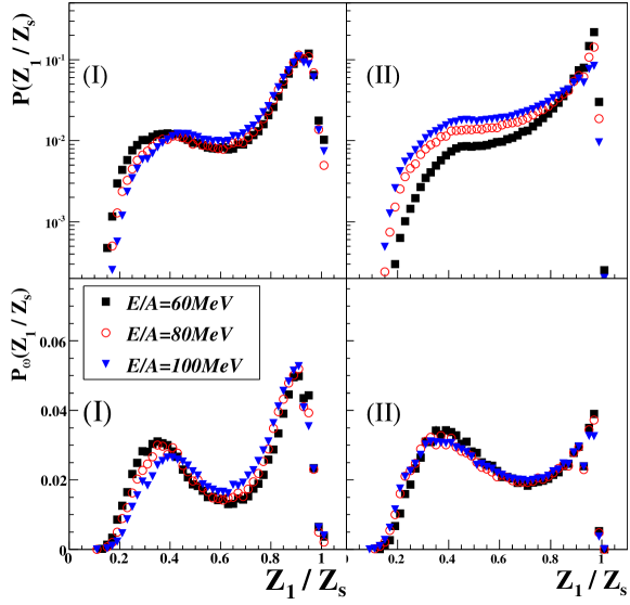
Figure 34: Upper part: measured distribution of the charge of the heaviest fragment normalized to the charge of the quasi-projectile size detected in ¹⁹⁷Au+¹⁹⁷Au collisions at three different bombarding energies. Lower part: weighted distributions obtained considering the same statistics for each excitation energy bin. (I) and (II) refer to two different quasi-projectile selections. From [210].

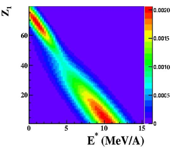
Figure 35: Event distribution in the atomic number of the heaviest fragment, $Z_{1}$, versus excitation energy per nucleon plane. The picture is constructed using the fit parameters extracted from the equivalent canonical distribution for selection II. The distance between the two maxima, “liquid” and “gas” peaks, projected on the excitation energy axis corresponds to the latent heat of the transition. From [211].

The results obtained with two different selection methods of quasi-projectiles produced in 60-100 MeV per nucleon incident energies ¹⁹⁷Au+¹⁹⁷Au semi-peripheral collisions [210] are displayed in Fig 34 (bottom). To take into account the small variations of the source size, the charge of the heaviest fragment was normalized to the source size, $Z_{s}$. A bimodal behaviour of the largest fragment charge emerges with both selections whatever the bombarding energy and for selection (II), results from different incident energies better superimpose. Fig 34 (top) also displays the original measured distributions before reweighting. It is important to note that the two selection criteria, (I) and (II), produce similar but not identical distributions even after weighting, meaning that a residual bias on the density of states exists. This is not surprising because any sorting procedure selects events according to observables correlated to the charge partitions. One may ask whether this inevitable bias prevents a sorting-independent extraction of the entropic properties of the system. To answer this question, comparison of information on the coexistence zone in the $(Z_{1},E^{*})$ plane (see Fig. 35) extracted from the two selection methods was done in [210]. Eq. (17) was solved for the canonical distribution $p_{\beta_{t}}(E^{*},Z_{1})$ at the transition temperature $\beta_{t}$ at which the two peaks of the energy distribution have the same height[72]. This is easily obtained in a double saddle point approximation [207]:

$$p_{\beta_{t}}(E^{*},Z_{1})=\sum_{i=l,g}N_{i}\frac{1}{\sqrt{det\Sigma_{i}}}\exp\left(-\frac{1}{2}\vec{x_{i}}\Sigma_{i}^{-1}\vec{x_{i}}\right).$$ (18)

where $\vec{x_{i}}=\left(E-E_{i},Z-Z_{i}\right)$, $\Sigma_{l}$ ($\Sigma_{g}$) represents the variance-covariance matrix evaluated at the “liquid” $l$ (“gas” $g$) solution, and $N_{l}$,$N_{g}$ are the proportions of the two phases. The weighted experimental distribution was fitted with the function $p_{w}(E^{*},Z_{1})=p_{\beta_{t}}(E^{*},Z_{1})/p_{\beta_{t}}(E^{*})$ which, using Eq. (18), is an analytic function. From the obtained parameter values and for selection (II), “liquid” and “gas” peaks have been respectively deduced; they are centred at 1.05 and 10.3 MeV per nucleon excitation energy and values of the largest fragment charge of 68.7 and 2.53. Those numbers seem very reasonable after the indications and comments that we were able to make on the appearance and composition of the gas phase (see subsection 5.2). The latent heat of the transition of the hot nuclei studied (Z$\sim$70) was also estimated from all available results [210]:

$\Delta E=E_{g}-E_{l}=8.1(\pm 0.4)_{stat}(+1.2-0.9)_{syst}$ MeV per nucleon.

Even though this study seems convincing, we must mention that other physical scenarios have been invoked to interpret the observation of bimodality: Jacobi transition of highly deformed systems [212] or self-organized criticality induced by nucleon-nucleon collisions [213, 214]. Recently BUU simulations suggest that, depending on the bombarding energy and impact parameter of the reaction, both entrance channel and exit channel effects can be at the origin of the bimodality [215]: fluctuations in the reaction mechanism induced by fluctuations in the collision rate for central collisions, which agrees with [214], as well as thermal bimodality directly linked to the LG phase transition for more peripheral collisions, which strongly supports the results just presented.

6.1.2 Entropy convexity and negative heat capacity

The observation of a plateau in nuclear caloric curves was experimentally proposed as a direct signature of a first-order phase transition (see Fig. 27) [165]. However, from a theoretical point of view, a plateau-like shape cannot be an unambiguous signature even if it is a strong indication of a physical change and if its observation can help to better define the energy domain of interest for the study of the phase coexistence. As mentioned before, measured caloric curves can be misleading because, depending on reactions involved and impact parameter domain, different curve shapes can be generated depending on the path followed in the microcanonical equation of state landscape. As examples, calculated caloric curves and normalized kinetic energy fluctuations (microcanonical isobar lattice gas model - 216 particles - see 4.2.1) [75] are displayed in Fig. 36. On the left hand side, landscapes of temperature and normalized kinetic energy fluctuations are shown in the plane energy per particle - Lagrange multiplier associated to volume $\lambda$ = $P/T$. If for temperature very different curve shapes are obtained depending on the path, normalized kinetic energy fluctuations related to microcanonical heat capacity are abnormally large in the coexistence region whatever the path. To better appreciate the situation, the right hand side of the figure shows the behaviours of caloric curves (upper panel) at constant pressure or at constant average volume in the subcritical region. At constant pressure a backbending is clearly seen whereas at constant average volume a smooth behaviour is observed with a slope change when entering the gas phase. In experiments one does not explore a caloric curve at constant pressure nor at constant volume, the different measured systems follow a path in the excitation energy - freeze-out volume plane and event by event freeze-out properties must be deduced from performing simulations to possibly derive relevant information. Constrained caloric curves will be discussed in 6.1.3.

Conversely the anomalously large fluctuation signal of kinetic energy (lower panel) is always seen, independently of the path, for systems undergoing a first-order phase transition. From this theoretical observation

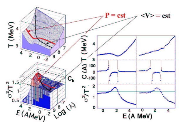
Figure 36: Isobar lattice gas model. Left part (top/bottom): temperature/ normalized kinetic energy fluctuations as a function of the energy per particle versus the Lagrange multiplier, $\lambda$ = $P/T$, associated to volume; the level corresponding to the canonical expectation $C_{k}=\sigma_{k}^{2}/T^{2}$ = 1.5 is shown. Right part: thermodynamic quantities in the microcanonical ensemble for a transformation at constant pressure and at constant average volume; caloric curves are displayed in upper panels, normalized kinetic energy fluctuations are compared to the canonical expectation (lines) in lower panels and middle panels display microcanonical heat capacities (symbols) compared to the estimation (lines) from Eq. (22). From [216]).

a method was proposed for measuring microcanonical heat capacity using partial energy fluctuations [67, 217, 75]. The prescription is based on the fact that for a given total energy, the average partial energy stored in a part of the system is a good microcanonical thermometer, while the associated fluctuations can be used to construct the heat capacity. From experiments the most simple decomposition of the total energy is in a kinetic part, $E_{k}$, and a potential part, $E_{pot}$, (Coulomb energy + total mass excess). However these quantities have to be determined at freeze-out and consequently it is necessary to trace back this configuration on an event by event basis. As discussed in section 4 the fragment properties entirely rely on the representation of the system at the freeze-out stage as non interacting fragments. The true configuration needs the knowledge of the freeze-out volume and of all the particles evaporated from primary hot fragments including the (undetected) neutrons. Consequently some working hypotheses are used, possibly constrained by specific experimental results (see for example [188, 72]). Then, the experimental correlation between the kinetic energy per nucleon $E_{k}$/$A$ and the total thermal excitation energy per nucleon $E^{*}$/$A$ of the considered system can be obtained event by event as well as the variance of the kinetic energy $\sigma_{k}^{2}$. Note that $E_{k}$ is calculated by subtracting the potential part $E_{pot}$ from the total energy $E^{*}$ and consequently kinetic energy fluctuations at freeze-out reflect the configurational energy fluctuations. In the microcanonical ensemble with total energy $E^{*}$ the total degeneracy factor is simply given by the folding product of the individual degeneracy factors $W_{k}=exp(S_{k}(E_{k}))$ and $W_{pot}=exp(S_{pot}(E_{pot}))$. One can then define for the total system as well as for the two subsystems the microcanonical temperatures and the associated heat capacities $C_{k}$ and $C_{pot}$. If we consider now the kinetic energy distribution when the total energy is $E^{*}$ we get

$$\noindent P_{E^{*}}(E_{k})=exp(S_{k}(E_{k})+S_{pot}(E^{*}-E_{k})).$$ (19)

Then the most probable kinetic energy $\overline{E_{k}}$ is defined by the equality of the partial microcanonical temperatures $T_{k}(\overline{E_{k}})$ = $T_{pot}(E^{*}-\overline{E_{k}})$ and $\overline{E_{k}}$ can be used as the microcanonical thermometer. An estimator of the microcanonical temperature of the system can be obtained by inverting the kinetic equation of state:

$$<E_{k}>=\langle\sum_{i=1}^{M}a_{i}\rangle T^{2}+\langle\frac{3}{2}(M-1)\rangle T$$

The brackets $\langle\rangle$ indicate the average on events with the same $E^{*}$, $a_{i}$ is the level density parameter and M the multiplicity at freeze-out. It may be noted that in this expression the same temperature is associated with both internal excitation and thermal motion of fragments. An estimate of the total microcanonical heat capacity is extracted using three equations.

$$\noindent C_{k}=\frac{\delta<E_{k}/A>}{\delta T},$$ (20)

is obtained by taking the derivative of $<E_{k}/A>$ with respect to $T$ and is equal to 1.5 in the canonical ensemble. Using a Gaussian approximation for $P_{E^{*}}(E_{k})$ the kinetic energy variance can be calculated as

$$A\sigma_{k}^{2}\simeq T^{2}\frac{C_{k}C_{pot}}{C_{k}+C_{pot}};$$ (21)

Eq. (21) can be inverted to extract, from the observed fluctuations, an estimate of the microcanonical heat capacity:

$$\noindent(\frac{C}{A})_{micro}\simeq C_{k}+C_{pot}\simeq\frac{C_{k}^{2}}{C_{k}-\frac{A\sigma_{k}^{2}}{T^{2}}}.$$ (22)

From Eq. (22) we can see that the specific microcanonical heat capacity $(C/A)_{micro}$ becomes negative if the normalized kinetic energy fluctuations $A\sigma_{k}^{2}/T^{2}$ overcome $C_{k}$. Fig. 36 (middle panels of right hand side) illustrates the results of such a procedure in the framework of the microcanonical lattice gas model. It is interesting to note that the constraint of energy conservation leads in the phase transition region to larger fluctuations than in the canonical case where the total energy is free to fluctuate. This is because the kinetic energy part is forced to share the total available energy with the potential part: when the potential part presents a negative heat capacity the jump from “liquid” to “gas” induces strong fluctuations in the energy partitioning.

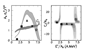
Figure 37: Left panel: normalized kinetic energy fluctuations and estimated $C_{k}$ values for quasi-projectile events produced in Au+Au collisions at 35 MeV per nucleon (grey zones) and for fused systems produced in central Au+C (black dots), Au+Cu (squares, triangles) and Au+Au reactions before (open stars) and after subtraction of 1 MeV per nucleon radial flow (black stars). Central panel: corresponding microcanonical heat capacities per nucleon. Grey zones indicate confidence regions. From [218]. Right panel: normalized kinetic energy fluctuations (filled circles) and estimated $C_{k}$ values (open circles) for quasi-projectile events produced in Au+Au collisions at 80 MeV per nucleon. From [219].

That procedure was applied by the MULTICS and INDRA collaborations on quasi-projectiles and on quasifusion nuclei produced respectively in semi-peripheral and central collisions in the incident energy range 30-80 MeV per nucleon [220, 221, 31, 218, 219]. Fig. 37 summarizes the results obtained by the MULTICS collaboration. On the left hand side it is seen that normalized kinetic energy fluctuations overcome $C_{k}$; the middle part of the figure illustrates the microcanonical negative heat capacities observed. On the right hand side of the figure, as an example, one result of the INDRA collaboration is also presented. We note that, with different selections of quasi-projectiles and different bombarding energies for the reaction Au + Au, measurements are compatible. These results provide a direct evidence of a first-order phase transition. In relation with the reconstruction at freeze-out, they have to be seen as semi-quantitative.

Exact microcanonical formulae, assuming that a classical treatment of the motion of products emitted at freeze-out is appropriate, are also proposed in [222] to calculate heat capacity or alternatively the second-order derivative of the system entropy versus energy. They only depend on the total kinetic energy and on the number of emitted products which have to be estimated event by event at freeze-out. However up to now this method was not used to derive information from data.

Before concluding this part one can indicate that questions are still under debate and concern the topology of the system at freeze-out. If the system is still relatively dense at freeze-out, which seems improbable if we refer to simulations from [157], which reproduce remarkably well experimental data and indicate freeze-out volumes in the range 3-6 times the volume at normal density, the fragment properties may be very different from the ones asymptotically measured and the question arises whether the energetic information measured on ground state properties can be taken for the freeze out stage [223]. Classical molecular dynamics calculations have shown that the ground state Q-value is a very bad approximation of the interaction energy of fragments in dense systems. This is due to the deformation of fragments and to the interaction energy when fragment surfaces touch each other. As a consequence, comparable kinetic energy fluctuations are obtained in the subcritical and supercritical regions of the Lennard-Jones phase diagram [224]. On the other hand calculations with a similar model, the Lattice Gas model, show that even in the supercritical region the correct fluctuation behaviour can be obtained if both the total energy and the interaction energy are consistently estimated with the same approximate algorithm as it is done in the experimental data analysis [225]. Concerning now the order of the transition, in certain theoretical calculations it appears that a negative heat capacity is not always incompatible with a continuous (second order) transition due to finite-size effects, either in a generic case [226] or for finite nuclei [227].

6.1.3 Constrained caloric curves

In Ref. [189, 157] freeze-out properties of multifragmenting quasifusion nuclei produced in central ¹²⁹Xe + ^natSn collisions at different beam energies (32, 39, 45 and 50 MeV per nucleon) have been estimated by means of a simulation based on all the available experimental information obtained with a very high degree of completeness for events, which is crucial for a good estimate of Coulomb energy. To check the overall physical coherence of this approach, a detailed comparison with a microcanonical statistical model (MMM - see section 4.2.2) was also made. Event by event, various quantities needed to build constrained caloric curves were deduced, namely the thermal excitation energy of quasifusion hot nuclei, $E^{*}$, the freeze-out volume $V$ and the total thermal kinetic energy at freeze-out $K$. With regard to the pressure at freeze-out, it can be derived within the microcanonical ensemble. Taking into account that $S=\ln Z=\ln\sum_{C}W_{C}$ and that $\partial W_{C}/\partial V=\left(M_{C}/V\right)W_{C}$, where $W_{C}$ is the statistical weight of a configuration , defined by the mass, charge and internal excitation energy of each of the constituting $M_{C}$ products at freeze-out, it comes out that

$$P/T=\left(\frac{\partial S}{\partial V}\right) = \frac{1}{\sum_{C}W_{C}}\sum_{C}\frac{\partial W_{C}}{\partial V}$$ (23)

$$= \frac{1}{V}\frac{\sum_{C}M_{C}W_{C}}{\sum_{C}W_{C}}=\frac{\langle M_{C}\rangle}{V}.$$

The microcanonical temperature is also easily deduced from its statistical definition [222]:

$$T=\left(\frac{\partial S}{\partial E}\right)^{-1} = \left(\frac{1}{\sum_{C}W_{C}}\sum_{C}W_{C}(3/2M_{C}-5/2)/K\right)^{-1}$$ (24)

$$= \langle(3/2M_{C}-5/2)/K\rangle^{-1}.$$

As $M_{C}$, the total multiplicity at freeze-out, is large,

$$\noindent T\thickapprox\frac{2}{3}\langle\frac{K}{M_{C}}\rangle$$ (25)

and the pressure $P$ can be approximated by

$$\noindent P=T\frac{\langle M_{C}\rangle}{V}\thickapprox\frac{2}{3}\frac{\langle K\rangle}{V}.$$ (26)

Knowing $\langle K\rangle$ and $V$ from simulations, pressure $P$ can be calculated for events sorted in each $E^{*}$ bin. The temperature $T_{kin}$ that we obtain from the simulations is identical to the microcanonical temperature of Eq. (25). One can also note that the free Fermi gas pressure exactly satisfies Eq. (26).

In simulations, Maxwell-Boltzmann statistics is used for particle velocity distributions at freeze-out and consequently the deduced temperatures, $T$ = $T_{kin}$, are classical. To build constrained caloric curves, authors of Ref. [228] have used a thermometer based on momentum fluctuations of emitted particles [185, 186] for which, for the first time, the quantum nature of particles is taken into account (see 4.4.2). Momentum fluctuations of protons were used and $\rho$ was estimated to $\rho\sim 0.4\rho_{0}$ from dynamical simulations, which corresponds to $\epsilon_{f}\sim$ 20 MeV. Systematic errors on $E^{*}$ and $T$ are discussed in [228].

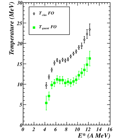
Figure 38: Caloric curves: classical temperature (open diamonds)/ quantum corrected temperature (full squares) from proton momentum fluctuations versus thermal excitation energy. Protons are thermally emitted at freeze-out. Error bars include statistical and systematic errors. From [228]).

Considering $E^{*}$ bins of 0.5 MeV per nucleon, to see the effect of the quantum nature of particles, Fig. 38 shows the caloric curve with temperatures from quantum fluctuations (full squares) compared to the one with classical temperatures derived from the simulation (open diamonds). They both exhibit a plateau with a significant difference for temperatures. For the quantum corrected caloric curve the plateau is observed around a temperature of 10-11 MeV on the $E^{*}$ range 5-10 AMeV. Then constrained caloric curves, which correspond to correlated values of $E^{*}$ and quantum corrected temperatures have been determined. $E^{*}$ values which are derived from experimental calorimetry have been corrected a posteriori using quantum temperatures instead of classical ones. Pressure values were also corrected using quantum temperatures in Eq. (26). In Fig. 39 (left hand side) constructed caloric curves for two average freeze-out volumes are displayed. As theoretically expected a monotonic behaviour of caloric curves is observed. Fig. 39 (right hand side) shows the caloric curves when pressure has been constrained within two domains: (1.3-4.5) and (4.5-7.9)x $10^{-2}$ MeV fm^-3. Again as theoretically expected, backbending is seen, especially for the lower pressure range. For higher pressures the backbending of the caloric curve is reduced and one can estimate its vanishing, indicating the critical temperature, around 13 MeV for the selected finite systems. So, constrained caloric curves confirm the previous signatures as far as a first-order phase transition for hot nuclei is concerned. Note that the caloric curve (quantum corrected temperature) of Fig. 38 resembles the caloric curves constrained in pressure of Fig. 39. This resemblance is not general and, in particular when rather light nuclei are involved, the shape of caloric curves is similar to the one of caloric curves constrained in average volume.

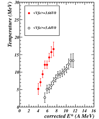
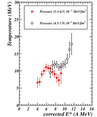
Figure 39: (Caloric curves (quantum corrected temperature versus corrected thermal excitation energy) constrained at average volumes (left) and for selected ranges of pressure (right). Error bars include statistical and systematic errors. From [228]).

Finally one can say a few words about the effect of $N/Z$ content on caloric curves. On the theoretical side the calculated temperature variation with isospin is small [229, 230, 231]. Experimentally, semi-peripheral collisions for 600 MeV per nucleon (¹²⁴Sn, ¹²⁴La, ¹⁰⁷Sn) + ^natSn [232] and 35 MeV per nucleon ⁷⁸Kr + ⁵⁸Ni and ⁸⁶Kr + ⁶⁴Ni [184] confirm a small isospin effect, with slightly higher temperatures for the neutron-richer systems. Conversely, in [233], and for light quasi-projectiles of known A and Z formed in 35 MeV per nucleon ⁷⁰Zn + ⁷⁰Zn, ⁶⁴Zn + ⁶⁴Zn and ⁶⁴Ni + ⁶⁴Ni reactions, measurable effects, with lower temperatures for neutron-richer nuclei were observed. Note that, unlike the ensemble of caloric curves presented in [234], none of those derived in [232, 184, 233] exhibits a plateau. In [233] the temperature linearly increases with energy between 2 and 8 MeV per nucleon, reaching 12 MeV at an excitation energy of 8 MeV per nucleon. Those measurements show again the necessity to constrain caloric curves to derive relevant information.

6.2 Criticality and correlation length

In general, thermodynamic features of systems near a critical point depend only on a small number of variables, mainly determined by the dimensionality and symmetry properties of the system, but are insensitive to details of the underlying microscopic properties [235]. They thus exhibit universality and the way in which certain physical properties (such as the difference between liquid and gas density for fluids, or the susceptibility for magnetic systems) approach their critical values are determined by critical exponents belonging to different universality classes. Scaling laws are frequently associated with critical systems, as the correlation length diverges and fluctuations occur at all length scales, manifesting a fractal, self-similar organization of matter.

In the early 1980s an experiment at the Fermi National Accelerator Laboratory led by a group from Purdue University was the first to provide high statistics, high resolution measurements of the inclusive mass distribution of fragments produced in high energy proton-nucleus collisions [236, 91]. The observation of a power-law,

$$\mathrm{yield}(A_{f})\propto A_{f}^{-\tau}$$ (27)

with exponent $\tau$ independent of the target mass strongly suggested the interpretation of fragment production as a critical phenomenon, by analogy with the well-known behaviour of real gases near the critical point, which exhibit cluster distributions with $\tau$ between 2.1 and 2.3, as described by the Fisher droplet model [90] (see 4.2.1). Since then many works have been devoted to the extraction of critical exponents from multifragmenting hot nuclei data, and results from different experiments are consistent with the LG phase transition universality class. Table 1 compiles some results for the following critical exponents: $\beta$, which controls how the difference between liquid and gas density goes to zero at the critical point; $\gamma$, which describes the divergence of the isothermal compressibility; $\tau$, the exponent of the mass-yield power law at the critical point; and $\sigma$, an exponent used by Fisher to relate cluster mass and surface energy (related to the dimensionality). The scaling of fragment yields based on the droplet model of [90] was even used to reconstruct the pseudo-coexistence curves at sub-critical densities for the phase transition [92, 237].

However, the question of criticality or the order of the phase transition is far from unambiguous when dealing with finite systems. In the fragmentation of small systems such as nuclei, critical behaviour has been shown to be compatible with a first-order phase transition, due to finite size effects [238]. There is no contradiction between the scenario of nuclear fragmentation inside the coexistence or the spinodal region associated with a first-order phase transition and the observation of pseudo-critical signals in fragment observables. The physical origin of the scaling behaviour at subcritical densities lies in the finite size of the system: for such small systems, correlations need only reach the same size as the system itself in order to mimic critical fluctuations with infinite correlation length.

Table 1: Theoretical values of critical exponents for the liquid-gas and percolation phase transition universality classes along with experimental values. For the experiments the critical excitation energy, $E_{C}*$, extracted from fitting fragment yields with the Fisher droplet model [90], is also given. QP and QF refer respectively to quasi-projectile and quasifusion hot nuclei.

	$E_{C}*$ [$A$MeV]	$\beta$	$\gamma$	$\tau$	$\sigma$
Liquid-gas	-	0.33	1.23	2.21	0.64
3D percolation	-	0.41	1.8	2.18	0.45
Au (1$A$GeV)+C [239, 240, 237]	4.6 $\pm$ 0.2	0.29 $\pm$ 0.02	1.4 $\pm$ 0.1	2.14 $\pm$ 0.06	0.68 $\pm$ 0.05
$\pi$(8 GeV/c) +Au [92]	3.8 $\pm$ 0.3	0.33 $\pm$ 0.25	-	2.18 $\pm$ 0.14	0.54 $\pm$ 0.01
Au (35 $A$MeV) + Au QP [241]	4.5 $\pm$ 0.2	0.38 $\pm$ 0.02	1.4 $\pm$ 0.3	2.2 $\pm$ 0.2
Xe (32$A$MeV)+Sn QF [219]	4.50 $\pm$ 0.03	-	-	2.09 $\pm$ 0.01	0.66 $\pm$ 0.01
Au (80$A$MeV)+Au QP[219]	4.20 $\pm$ 0.03	-	-	2.56 $\pm$ 0.02	0.66 $\pm$ 0.01

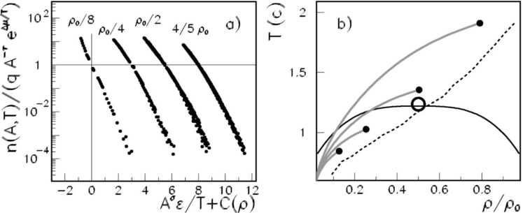
Figure 40: Application of the Fisher droplet model [90] to a canonical version of the Lattice Gas model (see [242] for details). (a) Cluster yields for different model densities scaled according to the Fisher ansatz; for each density the points are offset by a constant horizontal shift, $C(\rho)$, for clarity. (b) Thermodynamical coexistence line (full line) and line of maximum cluster size fluctuations leading to pseudocritical behaviour (dashed lines) from [238]. Grey lines: coexistence line reconstructed from fragment partitions. Adapted from [242].

Some consequences of this are illustrated in Fig. 40, taken from [242]. The canonical lattice gas model was used to calculate cluster mass yields $n(A,T)$ for a wide range of temperatures and densities both above and below the critical point. Then fits were performed to the cluster yields using Eq. (8) of section 4.2.1. It can be seen in Fig. 40(a) that the Fisher scaling ansatz works astonishingly well both below ($\rho<\rho_{0}/2$) and above ($\rho>\rho_{0}/2$) the critical density of the model, whereas the model is only strictly applicable to a subcritical system i.e. droplets surrounded by vapour. The extracted values for the critical exponents are, however, compatible (within finite size effects) with the universality class of the model. On the other hand, Fig. 40(b) shows the sub-critical coexistence curves (grey lines) deduced from the cluster yields using the same methods as applied to data in [92, 237]. For each density a different curve is obtained, terminating at (black points) different pseudo-critical temperatures which increase with the density of the system. Even for the calculations performed at the critical density of $\rho=\rho_{0}/2$ the deduced coexistence curve does not correspond to the thermodynamical one (black line) and overestimates the critical temperature. As shown in [242] the correct thermodynamics of the model are only retrieved for low densities and high temperatures for which the clusters behave as an ideal gas, as supposed by Fisher. When applied to data where no a priori knowledge of the density of the multifragmenting systems is available, the interpretation of results obtained with Fisher’s model is therefore not so straightforward.

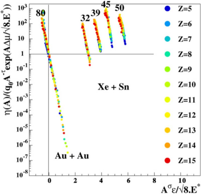
Figure 41: Fisher scaling of fragment yields applied to data for Au quasi-projectiles (in the reaction Au+Au at 80 MeV per nucleon incident energy) and for quasifusion nuclei produced in Xe+Sn reactions from 32 to 50 MeV per nucleon incident energies. Data for different Xe+Sn reactions have been shifted horizontally for clarity. From [219].

In [219] a large body of data was used to make a comprehensive survey of different signals of critical behaviour in multifragmentation, including Fisher scaling. As shown in Fig. 41, an excellent scaling is observed for fragment yields in the break-up of Au quasi-projectiles over a very wide range of excitation energies, which includes evaporative decay at the lowest excitation energies (fission events were excluded). A similar good scaling is also seen for multifragmenting hot nuclei formed in central Xe+Sn reactions, albeit over a much smaller range of excitation energies due to the reaction mechanisms involved. These data were shown elsewhere to be consistent with predictions based on the coexistence region of the nuclear phase diagram, not the critical point, i.e. spinodal decomposition [148, 243, 151, 244], negative heat capacity [188, 219], and, for the Au quasi-projectile data, bimodality of the order parameter [210]. Therefore for experimental data as for models, behaviour such as Fisher scaling of fragment yields, power laws, etc. is far from an unambiguous signal of criticality or of the order of the transition. Similar conclusions were reached in [245]. What is interesting to note here is that, although Fisher’s model applies only to subcritical clustering, the yield scaling is of equally good quality above the apparent critical temperature (i.e. above the horizontal line in Fig. 41). This is especially true for the data on quasifusion nuclei from Xe+Sn reactions for which almost all fragment yields are apparently compatible with supercritical temperatures. Indeed, only the data from the 32 MeV per nucleon incident energy reaction exhibit a subcritical branch while, for the higher bombarding energies, data move further and further away from the critical region. The astonishing fact is that although these results are not consistent in themselves with the Fisher model assumptions, they are consistent with other analyses of the same data using very different approaches and hypotheses. In [31] the negative branch of the heat capacity is clearly observed at 32 MeV per nucleon incident energy, less so at 39, and not significantly at all at 45 and 50 MeV per nucleon incident energies. Moreover the so-called “fossil signal” of spinodal decomposition which signs the systems’ exploration of the mechanically unstable region at the heart of the coexistence zone was shown to reach a maximum for 32 - 39 MeV per nucleon before decreasing to almost nothing at 50 MeV per nucleon incident energy[151, 244].

Another more general form of scaling law derived from the self-similar nature of critical systems concerns the universality of order parameter fluctuations, often referred to as $\Delta$-scaling [246, 247]. Given an observable $m$, the $\Delta$-scaling is observed when its probability distribution $P_{N}[m]$ for different system sizes $N$ can be reduced to a universal scaling function $\Phi(z_{(\Delta)})$ defined by

$$<m>^{\Delta}P_{N}[m] = \Phi(z_{(\Delta)})$$ (28)

$$z_{(\Delta)} = \frac{m-m*}{<m>^{\Delta}}$$ (29)

where $m*$ can be either the mode or the mean of the distribution. In the trivial case of Poissonian fluctuations (such as for a non-critical system or an observable $m$ not related to the order parameter), distributions scale with $\Delta=1/2$. At or above the critical temperature however, order parameter fluctuations scale like $\sigma_{m}\sim<m>$ and in this case the scaling law with $\Delta=1$ is expected (or $1/2<\Delta<1$ if $m$ is linearly related to the order parameter). A critical order parameter can therefore be identified by a change in the scaling properties of its fluctuations (change of $\Delta$). Moreover in the critical region the large-$z$ tail of the scaling function should decrease like $\Phi(z_{(1)})\sim\exp-z_{(1)}^{\nu}$ with exponent $\nu>2$, i.e. falling off faster than an exponential or gaussian tail.

As well as providing an alternative to critical exponent analysis in equilibrium systems, the authors of [246, 247] claimed that $\Delta$-scaling analysis has the advantage of being the only tool for the analysis of dynamical (non-equilibrium) systems as the scaling laws are independent of whether one is dealing with an equilibrium or a dynamical phase transition. They also stated that the $\Delta$-scaling cannot be defined for systems which exhibit a first-order phase transition, but it was later shown in [248] that the same pseudo-critical behaviour as seen for Fisher scaling also occurs for $\Delta$-scaling due to correlation lengths approaching the (finite) system size inside the coexistence region along the line of maximum fluctuations shown in Fig. 40. Other model calculations [249] indicate that such a scaling may appear for first-order transitions only if the system is sufficiently small, which is the case of all systems which are experimentally accessible in nuclear physics. A first application of the $\Delta$-scaling analysis to the multifragmenting quasifused systems formed in $Xe+Sn$ reactions was made in [250]. Both $\Delta=1/2$ and $\Delta=1$ scalings were observed in data. Fragment multiplicity distributions at all incident energies collapse onto to a single gaussian scaling function $\Phi(z_{(1/2)})$ with scaling $\Delta=1/2$ whereas the size (charge) of the largest fragment of each event, $Z_{max}$, exhibits the change of scaling expected for an observable closely related with an order parameter of a critical phase transition, between 32 MeV and 39 MeV per nucleon incident energies. On the other hand the large-$Z_{max}$ tail of the scaling functions did not show any sign of proximity to a critical region, falling off like $\exp(-z^{1.6})$.

The observed change of scaling law for $Z_{max}$ fluctuations, and thus its identification with a critical order parameter for multifragmentation, allows to establish in a model-independent way, i.e. without any a priori knowledge of the microscopic processes involved, that nuclear multifragmentation is more akin to the condensation of vapour than it is to the shattering of glass [251]. This is because all known critical phenomena with cluster degrees of freedom fall into two generic families, for each of which the order parameter is known:

• fragmentation scenarios in which clusters result by breaking the system into smaller pieces, rather like shattering glass or breaking a dinner plate. In this case the order parameter is the mean multiplicity of fragments; and

• aggregation scenarios in which clusters are built up from smaller pieces; the order parameter is the mean size of the largest cluster. This family includes the Fisher droplet model (and thus the LG phase transition), the Ising model and closely-related Lattice Gas model, and the percolation model.

System mass (size) dependence of $\Delta$-scaling for central symmetric collisions was studied in [252] where the behaviour of $Z_{max}$ as an order parameter was confirmed for the lighter systems Ar+KCl and Ni+Ni. It was shown that the bombarding energy at which the change of $\Delta$-scaling occurs decreases with the size of the system; for the heaviest system studied (Au+Au) only the $\Delta=1$ scaling is observed down to the lowest studied beam energy of 40 MeV per nucleon incident energy. For the first time the form of the scaling distribution in the $\Delta=1$ scaling regime was clearly identified as an extremal probability distribution, the Gumbel distribution

$$\Phi(z_{(1)})\sim\exp\left(-z-\exp\left(-z\right)\right).$$ (30)

Whereas the central limit theorem leads to the gaussian distribution for a sum of random variables, the Gumbel distribution belongs to a family of distributions representing the extrema of a set of random variables, and is characterized by an exponential tail on the extremal side (for large $z$ if $z$ is a maximum; for small $z$ if a minimum). In the $\Delta=1/2$ regime on the other hand the scaling function, although clearly much more symmetric than Eq. (30), could only be qualified as “quasi-gaussian”.

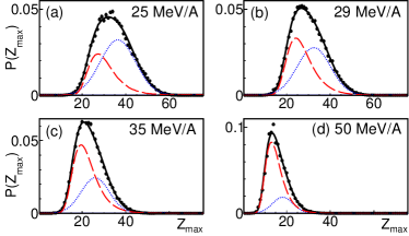
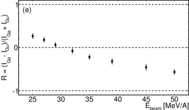
Figure 42: (a)-(d): Charge distributions of the largest fragment of each event $Z_{max}$ in central quasifusion collisions of Xe on Sn at the bombarding energies shown. Data: points; black line: fit of the distribution with an admixture of gaussian and gumbellian distributions; red dashed line: gumbellian component; blue dotted line: gaussian component. (e) Relative strengths of the two components, $R$ (see Eq. (31)), as a function of the beam energy. Adapted from [253].

The reason for the mass-dependence of the $\Delta$-scaling change and the exact form of the scaling function remained a mystery until it was realized that in the irreversible aggregation model represented by the Smoluchowski equations [254] the largest cluster size distribution $P(s_{max})$ can be reasonably approximated by a sum of gaussian and gumbellian distributions [255],

$$P(s_{max})=\frac{R+1}{2}f_{\mathrm{Gauss}}(s_{max})+\frac{1-R}{2}f_{\mathrm{Gumbel}}(s_{max}).$$ (31)

In this model, the cluster mass distributions evolve over time according to mass-dependent rates of aggregation or break-up, and after a time $t_{C}$, called the critical gelation time, a large (infinite in an infinite system) cluster appears corresponding to the sol-gel transition. The relative strength of the two components in the distribution of the largest cluster size, $R$, evolves with time in the model: at short timescales ($t\ll t_{C}$) when little aggregation has occurred $R\approx-1$, meaning that the Gumbel distribution dominates; at longer timescales ($t\gg t_{C}$) $R\rightarrow 1$ and the largest cluster size distribution becomes gaussian; at the critical gelation time $t_{C}$ (i.e. when fluctuations of the cluster size distribution are maximal) $R\approx-0.45$. This evolution of the distribution from gumbellian to gaussian means that the nature of the order parameter $s_{max}$ changes from extremal ($s_{max}$ corresponds to the largest of a set of uncorrelated, random clusters) to additive (the largest cluster results from the aggregation of smaller clusters). When applied to data on the largest fragment charge, the ansatz of Eq. (31) provides a far better fit to the $Z_{max}$ distributions for Xe+Sn central collisions than either of the two asymptotic distributions alone (Fig. 42(a)-(d)). Moreover the composition of the fit evolves in a regular way from gaussian to gumbellian ($R$ goes from positive to negative values in Fig. 42(e)) with increasing bombarding energy. Values of $R\approx-0.45$ corresponding to maximum fragment size fluctuations, analogous to the critical gelation time in the irreversible aggregation, occur at beam energies close to 39 MeV per nucleon incident energy, where the change of scaling law from $\Delta=1/2$ to $\Delta=1$ occurs.

By analogy with the irreversible aggregation model the authors of [253] therefore proposed that the exact form of the charge distribution of the largest fragment in nuclear multifragmentation, and hence its fluctuations, are also determined by the timescale of fragment formation in such reactions. The onset and increase of radial expansion at beam energies above 25 MeV per nucleon [87], essential to drive the system towards the onset of spinodal instability and initiation of the break-up into fragments [5], will also effectively shorten the time available for primary fragments to coalesce. Within this framework, the mass-dependence of the energy at which the $\Delta$-scaling law changes [252] can be ascribed to the entrance channel dependence of radial expansion in central collisions: for light systems such as Ar+KCl or Ni+Ni the bombarding energy required to achieve sufficient initial compression for there to be significant radial expansion is higher than for the heavier systems.

One can conclude this subsection by saying that now a coherent comprehensive view is obtained on the criticality signal subject for finite systems. This view is moreover reenforced by the consistence with other signatures, discussed up to now, of the coexistence region. As far as phase transition dynamics is concerned the aggregation scenario deduced recalls microscopic approaches in which fragments result from spinodal fluctuations occurring in the hot, expanding nuclear matter formed in collisions.

6.3 Landau free-energy approach

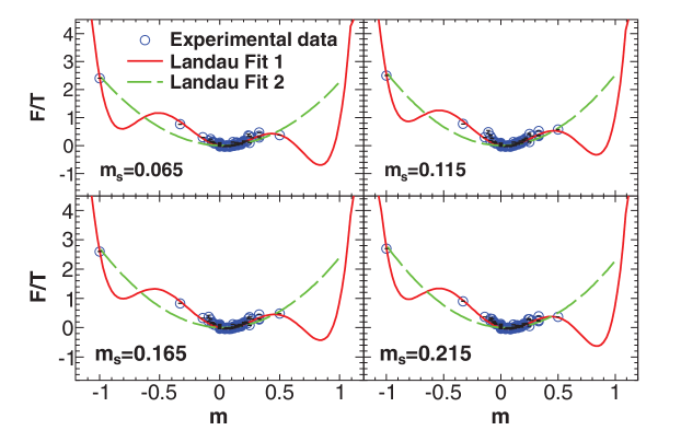
Figure 43: $F$/$T$ as a function of fragment neutron-proton asymmetry $m$ for an excitation energy of 6.5 MeV per nucleon of quasi-projectiles. Different panels correspond to different neutron-proton asymmetry ($m_{s}$) bins of quasi-projectiles. Full lines are fits to the data using the complete Landau free energy (first order phase transition) and dashed lines are fits which refer to single phase systems. Statistical errors are smaller than the points. From [256].

A new signature of first order phase transition was experimentally investigated using the Landau free-energy approach [256]. Quasi-projectiles formed in 35 MeV per nucleon ⁷⁰Zn + ⁷⁰Zn, ⁶⁴Zn + ⁶⁴Zn and ⁶⁴Ni + ⁶⁴Ni were reconstructed and data sorted in quasi-projectile asymmetry ($m_{s}=(N_{s}-Z_{s})/A_{s})$ and excitation energy bins in the range 3 - 9 MeV per nucleon. According to the modified Fisher model to take into account finite size effects, the free energy per nucleon of a fragment of mass $A$ normalized to the temperature of the quasi-projectile, $F/T$, can be derived from the fragment yield $Y~{}=~{}y_{0}A^{-\tau}e^{(-F/T)A}$; $y_{0}$ is a constant and $\tau$ is a critical exponent. In the Landau approach the free energy of a first order phase transition is extended in a power series in the order parameter $m$:

$$\noindent F/T=\frac{1}{2}am^{2}+\frac{1}{4}bm^{4}+\frac{1}{6}cm^{6}-\frac{H}{T}m,$$ (32)

with $m=(N_{f}-Z_{f})/A_{f}$; $N_{f}$, $Z_{f}$ and $A_{f}$ are the neutron, proton and mass numbers of the fragment respectively. The quantity $H$ is the conjugate variable of $m$ and $a$, $b$ and $c$ are fitting parameters which depend on the temperature, density or pressure of the fragmenting system. In the absence of $H$, the free energy $F/T$ is symmetric in the exchange of $m$ to $-m$ indicating that nuclear forces are invariant when exchanging $N_{f}$ in $Z_{f}$. In presence of $H$, which arises when the quasi-projectile is asymmetric in the composition ($m_{s}$), the symmetry is violated. More details can be found in [256]. In Fig. 43 $F/T$ values as a function of $m$ are displayed for quasi-projectiles at excitation energy of 6.5 MeV per nucleon and for different asymmetry ($m_{s}$) bins of quasi-projectiles (different panels). The value of $\tau$ = 2.3 $\pm$ 0.1 derived from previous works was used. Dashed lines are fits to data using only the first and last terms of Eq. (32), a case corresponding to single phase systems. Better fits (full lines) to data are obtained with the complete form of Eq. (32), which is the signature that quasi-projectiles are in the regime of a first-order phase transition. It is important to note that statistical error bars are smaller than the points.

6.4 Phase transition dynamics

The knowledge of the nature of the dynamics involved during phase transition in hot nuclei, i.e. fragment formation, is certainly the most delicate point. Two mechanisms have been proposed. On one side, stochastic mean field approaches predict the transition dynamics to follow the spinodal fragmentation scenario proposed very early on, triggered by phase-space fluctuations amplified in an unstable medium and, on the other side, molecular dynamics models (QMD, AMD) in which many-body correlations are sufficient to produce fragments at early times even in absence of unstable conditions. We have noticed in section 4 experimental evidence for a radial extra energy boost (radial expansion energy) associated to multifragmentation products. It can be attributed either to a dominant compression-expansion phase in central nucleus-nucleus collisions or to thermal pressure for more gentle collisions: hadron-nucleus or semi-peripheral nucleus-nucleus collisions. The system might then reach densities and temperatures that correspond to the unstable spinodal region where exponential amplification of density fluctuations leads to clusterization: an inhomogeneous mixture of fragments (normal density region), nucleons and light fragments (low density region). This can be seen as an analogue for phase separation in a finite system, for which spinodal decomposition would be the microscopic mechanism.

One must first visit the major theoretical progress which has been realized to understand and learn about spinodal fragmentation in the nuclear context especially for finite systems. A review can be found in Ref. [5].

What are the specificities of spinodal decomposition as far as nuclear matter is concerned?

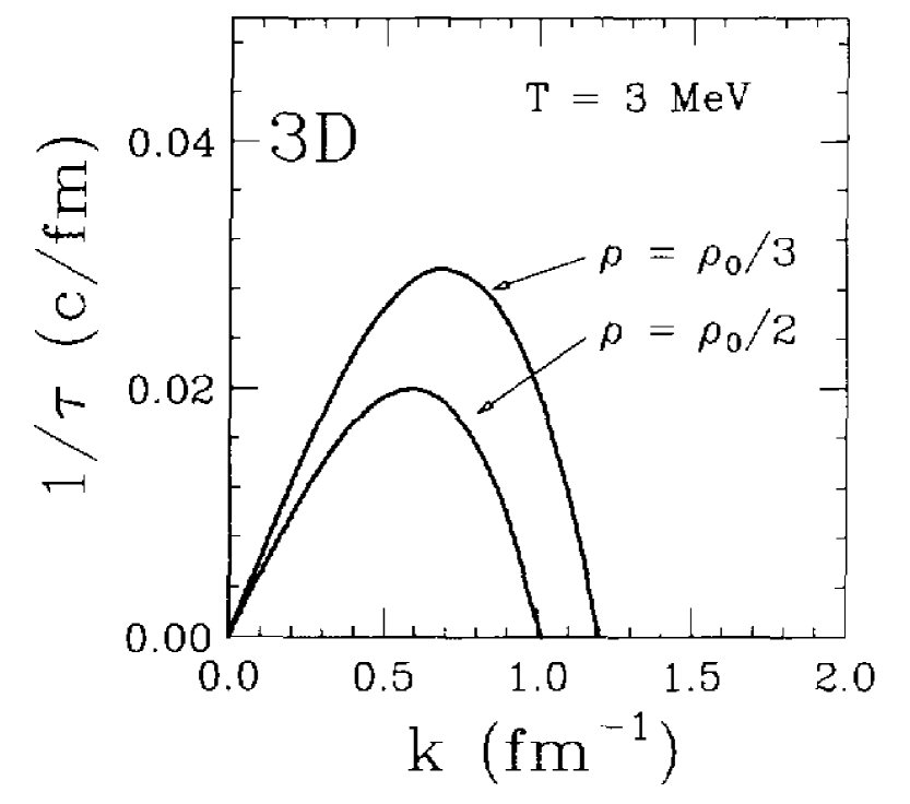
Figure 44: Nuclear matter dispersion relation at 3 MeV temperature for two different densities; $\rho_{0}$ is the normal density. From [28].

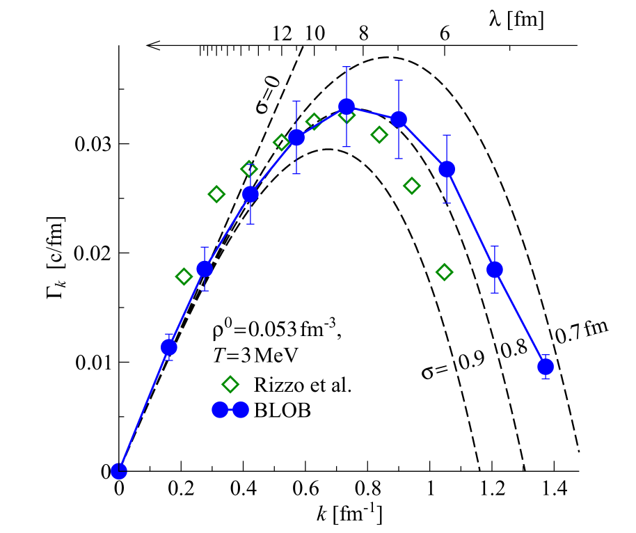
Figure 45: Nuclear matter dispersion relation at 3 MeV temperature for density around $\rho_{0}$/3 (full points). The dashed lines correspond to analytical predictions and diamonds to one dimension calculations from [257]. From [154].

Associated to negative compressibility the mechanically unstable spinodal region was investigated by studying the propagation of small density fluctuations [28, 258]. By analogy with optics, the nuclear dispersion relation can be calculated for different conditions of temperature and density by introducing the Boltzmann-Langevin equation with some stochasticity in the evolution of the one body density (BOB, BLOB - see 4.3.2). Within the linear response theory framework, if one expands the solution of the Boltzmann-Langevin equation as $f=f_{0}+\delta f$, where $f_{0}$ is a solution of the Boltzmann equation and $\delta f$ the fluctuating part, one finds the equation of motion $\partial\delta f/\partial t=-i\mathcal{M}\delta f+\delta I[f_{0}]$ at the leading order in $\delta f$. The extended RPA matrix operator $\mathcal{M}$ represents the combined linearized action of the effective field and of the average collision term. Inside the spinodal region the eigenvalues of the matrix $\mathcal{M}$ become imaginary. Consequently the fluctuations associated with a given eigenmode agitated by the source term $\delta I$ are exponentially amplified or suppressed, depending upon the sign of the imaginary part of the frequency. In the case of infinite nuclear matter the eigenmodes of the linearized dynamics are plane waves, characterized by a wavenumber $k$ and an imaginary eigenfrequency, which is the inverse of the instability growth time. Fig. 45 presents an example of nuclear dispersion relation at 3 MeV temperature for two different densities $\rho_{0}/2$ and $\rho_{0}/3$. Imaginary RPA frequencies are reported as a function of the wavenumber k of the considered perturbation. This dispersion relation exhibits a strong maximum at a given wavenumber followed by a cut-off at large k values. This cut-off reflects the fact that fluctuations with wavelength smaller than the range of the force cannot be amplified. The most unstable modes correspond to wavelengths lying around $\lambda\approx$  8-10 fm and the associated characteristic times are almost identical, around 30-50 fm/$c$, depending on density ($\rho_{0}/2$ - $\rho_{0}/8)$ and temperature (0 - 9 MeV) [28, 259]. Fig. 45 shows the results of the same study recently made in the framework of a numerical treatment of the Boltzmann-Langevin equation in which fluctuations are introduced in full phase space from inducing nucleon-nucleon collisions (BLOB simulation) [154]. Results obtained are very similar. A direct consequence of the dispersion relation is the production of “primitive” fragments with mass $A\approx\rho\lambda^{3}$. For the leading wavelengths, this corresponds to a distribution peaked around Ne nuclei. However this simple picture is expected to be largely blurred by several effects. The beating of different modes occurs. Coalescence effects due to the nuclear interaction between fragments before the complete disassembly are also expected [28].

For finite systems the situation is even more complicated. The presence of a surface introduces an explicit breaking of the translational symmetry. Fig. 46 shows the growth rates of the most unstable modes for a spherical nucleus of A = 200 with a Fermi shape profile and for two different central densities [260]. The growth rates are nearly the same for different multipolarities, $L$, up to a maximum multipolarity $L_{max}$ (see also [261]). This result indicates that the unstable finite system breaks into different channels depending on multipolarity [260]. Equal-sized “primitive” fragments are then expected to be produced with sizes in the range $A_{F}$/2 - $A_{F}$/$L_{max}$; $A_{F}$ being the part of the system leading to fragments during the spinodal fragmentation.

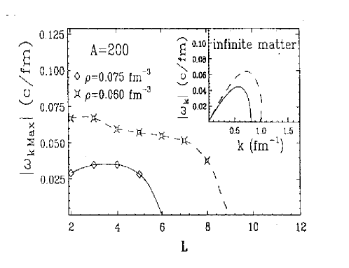
Figure 46: Growth rates of the most unstable modes for a spherical source with 200 nucleons as a function of the multipolarity $L$ and for two different central densities. From [260].

Moreover the finite system produced during the nucleus-nucleus collision has to stay or live long enough in the spinodal region ($\sim$ 3 characteristic times - 100-150 fm/c - for symmetric matter) to allow an important amplification of the initial density fluctuations. And in addition, experimentally, fragments are detected after secondary decay, which introduces a broadening of the fragment size distribution. Taking into account the accumulation of all these effects on the final extra production of equal-sized fragments, it is clear that any signature that spinodal fragmentation is responsible for the phase transition dynamics can only be what is called a fossil signature. A full simulation of the spinodal decomposition of quasifused sources using BOB simulations [151] already testified to this fact, with less than 1% of extra events with equal-sized fragments. It is the reason why the signature is difficult to observe experimentally. One can also note that the Coulomb potential has a very small effect on the growth rates of unstable collective modes except close to the border of the spinodal zone where it stabilizes very long wavelength unstable modes [262]. On the other hand, for a finite system, Coulomb interaction reduces the freeze-out time and enhances the chance to keep a memory of the dynamical instabilities; a similar comment can be made as far as collective radial expansion is concerned. Both effects push away the “primitive” fragments and reduce the time of their mutual interaction. So finally, even if expected extremely reduced, the presence of extra partitions with nearly equal-sized fragments is a candidate to sign the role of spinodal instability in multifragmentation.

Following early studies related to nearly equal-sized fragment partitions [263], an intra-event correlation method called higher order charge correlations [264] was proposed to enlighten any extra production of events with specific fragment partitions. The high sensitivity of the method makes it particularly appropriate to look for small numbers of events, as those expected to have kept a memory of spinodal fragmentation properties. All fragments of one event with fragment multiplicity $M=\sum_{Z}n_{Z}$, where $n_{Z}$ is the number of fragments with charge $Z$ in the partition, are taken into account. By means of the normalized first order:

$$\noindent\langle Z\rangle=\frac{1}{M}\sum_{Z}n_{Z}Z$$ (33)

and second order:

$$\sigma_{Z}^{2}=\frac{1}{M}\sum_{Z}n_{Z}(Z-\langle Z\rangle)^{2}$$ (34)

moments of the fragment charge distribution in the event, one may define the correlation function (CF):

$$\left.1+R(\sigma_{Z},\langle Z\rangle)=\frac{Y(\sigma_{Z},\langle Z\rangle)}{Y^{\prime}(\sigma_{Z},\langle Z\rangle)}\right|_{M}$$ (35)

Here, the numerator $Y(\sigma_{Z},\langle Z\rangle)$ is the yield of events with given $\langle Z\rangle$ and $\sigma_{Z}$ values. Because the measurement of the charge belonging to a given event is not subject to statistical fluctuations, expression (34) can be used rather than the “nonbiased estimator” of the variance, $\frac{1}{M-1}\sum_{Z}n_{Z}(Z-\langle Z\rangle)^{2}$, as proposed in  [264]. The exact identification of fragment charge up to at least $Z~{}\approx$ 25 is mandatory to use such intra-event correlation method for the proposed study. The denominator $Y^{\prime}(\sigma_{Z},\langle Z\rangle)$ represents the uncorrelated yield of pseudo-events and can be built in different ways. It was built in [264], as for classical correlation methods, by taking fragments at random in different events of the selected sample of a certain fragment multiplicity. This Monte-Carlo generation of the denominator $Y^{\prime}(\sigma_{Z},\langle Z\rangle)$ can be replaced by a fast algebraic calculation which is equivalent to the sampling of an infinite number of pseudo-events [265]. Its contribution to the statistical error of the correlation function is thus eliminated. However, owing to the way the denominator was constructed, only the fragment charge distribution $\mathrm{d}M/\mathrm{d}Z$ of the parent sample is reproduced but the constraints imposed by charge conservation are not taken into account. This has, in particular, a strong effect on the total charge bound in fragments, which makes the denominator yield distributions as a function of $\langle Z\rangle$ wider and flatter than those of the numerator [266]. Consequently, even in the absence of a physical correlation signal, the ratio (35) is not a constant equal to one. The correlations induced by the finite size of the system (charge conservation) distort the amplitude, or may even cancel other less trivial correlations. Therefore, a method for the evaluation of the denominator [265], based on the “intrinsic probability” of emission of a given charge, was proposed. It minimizes the effects just indicated and replicates all features of the partitions of the numerator, except the correlations due to other reasons than charge conservation. The principle of the method is to take into account in a combinatorial way the trivial correlations due to charge conservation. The probability to observe a given partition (${\bf n}:(n_{1},\ldots,n_{Z_{\rm max}})$), at a given total multiplicity, $m=\sum_{Z}n_{Z}$, is obtained by the multinomial formula. If the total charge is fixed ($Z_{\rm tot}=\sum_{Z}Z\,n_{Z}$), the partition probabilities are given by:

$$P({\bf n}|m)=\alpha\ m!\,\prod_{Z}\frac{{}^{\rm intr}P_{Z}^{n_{Z}}}{n_{Z}!}\ \delta_{Z_{\rm tot},\sum_{Z}Z\,n_{Z}}\ ,$$ (36)

where $\alpha$ is the normalization constant (so that $\sum_{n}P({\bf n}|m$) = 1) and $\delta$ is the Kronecker symbol. All the details can be found in [265, 151]. The intrinsic probability values, ${}^{\rm intr}P_{Z}$, are obtained by means of a recursive procedure of minimization.

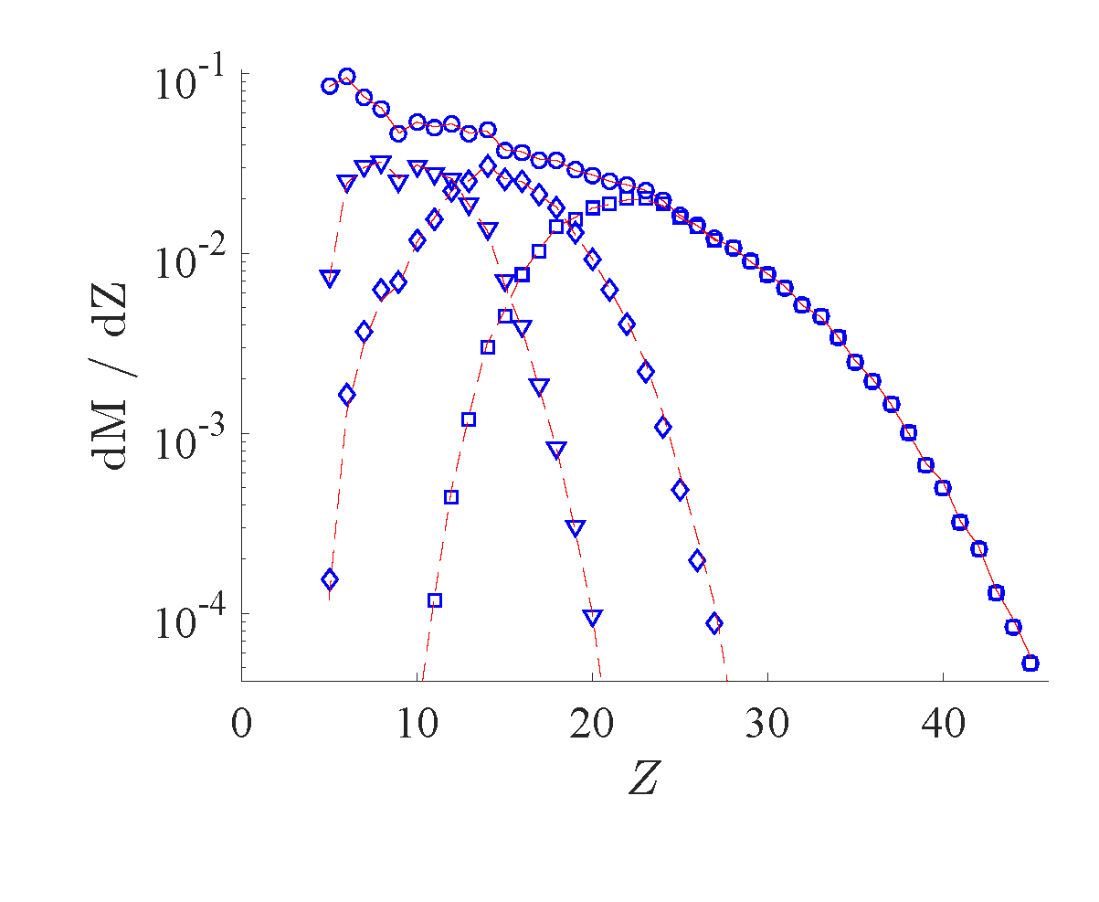
Figure 47: Experimental differential charge multiplicity distribution (circles) for quasifusion nuclei formed in central 32 MeV per nucleon ¹²⁴Xe + ¹¹²Sn reaction with fragment multiplicity, $M$, equal to 4. Experimental differential distributions for the first (squares), second (diamond) and third (triangles) heaviest fragments of partitions are presented too. The full and dashed lines, to be compared to data, correspond to the results of the intrinsic probability method for the fragment probabilities. From [244].

From experiments, about fifteen years ago, there were indications that multifragmentation may be induced by spinodal instabilities but the confidence level of the fossil signature was not sufficient (3 - 4 $\sigma$ at most), due to low statistics, to allow drawing any definitive conclusion [243, 151, 267]. Only very recently, studies obtained from very high statistics experiments ( a factor at least 10 to 15 higher as compared to previous ones) were performed aiming to give a final answer. At the same time, related isospin effects theoretically predicted were investigated. If spinodal instabilities are at the origin of multifragmentation, a reduction of instabilities for $N/Z$ asymmetric systems in relation with an increase of the instability growth time is theoretically predicted [40] (see Fig. 6). Intra-event charge correlations were performed on fragments emitted from multifragmenting quasifusion hot nuclei produced in central collisions between ^124,136Xe and ^112,124Sn at two bombarding energies, 32 and 45 MeV per nucleon [244]. The considered event samples for the study were those with fragment (Z $\geqq$ 5) multiplicities, $M$, from 3 to 6 which correspond to higher statistics. Fig. 47 shows one example on how the experimental fragment charge distributions are faithfully described by using the intrinsic probabilities, ${}^{\rm intr}P_{Z}$, which have been calculated independently for each incident energy, for each reaction and for the different fragment multiplicities. CF values greater than one were observed at very low $\sigma_{Z}$ ($<$ 1) but also for $\sigma_{Z}$ (1 - 2). This observation was used to fix the upper limit at 2 for the $\sigma_{Z}$ of events with nearly equal-sized fragments.

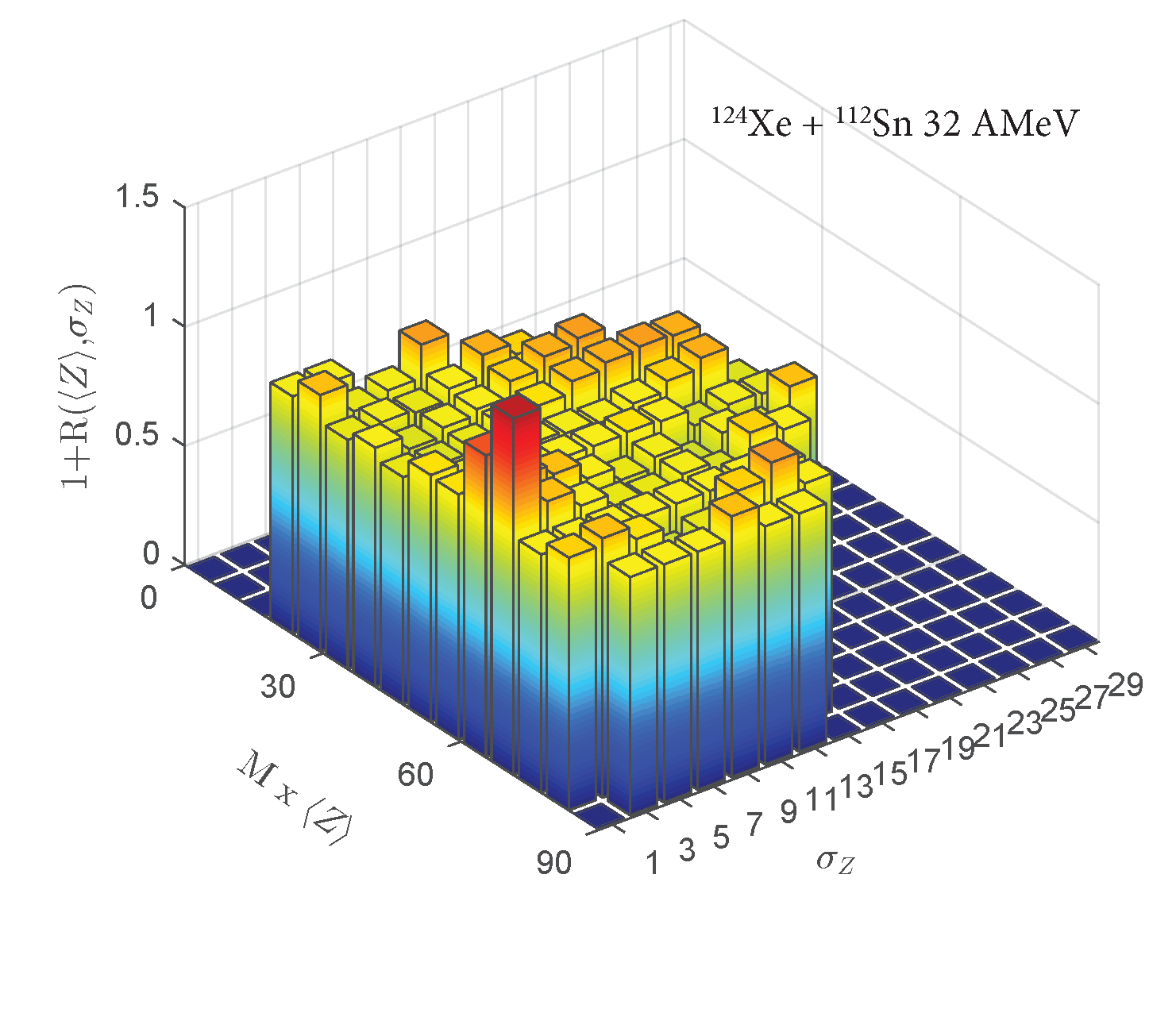
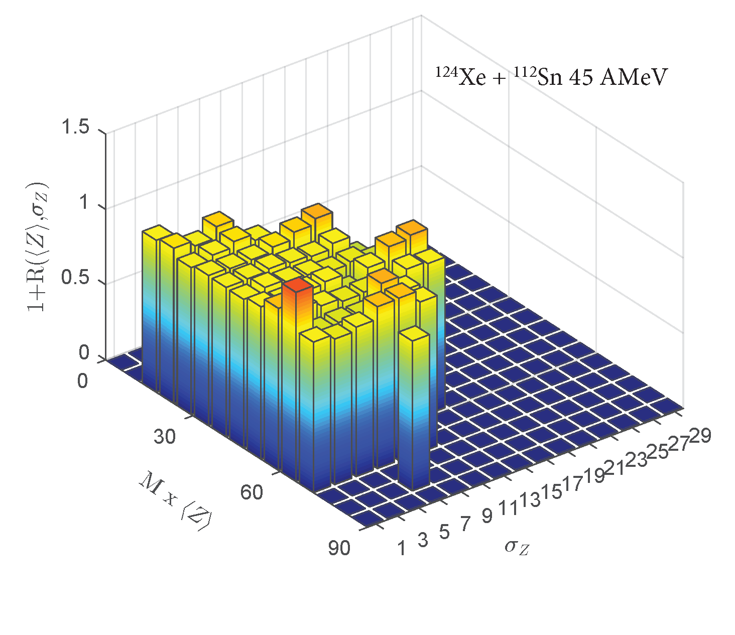
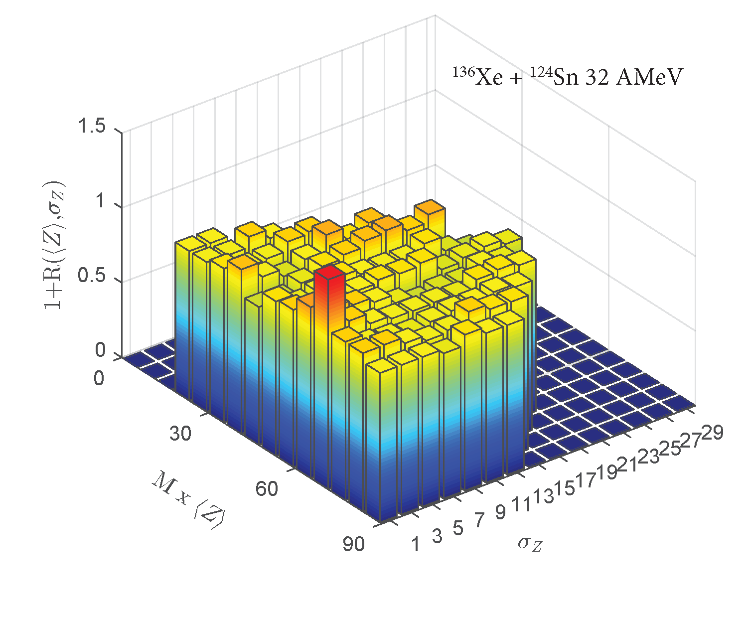
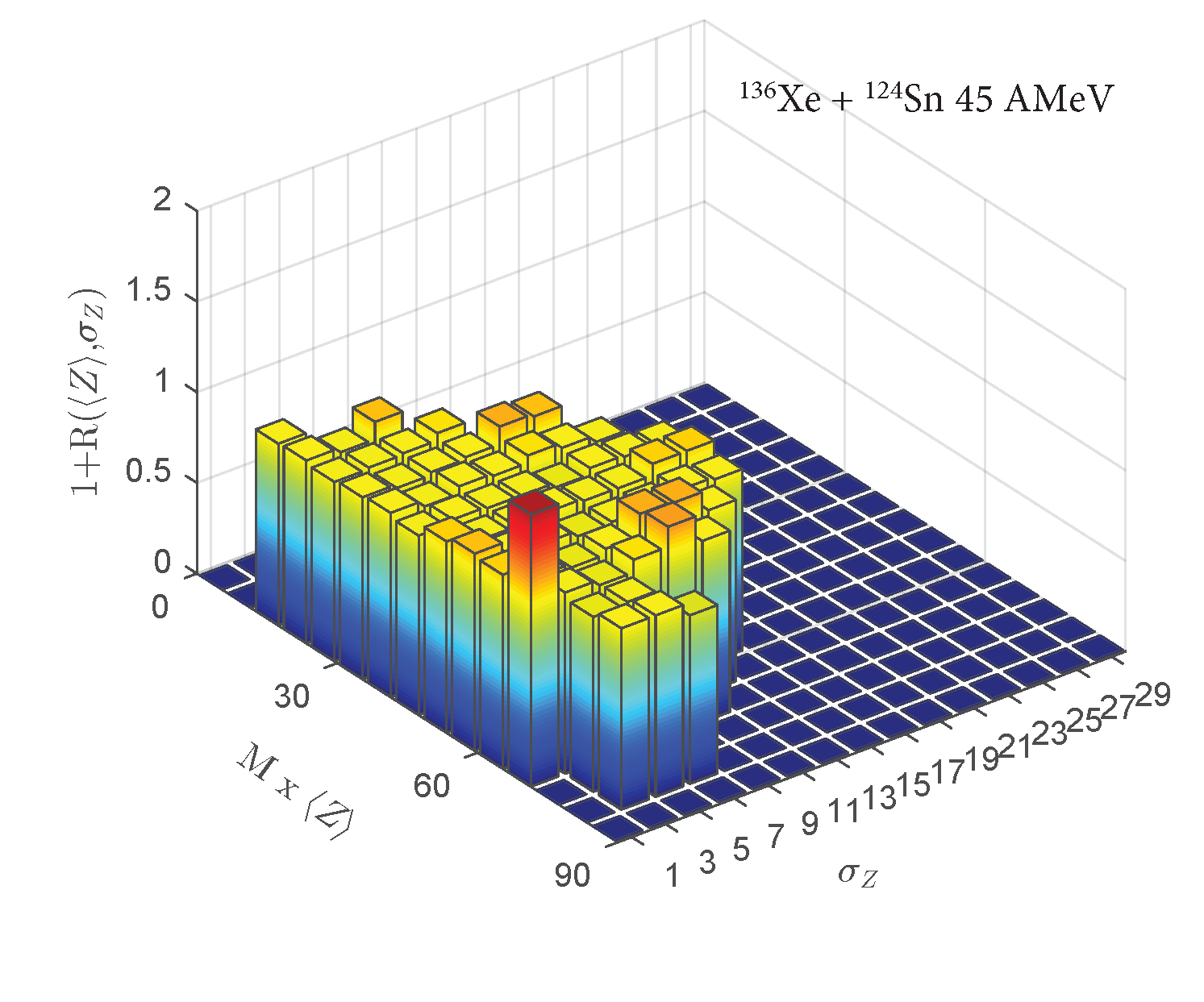
Figure 48: Experimental correlation functions for selected quasifusion events formed in central ^124,136Xe + ^112,124Sn collisions. Events with fragment multiplicities 3 to 6 are mixed. Correlation functions are calculated for a $\sigma_{Z}$ bin equal to 2 and a $M\times\langle Z\rangle$ bin equal to 6. The colour/grey scale for CFs has a maximum value for 1.6 which corresponds to dark red/dark grey. From [244].

The complementary contribution ($\sigma_{Z}$ 1 - 2) comes from the broadening of the fragment $Z$ distribution introduced by the deexcitation of primitive fragments (see [244] for details). For the first time, the limited ranges of $\langle Z\rangle$ contributing to CF peaks were also clearly observed, which verifies what is theoretically expected for finite systems i.e. $M\times\langle Z\rangle$ $\sim$ constant (see Table 1 of [244]). This observation also shows that some spurious peaks at low $\sigma_{Z}$ were present in previous experiments with low statistics. To better visualize global results, CFs were built for all events of a reaction at a given beam energy, whatever their multiplicity, by summing the correlated yields of all $M$ and by replacing the variable $\langle Z\rangle$ by $M\times\langle Z\rangle$. Uncorrelated yields are then constructed and weighted in proportion to real events of each multiplicity. Fig. 48 summarizes the results. For the four systems CF peaks are observed at low $\sigma_{Z}$. At 32 MeV per nucleon incident energy the neutron poor system exhibits two peaks with confidence levels greater around 6 - 7 $\sigma$ and the neutron rich one peak above 6 $\sigma$ and one around 3 $\sigma$, which definitively establishes the presence of spinodal fluctuations. At the higher incident energy the two systems have one peak with confidence level above 2 $\sigma$. Covered $M\times\langle Z\rangle$ domains are the same (60 - 72) for both reactions at 32 MeV per nucleon incident energy whereas at higher incident energy the neutron rich system covers a range a little bit higher (66 - 72) than the neutron poor one (54 - 66). Finally the percentages of events ($Y(\sigma_{Z},\langle Z\rangle)$/total number of events) and extra events (($Y(\sigma_{Z},\langle Z\rangle)$ - $Y^{\prime}(\sigma_{Z},\langle Z\rangle)$) /total number of events) are reported in Table 2.

Table 2: Numbers and percentages of events and extra events with $\sigma_{Z}<2$ for the different incident energies and reactions. Calculated errors are statistical. From [244].

E (AMeV)	reaction	events	(%)	extra events	(%)
32	$\@@nuc{124}{Xe}$+$\@@nuc{112}{Sn}$	1313	0.27	336	0.068 $\pm$ 0.004
32	$\@@nuc{136}{Xe}$+$\@@nuc{124}{Sn}$	1077	0.32	217	0.064 $\pm$ 0.004
45	$\@@nuc{124}{Xe}$+$\@@nuc{112}{Sn}$	1073	0.34	77	0.025 $\pm$ 0.003
45	$\@@nuc{136}{Xe}$+$\@@nuc{124}{Sn}$	68	0.030	15	0.0065 $\pm$ 0.0017

Within error bars, extra event percentages are similar for both systems at the lower incident energy. At higher incident energy we observe a strong reduction of percentages. The observed reduction for the more symmetric system is in good agreement with the negative heat capacity signatures observed experimentally (see 6.1.2) which fixed the upper limit of the coexistence zone (spinodal region) in the incident energy range 45-50 MeV per nucleon [31]. The large reduction of the signal observed for the neutron rich system, a factor ten between 32 and 45 MeV per nucleon, can be understood in terms of the expected $N/Z$ influence. Indeed, if spinodal instabilities are at the origin of the dynamics of multifragmentation, as said before, theoretical calculations predict a reduction of instabilities for asymmetric systems in relation with an increase of the instability growth time. More precisely, it is shown in [40] (see also Fig. 6) that, for $Sn$ isotopes, the most unstable modes associated to shorter instability growth times ($\simeq$ 50 fm/c) disappear when $N/Z$ changes from 1.40 to 1.64. If we consider that quasifusion systems produced by the collisions, with $N/Z$ varying from 1.27 to 1.50, have to stay long enough in the spinodal region ($\sim$ 3 characteristic times) to allow important amplification of the initial fluctuations, one can qualitatively understand the large extra reduction of the correlation signal for the neutron rich system at high incident energy as coming from insufficient reaction time. Such a situation also favours coalescence of primary fragments. Finally, note that the set of reaction trajectories in the density - temperature plane, close to the border of the spinodal region at 45 MeV per nucleon can be slightly different for the two reactions.

To summarize on these experimental results one can say that, using charge correlations, the fossil signature of spinodal instabilities i.e. the abnormal presence of nearly equal-sized fragments, even if very low as expected, was definitively established at a confidence level of around 6 - 7 $\sigma$. Associated to this weak signal, it is important to underline again the dominating role of chaotic/stochastic dynamics driven by spinodal instabilities for fragment formation, especially for finite systems. It has to do with beating of modes, breaking of translational symmetry and coalescence during the final step of fragment formation. In a more mathematical language, for fragment formation one can say that at an early stage the unstable modes are independent and their amplitudes evolve exponentially. Then, the modes become progressively coupled and the evolution grows more and more complicated as the non-linearities gain importance. Moreover, after the formation of nascent fragments which are in mutual nuclear interaction the system seeks to organize itself, it is the final coalescence phase. On the other hand it could be that spinodal fluctuations, even if present, do not play the dominating role which then would come from fluctuations due to many-body correlations (molecular dynamics models - see 4.3.1).

Considering the intrinsic weakness of the fossil signal, it would be valuable to have another signature. At the present time one can consider new studies with the advent of future accelerators which will provide beams covering a broad range in $N/Z$ ratios. Considering the LG phase transition for asymmetric nuclear matter analysed in a mean field approach, two different mechanisms of phase separation have been compared: equilibrium related to the highly chaotic character of collisions involved to produce hot nuclei and spinodal instabilities [268].

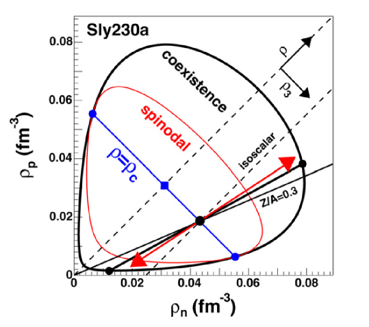
Figure 49: Coexistence and spinodal regions in the proton-neutron density plane at $T$ = 10 MeV. Illustration of phase separation inside the instability region for matter with a proton fraction $Z$/$A$ = 0.3 (see text). From [268].

The isospin properties of the phases are deduced from the free-energy curvature, which contains information on the average isospin of the phases and on the system fluctuations. The results are illustrated in Fig. 49 for neutron rich matter with $Z$/$A$ = 0.3 and a temperature $T$ of 10 MeV. If equilibrium is the origin of phase separation, the system will undergo separation according to Gibbs construction. The two phases, represented as black dots on the coexistence border do not belong to the line of constant proton fraction ($Z$/$A$ = 0.3). The liquid fraction is closer to symmetric matter than the gas phase. It is a consequence of the symmetry energy minimization in the dense phase. This unequal repartition of isospin between the two phases is the well-known phenomenon of isospin fractionation (see also 2.1.2). One can now study isospin fractionation if phase separation is driven by spinodal instabilities. This is the spinodal fragmentation and the local properties of the constrained entropy curvature determine the development into phase separation. The double arrow in Fig. 49 shows the results; the spinodal fragmentation leads to a more pronounced fractionation than equilibrium, the dense phase getting closer to the symmetric matter. This fact can be a possible new signature of the dynamics of the phase transition. However it appears as a very challenging task. For experimentalists large $Z$/$A$ values are required to have enough sensitivity. A robust reconstruction of primary fragments is also mandatory. Moreover future $A$ and $Z$ identification arrays, like for example FAZIA, are absolutely needed for such studies [269, 270]. On the theoretical side more realistic calculations involving collisions between nuclei are also essential.

6.5 Coherence of observed signals

To conclude this section one can say that it is now well-established that phase transitions can be identified in finite systems such as hot nuclei. However their manifestation is radically different to the behaviour expected in the thermodynamic limit. A first-order phase transition manifests itself in hot nuclei without real phase coexistence, these systems being too small to contain different homogeneous phases and the interface between them [49, 50]. Rather they exhibit characteristic behaviours determined by the same topological features of the microcanonical entropy (local convexities) which lead to phase separation in the thermodynamic limit.

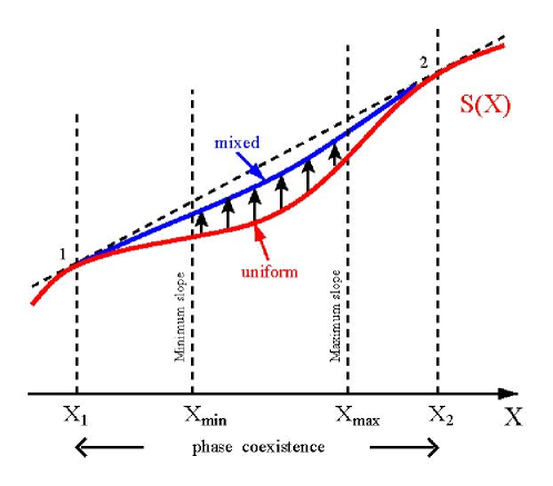
Figure 50: Isolated finite systems: the entropy function for a uniform unstable system (lower curve) has a local convexity region and the resulting equilibrium entropy function (upper curve) will always lie below the common tangent (dashed line). From [5].

For signal coherence, one can relate to Fig. 50. It shows the local convexity region (upper curve) as a function of one single extensive variable $X$ like energy; it also indicates the spinodal region (lower curve) located in between $X_{min}$ and $X_{max}$ and the mixed phaselike region in between $X_{1}$ and $X_{2}$. This means that if a signature of spinodal instabilities is observed one must observe correlatively the bimodality of an order parameter (canonical sampling), a negative microcanonical heat capacity and a pressure constrained caloric curve with backbending, all related to the resulting equilibrium entropy function with convexity (upper curve). On the other hand, if spinodal instabilities are not responsible for phaselike separation and if a phase transition occurs, the other signatures must be correlatively observed. Moreover, for hot nuclei, critical behaviours are expected to be observed in the coexistence region due to the finite size of the system which leads to the same effect as a diverging correlation length in an infinite system.

From the body of phase transition signals discussed in this section, a full coherence of phase transition signals is observed. Starting from a weak signature of the phase transition dynamics (spinodal instabilities), the three expected correlated signals: bimodality of an order parameter (canonical sampling), negative microcanonical heat capacity and pressure constrained caloric curve with backbending have been observed. Moreover, critical exponents are also observed in the coexistence region. From quasifusion hot nuclei produced in central Xe+Sn collisions, for which information is the most complete, the thermal excitation energy domain 3.5 - 9.5 MeV per nucleon corresponds to the spinodal - coexistence region.

From universal fluctuations ($\Delta$-scaling) the size of the largest fragment of each partition was determined as an order parameter in coherence with the bimodality observed. The determination of such an order parameter which corresponds to an aggregation scenario, in addition to the observed system mass and bombarding energy dependence of the associated probability distributions which was linked to the onset and importance of radial collective energy due to expansion, also agrees with the process of spinodal fragmentation.

7 Conclusions

When the first study programs concerning a phase transition for hot nuclei were proposed, many pessimistic comments were made related with the difficulties to overcome, for example:
(i) - produced by collisions, hot nuclei in themselves are transient in nature;
(ii) - the highly dynamical nature of collisions between objects with a small number of constituents and some direct processes involved between nucleons seem incompatible with the application of well known thermodynamic concepts used to describe phase transitions for macroscopic systems;
(iii) - phase transitions cannot be defined for finite systems, even talking about “phases” for small systems like nuclei makes no sense.

The difficulties have been largely overcome on both theoretical and experimental sides. The key words for that have been: thermodynamics of non-additive systems, stochastic mean field approach, chaoticity and large covering of phase space, statistical models, universal fluctuations, sophisticated 4$\pi$ detectors, data selection, homogeneous event samples, exclusive analysis, quasicomplete events, collective variables on an event-by-event basis, intra-event correlations. Close collaboration between theorists and experimentalists has also been very valuable in defining strategies for analysing data.

As we have seen all along this review an enormous progress has been done even if some points can be deeper investigated.

It is important to recall here one last time that signals of phase transition for finite systems are only meaningful at the level of statistical ensembles constructed from the outcome of many carefully selected collisions, and this fact must always be borne in mind for correct interpretation. The properties at the freeze-out instant of a very large number of similar collisions reveal the fingerprints of the phase transition.

Whatever the results of a limited number of experiments given the cumbersome nature of the experiments and the analyses, the expected coherence between signals indicating a first-order phase transition has been observed. There is also now a good understanding of the observation of critical exponents in the region of coexistence compatible with the class of universality. The theory of universal fluctuations ($\Delta$-scaling) was used to determine that an order parameter of the phase transition for hot nuclei is the size of the largest fragment of each partition which is coherent with the bimodality observed for this fragment size. For the phase transition dynamics the presence of spinodal fluctuations was definitively established in coherence with aggregation process deduced from fluctuations of the largest fragment size. However the weakness of the signature could also indicate that chaoticity is dominating to produce fragments.

To progress further, besides a few proposed new signatures to be confronted to data, the main effort has to be made from the experimental side by identifying not only charge but also mass of fragments. Knowing $Z$ and $A$ one would be able to reduce or suppress hypotheses made to evaluate freeze-out properties which are, as we have seen, key points to derive quantitative information. It would become possible to disentangle for fragments Coulomb repulsion from collective radial expansion and consequently to experimentally access this energy component obtained up to now from a parameter of statistical models fitting well the data. By largely varying the proportions of neutrons and protons involved in collisions new signatures related to the phase transition for nuclei are predicted: the distillation, which makes the ‘gas’ phase more asymmetric than the ‘liquid’ phase (even more asymmetric for spinodal decomposition as compared to phase equilibrium). By measuring the isotopic composition of all the fragments it would become possible to better identify the two phaselike forms and determine by a new way the dynamics of the transition. Finally, on the theoretical side a full quantal description of collisions would be the supreme outcome; for example at present radial collective energy due to thermal pressure cannot be calculated.

References

- [1] G. F. Bertsch et al., Phys. Lett. B 126 (1983) 9.
- [2] P. Chomaz et al. (eds.), Dynamics and Thermodynamics with Nuclear Degrees of Freedom, vol. 30 of Eur. Phys. J. A, Springer, 2006.
- [3] D. H. E. Gross, Microcanonical Thermodynamics - Phase Transitions in “Small” Systems, World Scientific, Singapore, 2001.
- [4] T. Dauxois et al. (eds.), Dynamics and Thermodynamics of Systems with Long Range Interactions, vol. 602 of Lecture Notes in Physics, Springer-Verlag, Heidelberg, 2002.
- [5] P. Chomaz et al., Phys. Rep. 389 (2004) 263.
- [6] R. T. de Souza et al., P. Chomaz et al. (eds.) Dynamics and Thermodynamics with Nuclear Degrees of Freedom, Springer, 2006, vol. 30 of Eur. Phys. J. A, 275–291.
- [7] L. G. Moretto et al., Ann. Rev. of Nuclear and Particle Science 43 (1993) 379.
- [8] J. Bondorf et al., Phys. Rep. 257 (1995) 133.
- [9] D. H. E. Gross, Phys. Rep. 279 (1997) 119.
- [10] L. G. Moretto et al., Phys. Rep 287 (1997) 249.
- [11] C. B. Das et al., Phys. Rep. 406 (2005) 1.
- [12] V. E. Viola et al., Phys. Rep. 434 (2006) 1.
- [13] B. Borderie et al., Prog. Part. Nucl. Phys. 61 (2008) 551.
- [14] G. Giuliani et al., Prog. Part. Nucl. Phys. 76 (2014) 116.
- [15] G. F. Bertsch, Z. Phys. A 289 (1978) 103.
- [16] C. Toepffer et al., Phys. Rev. C 25 (1982) 1018.
- [17] J. Cugnon, Phys. Lett. B 135 (1984) 374.
- [18] W. Cassing, Z. Phys. A 327 (1987) 447.
- [19] D. Jouan et al., Z. Phys. A 340 (1991) 63.
- [20] B. Borderie et al., Eur. Phys. J. A 6 (1999) 197.
- [21] J. Margueron et al., Phys. Rev. C 97 (2018) 025805.
- [22] K. A. Bugaev et al., Phys. Rev. C 62 (2000) 044320.
- [23] K. A. Bugaev et al., Phys. Lett. B 498 (2001) 144.
- [24] H. Jaqaman et al., Phys. Rev. C 27 (1983) 2782.
- [25] H. R. Jaqaman et al., Phys. Rev. C 29 (1984) 2067.
- [26] L. P. Csernai et al., Phys. Rep. 131 (1986) 223.
- [27] H. Müller et al., Phys. Rev. C 52 (1995) 2072.
- [28] M. Colonna et al., Nucl. Phys. A 613 (1997) 165.
- [29] H. Heiselberg et al., Phys. Rev. Lett. 61 (1988) 818.
- [30] J. López et al., Phys. Lett. B 219 (1989) 215.
- [31] B. Borderie, J. Phys. G: Nucl. Part. Phys. 28 (2002) R217.
- [32] V. Baran et al., Phys. Rep. 410 (2005) 335.
- [33] B.-A. Li et al., Phys. Rep. 464 (2008) 113.
- [34] C. J. Horowitz et al., J. Phys. G 41 (2014) 093001.
- [35] M. Baldo et al., Prog. Part. Nucl. Phys. 91 (2016) 203.
- [36] V. Baran et al., Nucl. Phys. A 632 (1998) 287.
- [37] J. Margueron et al., Phys. Rev. C 67 (2003) 041602.
- [38] B.-A. Li et al., Nucl. Phys. A 699 (2002) 493.
- [39] J. N. De et al., Phys. Rev. C 59 (1999) 1.
- [40] M. Colonna et al., Phys. Rev. Lett. 88 (2002) 122701.
- [41] M. Colonna et al., Phys. Rev. C 78 (2008) 064618.
- [42] J. Rizzo et al., Phys. Rev. C 76 (2007) 024611.
- [43] E. Bonnet et al., Phys. Rev C 89 (2014) 034608.
- [44] J. Xu et al., Phys. Rev. C 93 (2016) 044609.
- [45] A. J. Cole et al., J. Phys. G: Nucl. Part. Phys. 23 (1997) 457.
- [46] P. Chomaz et al., P. Chomaz et al. (eds.) Dynamics and Thermodynamics with Nuclear Degrees of Freedom, Springer, 2006, vol. 30 of Eur. Phys. J. A, 317–331.
- [47] D. Lynden-Bell et al., Mont. Not. of the Royal Astro. Soc. 138 (1968) 2495.
- [48] W. Thirring, Z. Phys. A 235 (1970) 339.
- [49] P. Labastie et al., Phys. Rev. Lett. 65 (1990) 1567.
- [50] D. J. Wales et al., Phys. Rev. Lett. 73 (1994) 2875.
- [51] R. E. Kunz et al., Phys. Rev. E 49 (1994) 1895.
- [52] H. P. Cheng et al., Phys. Rev. A 46 (1992) 791.
- [53] F. Gulminelli et al., Phys. Rev. E 66 (2002) 046108.
- [54] H. Touchette, Phys. Rep. 478 (2009) 1.
- [55] A. Campa et al., Phys. Rep. 480 (2009) 57.
- [56] D. P. Sheehan et al., Physica A 370 (2006) 461.
- [57] T. Mori, J. Stat. Mech. 10 (2013) P10003.
- [58] R. Ellis et al., J. Stat. Phys. 101 (2000) 999.
- [59] J. Barre et al., Phys. Rev. Lett. 87 (2001) 030601.
- [60] H. Touchette, Europhys. Lett. 96 (2011) 50010.
- [61] L. van Hove, Physica 15 (1949) 951.
- [62] M. S. S. Challa et al., Phys. Rev. A 38 (1988) 6324.
- [63] H. Touchette et al., Physica A 340 (2004) 138.
- [64] P. Chomaz et al., T. Dauxois et al. (eds.) Dynamics and Thermodynamics of Systems with Long Range Interactions, Springer-Verlag, Heidelberg, 2002, vol. 602 of Lecture Notes in Physics, 68–129.
- [65] D. H. E. Gross, Z. Phys. B 104 (1997) 541.
- [66] R. E. Kunz et al., Phys. Rev. Lett. 71 (1993) 3987.
- [67] P. Chomaz et al., Nucl. Phys. A 647 (1999) 153.
- [68] M. Bixon et al., J. Chem. Phys. 91 (1989) 1631.
- [69] D. H. E. Gross, Physica A 365 (2006) 138.
- [70] N. Bohr, Nature 137 (1936) 344.
- [71] V. Weisskopf, Phys. Rev. 52 (1937) 295.
- [72] F. Gulminelli, Ann. Phys. Fr. 29 (2004) No 6.
- [73] J. Randrup et al., Nucl. Phys. A 356 (1981) 223.
- [74] D. H. E. Gross, Rep. Prog. Phys. 53 (1990) 605.
- [75] P. Chomaz et al., Phys. Rev. Lett. 85 (2000) 3587.
- [76] D. Hahn et al., Phys. Rev. C 37 (1988) 1048.
- [77] D. Hahn et al., Nucl. Phys. A 476 (1988) 718.
- [78] J. Konopka et al., Phys. Rev. C 50 (1994) 2085.
- [79] F. Gulminelli et al., Nucl. Phys. A 615 (1997) 117.
- [80] A. H. Raduta et al., Phys. Rev. C 55 (1997) 1344.
- [81] S. E. Koonin et al., Nucl. Phys. A 474 (1987) 173.
- [82] C. B. Das et al., Phys. Rev. C 64 (2001) 017601.
- [83] P. Lautesse et al., Eur. Phys. J A 27 (2006) 349.
- [84] S. Nagamiya, Nucl. Phys. A 488 (1988) 3c.
- [85] A. Schuttauf et al., Nucl. Phys. A 607 (1996) 457.
- [86] J. Łukasik et al., Phys. Lett. B 566 (2003) 76.
- [87] E. Bonnet et al., Nucl. Phys. A 816 (2009) 1.
- [88] D. Stauffer et al., Introduction to Percolation Theory, Taylor & Francis Publishers, London, 1994.
- [89] F. Gulminelli et al., Int. J. Mod. Phys. E 8 (1999) 1.
- [90] M. E. Fisher, Physics 3 (1967) 255.
- [91] A. S. Hirsch et al., Phys. Rev. C 29 (1984) 508.
- [92] J. B. Elliott et al., Phys. Rev. Lett. 88 (2002) 042701.
- [93] X. Liu et al., Phys. Rev. C 97 (2018) 014613.
- [94] J. P. Bondorf et al., Phys. Rep. 15 (1974) 83.
- [95] D. H. E. Gross et al., Phys. Rep. 45 (1978) 175.
- [96] L. G. Moretto et al., Rep. on Prog. in Phys. 44 (1981) 533.
- [97] H. Feldmeier, Rep. on Prog. in Phys. 50 (1987) 915.
- [98] J. P. Bondorf, Nucl. Phys. A 443 (1985) 321.
- [99] J. P. Bondorf et al., Nucl. Phys. A 444 (1985) 460.
- [100] M. D’Agostino et al., Nucl. Phys. A 650 (1999) 329.
- [101] N. Le Neindre, thèse de doctorat, Université de Caen (1999), http://tel.archives-ouvertes.fr/tel-00003741.
- [102] A. S. Botvina et al., Phys. Rev. E 62 (2000) 64.
- [103] A. Ergun et al., Phys. Rev. C 92 (2015) 014610.
- [104] W. A. Friedman, Phys. Rev. C 42 (1990) 667.
- [105] S. Das Gupta et al., Phys. Rev. C 57 (1998) 1361.
- [106] J. B. Elliott et al., Phys. Rev. C 61 (2000) 054605.
- [107] S. Mallik et al., Phys. Rev. C 95 (2017) 061601R.
- [108] S. Das Gupta et al., Phys. Rev. C 97 (2018) 044605.
- [109] P. Das et al., Phys. Lett. B 783 (2018) 364.
- [110] C. N. Yang et al., Phys. Rev. 97 (1952) 404.
- [111] P. Borrmann et al., Phys. Rev. Lett. 84 (2000) 3511.
- [112] O. Mülken et al., Phys. Rev. C 63 (2001) 024306.
- [113] H. Z. Zhang et al., Nucl. Phys. A 461 (1987) 641.
- [114] H. Z. Zhang et al., Nucl. Phys. A 461 (1987) 668.
- [115] A. H. Raduta et al., Phys. Rev. C 61 (2000) 034611.
- [116] C. E. Aguiar et al., Phys. Rev. C 73 (2006) 024613.
- [117] H. Kruse et al., Phys. Rev. C 31 (1985) 1770.
- [118] C. Grégoire et al., Nucl. Phys. A 465 (1987) 317.
- [119] G. F. Bertsch et al., Phys. Rep. 160 (1988) 189.
- [120] A. Bonasera et al., Phys. Rep. 243 (1994) 1.
- [121] S. Pratt et al., Phys. Lett. B 349 (1995) 261.
- [122] A. Strachan et al., Phys. Rev. C 59 (1999) 285.
- [123] D. Cussol, Phys. Rev. C 65 (2002) 054614.
- [124] A. Chernomoretz et al., Phys. Rev. C 69 (2004) 034610.
- [125] G. Peilert et al., Phys. Rev. C 39 (1989) 1402.
- [126] J. Aichelin, Phys. Rep. 202 (1991) 233.
- [127] J. Łukasik et al., Acta Phys. Polonica B 24 (1993) 1959.
- [128] H. Feldmeier, Nucl. Phys. A 515 (1990) 147.
- [129] A. Ono et al., Phys. Rev. C 47 (1993) 2652.
- [130] A. Ono et al., Phys. Rev. C 53 (1996) 2598.
- [131] Y. Sugawa et al., Phys. Rev. C 60 (1999) 064607.
- [132] S. Ayik et al., Phys. Lett. B 212 (1988) 269.
- [133] S. Ayik et al., Nucl. Phys. A 513 (1990) 187.
- [134] J. Randrup et al., Nucl. Phys. A 514 (1990) 339.
- [135] P. Reinhard et al., Ann. Phys. 213 (1992) 204.
- [136] P. Reinhard et al., Ann. Phys. 216 (1992) 98.
- [137] P. Reinhard et al., Nucl. Phys. A 545 (1992) 59c.
- [138] W. Müller et al., Phys. Lett. B 298 (1993) 27.
- [139] R. Wada et al., Phys. Rev. C 69 (2004) 044610.
- [140] A. Ono, Phys. Rev. C 59 (1999) 853.
- [141] A. Ono, J. Phys.: Conf. Ser. 420 (2013) 012103.
- [142] N. Ikeno et al., Phys. Rev. C 93 (2016) 044612.
- [143] P. Chomaz et al., Phys. Lett. B 254 (1991) 340.
- [144] V. Baran et al., Nucl. Phys. A 703 (2002) 603.
- [145] A. Guarnera et al., Phys. Lett. B 373 (1996) 267.
- [146] M. Colonna et al., Nucl. Phys. A 642 (1998) 449.
- [147] M. Colonna et al., Phys. Rev. C 82 (2010) 054613.
- [148] J. D. Frankland et al., Nucl. Phys. A 689 (2001) 940.
- [149] P. Chomaz et al., Phys. Rev. Lett. 73 (1994) 3512.
- [150] S. Ayik et al., Phys. Rev. C 50 (1994) 2947.
- [151] G. Tăbăcaru et al., Eur. Phys. J. A 18 (2003) 103.
- [152] G. Tăbăcaru et al., Nucl. Phys. A 764 (2006) 371.
- [153] M. F. Rivet et al., Phys. Lett. B 430 (1998) 217.
- [154] P. Napolitani et al., Phys. Rev. C 96 (2017) 054609.
- [155] P. Napolitani et al., Phys. Lett. B 726 (2013) 382.
- [156] S. Hudan et al., Phys. Rev. C 67 (2003) 064613.
- [157] S. Piantelli et al., Nucl. Phys. A 809 (2008) 111.
- [158] A. Lleres et al., Phys. Rev. C 48 (1993) 2753.
- [159] R. Planeta et al., Eur. Phys. J. A 11 (2001) 297.
- [160] M. Pichon et al., Nucl. Phys. A 779 (2006) 267.
- [161] Y. G. Ma et al., Phys. Rev. C 71 (2005) 054606.
- [162] E. Vient, Habilitation à diriger des recherches, Université de Caen (2006), http://tel.archives-ouvertes.fr/tel-00141924.
- [163] S. Piantelli et al., Phys. Rev. C 74 (2006) 034609.
- [164] K. Sümmerer et al., Phys. Rev. C 42 (1990) 2546.
- [165] J. Pochodzalla et al., Phys. Rev. Lett. 75 (1995) 1040.
- [166] W. Trautmann et al., Advances in Nuclear Dynamics, vol. 4, Plenum Press, , New York, 1998.
- [167] J. A. Hauger et al., Phys. Rev. Lett. 77 (1996) 235.
- [168] M. Jandel et al., J. Phys. G: Nuclear and Particle Physics 31 (2005) 29.
- [169] S. Hudan et al., Phys. Rev. C 71 (2005) 054604.
- [170] K. Sümmerer et al., Phys. Rev. C 61 (2000) 034607.
- [171] R. J. Charity, Phys. Rev. C 58 (1998) 1073.
- [172] W. Gawlikowicz et al., Prog. Rep. DE/ER/40414-18 (2005), http://nuchem.chem.rochester.edu/webreports.html.
- [173] T. Lefort et al., Phys. Rev. C 64 (2001) 064603.
- [174] J. C. Steckmeyer et al., Nucl. Phys. A 686 (2001) 537.
- [175] E. Bonnet, thèse de doctorat, Université Paris-XI Orsay (2006), http://tel.archives-ouvertes.fr/tel-00121736.
- [176] S. Das Gupta et al., Adv. Nucl. Phys. 26 (2001) 91.
- [177] A. Kelić et al., P. Chomaz et al. (eds.) Dynamics and Thermodynamics with Nuclear Degrees of Freedom, Springer, 2006, vol. 30 of Eur. Phys. J. A, 203–213.
- [178] M. Gonin et al., Phys. Rev. C 42 (1990) 2125.
- [179] H. F. Xi et al., Phys. Rev. C 58 (1998) R2636.
- [180] S. Albergo et al., Nuovo Cimento 89 A (1985) 1.
- [181] A. H. Raduta et al., Phys. Rev. C 59 (1999) 1855.
- [182] M. B. Tsang et al., Phys. Rev. Lett. 78 (1997) 3836.
- [183] A. H. Raduta et al., Nucl. Phys. A 671 (2000) 600.
- [184] S. Wuenschel et al., Nucl. Phys. A 843 (2010) 1.
- [185] H. Zheng et al., Phys. Lett. B 696 (2011) 178.
- [186] H. Zheng et al., Phys. Rev. C 86 (2012) 027602.
- [187] S. Fritz et al., Phys. Lett. B 461 (1999) 315.
- [188] M. D’Agostino et al., Nucl. Phys. A 699 (2002) 795.
- [189] S. Piantelli et al., Phys. Lett. B 627 (2005) 18.
- [190] Y. D. Kim et al., Phys. Rev. C 45 (1992) 338.
- [191] C. F. von Weizacker, Z. Phys. 96 (1935) 431.
- [192] H. A. Bethe et al., Rev. Mod. Phys. 8 (1936) 82.
- [193] P. Danielewicz et al., Nucl. Phys. A 818 (2009) 36.
- [194] S. Cohen et al., Ann. Phys. (N.Y.) 19 (1962) 67.
- [195] N. Bohr et al., Phys. Rev. 56 (1939) 426.
- [196] J. Galin et al., Phys. Rev. C 9 (1974) 1126.
- [197] W. Hauser et al., Phys. Rev. 87 (1952) 366
- [198] A. J. Cole, Statistical Models for Nuclear Decay, Institute of Physics Publishing, Bristol, 2000.
- [199] J. P. Bondorf et al., Phys. Lett. B 162 (1985) 30.
- [200] W. Reisdorf et al., Nucl. Phys. A 612 (1997) 493.
- [201] C. O. Bacri et al., Phys. Lett. B 353 (1995) 27.
- [202] M. F. Rivet et al., Phys. Lett. B 388 (1996) 219.
- [203] L. Pienkowski et al., Phys. Lett. B 472 (2000) 15.
- [204] P. Chomaz et al., Phys. Rev. E 64 (2001) 046114.
- [205] G. Chaudhuri et al., Phys. Rev. C 75 (2007) 034603.
- [206] M. Bruno et al., Nucl. Phys. A 807 (2008) 48.
- [207] F. Gulminelli, Nucl. Phys. A 791 (2007) 165.
- [208] K. Binder et al., Phys. Rev. B 30 (1984) 1477.
- [209] K. C. Lee, Phys. Rev. E 53 (1996) 6558.
- [210] E. Bonnet et al., Phys. Rev. Lett. 103 (2009) 072701.
- [211] B. Borderie et al., Nucl. Phys. A 834 (2010) 535c.
- [212] O. Lopez et al., Phys. Rev. Lett. 95 (2005) 242701.
- [213] W. Trautmann et al., arXiv: nucl-ex (2007) 0705.0678.
- [214] A. Le Fevre et al., Phys. Rev. Lett. 100 (2008) 042701.
- [215] S. Mallik et al., Phys. Rev. C 97 (2018) 024606.
- [216] P. Chomaz et al., D. Adomova et al. (eds.) Phase transitions in strongly interacting matter, Elsevier, 2005, vol. 749 of Nucl. Phys. A, 3c–13c.
- [217] F. Gulminelli et al., Europhys. Lett. 50 (2000) 434.
- [218] M. D’Agostino et al., Nucl. Phys. A 734 (2004) 512.
- [219] N. Le Neindre et al., Nucl. Phys. A 795 (2007) 47.
- [220] M. D’Agostino et al., Phys. Lett. B 473 (2000) 219.
- [221] N. Le Neindre et al., I. Iori et al. (eds.) Proc. XXXVIII Int. Winter Meeting on Nuclear Physics, Bormio, Italy, Ricerca scientifica ed educazione permanente, 2000, 404.
- [222] A. H. Raduta et al., Nucl. Phys. A 703 (2002) 876.
- [223] N. Sator, Phys. Rep. 376 (2003) 1.
- [224] X. Campi et al., Phys. Rev. C 71 (2005) 041601.
- [225] F. Gulminelli et al., Phys. Rev. C 72 (2005) 064618.
- [226] H. Behringer et al., Phys. Rev. E 74 (2006) 011108.
- [227] J. N. De et al., Phys. Rev. C 73 (2006) 034602.
- [228] B. Borderie et al., Phys. Lett. B 723 (2013) 140.
- [229] R. Ogul et al., Phys. Rev. C 83 (2011) 024608.
- [230] J. Besprovany et al., Phys. Lett. B 217 (1989) 1.
- [231] C. Hoel et al., Phys. Rev. C 75 (2007) 017601.
- [232] C. Sfienti et al., Phys. Rev. Lett. 102 (2009) 152701.
- [233] A. B. McIntosh et al., Phys. Lett. B 719 (2013) 337.
- [234] J. B. Natowitz et al., Phys. Rev. C 65 (2002) 034618.
- [235] J. Richert et al., Phys. Rep. 350 (2001) 1.
- [236] J. E. Finn et al., Phys. Rev. Lett. 49 (1982) 1321.
- [237] J. B. Elliott et al., Phys. Rev. C 67 (2003) 024609.
- [238] F. Gulminelli et al., Phys. Rev. Lett. 82 (1999) 1402.
- [239] M. Gilkes et al., Phys. Rev. Lett. 73 (1994) 1590.
- [240] J. B. Elliot et al., Phys Lett. B 381 (1996) 35.
- [241] A. Bonasera et al., Rivista Nuovo Cimento 23 (2000) 1.
- [242] F. Gulminelli et al., Phys. Rev. C 65 (2002) 051601R.
- [243] B. Borderie et al., Phys. Rev. Lett. 86 (2001) 3252.
- [244] B. Borderie et al., Phys. Lett. B 782 (2018) 291.
- [245] M. D’Agostino et al., Nucl. Phys. 724 (2003) 455.
- [246] R. Botet et al., Phys. Rev. E 62 (2000) 1825.
- [247] R. Botet et al., Universal Fluctuations, World Scientific, 2002, vol. 65 of World scientific Lecture Notes in Physics.
- [248] F. Gulminelli et al., Phys. Rev. C 71 (2005) 054607.
- [249] J. M. Carmona et al., Phys. Lett. B 531 (2002) 71.
- [250] R. Botet et al., Phys. Rev. Lett. 86 (2001) 3514.
- [251] J. Aichelin et al., Phys. Lett. B 136 (1984) 15.
- [252] J. D. Frankland et al., Phys. Rev. C 71 (2005) 034607.
- [253] D. Gruyer et al., Phys. Rev. Lett. 110 (2013) 172701.
- [254] P. G. J. van Dongen et al., Phys. Rev. Lett. 54 (1985) 1396.
- [255] R. Botet, Proc. Int. Workshop on Particle Correlations and Femtoscopy (WPCF2011), 2012, Proc. Sci., 007, http://dx.doi.org/10.22323/1.154.007.
- [256] J. Mabiala et al., Phys. Rev. C 87 (2013) 017603.
- [257] J. Rizzo et al., Nucl. Phys. A 806 (2008) 40.
- [258] S. Ayik et al., Phys. Lett. B 353 (1995) 417.
- [259] D. Idier et al., Ann. Phys. Fr. 19 (1994) 159.
- [260] B. Jacquot et al., Phys. Lett. B 383 (1996) 247.
- [261] W. Nörenberg et al., Eur. Phys. J. A 9 (2000) 327.
- [262] B. Jacquot, thèse de doctorat, Université de Caen (1996), GANIL T 96 05.
- [263] M. Bruno et al., Phys. Lett. B 292 (1992) 251.
- [264] L. G. Moretto et al., Phys. Rev. Lett. 77 (1996) 2634.
- [265] P. Désesquelles, Phys. Rev. C 65 (2002) 034604.
- [266] G. Tăbăcaru, thèse de doctorat, Université Paris-XI Orsay (2000), http://tel.archives-ouvertes.fr/tel-00007912.
- [267] B. Borderie et al., P. Chomaz et al. (eds.) Dynamics and Thermodynamics with Nuclear Degrees of Freedom, Springer, 2006, vol. 30 of Eur. Phys. J. A, 243–251.
- [268] C. Ducoin et al., Nucl. Phys. A 781 (2007) 407.
- [269] R. Bougault et al., Eur. Phys. J 50 (2014) 47.
- [270] F. Salomon et al., JINST 11 (2016) C01064.