Pre-processing of galaxies in cosmic filaments around AMASCFI clusters in the CFHTLS

Abstract

Context. Galaxy clusters and groups are thought to accrete material along the preferred direction of cosmic filaments. Yet these structures have proven difficult to detect due to their low contrast with few studies focusing on cluster infall regions.

Aims. In this work, we detected cosmic filaments around galaxy clusters using photometric redshifts in the range $0.15<z<0.7$. We characterised galaxy populations in these structures to study the influence of “pre-processing” by cosmic filaments and galaxy groups on star-formation quenching.

Methods. The cosmic filament detection was performed using the AMASCFI Canada-France-Hawaii Telescope Legacy Survey (CFHTLS) T0007 cluster sample (Sarron et al. 2018). The filament reconstruction was done with the DISPERSE algorithm in photometric redshift slices. We showed that this reconstruction is reliable for a CFHTLS-like survey at $0.15<z<0.7$ using a mock galaxy catalogue. We split our galaxy catalogue in two populations (passive and star-forming) using the LePhare SED fitting algorithm and worked with two redshift bins ($0.15<z\leq 0.4$ and $0.4<z<0.7$).

Results. We showed that the AMASCFI cluster connectivity (i.e. the number of filaments connecting to a cluster) increases with cluster mass $M_{200}$. Filament galaxies outside $R_{200}$ are found to be closer to clusters at low redshift, whatever the galaxy type. Passive galaxies in filaments are closer to clusters than star-forming galaxies in the low redshift bin only. The passive fraction of galaxies decreases with increasing clustercentric distance up to $d\sim 5$ cMpc. Galaxy groups/clusters that are not located at nodes of our reconstruction are mainly found inside cosmic filaments.

Conclusions. These results give clues for “pre-processing” in cosmic filaments, that could be due to smaller galaxy groups. This trend could be further explored by applying this method to larger photometric surveys such as HSC-SPP or Euclid.

1 Introduction

Matter in the universe is not distributed uniformly but rather tends to aggregate into a complex structure with rich and poor galaxy clusters connected by filaments and sheets surrounding regions almost devoid of galaxies - cosmic voids. This network of structures forms the so-called cosmic web.
This structure was first observed using spectroscopic redshifts with the pioneering work of de Lapparent et al. (1986). Since then, this galaxy distribution has been observed in great detail by many surveys, either shallow (so limited to low redshifts) but on large portions of the sky (Colless et al., 2001, e.g. 2 degree Field Galaxy Redshift Survey (2dRGRS); York et al., 2000, and Sloan Digital Sky Survey (SDSS)) or deeper (so probing higher redshifts) but limited to smaller regions (e.g. VIMOS VLT Deep Survey (VVDS) Le Fèvre et al., 2005). Recent efforts to probe higher redshifts on significant areas of the sky have been made (e.g. VIMOS Public Extragalactic Redshift Survey (VIPERS) Guzzo et al., 2014).
Numerical simulations of dark matter particles (e.g Springel et al., 2005) have led to similar results. These simulations allow to grasp the dynamical aspect of the formation and evolution of these structures. Dark matter is shown to aggregate in a bottom-up fashion forming bigger and bigger structures through cosmic time (starting with galaxies, up to rich clusters). In this process, matter is expelled from the voids and aligns into the sheets/walls, where it gets accreted in filaments. If clusters at the nodes of the cosmic web are believed to form mostly at $z>1$, they keep accreting galaxies along the preferential direction of the filaments they are connected to at lower redshift (Bond et al., 1996).

These galaxy clusters host a population of quiescent galaxies (the so-called red sequence) that formed at $z>1$ (e.g. Mullis et al., 2005; Mei et al., 2006; Eisenhardt et al., 2008; Kurk et al., 2009; Hilton et al., 2009; Papovich et al., 2010) and keep being enriched at lower redshift (e.g. Rudnick et al., 2009; Zhang et al., 2017; Martinet et al., 2017; Sarron et al., 2018). The formation and evolution of such a “red and dead” galaxy population implies there are some physical processes at play in quenching star-formation in galaxies.

Yet, the mechanisms responsible for this quenching are still poorly constrained. Indeed, if it is now well established that the environment density plays a role in star-formation quenching (the fraction of quiescent galaxies steadily increases with environment density, e.g. Baldry et al., 2004; Bamford et al., 2009; Peng et al., 2010; Moutard et al., 2018), the efficiency of quenching in mildly dense environments (groups or filaments) is still unclear, as well as whether or not the high quiescent fraction observed in clusters is due to specific physical processes in these environments. Indeed in the hierarchical structure formation paradigm described above, galaxies are found to first cluster in small groups inside the filaments that later collapse into massive clusters (e.g. Contini et al., 2016).

In this context, groups and filaments could be favourable environments for galaxies to be quenched before entering clusters, a phenomenon referred as “pre-processing” (Fujita, 2004). This is a vibrant topic in the field of galaxy evolution, as understanding where environmental quenching occurs is crucial to pin-point the physical mechanisms responsible for it.

“Pre-processing” by galaxy groups has been extensively studied in recent years, both based on numerical simulations (e.g. De Lucia et al., 2012; Taranu et al., 2014) and observations (e.g. Smith et al., 2012; Roberts & Parker, 2017; Bianconi et al., 2018; Olave-Rojas et al., 2018). The specific role of cosmic filaments in pre-processing started being explored more recently using spectroscopic surveys, with various teams reporting a colour/type gradient of galaxies towards filaments (e.g. Martínez et al., 2016; Malavasi et al., 2017; Chen et al., 2017; Kuutma et al., 2017; Kraljic et al., 2018).

These reconstructions of the cosmic web are all based on spectroscopic redshifts, which allow to trace filaments in three dimensions. Whether one can trace the effect of filaments from photometric redshifts is less clear. Malavasi et al. (2016) explored how the photo-z error impacts the ability to assign the correct environment densities to galaxies. They concluded that an uncertainty $\sigma_{z}\lesssim 0.01\times(1+z)$ provides good environment reconstruction. This was confirmed by Laigle et al. (2018), who showed that such a reconstruction is possible with very good photometric redshifts ($\sigma_{z}\sim 0.008\times(1+z)$) by recovering similar stellar mass and colour-type gradients as previously mentioned studies (e.g. Malavasi et al., 2017) in the redshift range $0.5<z<0.9$.

In this work, we first explore the ability of such a method to recover filaments in the infall regions of clusters based on the less accurate ($\sigma_{z}\sim 0.03\times(1+z)$) photometric redshifts of the Canada France Hawaii Telescope Legacy Survey (CFHTLS). We aim at understanding whether the environmental quenching of faint galaxies observed in Sarron et al. (2018) happened inside the cluster region, or if these galaxies have been pre-processed before entering clusters. To do this, we use our cosmic filament reconstruction to study galaxies located in the cosmic filaments that are feeding galaxy clusters, a question relatively unexplored so far. Martínez et al. (2016) studied filaments between galaxy groups in the SDSS up to $z=0.15$. They found in particular that filaments play a specific role on quenching galaxies when compared to isotropic infall onto the groups. The method was very recently applied to VIPERS data in the redshift range $0.43\leq z\leq 0.89$ (Salerno et al., 2019), where similar results were found, confirming the important role played by filaments in quenching up to $z\sim 0.9$. Darragh Ford et al. (in prep) also studied the role of filaments feeding galaxy groups in the Cosmic Evolution Survey (COSMOS) (Scoville et al., 2007) up to $z=1$ by studying how group properties depend on cluster connectivity (i.e. the number of connected cosmic filaments).

In this paper we focus on the study of filaments in the infall regions of clusters in the CFHTLS survey up to $z=0.7$ based on the AMASCFI cluster catalogue from Sarron et al. (2018) and on the detection of filaments based on photometric redshifts with a method adapted from Laigle et al. (2018). In Sect. 2 we present our data and our method to detect cosmic filaments. In Sect. 3 we quantify the ability of our method to recover 3D cosmic filaments, particularly in the infall region of clusters, using mock data. The method is then applied to the CFHTLS T0007 data to study quenching in the filaments feeding AMASCFI clusters in Sect. 4. The results are discussed in Sect. 5. We use AB magnitudes throughout the paper, and assume a flat $\Lambda$CDM cosmology with $\Omega_{\rm M}=0.3$ and $h=0.7$.

2 Data sets and method

Before focusing on the distribution of galaxies in and around the projected 2D cosmic web, let us first describe the data in hand: the CFHTLS T0007 and mock data taken from the lightcones of Merson et al. (2013), as well as our method to reconstruct the cosmic web in these data sets.

2.1 CFHTLS and mock data

2.1.1 CFHTLS T0007

The photo-$z$ catalogue is obtained from the CFHTLS data release T0007. CFHTLS T0007 photo-$z$s were computed in the 154 deg² sky coverage of the CFHTLS from multicolour images in the $u^{*}g^{\prime}r^{\prime}i^{\prime}z^{\prime}$ filters of MegaCam at CFHT.
The photo-$z$s were obtained with the LePhare software (Arnouts et al., 1999; Ilbert et al., 2006). Details on the method are given in Coupon et al. (2009). Briefly, the photo-$z$s were computed using 62 templates obtained after having optimized four templates from Coleman et al. (1980) and two starburst templates from Kinney et al. (1996), and linearly interpolated between them to better sample the colour-redshift space using the VVDS spectroscopic sample (e.g. Le Fèvre et al., 2005). A particularly crucial step of the process is the calibration of the zero-points using spectroscopic samples which help in removing biases. The resulting statistical errors on photo-$z$s depend on the redshifts and magnitudes of the galaxies.
Following the photo-$z$ catalogue based on the CFHTLS T0007 data release, we define the dispersion as

$$\sigma_{\Delta z_{\rm phot}/(1+z_{\rm s})}=1.48\times\mathrm{median}\,\left(\frac{\left|\Delta z\right|}{(1+z_{\rm s})}\right),$$ (1)

which is the NMAD (Normalized Median Absolute Deviation) estimator defined in Ilbert et al. (2006), with $\Delta z_{\rm phot}=z_{\rm phot}-z_{\rm s}$, where $z_{\rm phot}$ and $z_{\rm s}$ are the photometric and spectroscopic redshifts respectively. The catastrophic failure rate $\eta$ is set as the proportion of objects with $\left|\Delta z\right|\geq 0.15\times(1+z_{\rm s})$.

In our analysis, we only consider galaxies that are outside the masks provided with the CFHTLS T0007 release. These masks are located around bright stars or artefacts, and mark regions of lower photometric quality. Thus photo-$z$s in these regions would be of poorer quality than those outside the masked regions.

To estimate the photo-$z$ uncertainty at a given magnitude and redshift, we used the median of the errors obtained using SED-fitting binned in magnitude and redshift. This is useful to compare the photo-$z$ uncertainties of galaxies of same absolute magnitude at different redshifts, and thus to have slices encompassing the same galaxy population at every redshift.

We considered a Bruzual & Charlot (2003) single stellar population calibrated with the field galaxy luminosity function (GLF) of Ramos et al. (2011) to compute the apparent GLF knee magnitude at redshift $z$: $m^{*}_{i}(z)$. This allowed us to obtain the redshift evolution of the photo-$z$ uncertainty at fixed absolute magnitude. We used this information to choose the photo-$z$ slice thickness in the CFHTLS (see Sect. 2.3.3).

2.1.2 Mock data

To quantify the quality of the cosmic-web reconstruction from photometric redshifts, we used a modified lightcone based on a 100 deg² Deep EUCLID lightcone produced following Merson et al. (2013). The number counts in this lightcone are $\sim 25\%$ lower compared to the CFHTLS T0007 data at all apparent magnitudes ($m_{i}<m^{*}+1.5$). This might impact the contrast of cosmic web structures, including cosmic filaments, in the mock compared to the data. However, this should not be an issue as the AMASCFI cluster finder has been shown to behave similarly in this mock and in the CFHTLS T0007 data (Sarron, 2018).

We converted the SDSS $i$ band magnitudes of the mock to obtain the CFHTLS Megcam $i$ band magnitudes as in Sarron et al. (2018) following :

$$i_{\mathrm{Megacam}}=i_{\mathrm{SDSS}}-0.085\times(r_{\mathrm{SDSS}}-i_{\mathrm{SDSS}}).$$ (2)

We added realistic noise to the redshift of each galaxy in the mock using the median CFHTLS T0007 uncertainty computed in bins of magnitude and redshift. We refer to Sarron et al. (2018) for a detailed description of the procedure.

From this information, we computed a redshift probability distribution function (PDZ) $P_{\rm g}(z)$ for each galaxy in the mock. This is done following the formalism presented in Castignani & Benoist (2016):

$$P_{\rm g}(z)=\frac{1}{\sigma(z,m_{\rm g})}\ \mathrm{exp}\left[-\frac{(z-z_{\rm p,g})^{2}}{2\sigma(z,m_{\rm g})^{2}}\right],$$ (3)

where $m_{\rm g}$, $z_{\rm p,g}$ and $\sigma(z,m_{\rm g})$ are respectively the magnitude, photo-$z$ and photo-$z$ uncertainty of the galaxy. While Castignani & Benoist (2016) took the simplified prescription

$$\sigma(z,m_{\rm g})\sim\sigma(z)=\sigma_{0}(1+z),$$ (4)

here we use our discrete sampling of $\sigma(z,m_{\rm g})$. So, for a given galaxy, $m_{\rm g}$ and $z_{p,g}$ are fixed, but $\sigma(z,m_{\rm g})$ is a function of $z$, so that the PDZ will not simply be a Gaussian centred at $z_{\rm p,g}$. We refer to Castignani & Benoist (2016) for a more detailed discussion on this topic.

Finally, as masks due to bright stars in the CFHTLS T0007 catalogue might impact the quality of our reconstruction of cosmic filaments, we added masks representative of the CFHTLS T0007 masks on the mock to make it more realistic. Thus, the effect of the masks are directly included in our validation analysis.

2.2 Cluster catalogue

To study cosmic filaments feeding galaxy clusters in the CFHTLS, we considered the cluster catalogue from Sarron et al. (2018). This catalogue was obtained by running the Adami, MAzure and Sarron Cluster FInder (AMASCFI) algorithm on the CFHTLS T0007 data. We refer to Sarron et al. (2018) for a full description of the algorithm as well as for detailed properties of the cluster catalogue.

Briefly, candidate clusters are detected based on photometric redshifts by cutting the galaxy catalogue in redshift slices and detecting peaks in two-dimensional density maps in each slice. Individual detections closer than 1 Mpc on the sky and $\Delta z=0.06$ are then merged through a Minimal Spanning Tree (MST, see e.g. Adami et al., 2010).

Sarron et al. (2018) computed the selection function of the algorithm in the CFHTLS. The mean purity and completeness at $z<0.7$ and cluster mass $M_{200}>10^{14}\ {\rm M_{\odot}}$ are $\sim 90\%$ and $\sim 70\%$ respectively.

Each candidate cluster in the final catalogue has a position, a photometric redshift (with uncertainty $\sigma_{z}=0.018\times(1+z)$), a richness estimate and a mass estimate ($M_{200}$). Cluster masses $M_{200}$ were inferred through a scaling with richness. This scaling relation was obtained for a sub-sample of AMASCFI candidate clusters having X-ray masses taken from Gozaliasl et al. (2014) and Mirkazemi et al. (2015). We refer to Sarron et al. (2018) for details on this procedure. The typical uncertainty on cluster mass estimate $M_{200}$ is of order $\sim 0.20-0.25\ {\rm dex}$.

2.3 Cosmic filament reconstruction method

Our reconstruction of the cosmic web from photometric redshifts is based on the DIScrete PERsistent Structure Extractor (DISPERSE Sousbie, 2011), a software that extracts the cosmic web filaments as ridges of the density field from discrete point distributions either in 3D or 2D. The extraction is naturally scale-free and robust to noise.
The software is based on discrete Morse theory and theory of persistence. We refer to Sousbie (2011) for a detailed description of the theoretical grounds of the algorithm as well as its implementation. Application of the software to astrophysical data can also be found in Sousbie et al. (2011). Here we will briefly present the main features of the algorithm with specific details of our 3D and 2D use in the relevant sections.

2.3.1 Cosmic web extraction with DISPERSE

DISPERSE computes the density field from the discrete distribution of points (i.e. galaxy distribution in our application) by computing the Delaunay tessellation of the points. This is done with the Delaunay Tessellation Field Estimator (DTFE Schaap & van de Weygaert, 2000; Cautun & van de Weygaert, 2011) that computes the density at each galaxy position considering the area (2D) or volume (3D) of the tessellation cells.
Discrete Morse theory then enables the algorithm to find critical points of the density field, i.e. the points where the gradient of the field vanishes (minima, saddle points and maxima).
The skeleton (Pogosyan et al., 2009) is computed as the field lines joining saddle points to maxima. It is defined as a set of segments tracing the ridges of the distribution (i.e. the filaments of the cosmic web).

From there, DISPERSE allows to filter only robust structures using as criterium the persistence, defined as the ratio of the density value at each point of a pair of critical points. In the context of filament (skeleton) extraction, the pairs of interest are the saddle-maximum pairs.
This ratio (the persistence) quantifies the strength of the pair, i.e. how robust the topological component due to this pair is to local modification of the field value. Thus it allows to quantify how significant a structure is by knowing the noise level in the data. In the case of a discrete data set as with a galaxy distribution, DISPERSE can deal with Poisson noise and quantify the robustness of structures in numbers of $\sigma$.

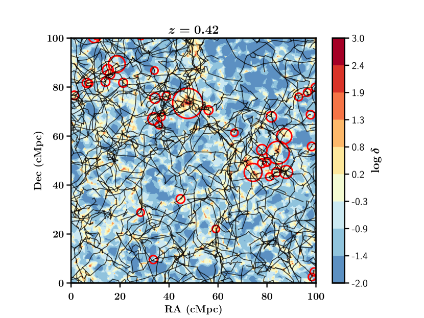
(a)

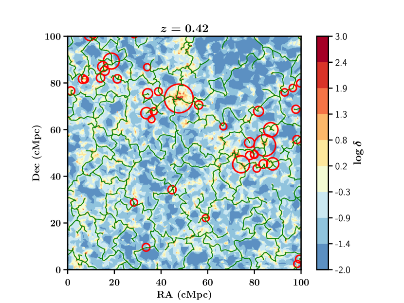
(b)

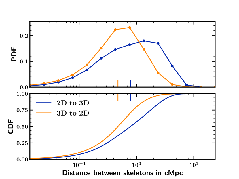
(c)

Figure 1: Top: $100\times 100$ cMpc part of a slice centered at $z=0.42$ in the mock data. The background distribution $\log\delta$ is the logarithm of the DTFE obtained from the galaxy distribution in the slice (with photo-$z$s). Red circles show the positions of halos in the lightcone with redshifts $0.41<z<0.43$. The radius of the circle is equal to $2\times R_{200}$ for display purposes. In panel (a) black lines are the 3D projected skeleton. In panel (b) green lines are the 2D skeleton.
Bottom: Distribution of the distances between skeletons. The distance from the 2D skeleton to the 3D (projected) skeleton is shown in yellow. The distance from the 3D (projected) skeleton to the 2D skeleton is shown in blue. The top panel shows the Probability Distribution Function (PDF) and the bottom panel shows the Cumulative Distribution Function (CDF). The vertical lines and associated error bars on the top panel are the median and error on the median of each distribution.

2.3.2 3D cosmic web extraction

Here, the 3D skeleton extraction is performed on the Merson et al. (2013) lightcone with DISPERSE. As will be detailed in Sect. 3, this is done to assess the reliability of the 2D reconstruction.

Ideally, one would like to compare the 2D reconstruction to a reference skeleton obtained from the dark matter (DM) particle distribution in the lightcone, as galaxies are a biased tracer of the underlying DM distribution (see e.g. Laigle et al., 2018, for a discussion). Here we chose to work with a lightcone with a large FoV in order to have meaningful statistics regarding filaments around clusters of different masses, and to be able to trace filaments on large scales. The chosen lightcone (Merson et al., 2013) only allows to access the mock galaxy distribution. However, since this work does not focus on quantifying the bias of using galaxies as a tracer of the cosmic web, but rather on the ability to recover the 3D density field obtained from galaxies with photometric redshifts, this choice is not penalising. Moreover, reconstruction of the cosmic web from the galaxy distribution in 3D has been shown to trace underlying properties of the density field and its specific geometry (see e.g. Malavasi et al., 2017; Kraljic et al., 2018).

To choose our reference skeleton there are two parameters that we need to tune. Indeed, as explained in Sect. 2.3.1, the skeleton is going to change as the detection threshold is modified. It also depends on the stellar mass limit of the sample used. Up to $z=1$ the Merson et al. (2013) lightcone is complete down to $M_{*}\sim 2.5\times 10^{8}\ {\rm M_{\odot}}$.

The aim of this work is to detect and study filaments of galaxies around galaxy clusters based on photometric redshifts. As detailed in Sect. 2.3.3, the photometric redshift uncertainty prevents us from detecting the leafs and leaflets of the cosmic web. We thus need to choose both the stellar mass and the significance cut in 3D appropriately, to allow for a meaningful comparison.

Working only with the most massive galaxies, we might miss some fainter filaments, but decreasing the mass limit will include more faint filaments that we will not be able to recover in 2D. For our reference 3D skeleton, we chose to work with a stellar mass cut $M_{*}>10^{9}\ {\rm M_{\odot}}$ and a significance threshold set to $5.5\sigma$. We checked on sub-samples of the mock data that our results are not too sensitive to the exact choice of these parameters.

2.3.3 2D cosmic web extraction

To identify cosmic filaments in the CFHTLS from photometric redshifts, we apply the method outlined in Laigle et al. (2018), with two main modifications.

As in Laigle et al. (2018), the galaxy catalogue is cut along the redshift dimension in slices of constant co-moving size. This ensures that the quality of the cosmic web reconstruction is the same at all redshifts and thus avoids possible systematics due to increased slice thickness at higher redshifts.

Galaxies belong to the slice corresponding to their photo-$z$. To compute the density field in 2D from these galaxies, we use the DTFE in two dimensions, each galaxy being weighted by its probability to be in the slice $p_{\rm gal,slice}$ :

$$\left.p_{\rm gal,\ slice}=\int_{z_{\rm inf}}^{z_{\rm sup}}P_{\rm gal}(z)\ dz\ \middle/\int_{0}^{\infty}P_{\rm gal}(z)\ dz\right.$$ (5)

where $z_{\rm inf},z_{\rm sup}$ are the limits of the redshift slice.

To deal with boundary conditions, we add a surface of “guard particles” outside the bounding box by interpolating the actual density at the boundary. Galaxies in masked areas are removed from the catalogue. We do not fill these regions with fake particles as can sometimes be done (e.g. Aragon-Calvo et al., 2015). Once the density is computed we extract the skeleton using DISPERSE with a persistence threshold of $2\sigma$ as in Laigle et al. (2018). The main modifications of the method in this work are:

$\bullet$ Galaxies in each slice are selected following an absolute magnitude cut rather than a stellar mass cut as in Laigle et al. (2018). Here, we select galaxies with $m_{i}<m^{*}_{i}(z)+1.5$, where $m^{*}_{i}(z)$ is computed using Bruzual & Charlot (2003) single stellar population models calibrated with the field galaxy luminosity function (GLF) of Ramos et al. (2011). This cut ensures a good sampling while limiting the photo-$z$ uncertainty.

$\bullet$ Since our study focuses on cosmic filaments around galaxy clusters, the centring of the slices is different. Here, the skeleton around each cluster is reconstructed from a slice centred at the cluster redshift. This ensures an optimal reconstruction as the bias from photo-$z$s is minimised.

3 Validation of the connectivity measurement/filament extraction on mocks

The aim of this section is to quantify the ability of photo-$z$s to trace accurately the cosmic web in the CFHTLS data. Laigle et al. (2018) showed that high quality photo-$z$s from Laigle et al. (2016) in the COSMOS survey (Scoville et al., 2007) allow to probe the cosmic web influence on galaxies up to high redshift ($z\sim 0.9$). Their sample has a typical photo-z uncertainty of $\sigma_{z}=0.008\times(1+z)$ at $z<0.9$.

The photo-$z$ uncertainty in the CFHTLS is $\sim 0.03\times(1+z)$ (at $m_{i}<m^{*}_{i}(z)+1.5$, $z<0.7$). As the photo-z uncertainty drives the slice width, in the CFHTLS slices are chosen to be thicker than in COSMOS. We chose a fixed width of 300 comoving Mpc (cMpc) in the CFHTLS rather than 75 cMpc in COSMOS (Laigle et al., 2018). This choice is justified in Table 1. Considering the increased slice width, we needed to ensure that applying the Laigle et al. (2018) method to the CFHTLS data allowed to obtain a fair reconstruction of cosmic filaments around clusters.

To do so we worked on our modified CFHTLS-like (Merson et al., 2013) lightcone to test the quality of the skeleton reconstruction with CFHTLS-like photo-$z$s. Once the slices were chosen, we applied the method described in Sect. 2.3.3 to extract the skeleton at the $2\sigma$ level. We first considered the global skeleton reconstruction in the slice as in Laigle et al. (2018) (Sect. 3.1). We then focused on the reconstruction around clusters studying the connected filaments (Sect. 3.2)

$z$	$m_{i}^{*}+1.5$	$\sigma_{z}$	$W_{\rm com}$
$0.10<z<0.20$	18.40	0.040	308.6
$0.20<z<0.30$	19.60	0.035	258.7
$0.30<z<0.40$	20.45	0.036	254.1
$0.40<z<0.50$	21.05	0.039	261.8
$0.50<z<0.60$	21.65	0.045	282.2
$0.60<z<0.70$	22.15	0.050	299.5
$0.70<z<0.80$	22.65	0.072	412.0

Table 1: Redshift uncertainties $\sigma_{z}$ and how they drive the choice of the slice thickness. $W_{\rm com}$ is the co-moving width ($\pm\sigma_{z}$) in co-moving Mpc (cMpc) and $m_{i}^{*}$ the typical apparent knee magnitude of the field Galaxy Luminosity Function (GLF). See text for details.

3.1 Global skeleton

3.1.1 Distances between skeletons

To quantify the quality of the photometric reconstruction in the CFHTLS, we computed the distribution of the distances between the segments of the 2D skeleton and the projected 3D skeleton (Sousbie et al., 2008). This is done by computing, for each segment of the 2D skeleton, the minimum distance to a segment of the 3D skeleton. This operation can be reversed to compute the distance of the projected 3D skeleton to the 2D skeleton.

Following Laigle et al. (2018), we define the purity as the proportion of 2D segments that are closer than $1.5\ {\rm cMpc}$ from a projected 3D segment. Inversely, the completeness is the proportion of projected 3D segments that are closer than $1.5\ {\rm cMpc}$ from a 2D segment.

The results are summarised in Table 2, where we give the completeness and the purity as well as the median of the distribution of distances. The full distributions of the distances are shown in Fig. 1(c).

	Completeness	Purity	median (2D -¿ 3D)	median (3D -¿ 2D)
Global skeleton	0.70	0.91	$0.48_{-0.32}^{+0.66}$	$0.79_{-0.58}^{+1.56}$
Filaments connected to clusters	0.71	0.66	$0.73_{-0.63}^{+2.79}$	$0.41_{-0.34}^{+3.40}$

Table 2: Statistics of the distances between the 2D and 3D skeletons detected at $2\sigma$ and $5.5\sigma$ respectively. Quoted uncertainties encompass 68% of the PDF. See text for details.

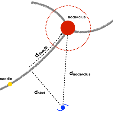
Figure 2: Schematic view of the cosmic web as traced by DISPERSE that defines the different distances used in this chapter. The grey lines are the filaments. The red and yellow points are respectively a node and saddle point. The red dashed circle shows the exclusion radius around the node. $d_{\rm skel}$ is the distance to the skeleton, $d_{\rm node/clus}$ the distance to the node and $d_{\rm clus,fil}$ the distance to the cluster along the filament.

We note that with the thresholds chosen in 3D ($5.5\sigma$) and in 2D ($2\sigma$), when the 3D skeleton is projected in the redshift slices, there are about twice as many 3D projected filaments than 2D filaments. This should impact our selection function by biasing results towards higher purity and lower completeness compared with the case where $N_{\rm fil,2D}\equiv N_{\rm fil,3D}$. Yet, when choosing a higher significance threshold in 3D, from visual inspection, it was clear that some filaments having a counterpart at $5.5\sigma$ were considered as false detections, thus biasing our purity towards lower values.

3.1.2 Stellar mass gradients towards filaments

We have shown that the 2D skeleton is a good tracer of the projected 3D structures. However, to use the 2D skeleton in real data to infer filament properties we need to confirm that we can trace signals that actually exist in 3D from our reconstruction. Here, we consider the stellar mass gradient towards filaments observed in 3D by Malavasi et al. (2017) and Kraljic et al. (2018). Laigle et al. (2018) showed that this gradient is recovered by the 2D reconstruction given the COSMOS precision. Here, we study whether it is recovered in our CFHTLS-like mock or not.

As in Laigle et al. (2018) and Kraljic et al. (2018) we remove the contribution of nodes by removing galaxies too close to nodes, in order to compute the effect of filaments alone. Indeed, there is a known stellar mass gradient towards nodes (i.e. clusters and groups) that we do not want to account for here. Therefore, we stress that the stellar mass gradients we detect are valid at a given scale.
Stellar mass gradients are measured in three stellar mass bins: $9.5<\log{M_{*}/M_{\odot}}\leq 10$, $10<\log{M_{*}/M_{\odot}}\leq 11$ and $11<\log{M_{*}/M_{\odot}}\leq 12$. In each bin, we measured the distance of all galaxies to their closest filaments as illustrated in Fig. 2.

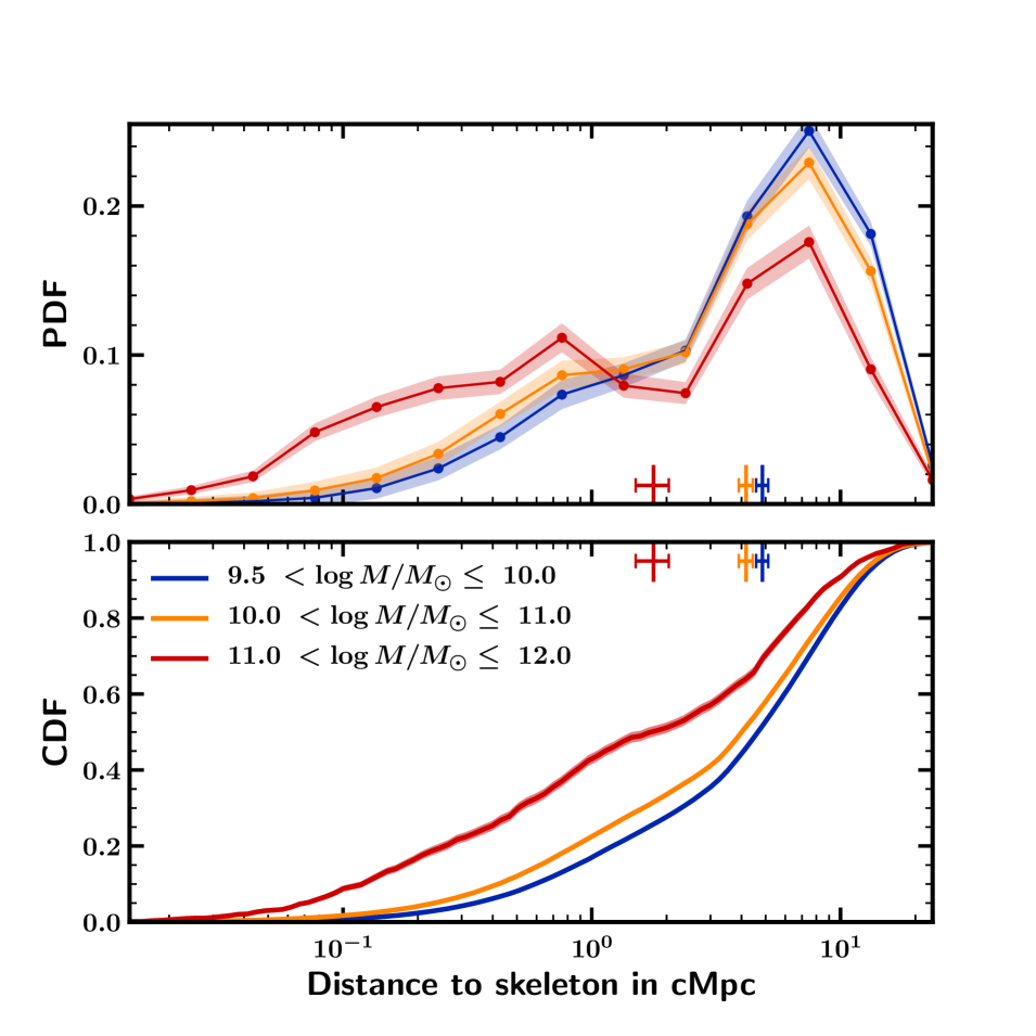
(a) 3D at $5.5\sigma$

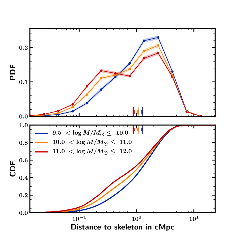
(b) $\sigma_{0}=0.03$

Figure 3: Stellar mass gradients towards filaments detected in 3D and in 2D using the mock data. We split the galaxy catalogue in three mass bins for which we compute the distribution of the galaxy distances to the skeleton after having removed galaxies close to nodes (see text for details). Red is for $11<\log M_{*}/M_{\odot}<12$, yellow for $10<\log M_{*}/M_{\odot}<11$ and blue for $9.5<\log M_{*}/M_{\odot}<10$. In each subfigure, the top distribution is the PDF of the distances to the skeleton. The filled areas around the curves represent the 68% confidence limits computed from 10000 bootstrap re-samplings of the distributions. The bottom panels show the CDF. The vertical lines and associated error bars are the median and error on the median of each distribution.

In 3D, we remove all galaxies that are closer than 3.5 cMpc from a node. This is a rather conservative choice. Indeed, this value is larger than $\sim 2R_{200}$ for the most massive halo in the lightcone. We take the $5.5\sigma$ skeleton as our reference skeleton for the 3D measurement. We tested that when lowering the significance threshold the distances of galaxies to filaments increase as fainter groups are classified as nodes and thus removed. The inverse is true when increasing the detection threshold, as the less massive halos are not detected any more, so their galaxies are included in the distance to filament statistics.The results are shown in Fig. 3. A significant stellar mass gradient towards filaments is detected in 3D, with more massive galaxies lying closer to filaments.
In 2D, we adopt a projected exclusion radius of 1 cMpc. This is less conservative. Yet, adopting a larger value would drastically reduce the available statistics, while a smaller radius increases the influence of the nodes in the measurement, making the 1 cMpc choice a good compromise. The results are presented in Fig. 3. The stellar mass gradient towards filaments can still be observed in 2D even though it is dimmed compared to the 3D signal.

Median values of the PDF (in cMpc)
$\log M_{*}$	3D	2D mock data
$9.5<\log{M_{*}/M_{\odot}}<10$	$4.37\pm 0.02$	$1.26\pm 0.01$
$10<\log{M_{*}/M_{\odot}}<11$	$3.77\pm 0.02$	$1.09\pm 0.01$
$11<\log{M_{*}/M_{\odot}}<12$	$1.51\pm 0.22$	$0.88\pm 0.03$

Table 3: Median values of the galaxy distances to the skeleton in three mass bins, in the original 3D lightcone and in the three toy-model mocks considered in this work. Error bars are the error on the median computed from 100 bootstrap re-samplings of the original distribution. Values are in cMpc.

The median values of the PDF for the different mass bins and different cases are reported in Table 3.

3.2 Reconstruction around clusters

3.2.1 Cluster connectivity

The quality of the reconstruction in the infall regions of clusters can also be assessed by studying the cosmic connectivity $\kappa$ of clusters at the nodes of the cosmic web, i.e. the number of cosmic filaments connected to a cluster.

Cosmic connectivity is expected to scale with cluster mass, more massive clusters being more connected (see e.g. Aragón-Calvo et al., 2010; Gouin et al., 2017; Codis et al., 2018; Darragh Ford et al., in prep), though with large intrinsic scatter (see in particular Aragón-Calvo et al., 2010). Finding such a correlation from our 2D filaments would give an independent confirmation of our skeleton reconstruction quality, particularly in cluster infall regions.

In the lightcone, we computed the connectivity considering the 3D skeleton. The same measurement was carried out in our CFHTLS-like mock data using the 2D reconstruction.

In the skeleton extracted with DISPERSE, all nodes are linked to one or several saddle-points through filaments such that one node may be connected to several filaments. Formally, in the skeleton extracted by DISPERSE, two filaments leading to the same node can become infinitely close but still be counted separately, as they are both topologically robust. However, they represent only a single filament physically speaking. Thus to avoid double counting, these are merged into a single filament and a bifurcation point is added where they diverge. Our measure of a node’s connectivity is then the number of physical filaments departing from the node and crossing the sphere (3D) or circle (2D) of radius $1.5$ cMpc centred on the node. This definition is slightly different from that of Darragh Ford et al. (in prep) where they took a radius of $1.5\times R_{200}$. This is because our CFHTLS candidate cluster mass estimate has a high uncertainty ($\sim 0.20-0.25\ {\rm dex}$) compared to theirs. Using the value of $R_{200}$ computed from our estimated $M_{200}$ would thus introduce noise in our connectivity measurement.

To compute the number of filaments connected to a given cluster, we first match the cluster to the nodes detected by DISPERSE and choose the node which is closest to the cluster. If no node is found at a distance smaller than the cluster $R_{200}$, the cluster is marked as unmatched and not considered in the analysis. Here $R_{200}$ is computed from the halo mass $M_{200}$ following:

$$R_{200}=\left(\frac{3\,M_{200}}{4\pi\,200\,\rho_{c}(z)}\right)^{\frac{1}{3}}$$ (6)

We then define the connectivity of a given cluster as the connectivity of the node it was matched with.

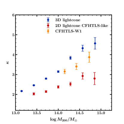
Figure 4: Mean connectivity $\kappa$ in bins of halo mass $\log M_{200}$ in 3D in the Merson et al. (2013) lightcone (blue), and 2D in the CFHTLS-like mock (red) and in the CFHTLS (yellow). Error bars are standard errors on the mean.

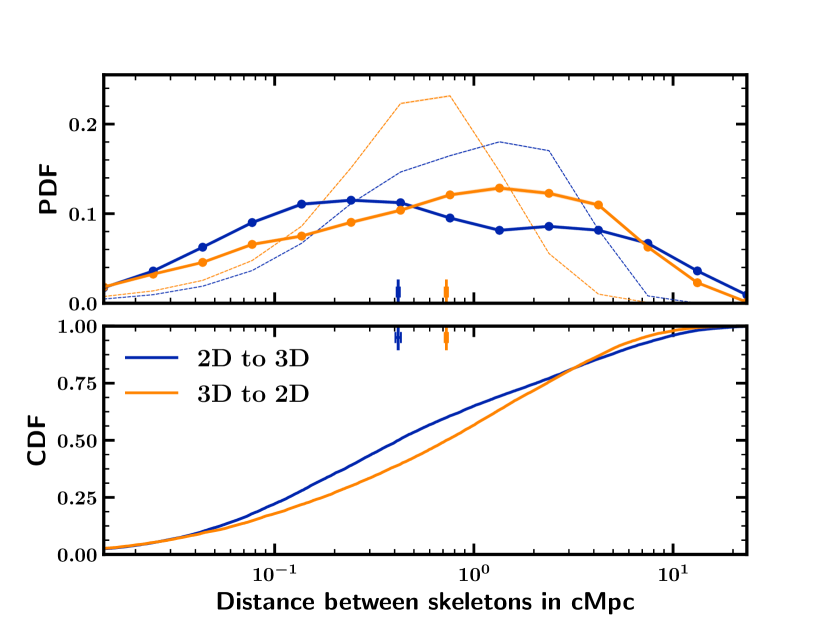
Figure 5: Left: Zoom on the most massive halo in the mock. The red circle shows the radius used to compute the connectivity ($1.5$ cMpc). We show only the filaments of the skeleton connected to the cluster according to the 3D reconstruction (black) and 2D reconstruction (green).The background distribution $\log\delta$ is the logarithm of the DTFE obtained from the galaxy distribution in the slice (with photo-$z$s). Right: Distribution of the distances between skeletons. Solid lines show the distribution for the filaments connected to clusters ($M_{200}>10^{14}M_{\odot}$). The distribution for the global skeleton is shown in the background as thin transparent lines. The top panel shows the PDF and the bottom panel shows the CDF. The vertical lines and associated error bars on the top panel are the median and error on the median of each distribution.

The expected increase of connectivity with cluster mass is recovered as seen in Fig. 4. Error bars are the standard error on the mean. The standard deviation of the distribution in each bin is actually much larger, due to a large intrinsic scatter in the $\kappa-\log M_{200}$ scaling relation. We performed a Spearman correlation test to formally check for correlation between connectivity and mass. In each case, we found a weak but strongly significant correlation. Results are reported in Table 4.

	$r_{s}$	$p-$value
3D mock data	$0.29$	$<<10^{-15}$
2D CFHTLS-like mock data	$0.14$	$<10^{-11}$
CFHTLS-W1	$0.17$	$<10^{-4}$

Table 4: Results of the Spearman correlation test for $\kappa$ vs $M_{200}$ in the three cases studied : 3D mock data, 2D CFHTLS-like mock data and CFHTLS-W1 respectively.

This comparison highlights that the 2D connectivity is biased towards lower values compared to the 3D connectivity. This could come from the fact that some of the 3D filaments are along the line of sight and cannot be recovered in 2D. This could also be due to faint filaments getting blurred into the noise (due either to the slice thickness or to the photo-$z$ uncertainty). Moreover, this test seems to indicate that the bias is slightly dependent on halo mass, the slopes of the 2D and 3D scaling relations being different.

We note that in both cases we did not find any redshift evolution of the connectivity in the range $0.1<z<0.7$. This is compatible with measures by Codis et al. (2018), where only a weak evolution is found between $z=0$ and $z=1.3$.

3.2.2 Distance between skeletons in cluster infall regions

To go beyond connectivity and check if the 2D cosmic filaments connected to clusters are representative of the 3D connected cosmic filaments, we computed the distances between these filaments in the mocks. This allows to check if their directions statistically agree, which could not be assessed from the connectivity measurement.

The extraction of connected filaments is done as in Sect. 3.2.1. The distances between the 3D and 2D connected filaments are computed as in Sect. 3.1.1. Results are displayed in Fig. 5.

The median of distances between 2D and 3D filaments is higher with this method than when comparing the global skeletons (see Fig. 1(c)). This is due to projection effects existing in the global method, as some filaments that may be in the background or in the foreground and thus not connected to the clusters are included in the global reconstruction. Our results are not affected by these projections here. On the other hand, the median of distances between 3D and 2D filaments is lower, as fewer 3D filaments have no counterpart in 2D.

This reflects in the purity of the reconstructed filaments (computed as in Sect. 3.1.1, matching segments closer than 1.5 cMpc). Indeed this drops to 66%, meaning that around two thirds of the reconstructed connected filaments correspond to actual 3D filaments feeding the clusters. The analysis of Sect. 3.1.1 then indicates that about 20% of reconstructed filaments correspond to 3D filaments appearing in the slice because of projection effects, and 10% are just false detections due to projection effects in the galaxy distribution and photometric redshift errors. On the other hand, the reconstruction allows to detect $\sim 70\%$ of true 3D connected filaments.

3.3 Caveats and limitations of the method

One major limitation of our reconstruction method is obviously the fact that, as we work in 2D we are sensitive to projection effects. If DISPERSE deals with Poisson noise and should thus clean properly spurious alignments, our results may be affected by coherent projection effects due to walls or filaments oriented in the direction of the slicing. The former might then be detected as a filament and the latter as a node.

The amplitude of this effect is difficult to quantify, but it might play a role when computing the stellar mass gradient towards filaments in 2D. Indeed, it can be seen in Fig. 3 that the behaviours in 3D and 2D are not the same. Massive galaxies in the 3D skeleton present a pronounced gradient that does not appear as clear in 2D. This may be due to the fact that, as Kraljic et al. (2018) showed, in addition to the stellar mass gradient towards filaments, there is also a stellar mass gradient towards walls as well, that we pick up in our 2D analysis.

Despite this limitation, we reach a quite high purity in our 2D filament detection at the CFHTLS accuracy ($\sim 90\%$ in the global skeleton reconstruction and $\sim 70\%$ for filaments connected to clusters). We can thus use our filament reconstruction on the CFHTLS T0007 data to study how filaments impact galaxy properties.

4 Cosmic filaments around AMASCFI clusters in the CFHTLS

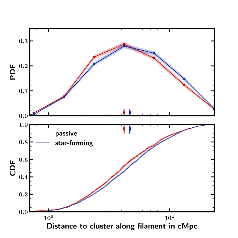
(a) $0.15<z\leq 0.4$

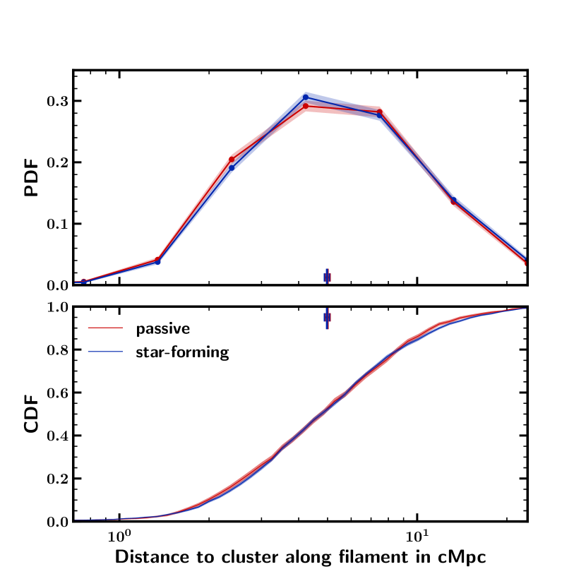
(b) $0.4<z<0.7$

Figure 6: Distances to AMASCFI clusters along filaments of passive galaxies (red) and star-forming galaxies (blue) respectively at low (a) and high (b) redshifts. The top distribution is the PDF of the distances to the skeleton. The filled areas around the curves represent the 68% confidence limits computed from 100 bootstrap re-samplings of the distribution. The significance of the difference between the passive and star-forming galaxy distributions is written at each sampling point. The vertical lines and associated error bars are the median and error on the median of each distribution.
The bottom panel shows the CDF.

We then proceeded to study the properties of cosmic filaments around AMASCFI clusters in the CFHTLS T0007 data. We particularly focused on the role filaments may play in environmental quenching by pre-processing galaxies infalling in galaxy clusters, by comparing the properties of passive and star-forming galaxies. To this aim, we reconstructed the filaments using the technique described in Sect. 2.3.3. The ability of this technique to statistically trace the true 3D cosmic web at the CFHTLS precision was demonstrated in Sect. 3.

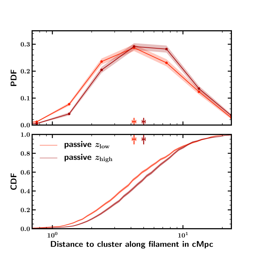
(a) passive galaxies

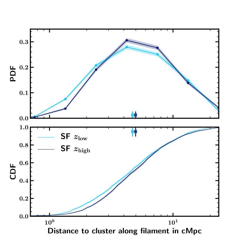
(b) star-forming galaxies

Figure 7: Distances to AMASCFI clusters along filaments of respectively passive galaxies (a) and star-forming galaxies (b) at high (dark) and low (light) redshift. See Fig. 6 for details on symbols.

Median values of the PDF (in cMpc)
	passive galaxies	star-forming galaxies	$\Delta_{{\rm passive}-{\rm star-forming}}$
$0.15<z_{clus}<0.70$	$4.50\pm 0.05$	$4.98\pm 0.05$	$7.6\sigma$
$0.15<z_{clus}\leq 0.40$	$4.22\pm 0.08$	$4.71\pm 0.07$	$4.9\sigma$
$0.40<z_{clus}<0.70$	$5.00\pm 0.13$	$4.98\pm 0.10$	NS
	$----$	$----$
$\Delta_{z_{\rm low}-z_{\rm high}}$	$5.0\sigma$	$2.3\sigma$

Table 5: Median values of the PDF of the filament galaxy distances to AMASCFI clusters along filaments for passive galaxies and star-forming galaxies in different redshift bins. NS stands for ’not significant’ and $\Delta_{X-Y}$ is defined in eq. 7

4.1 Galaxy cluster connectivity

To compute the connectivity of AMASCFI clusters, we used the same method as in Sect. 3.2.1. The difference is that here, we do not know the exact position of the cluster but rather its estimate as computed by AMASCFI. So this should introduce some bias in our connectivity measurement. The same is true for the mass. The cluster $R_{200}$ is computed from the AMASCFI mass estimate following eq. 6.

We investigated the scaling between the connectivity and cluster mass in the CFHTLS-W1 field from AMASCFI clusters using three mass bins $14<\log M_{200}/M_{\odot}\leq 14.3$, $14.3<\log M_{200}/M_{\odot}\leq 14.6$, and $\log M_{200}/M_{\odot}>14.6$, as in Sarron et al. (2018).

We do recover the expected connectivity increase with cluster mass as can be seen in Fig. 4 (yellow points). Such a scaling was also found in lower mass groups in the COSMOS survey by Darragh Ford et al. (in prep). In this figure, the error bars are standard errors on the mean. The standard deviation of the distribution in each bin is actually much larger, due to a large intrinsic scatter in the $\kappa-\log M_{200}$ scaling relation. We note that the mean connectivity at a given mass is higher in the CFHTLS data when compared to the value obtained in the lightcone. This could be due to the difference in number counts between the mock and the data mentioned in Sect. 2.

4.2 Galaxy-type gradients towards clusters

Since galaxies fall along filaments onto clusters, we might expect to see a redshift dependence of their median distance to clusters along filaments. If galaxies are quenched inside filaments in their fall towards clusters, we then expect to see a colour-type gradient toward clusters inside filaments.
DISPERSE allows one to carry such a measurement, as for each cluster the connecting filaments are well defined (see Sect. 3.2.1). Moreover we showed in Sect. 3.2.2 that the 2D reconstructed filaments are a good tracer of the actual 3D filaments feeding clusters ($\sim 70\%$ completeness and purity). We can thus compute the distribution of the distances to AMASCFI clusters along their connecting filaments.
Galaxies at a distance $d_{\rm skel}<1\ {\rm cMpc}$ are considered filament members. This definition is coherent with that of Tempel et al. (2014) (who took a radius of $0.5h^{-1}$ (physical) Mpc at $z<0.15$, which corresponds to $1$ cMpc at $z=0.4$) and more restrictive than Martínez et al. (2016) who used a radius of $1.5h^{-1}$ (physical) Mpc at $z<0.15$.

This definition of the comoving radial size is fixed for all filaments connected to the AMASCFI clusters. We plotted the radial profile (without background substraction) of these filaments as a function of several parameters. In particular, we checked the dependency of the radial profile as a function of the cluster redshift, cluster mass $M_{200}$, and distance to the cluster along the filament. We found no redshift evolution nor dependence on cluster mass (no significant difference between the distributions). The radial profiles show no significant variation at $d_{\rm clus,fil}>1.5$ cMpc. At $d_{\rm clus,fil}\leq 1.5$ cMpc, filaments become significantly more concentrated, showing that the influence of the cluster on the filaments becomes significant at this distance only - corresponding roughly to the virial radius.

We computed the distance to the connected cluster along the filament axis $d_{\rm clus,fil}$ for these galaxies. We did not account for $d_{\rm skel}$ in the measurement (see Fig. 2 for the distance definitions). Since we are interested in the role played by cosmic filaments in quenching, we remove all galaxies at a distance $d_{\rm clus}<R_{200}$ from the cluster.

This measurement was done for passive and star-forming galaxies separately. The segregation between the two populations is done using the SED classification given by LePhare at the galaxy best photo-$z$. We also split our cluster sample in two redshift bins $0.15<z\leq 0.4$ and $0.4<z<0.7$ respectively. We note that the classification of galaxies as passive or star-forming using SED fitting with five optical bands is not extremely robust for individual galaxies, as the star-formation rate of galaxies cannot be computed precisely. This may introduce some noise in our measurements.

In the following, we compare the distribution of $d_{\rm clus,fil}$ for the two galaxy populations (passive and star-forming) and redshift bins (low redshift and high redshift). To this aim we give the estimated medians of each distribution and compare them. The formal comparison of the distributions was done by performing a Kolmogorov-Smirnov (KS) test on the CDFs with 10000 bootstraps. For each bootstrap realisation we test the null hypothesis that the samples are drawn from the same parent distribution. The significance of the difference between the samples is then quantified through the fraction of bootstrap realisations for which the null hypothesis is rejected (KS $p-{\rm value}<0.01$).

Results are presented in Fig. 6, where we show the distributions of $d_{\rm clus,fil}$ for passive galaxies and star-forming galaxies in the low (left) and high (right) redshift bins and in Fig. 7, where we show the distributions of $d_{\rm clus,fil}$ for passive galaxies (left) and star-forming galaxies (right) in the two redshift bins. Note that in these two figures, we are displaying the same four distributions but Fig. 6 focuses on the galaxy-type difference at a given redshift, while Fig. 7 focuses on the redshift evolution for a given galaxy type.

We see in Fig. 6 that there is no difference in the distance distribution between passive galaxies and star-forming galaxies at high redshift (the KS null hypothesis cannot be rejected in $\sim 95\%$ of bootstrap resamplings, see Fig. 10(b)). On the other hand, passive galaxies are slightly closer to clusters at low redshift (the KS null hypothesis can be rejected in $\sim 90\%$ of bootstrap resamplings, see Fig. 10(a)). If interpreted in the context of the colour-density relation (e.g. Cooper et al., 2007), the difference at low redshift actually confirms that by applying DISPERSE with photo-$z$s we are able to recover a density increase along filaments up to AMASCFI outside $R_{200}$.

When looking at Fig. 7, we see that both galaxy populations see their distances to clusters along filaments decrease with decreasing redshift, but the trend is stronger for passive galaxies. The difference between the distributions is significant in both cases (the KS null hypothesis can be rejected in $\sim 98\%$ of bootstrap resamplings, see Fig. 11).

Values and differences of the distribution medians are reported in Table 5 where:

$$\Delta_{X-Y}=\frac{\left|d_{X}-d_{Y}\right|}{\sqrt{\sigma_{d_{X}}^{2}+\sigma_{d_{Y}}^{2}}},$$ (7)

whith $d_{X}$ and $d_{Y}$ the distances (or their medians) and $\sigma_{d_{X}}$ and $\sigma_{d_{Y}}$ the associated uncertainties. These results are discussed in Sect. 5.

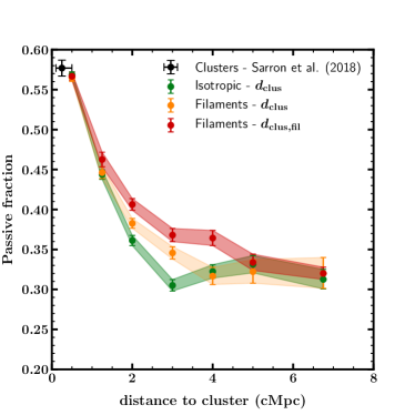
Figure 8: Galaxy passive fraction as a function of the distance to the cluster in comoving Mpc. Red points are galaxies in filaments connected to the clusters, whose clustercentric distance is computed along the filaments. The results for the same galaxy sample but with clustercentric cartesian distance is plotted in yellow. In green we plot galaxies in annuli around the clusters, considered to fall on the cluster isotropically.

4.3 Passive fraction

If quenching is efficient in cosmic filaments, we might expect to see an increased fraction of passive galaxies in their galaxy population compared to the field. To check for this, we computed the passive fraction in filament galaxies. Filament galaxies were selected and split between passive and star-forming galaxies as in Sect. 4.2.

To ensure that we probe the specific effect of cosmic filaments on the passive fraction, we proceeded in a similar way to Martínez et al. (2016). We chose as a reference sample galaxies in the infall region of clusters ($d_{clus}>R_{200}$) but outside filaments. For each cluster, we selected galaxies whose closest projected node in the slice is the cluster and that are not located in filaments ($d_{\rm skel}>1$cMpc). As in Martínez et al. (2016), we refer to these as isotropically falling galaxies or isotropic galaxies. The passive fraction in filaments is found to be $f_{\rm passive,fil}=0.370\pm 0.006$ while the passive fraction of isotropic galaxies is $f_{\rm passive,iso}=0.301\pm 0.007$.

Then, we computed the passive fraction of filament galaxies as a function of their distance to the cluster over the full redshift range $0.15<z<0.7$. Results are shown in red in Fig. 8. Error bars and shaded areas are the 68% confidence intervals for binomial population proportions computed following Cameron (2011). The passive fraction of isotropic galaxies as a function of distance to the cluster is plotted in green.

When we compute the distance to the cluster along the filaments $d_{\rm clus,fil}$, we may introduce a bias compared to the isotropic sample, as filaments wind around on their way to the cluster. Thus, to cancel out this effect, we compute the cartesian distance to the cluster for galaxies in filaments (the yellow points in Fig. 8).

Both for filament galaxies and isotropic galaxies, there is a smooth decrease of the passive fraction as a function of increasing clustercentric distance. The value at $d_{clus}<1$ cMpc is compatible with the passive fraction observed in clusters by Sarron et al. (2018).

The passive fraction remains higher in filaments as the distance from the cluster increases up to $d_{clus}\sim 4-5$ cMpc, which roughly corresponds to $(2.5-3)R_{200}$. The excess of passive galaxies remains between $2$ and $4$ cMpc when considering the cartesian distance to the cluster. These results are discussed in Sect. 5.

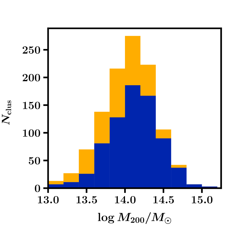
Figure 9: Top: histogram of groups/clusters respectively matched (blue) and unmatched (gold) with DISPERSE nodes, as a function of their $M_{200}$ in the CFHTLS-W1 field. The two histograms are stacked on top of each other so that their sum is the total number of groups/clusters in the mass bin. Bottom: distribution of the distances to the skeleton of groups not located at a node in CFHTLS-W1. The dashed line is the chosen radius for filaments ($r=1$ cMpc). See Fig. 6 for details on symbols.

4.4 Galaxy groups inside filaments

As already mentioned, according to Libeskind et al. (2018), on large scales most filament finders tend to locate groups of $M_{200}\sim 10^{13.5}$ M_⊙ inside cosmic filaments rather than at the nodes of the cosmic web. If groups are indeed located in filaments, then they may play a role in the observed gradient towards clusters observed in Sect. 4.2 and in the passive fraction observed in Sect. 4.3.

As mentioned in Sect 4.1, when computing the connectivity, some halos are not matched to DISPERSE nodes. The proportion of unmatched halos is actually a function of halo mass. This is shown in Fig. 9 where we plot the histogram of matched and unmatched halos as a function of $\log M_{200}/M_{\odot}$ in CFHTLS-W1. We see that most massive clusters are all matched to a node from the skeleton reconstruction. Yet many low mass AMASCFI candidate clusters and groups are not matched to a node.

We thus computed the distances of these unmatched groups to the filaments traced by DISPERSE in order to see where they are located with respect to the filaments of the cosmic web. The distances are computed in two dimensions, in the slice centred at the cluster redshift.

Results are displayed in Fig. 9. Looking at the CDF, we see that more than $75\%$ of groups are located in filaments ($d_{\rm skel}<1\ {\rm cMpc}$). These results have implications on the interpretation we can give to the galaxy-type gradient towards clusters along filaments that we observed in Sect. 4.2 and to the observed passive fraction in filaments observed in Sect. 4.3, as discussed in Sect. 5.

5 Discussion

In Sect. 4.2, we showed that the median distance to clusters along filaments of both passive and star-forming galaxies is slightly higher at high redshift than at low redshift. While the trend is faint, a KS test confirmed that it is significant (see Figs. 10 and 11). This would agree with a picture where galaxies follow filaments towards the cluster potential well in the redshift range $0.15<z<0.7$.

When comparing the distributions of passive and star-forming galaxies in the two redshift bins separately (see Fig. 6), we observed a galaxy type gradient towards clusters inside filaments in the low redshift bin only ($0.15<z_{clus}\leq 0.4$), passive galaxies being located in the regions closer to clusters along filaments than star-forming galaxies. At high redshift ($0.4<z_{clus}<0.7$), the distributions are the same for passive galaxies and star-forming galaxies. So passive galaxies in filaments are located closer to clusters in the low redshift bin but not in the high redshift bin. Again, the trend, while faint, was confirmed to be significant by a KS test.

Moreover, we showed in Sect. 4.3 that over the full redshift range ($0.15<z<0.7$), the fraction of passive galaxies in filaments is higher than in regions around clusters outside of filaments (that we referred to as isotropic regions), and the fraction of passive galaxies in filaments decreases with increasing clustercentric distance. This agrees with the findings of Martínez et al. (2016) at $z<0.15$ and Salerno et al. (2019) at $0.43\leq z\leq 0.89$, while exploring redshifts intermediate between these two studies. This is also in agreement with the findings of Kraljic et al. (2018) in the GAMA survey in the range $0.03\leq z\leq 0.25$ that found that the red fraction depends simultaneously on the distance to the filament and the distance to nodes.
We remind the reader that our results are based on classification of passive and star-forming galaxies using SED fitting. This classification is statistically correct but is not extremely robust for individual galaxies when using five optical bands as it is the case in the CFHTLS. Some galaxies may thus be wrongly classified as passive or star-forming, introducing noise in our galaxy-type gradient and passive fraction measurements.

Finally, we showed in Sect. 4.4 that some low mass clusters and groups in the AMASCFI catalogue are not located at nodes as detected by our skeleton reconstruction. Looking at the distances of these unmatched groups to the skeleton, we found that most of them ($\sim 80\%$) are located in filaments. This is in agreement with the scenario of hierarchical structure formation, in which clusters keep accreting smaller groups in the redshift range $0.15<z<0.7$ (e.g. Contini et al., 2016).

These results can be interpreted in two ways. First, one can assume that passive galaxies fall faster in the potential well that star-forming galaxies. This would explain why passive galaxies are closer to clusters than star-forming ones in the low redshift bin. The increased falling speed could come from a higher radial speed along the filament due to the fact that passive galaxies are located closer to the filament spine (Laigle et al., 2018; Kraljic et al., 2018). One way to understand this is also by thinking of passive galaxies being located preferentially in galaxy groups, that we showed to be mainly located closer to the filament spine and may thus fall faster onto clusters than isolated galaxies. In this case, the fact that we do not observe a significant difference in the distance distributions of passive and star-forming galaxies in our high redshift bin would be coherent with a picture where most of the collapse of groups into clusters occured at $z<0.7$ (Contini et al., 2016).

On the other hand, the results can also be interpreted by quenching occurring in the filaments. This would require that the quenching mechanism is more efficient when galaxies in the filament are located closer to the cluster. This could fit with a scenario where during their journey along the filaments, galaxies have a higher probability to collide or enter a group as satellites, and even more so when they get closer to the cluster. Both phenomena (merger and group accretion) are known to be responsible for quenching. Moreover, in our redshift range, filaments keep accreting field galaxies from the walls/voids in the saddle point regions. As most of these galaxies should be star-forming (e.g. Kraljic et al., 2019), this would tend to increase the median distance of star-forming galaxies to clusters.

In this second scenario, even though our results cannot assess which physical processes might be at play in the filament quenching, it is interesting to note that we also showed that we found groups located close to the filament spines. This could point towards filament quenching being due to pre-processing by galaxy groups through strangulation as argued by De Lucia et al. (2012) or Peng et al. (2015). Yet we lack conclusive evidence to draw firm conclusions and this calls for further investigation.

6 Conclusions

We presented a method to detect the cosmic web filaments based on photometric redshifts. We showed the ability of the method, already applied to the COSMOS field by Laigle et al. (2018), to statistically reconstruct the filament distribution. In particular, we focused here on the infall regions around clusters, where we showed that the scaling of connectivity with cluster mass is recovered, and found a completeness of $\sim 70\%$ and a purity of $\sim 66\%$ for the connected filament reconstruction.

We then applied the method to the CFHTLS T0007 data to study filaments of galaxies around AMASCFI clusters (Sarron et al., 2018). For each cluster, we analysed the cosmic filaments connected to the clusters.

Studying galaxy properties in these filaments connected to clusters, we find that galaxies are located closer to clusters in the redshift range $0.15<z\leq 0.4$ compared to $0.4<z<0.7$. In the low redshift bin, we observed a galaxy-type gradient towards clusters, i.e. passive galaxies are located closer to clusters than star-forming galaxies. Such a gradient does not exist in our high redshift bin. In the full redshift range, we showed that the fraction of passive galaxies is higher in our filaments than in istropically selected regions around clusters and that the passive fraction in filaments decreases with increasing distance to the cluster up to $d_{\rm clus}\sim 5$ cMpc.

We proposed that this could be interpreted as quenching occuring in the filaments before galaxies reach the cluster virial radius - so-called pre-processing. As we found that a large fraction of groups not located at the nodes of the reconstructed cosmic web are in fact inside filaments ($80\%$ of groups at $d_{{\rm skel}}<1$ cMpc), we postulated that this pre-processing could occur in galaxy groups during the hierarchical growth of structures in agreement with previously proposed quenching models (e.g. Wetzel et al., 2013; Moutard et al., 2018).

We plan on building upon this proof-of-concept study by stuying the passive and star-forming galaxy luminosity functions (GLF) of our filaments. This will enable us to better interpret the trends observed in the cluster GLFs and to pinpoint the physical processes at play in quenching star-formation in dense environments.

This method is promising as it uses photometric redshifts of accuracy typical of what is expected for future wide surveys such as Euclid and LSST, that will allow to explore cosmic filaments at even higher redshifts with more statistics.

Appendix A KS tests on distance distributions

As mentioned in Sect. 4.2, to check if the distributions of distances to clusters of galaxies in filaments are different for passive and star-forming galaxies in the low ($0.15<z\leq 0.4$) and high ($0.4<z<0.7$) redshift bins, we performed Kolmogorov-Smirnoff (KS) tests on 10000 bootstrap realisations of the samples. The same was done for passive and star forming galaxies.

The distributions of the $p-$values of these KS tests are presented in Figs. 10 and Fig. 11.

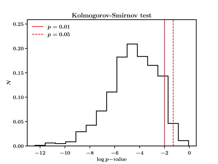
(a) $0.15<z<0.4$

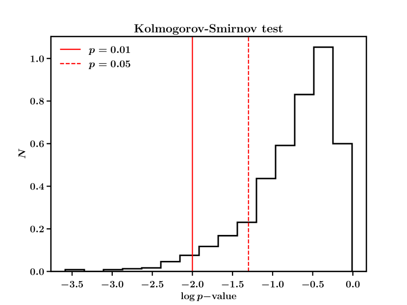
(b) $0.4<z<0.7$

Figure 10: $p-$value histograms of 10000 bootstrap realisations of KS tests on the distributions of Fig. 6 at low (a) and high (b) redshifts respectively.

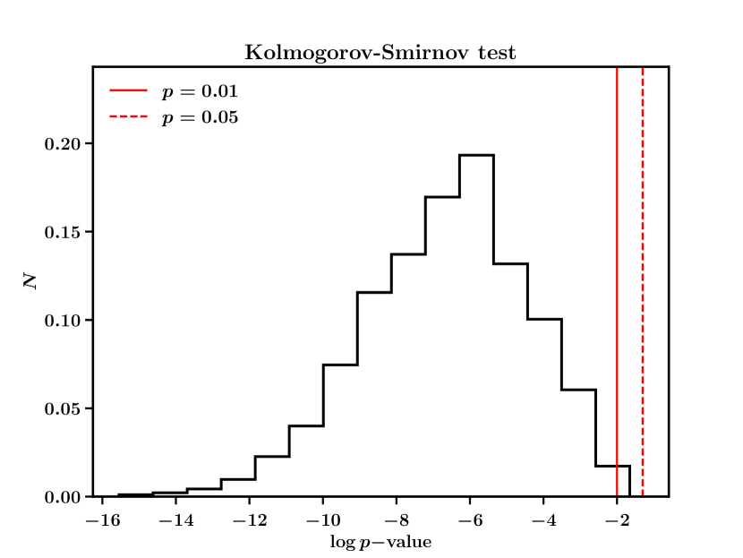
(a) passive galaxies

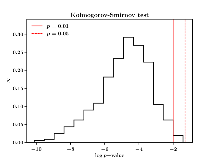
(b) star-forming galaxies

Figure 11: $p-$value histograms of 10000 bootstrap realisations of KS tests on the distributions of Fig. 7 for passive (a) and star-forming (b) galaxies respectively.

References

- Adami et al. (2010) Adami, C., Durret, F., Benoist, C., et al. 2010, A&A, 509, A81
- Aragón-Calvo et al. (2010) Aragón-Calvo, M. A., van de Weygaert, R., & Jones, B. J. T. 2010, MNRAS, 408, 2163
- Aragon-Calvo et al. (2015) Aragon-Calvo, M. A., van de Weygaert, R., Jones, B. J. T., & Mobasher, B. 2015, MNRAS, 454, 463
- Arnouts et al. (1999) Arnouts, S., Cristiani, S., Moscardini, L., et al. 1999, MNRAS, 310, 540
- Baldry et al. (2004) Baldry, I. K., Glazebrook, K., Brinkmann, J., et al. 2004, ApJ, 600, 681
- Bamford et al. (2009) Bamford, S. P., Nichol, R. C., Baldry, I. K., et al. 2009, MNRAS, 393, 1324
- Bianconi et al. (2018) Bianconi, M., Smith, G. P., Haines, C. P., et al. 2018, MNRAS, 473, L79
- Bond et al. (1996) Bond, J. R., Kofman, L., & Pogosyan, D. 1996, Nature, 380, 603
- Bruzual & Charlot (2003) Bruzual, G. & Charlot, S. 2003, MNRAS, 344, 1000
- Cameron (2011) Cameron, E. 2011, PASA, 28, 128
- Castignani & Benoist (2016) Castignani, G. & Benoist, C. 2016, A&A, 595, A111
- Cautun & van de Weygaert (2011) Cautun, M. C. & van de Weygaert, R. 2011, The DTFE public software: The Delaunay Tessellation Field Estimator code, Astrophysics Source Code Library
- Chen et al. (2017) Chen, Y.-C., Ho, S., Mandelbaum, R., et al. 2017, MNRAS, 466, 1880
- Codis et al. (2018) Codis, S., Pogosyan, D., & Pichon, C. 2018, MNRAS, 479, 973
- Coleman et al. (1980) Coleman, G. D., Wu, C.-C., & Weedman, D. W. 1980, ApJS, 43, 393
- Colless et al. (2001) Colless, M., Dalton, G., Maddox, S., et al. 2001, MNRAS, 328, 1039
- Contini et al. (2016) Contini, E., De Lucia, G., Hatch, N., Borgani, S., & Kang, X. 2016, MNRAS, 456, 1924
- Cooper et al. (2007) Cooper, M. C., Newman, J. A., Coil, A. L., et al. 2007, MNRAS, 376, 1445
- Coupon et al. (2009) Coupon, J., Ilbert, O., Kilbinger, M., et al. 2009, A&A, 500, 981
- Darragh Ford et al. (in prep) Darragh Ford, E., Laigle, C., Gozalisal, G., et al. in prep, MNRAS
- de Lapparent et al. (1986) de Lapparent, V., Geller, M. J., & Huchra, J. P. 1986, ApJ, 302, L1
- De Lucia et al. (2012) De Lucia, G., Weinmann, S., Poggianti, B. M., Aragón-Salamanca, A., & Zaritsky, D. 2012, MNRAS, 423, 1277
- Eisenhardt et al. (2008) Eisenhardt, P. R. M., Brodwin, M., Gonzalez, A. H., et al. 2008, ApJ, 684, 905
- Fujita (2004) Fujita, Y. 2004, PASJ, 56, 29
- Gouin et al. (2017) Gouin, C., Gavazzi, R., Codis, S., et al. 2017, A&A, 605, A27
- Gozaliasl et al. (2014) Gozaliasl, G., Finoguenov, A., Khosroshahi, H. G., et al. 2014, A&A, 566, A140
- Guzzo et al. (2014) Guzzo, L., Scodeggio, M., Garilli, B., et al. 2014, A&A, 566, A108
- Hilton et al. (2009) Hilton, M., Stanford, S. A., Stott, J. P., et al. 2009, ApJ, 697, 436
- Ilbert et al. (2006) Ilbert, O., Arnouts, S., McCracken, H. J., et al. 2006, A&A, 457, 841
- Kinney et al. (1996) Kinney, A. L., Calzetti, D., Bohlin, R. C., et al. 1996, ApJ, 467, 38
- Kraljic et al. (2018) Kraljic, K., Arnouts, S., Pichon, C., et al. 2018, MNRAS, 474, 547
- Kraljic et al. (2019) Kraljic, K., Pichon, C., Dubois, Y., et al. 2019, MNRAS, 483, 3227
- Kurk et al. (2009) Kurk, J., Cimatti, A., Zamorani, G., et al. 2009, A&A, 504, 331
- Kuutma et al. (2017) Kuutma, T., Tamm, A., & Tempel, E. 2017, A&A, 600, L6
- Laigle et al. (2016) Laigle, C., McCracken, H. J., Ilbert, O., et al. 2016, ApJS, 224, 24
- Laigle et al. (2018) Laigle, C., Pichon, C., Arnouts, S., et al. 2018, MNRAS, 474, 5437
- Le Fèvre et al. (2005) Le Fèvre, O., Vettolani, G., Garilli, B., et al. 2005, A&A, 439, 845
- Libeskind et al. (2018) Libeskind, N. I., van de Weygaert, R., Cautun, M., et al. 2018, MNRAS, 473, 1195
- Malavasi et al. (2017) Malavasi, N., Arnouts, S., Vibert, D., et al. 2017, MNRAS, 465, 3817
- Malavasi et al. (2016) Malavasi, N., Pozzetti, L., Cucciati, O., Bardelli, S., & Cimatti, A. 2016, A&A, 585, A116
- Martinet et al. (2017) Martinet, N., Durret, F., Adami, C., & Rudnick, G. 2017, A&A, 604, A80
- Martínez et al. (2016) Martínez, H. J., Muriel, H., & Coenda, V. 2016, MNRAS, 455, 127
- Mei et al. (2006) Mei, S., Holden, B. P., Blakeslee, J. P., et al. 2006, ApJ, 644, 759
- Merson et al. (2013) Merson, A. I., Baugh, C. M., Helly, J. C., et al. 2013, MNRAS, 429, 556
- Mirkazemi et al. (2015) Mirkazemi, M., Finoguenov, A., Pereira, M. J., et al. 2015, ApJ, 799, 60
- Moutard et al. (2018) Moutard, T., Sawicki, M., Arnouts, S., et al. 2018, MNRAS, 479, 2147
- Mullis et al. (2005) Mullis, C. R., Rosati, P., Lamer, G., et al. 2005, ApJ, 623, L85
- Olave-Rojas et al. (2018) Olave-Rojas, D., Cerulo, P., Demarco, R., et al. 2018, MNRAS, 479, 2328
- Papovich et al. (2010) Papovich, C., Momcheva, I., Willmer, C. N. A., et al. 2010, ApJ, 716, 1503
- Peng et al. (2015) Peng, Y., Maiolino, R., & Cochrane, R. 2015, Nature, 521, 192
- Peng et al. (2010) Peng, Y.-j., Lilly, S. J., Kovač, K., et al. 2010, ApJ, 721, 193
- Pogosyan et al. (2009) Pogosyan, D., Pichon, C., Gay, C., et al. 2009, MNRAS, 396, 635
- Ramos et al. (2011) Ramos, B. H. F., Pellegrini, P. S., Benoist, C., et al. 2011, AJ, 142, 41
- Roberts & Parker (2017) Roberts, I. D. & Parker, L. C. 2017, MNRAS, 467, 3268
- Rudnick et al. (2009) Rudnick, G., von der Linden, A., Pelló, R., et al. 2009, ApJ, 700, 1559
- Salerno et al. (2019) Salerno, J. M., Martínez, H. J., & Muriel, H. 2019, MNRAS, 484, 2
- Sarron (2018) Sarron, F. 2018, PhD thesis, thèse de doctorat dirigée par Durret, Florence et Adami, Christophe Astrophysique Sorbonne Université 2018
- Sarron et al. (2018) Sarron, F., Martinet, N., Durret, F., & Adami, C. 2018, A&A, 613, A67
- Schaap & van de Weygaert (2000) Schaap, W. E. & van de Weygaert, R. 2000, A&A, 363, L29
- Scoville et al. (2007) Scoville, N., Aussel, H., Brusa, M., et al. 2007, ApJS, 172, 1
- Smith et al. (2012) Smith, R. J., Lucey, J. R., Price, J., Hudson, M. J., & Phillipps, S. 2012, MNRAS, 419, 3167
- Sousbie (2011) Sousbie, T. 2011, MNRAS, 414, 350
- Sousbie et al. (2008) Sousbie, T., Pichon, C., Colombi, S., Novikov, D., & Pogosyan, D. 2008, MNRAS, 383, 1655
- Sousbie et al. (2011) Sousbie, T., Pichon, C., & Kawahara, H. 2011, MNRAS, 414, 384
- Springel et al. (2005) Springel, V., White, S. D. M., Jenkins, A., et al. 2005, Nature, 435, 629
- Taranu et al. (2014) Taranu, D. S., Hudson, M. J., Balogh, M. L., et al. 2014, MNRAS, 440, 1934
- Tempel et al. (2014) Tempel, E., Stoica, R. S., Martínez, V. J., et al. 2014, MNRAS, 438, 3465
- Wetzel et al. (2013) Wetzel, A. R., Tinker, J. L., Conroy, C., & van den Bosch, F. C. 2013, MNRAS, 432, 336
- York et al. (2000) York, D. G., Adelman, J., Anderson, Jr., J. E., et al. 2000, AJ, 120, 1579
- Zhang et al. (2017) Zhang, Y., Miller, C. J., Rooney, P., et al. 2017, ArXiv e-prints 1710.05908