A new class of integrable Lotka–Volterra systems

Abstract

A parameter-dependent class of Hamiltonian (generalized) Lotka–Volterra systems is considered. We prove that this class contains Liouville integrable as well as superintegrable cases according to particular choices of the parameters. We determine sufficient conditions which result in integrable behavior, while we numerically explore the complementary cases, where these analytically derived conditions are not satisfied.

1 Introduction

The Lotka–Volterra system was introduced independently by Lotka [15] and Volterra [20] as a predator-prey model. Since then, many generalizations have been considered with applications to several scientific disciplines. These systems in general display rich dynamical behavior that varies according to the parameters that define each one of them. For example, there are Hamiltonian and non-Hamiltonian Lotka–Volterra systems, as well as integrable, non-integrable and chaotic ones. From the point of view of integrability, various kinds of generalized Lotka–Volterra systems have been extensively studied in the literature, e.g. [1, 4, 5, 6, 10, 11, 12, 16, 17, 19]. A numerical study of a $4$–dimensional non-integrable Lotka–Volterra system can be found in [18].

In this paper, we study a parametric family of (generalized) Lotka–Volterra systems of the form

$$\dot{x}_{i}=x_{i}\left(\sum_{j>i}a_{j}x_{j}-\sum_{j<i}a_{j}x_{j}+r_{i}\right)\;,\ \ a_{i},r_{i}\in\mathbb{R}.$$ (1)

This family includes some particular interesting cases. The case of $r_{i}=0$ and $a_{i}=1$ came up in the study of a class of multi-sums of products in [13] which is related to integrals of periodic reductions of discrete integrable systems. It can be considered as a finite dimensional reduction of a Bogoyavlenskij lattice [2, 3] with fixed boundary conditions. The integrability of this case and its corresponding Kahan discretization has been studied in detail in [13]. In [14], the Liouville integrability and superintegrability of the more general cases, with $r_{i}=0$ and arbitrary $a_{i}\in\mathbb{R}$, was proved and explicit solutions were given for the corresponding continuous and discrete systems. Motivated by these results, we aim to study the integrable and dynamical aspects of (1), with arbitrary parameters $a_{i}$ and $r_{i}$ in $\mathbb{R}$.

As is shown in Section 3, all the even-dimensional cases of (1) are Hamiltonian with respect to a log-canonical Poisson bracket and this also applies to odd dimensions under some extra conditions on the parameters $r_{i}$. A first approach to trace integrable cases is the following. We consider the integrals of the $r_{i}=0$ case as they appear in [14], and we demand them to be in involution with the Hamiltonian function of (1). This restriction leads to a system for the parameters $a_{i}$ and $r_{i}$. Solutions of this system provide necessary and sufficient conditions which ensure the pairwise involutivity of all the integrals (including the Hamiltonian). This procedure provides several Liouville integrable cases. By considering a permutation symmetry of the system more integrable cases appear as well as superintegrable cases according to particular choices of the parameters. These results appear in Sections $4$–$5$.

In Section $6$, we numerically explore the behavior of (1) with $n=4$ for the cases where integrability is not proven by the analytical arguments of the previous sections. To this end we perform a series of numerical simulations for various different parameters which determine the system (1). Integrability or non-integrability is manifested by the Poincaré surfaces of section as well as the evolution of the largest Lyapunov exponent for various initial conditions at gradually increasing energies. We have strong indications that more integrable cases exist, however, we find non-integrable cases as well. Notable non-integrable examples are found for the $4$-dimensional Lotka–Volterra system (1) with bounded trajectories in phase space, whose orbits demonstrate a particularly rich complexity.

2 A class of Lotka–Volterra systems

Generalized Lotka–Volterra or just Lotka–Volterra systems are systems of the form

$$\dot{x_{i}}=x_{i}\left(\sum_{j=1}^{n}A_{ij}x_{j}+r_{i}\right)\;,\qquad i=1,\dots,n\;,$$ (2)

where $A=(A_{ij})$ is any arbitrary $n\times n$ matrix, known as the community matrix and $\mathbf{r}=(r_{1},\ldots,r_{n})$ is a vector in $\mathbb{R}^{n}$.

In this paper, we are going to study a particular class of Lotka–Volterra systems, with community matrix

$$A=\begin{pmatrix}0&a_{2}&a_{3}&\dots&a_{n}\\ -a_{1}&0&a_{3}&\dots&a_{n}\\ -a_{1}&-a_{2}&0&\dots&a_{n}\\ \vdots&\vdots&\vdots&\ddots\\ -a_{1}&-a_{2}&-a_{3}&\dots&0\end{pmatrix}\;,$$ (3)

and parameters $a_{1},\ldots,a_{n}\in\mathbb{R}$. In this case, system (2) can be written as (1), or equivalently, as

$$\dot{x_{i}}=x_{i}\left(\sum_{j=1}^{n}P_{ij}a_{j}x_{j}+r_{i}\right)\;,$$ (4)

where $P$ is the antisymmetric matrix

$$P_{ij}=\left\{\begin{array}[]{cc}1-\delta_{ij}&\mbox{for }1\leq i\leq j\leq n\;,\\ -1&\mbox{for }1\leq j<i\leq n\;.\end{array}\right.$$ (5)

The special case of (1) with $\mathbf{r}=0$ was extensively studied in [13, 14], where the Liouville and superintegrability of the corresponding systems were proved and explicit solutions were given. Here, our aim is to investigate the integrability of particular cases with $\mathbf{r}\neq 0$. In due course we mainly restrict our attention to the case that $n$ is even.

3 Hamiltonian formalism

We consider the log-canonical Poisson structure

$$\{x_{i},x_{j}\}=x_{i}x_{j}\;,\quad 1\leq i<j\leq n.$$ (6)

The rank of this Poisson structure, for $x_{1}\ldots x_{n}\neq 0$, is $n$ for even $n$, and $n-1$ for odd $n$. In the odd case, $C:=\frac{x_{1}x_{3}\dots x_{n}}{x_{2}x_{4}\dots x_{n-1}}\;$ is a Casimir function.

Proposition 3.1.

For any even $n$, $a_{i},r_{i}\in\mathbb{R}$ and $x_{i}>0$, $i=1,2,\ldots,n$, the Lotka–Volterra system (1) is Hamiltonian with respect to the Poisson structure (6) and the Hamiltonian function

$$H(\mathbf{x})=\sum_{i=1}^{n}(a_{i}x_{i}+k_{i}\log x_{i}),$$

where $\mathbf{x}=(x_{1},\dots,x_{n})$ and $\mathbf{k}=(k_{1},\ldots k_{n})$ defined by $\mathbf{k}=P^{-1}\mathbf{r}$.

In terms of the parameters $k_{i}$ , the system is written as

$$\dot{x_{i}}=x_{i}\left(\sum_{j=1}^{n}P_{ij}(a_{j}x_{j}+k_{j})\right)\;.$$ (7)

For odd $n$, the matrix $P$ is not invertible. Hence, the Hamiltonian structure of Prop. 3.1 does not include all the cases of (1) for arbitrary $\mathbf{r}\in\mathbb{R}^{n}$. However, for any $n$ we can restrict our analysis to the Hamiltonian systems (7), i.e. systems (1) with $\mathbf{r}=P\mathbf{k}$.

By setting $u_{i}=\log{x_{i}}$, the Poisson bracket (6) becomes a constant one, that is $\{u_{i},u_{j}\}=P_{ij}$, and the Hamiltonian function $H_{u}=\sum_{i=1}^{n}(a_{i}e^{u_{i}}+k_{i}u_{i})$. In these coordinates our system is expressed as

$$\dot{u_{i}}=\sum_{j=1}^{n}P_{ij}a_{j}e^{u_{j}}+r_{i}=\sum_{j>i}a_{j}e^{u_{j}}-\sum_{j<i}a_{j}e^{u_{j}}+r_{i},\ \text{with}\ \mathbf{r}=P\mathbf{k}.$$

Remark 3.2.

The parameters $a_{i},\dots,a_{n}$ of (1) can be rescaled to $a_{1}c_{1},\dots,a_{n}c_{n}$, by using the transformation $x_{i}\mapsto x_{i}/c_{i}$, for $c_{i}>0$. This linear transformation preserves the Poisson bracket and gives rise to an equivalent Hamiltonian system with Hamiltonian $H_{y}=\sum_{i=1}^{n}(a_{i}c_{i}y_{i}+k_{i}\log c_{i}y_{i}),$ in the new variables $y_{i}={x_{i}}/{c_{i}}$. For example, by setting $c_{i}=\frac{1}{\lvert a_{i}\rvert}$, all the nonzero $a_{i}$ can be rescaled to $1$ or $-1$. Hence, we can consider systems with parameters $a_{i}\in\{-1,0,1\}$ without any loss of generality.

In the present work we will restrict to the even-dimensional case; however, a similar approach can be considered for odd dimensions. Some additional comments on odd-dimensional cases as well as two examples, for $n=3$ and $n=5$, are given in the appendix.

4 Liouville integrability

Following [14], we introduce the functions

$$v_{i}:=a_{1}x_{1}+\cdots+a_{i}x_{i},\ \ \ i=1,\dots,n.$$

If $a_{1}a_{2}\dots a_{n}\neq 0$, the functions $v_{i}$ define new coordinates on $\mathbb{R}^{n}$ but generally this is not true. Furthermore, for any even $n$ we define the functions

$$J_{m}(\mathbf{x})=\frac{x_{1}x_{3}\dots x_{2m-1}}{x_{2}x_{4}\dots x_{2m}}\;,\ I_{m}(\mathbf{x})=\frac{x_{2m+2}x_{2m+4}\ldots x_{n}}{x_{2m+1}x_{2m+3}\ldots x_{n-1}}\;,\ F_{m}(\mathbf{x})=v_{2m}I_{m}(\mathbf{x})\;,$$

for $m=1,\dots,\frac{n}{2}$. We also set

$$H_{0}:=F_{n/2}=v_{n}=\sum_{i=1}^{n}a_{i}x_{i}\;,$$

which corresponds to the Hamiltonian function in the case of $\mathbf{r}=\mathbf{k}=0$. So, the generic Hamiltonian of (1) is written as

$$H=H_{0}+\sum_{i=1}^{n}k_{i}\log x_{i}.$$

In [14], it is proved that for any $m,l\in\{1,\dots,\frac{n}{2}\}$,

$$\{J_{m},J_{l}\}=\{F_{m},F_{l}\}=\{F_{m},H_{0}\}=0\;,$$ (8)

as well as the following theorem which establishes the Liouville integrability of the system in the case of $\mathbf{r}=0$.

Theorem 4.1.

Suppose that $n$ is even. Let $\ell$ denote the smallest integer such that $a_{\ell+1}\neq 0$ and let $\lambda:=\left[\frac{\ell}{2}\right]$. The $\frac{n}{2}$ functions $J_{1},J_{2},\dots,J_{\lambda},F_{\lambda+1},F_{\lambda+2},\dots,F_{\frac{n}{2}-1},H_{0}$ are pairwise in involution and functionally independent.

Here, our first goal is to determine the parameters $a_{i}$ and $\mathbf{r}$, so that the more general system (1) inherits the same integrals as the $\mathbf{r}=0$ case which ensure Liouville integrability. In the following, we always assume that $n$ is even.

Lemma 4.2.

For any $m=1,\ldots,\frac{n}{2}-1$

$$\{F_{m},H\}=I_{m}\sum_{j=1}^{2m}k_{j}(v_{j}+v_{j-1}-v_{2m})\;.$$ (9)

Proof.

Since $\{F_{m},H\}=\{F_{m},H_{0}+\sum_{j=1}^{n}k_{j}\log x_{j}\}$ and $\{F_{m},H_{0}\}=0$ (from (8)), we get

$$\{F_{m},H\}=\sum_{j=1}^{n}k_{j}\{F_{m},\log x_{j}\}=\sum_{j=1}^{n}k_{j}\{v_{2m}I_{m},\log x_{j}\}.$$ (10)

Now $\{v_{2m},\log x_{j}\}=\sum_{i=1}^{2m}\{x_{i},x_{j}\}\frac{a_{i}}{x_{j}}$, so it follows that

$$\{v_{2m},\log x_{j}\}=\left\{\begin{array}[]{cc}v_{2m}\;,&\mbox{for }2m<j\;,\\ v_{j}+v_{j-1}-v_{2m}\;,&\mbox{for }j\leq 2m\;.\end{array}\right.$$

Also, we have

$$\{I_{m},x_{j}\}=\left\{\begin{array}[]{cc}-I_{m}x_{j}\;,&\mbox{for }2m<j\;,\\ 0\;,&\mbox{for }j\leq 2m\end{array}\right.$$

(this identity was proved in [14]) and

$$\{I_{m},\log x_{j}\}=\{I_{m},x_{j}\}\frac{1}{x_{j}}=\left\{\begin{array}[]{cc}-I_{m}\;,&\mbox{for }2m<j\;,\\ 0\;,&\mbox{for }j\leq 2m\;.\end{array}\right.$$

Therefore, we see that

$$\{v_{2m}I_{m},\log x_{j}\}=\left\{\begin{array}[]{cc}0\;,&\mbox{for }2m<j\;,\\ (v_{j}+v_{j-1}-v_{2m})I_{m}\;,&\mbox{for }j\leq 2m\;,\end{array}\right.$$

and by substituting in (10) we derive (9). ∎

We can recast the sum that appears in (9) to derive

$$\sum_{j=1}^{2m}k_{j}(v_{j}+v_{j-1}-v_{2m})=\sum_{j=1}^{2m}x_{j}a_{j}(-\sum_{i=1}^{j-1}k_{i}+\sum_{i=j+1}^{2m}k_{i})\ ;$$

hence, from Lemma 4.2, the next proposition follows.

Proposition 4.3.

Suppose that $n$ is even. For every $m=1,\ldots,\frac{n}{2}-1$, $\{F_{m},H\}=0$ if and only if $S_{jm}=0$, for every $j=1,\ldots,2m$, where

$$S_{jm}=a_{j}(-\sum_{i=1}^{j-1}k_{i}+\sum_{i=j+1}^{2m}k_{i}).$$ (11)

Solutions of the system $S_{jm}=0$, for $m=1,\dots,\frac{n}{2}-1$ and $j=1,\ldots,2m$, provide conditions on the parameters $a_{i}$ and $k_{i}$ ensuring that the functions $F_{1},F_{2},\dots,F_{\frac{n}{2}-1}$ are first integrals of the system. Moreover, according to (8), these integrals are pairwise in involution. Therefore, in the case where $F_{m}\neq 0$, for all $m=1,\dots,\frac{n}{2}-1$, these conditions on the parameters provide Liouville integrability. For example, in the particular case where $a_{j}\neq 0$, for every $j=1,\dots,n$, the corresponding system implies the unique solution $k_{1}=k_{2}=\dots=k_{n-2}=0$.

Corollary 4.4.

For $a_{1}a_{2}\dots a_{n}\neq 0$, $k_{1}=k_{2}=\dots=k_{n-2}=0$, $k_{n-1},k_{n}\in\mathbb{R}$ and $\mathbf{r}=P\mathbf{k}=(k_{n-1}+k_{n},k_{n-1}+k_{n},\dots,k_{n},-k_{n-1})$, the Hamiltonian system (1) is Liouville integrable with first integrals $H,F_{1},F_{2},\dots,F_{\frac{n}{2}-1}$.

Now, let $a_{1}=a_{2}=\dots=a_{\ell}=0$, $a_{\ell+1}\neq 0$ and $\lambda:=\left[\frac{\ell}{2}\right]$. In such a case, $F_{1}=\dots=F_{\lambda}=0$. So, for any choice of parameters there are not enough $F$-type integrals to ensure the integrability of the system. However, Theorem 4.1 suggests that we could probably replace the first $\lambda$ missing $F$-integrals by $\lambda$ $J$-integrals. Hence next, we are going to determine the conditions on the parameters to ensure that $\{J_{m},H\}=0$, for $m=1,\dots,\lambda$ .

Lemma 4.5.

Let $a_{1}=a_{2}=\dots=a_{\ell}=0$, $a_{\ell+1}\neq 0$ and $\lambda:=\left[\frac{\ell}{2}\right]$. Then,

$$\{J_{m},H\}=J_{m}(k_{1}+k_{2}+\dots+k_{2m}),$$ (12)

for $m=1,\dots,\lambda$.

Proof.

We consider $m\in\{1,\dots,\lambda\}.$ From Theorem 4.1, it follows that $\{J_{m},H_{0}\}=0$. So,

$$\{J_{m},H\}=\sum_{j=1}^{n}k_{j}\{J_{m},\log x_{j}\}=\sum_{j=1}^{2m}k_{j}\{J_{m},\log x_{j}\}+\sum_{j=2m+1}^{n}k_{j}\{J_{m},\log x_{j}\}.$$ (13)

Also,

$$\{J_{m},x_{j}\}=\sum_{i=1}^{n}\{x_{i},x_{j}\}\frac{\partial J_{m}}{\partial x_{i}}=\sum_{i=1}^{j-1}x_{i}x_{j}\frac{\partial J_{m}}{\partial x_{i}}-\sum_{i=j+1}^{n}x_{i}x_{j}\frac{\partial J_{m}}{\partial x_{i}}$$

and

$$x_{i}\frac{\partial J_{m}}{\partial x_{i}}=\left\{\begin{array}[]{cc}(-1)^{i+1}J_{m}\;,&\mbox{for }1\leq i\leq 2m\;,\\ 0\;,&\mbox{for }2m<i\leq n\;.\end{array}\right.$$

Consequently, after some calculations we obtain

$$\{J_{m},x_{j}\}=\left\{\begin{array}[]{cc}J_{m}x_{j}\;,&\mbox{for }j\leq 2m\;,\\ 0\;,&\mbox{for }j>2m\end{array}\right.\ \text{and}\ \ \{J_{m},\log x_{j}\}=\left\{\begin{array}[]{cc}J_{m}\;,&\mbox{for }j\leq 2m\;,\\ 0\;,&\mbox{for }j>2m\;.\end{array}\right.$$

Substituting this into (13), we derive (12).

∎

Finally, if we combine Lemma 4.5 with Prop. 4.3 we come up with the following theorem.

Theorem 4.6.

Suppose that $n$ is even. Let $\ell$ denote the smallest integer such that $a_{\ell+1}\neq 0$ and let $\lambda=\left[\frac{\ell}{2}\right]$. The $\frac{n}{2}$ functions $J_{1},J_{2},\dots,J_{\lambda},F_{\lambda+1},F_{\lambda+2},\dots,F_{\frac{n}{2}-1},H$ are pairwise in involution if and only if $k_{2i}=-k_{2i-1}$, for $i=1,\dots,\lambda$, and $S_{jm}=0$, for $m=\lambda+1,\dots,\frac{n}{2}-1$, $j=\ell+1,\ldots,2m$.

Proof.

Let $a_{1}=a_{2}=\dots=a_{\ell}=0$, $a_{\ell+1}\neq 0$ and $\lambda=\left[\frac{\ell}{2}\right]$. From Lemma 4.5, we conclude that $\{J_{1},H\}=\{J_{2},H\}=\dots=\{J_{\lambda},H\}=0$ if and only if $k_{1}+k_{2}+\dots+k_{2i}=0$, for all $i=1,\dots,\lambda$, which is equivalent to $k_{2i}=-k_{2i-1}$, for $i=1,\dots,\lambda$. Also, from Prop. 4.3, we derive that for $m=\lambda+1,\dots,\frac{n}{2}-1$, $\{F_{m},H\}=0$ if and only if $S_{jm}=0$, for every $j=\ell+1,\ldots,2m$ (for $j=1,\dots\ell$, $S_{jm}=0$, since $a_{1}=\dots=a_{l}=0$). Finally, Theorem 4.1 shows that all the other pairs of functions are in involution too. ∎

We will close this section by proving the functional independence of the integrals.

Proposition 4.7.

For every even $n$, the functions $J_{1},J_{2},\dots,J_{\lambda},F_{\lambda+1},F_{\lambda+2},\dots,F_{\frac{n}{2}-1}$,
$H$, are functionally independent.

Proof.

For $\mathbf{k}=0$, $J_{1},\dots,J_{\lambda},F_{\lambda+1},\dots,F_{\frac{n}{2}-1}$,$H$ are functionally independent. This follows from Theorem 4.1, since in this case $H$ coincides with $H_{0}$. Hence, by continuity the same functions remain functionally independent for parameters $\mathbf{k}$ in a sufficiently small open neighborhood $U$ of $\mathbf{k}=0$. Now, let us consider any $\mathbf{k}=(k_{1},\dots,k_{n})\in\mathbb{R}^{n}$. Then there is $\mu>0$ and $\mathbf{k^{\prime}}=(k_{1}^{\prime}\dots,k_{n}^{\prime})\in U$, such that $\mathbf{k}=\mu\mathbf{k}^{\prime}$. Also, in view of Remark 3.2, we can rescale the $a_{i}$ parameters to $\mu a_{i}$, by setting $y_{i}=x_{i}/\mu$. The Hamiltonian function in the new $y$-coordinates then becomes

$$H_{y}(\mathbf{y})=\sum_{i=1}^{n}(a_{i}\mu y_{i}+k_{i}\log\mu y_{i})=\mu\sum_{i=1}^{n}(a_{i}y_{i}+k^{\prime}_{i}\log\mu y_{i}).$$

So, $dH_{y}=\mu dH^{\prime}$, where $H^{\prime}(\mathbf{y})=\sum_{i=1}^{n}(a_{i}y_{i}+k_{i}^{\prime}\log y_{i})$, i.e. the Hamiltonian of the corresponding system with parameters $a_{i}$ and $k^{\prime}_{i}$. Therefore, from the functional independence of $J_{1},\dots,J_{\lambda},F_{\lambda+1},\dots,F_{\frac{n}{2}-1},H^{\prime}$ that we proved, the functional independence of $J_{1},\dots,J_{\lambda},F_{\lambda+1},\dots,F_{\frac{n}{2}-1},H_{y}$ follows and consequently the functional independence of $J_{1},\dots,J_{\lambda},F_{\lambda+1},\dots,F_{\frac{n}{2}-1},H$ for all parameters $a_{i}$ and $k_{i}$.

∎

5 Symmetry and superintegrability

In [13, 14], a second set of first integrals in involution has been introduced for the case of $\mathbf{r}=0$. By considering this set of integrals we can derive more integrable cases of our system. The main observation to accomplish this is that system (7) remains invariant under the transformation $x_{i}\mapsto x_{n+1-i}$ and the reparametrization $a_{i}\mapsto-a_{n+1-i}$, $k_{i}\mapsto-k_{n+1-i}$, for $i=1,\dots,n$. Let us now consider the involution $\iota(x_{1},x_{2},\dots,x_{n})\mapsto(x_{n},x_{n-1},\dots,x_{1})$ and the functions

$$\tilde{J}_{m}=J\circ\iota\;,\ \tilde{I}_{m}=I\circ\iota\;\;,\ \tilde{F}_{m}=\tilde{v}_{2m}\tilde{I}_{m}\;,$$

where $\tilde{v}_{i}:=a_{n+1-i}x_{n+1-i}+a_{n+2-i}x_{n+2-i}+\cdots+a_{n}x_{n}$, for $i=1,\dots,n$. Then, by Theorem 4.6 and the described symmetry of the system we derive the next theorem.

Theorem 5.1.

Suppose that $n$ is even. Let $d$ denote the smallest integer such that $a_{n-d}\neq 0$ and let $\delta=\left[\frac{d}{2}\right]$. The $\frac{n}{2}$ functions $\tilde{J}_{1},\tilde{J}_{2},\dots,\tilde{J}_{\delta},\tilde{F}_{\delta+1},\tilde{F}_{\delta+2},\dots,\tilde{F}_{\frac{n}{2}-1},H$ are pairwise in involution if and only if $k_{n+1-2i}=-k_{n+2-2i}$, for $i=1,\dots,\delta$, and $\tilde{S}_{jm}=0$, for $m=\delta+1,\dots,\frac{n}{2}-1$, $j=d+1,\ldots,2m$, where

$$\tilde{S}_{jm}=a_{n+1-j}(-\sum_{i=1}^{j-1}k_{n+1-i}+\sum_{i=j+1}^{2m}k_{n+1-i})\;.$$

Theorem 5.1, determines different values of the parameters of the system that lead to integrability. Furthermore, a combination of Theorems 4.6-5.1 provide some superintegrable cases. For any $\ell,d\in\{0,1,\dots,n-1\}$, we consider the following two sets of parameters:

$$\Sigma_{\ell}=\{ (\mathbf{a},\mathbf{k})\in\mathbb{R}^{2n}:a_{1}=a_{2}=\dots a_{\ell}=0,a_{\ell+1}\neq 0,k_{2i}+k_{2i-1}=S_{jm}=0,$$

$$\text{for}\ i=1,\dots,\left[\frac{\ell}{2}\right],\,m=\left[\frac{\ell}{2}\right]+1,\dots,\frac{n}{2}-1,\ j=\ell+1,\dots,2m\ \},$$

$$\tilde{\Sigma}_{d}=\{ (\mathbf{a},\mathbf{k})\in\mathbb{R}^{2n}:a_{n}=a_{n-1}=\dots=a_{n-d+1}=0,a_{n-d}\neq 0,$$

$$k_{n+1-2i}+k_{n+2-2i}=\tilde{S}_{jm}=0,\text{for}\ i=1,\dots,\left[\frac{d}{2}\right],\,m=\left[\frac{d}{2}\right]+1,\dots,\frac{n}{2}-1,$$

$$j=d+1,...,2m\ \},$$

where $(\mathbf{a},\mathbf{k}):=(a_{1},\dots,a_{n},k_{1},\dots,k_{n})$. Then we conclude with the following theorem.

Theorem 5.2.

If $(\mathbf{a},\mathbf{k})\in\Sigma_{\ell}\cup\tilde{\Sigma}_{d}$ for some $\ell,d\in\{0,1,\dots,n-1\}$, then for every even $n$ system (7) with parameters $\mathbf{a},\mathbf{k}$ is Liouville integrable. If ${(\mathbf{a},\mathbf{k})}\in\Sigma_{\ell}\cap\tilde{\Sigma}_{d}$, then the corresponding system (7) is superintegrable, i.e. it admits the following $n-1$ functionally independent integrals:
$J_{1},J_{2},\dots,J_{\lambda},F_{\lambda+1},F_{\lambda+2},\dots,F_{\frac{n}{2}-1},\tilde{J}_{1},\tilde{J}_{2},\dots,\tilde{J}_{\delta},\tilde{F}_{\delta+1},\tilde{F}_{\delta+2},\dots,\tilde{F}_{\frac{n}{2}-1},H$.

Example 5.3.

The simplest interesting case is $n=4$ (for $n=2$ the system is always integrable since it is Hamiltonian). In this case we have,

$$\Sigma_{0}=\{(\mathbf{a},\mathbf{k})\in\mathbb{R}^{8}:a_{1}\neq 0,k_{2}=a_{2}k_{1}=0\},$$

$$\Sigma_{1}=\{(\mathbf{a},\mathbf{k})\in\mathbb{R}^{8}:a_{1}=0,a_{2}\neq 0,k_{1}=0\},$$

$$\Sigma_{2}=\{(\mathbf{a},\mathbf{k})\in\mathbb{R}^{8}:a_{1}=a_{2}=0,a_{3}\neq 0,k_{2}=-k_{1}\},$$

$$\Sigma_{3}=\{(\mathbf{a},\mathbf{k})\in\mathbb{R}^{8}:a_{1}=a_{2}=a_{3}=0,a_{4}\neq 0,k_{2}=-k_{1}\},$$

$$\tilde{\Sigma}_{0}=\{(\mathbf{a},\mathbf{k})\in\mathbb{R}^{8}:a_{4}\neq 0,k_{3}=a_{3}k_{4}=0\},$$

$$\tilde{\Sigma}_{1}=\{(\mathbf{a},\mathbf{k})\in\mathbb{R}^{8}:a_{4}=0,a_{3}\neq 0,k_{4}=0\},$$

$$\tilde{\Sigma}_{2}=\{(\mathbf{a},\mathbf{k})\in\mathbb{R}^{8}:a_{4}=a_{3}=0,a_{2}\neq 0,k_{4}=-k_{3}\},$$

$$\tilde{\Sigma}_{3}=\{(\mathbf{a},\mathbf{k})\in\mathbb{R}^{8}:a_{4}=a_{3}=a_{2}=0,a_{1}\neq 0,k_{4}=-k_{3}\},$$

where $(\mathbf{a},\mathbf{k})=(a_{1},\dots,a_{4},k_{1},\dots,k_{4})$. Now, using Theorem 5.2 we can detect different integrable and superintegrable cases. So for example, when $a_{1}\dots a_{n}\neq 0$, from $\Sigma_{0}\cup\tilde{\Sigma}_{0}$ we come up with two integrable cases, for $\mathbf{k}=(0,0,k_{3},k_{4})$ and $\mathbf{k}=(k_{1},k_{2},0,0)$, while the only superintegrable case that is derived from $\Sigma_{0}\cap\tilde{\Sigma}_{0}$ is when $\mathbf{k}=0$. On the other hand, for $a_{2}=0$ and $a_{1}a_{3}a_{4}\neq 0$, we derive the integrable cases with $\mathbf{k}=(k_{1},0,k_{3},k_{4})$ and $\mathbf{k}=(k_{1},k_{2},0,0)$, and the superintegrable case for $\mathbf{k}=(k_{1},0,0,0)$. Proceeding in this way, we can detect all the integrable and superintegrable cases given by Theorem 5.2.

Figure 1: The Poincaré surface of section $x_{2}=1,x_{1}>1$ for the Lotka–Volterra system with $a_{i}=1$ and $E=6$ for various $k_{i}$, $i=1,2,3,4$ values: (a) $(k_{1},k_{2},k_{3},k_{4})=(-1,-2,-1,-1)$ (b) $(k_{1},k_{2},k_{3},k_{4})=(-1,-2,-1,-2)$, (c) $(k_{1},k_{2},k_{3},k_{4})=(-1,-4,-2,-3)$, (d) $(k_{1},k_{2},k_{3},k_{4})=(-1,-4,-2,-1)$.

6 Numerical results for $n=4$

The purpose of this section is to explore numerically the behavior of $4$-dimensional Lotka–Volterra systems of the form (1) and investigate their integrability in cases that are not described in the previous sections. In the rest of the paper we will restrict to the case of $a_{1}=a_{2}=a_{3}=a_{4}=1$ and we vary only the $k_{i}$ values. We perform a series of numerical calculations for the system

$$\dot{x_{i}}=x_{i}\left(\sum_{j=1}^{{4}}P_{ij}(x_{j}+k_{j})\right)\;,\ \ i=1,\dots,4,$$ (14)

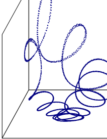
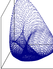
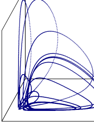
Figure 2: 3D projections on the $x_{2},x_{3},x_{4}$ plane for the system with $(k_{1},k_{2},k_{3},k_{4})=(-1,-4,-2,-1)$ and for initial conditions: (a) close to a fixed point of Fig.1(d) ($E=6$), (b) on an ellipse around the fixed point ($E=6$), (c) randomly chosen from Fig.1(d) ($E=6$) and (d) randomly chosen at a higher total energy ($E=20$) exhibiting chaotic behavior.

with different $k_{1},\ldots,k_{4}$ values, which are complementary to the two integrable cases described by Theorem 5.2. We numerically integrate the system’s equations of motion together with its variational equations to compute the value of the largest Lyapunov exponent $\lambda$. The variational equations of the system (14) are

$$\delta\dot{\mathbf{x}}=[J\cdot\nabla^{2}H(\mathbf{x}(t))]\cdot\delta\mathbf{x}~{}~{},$$ (15)

where $\delta\mathbf{x}=(\delta x_{1},\delta x_{2},\delta x_{3},\delta x_{4})$ is a vector which evolves on the tangent space of the system (14) and $\nabla^{2}H$ denotes the Hessian matrix of the Hamiltonian function $H$ calculated along the reference orbit $\mathbf{x}(t)$ of the system (14). In particular, we used the classical Runge–Kutta forth-order scheme with time-step $\tau=10^{-4}$ for the numerical integration of the systems (14) and (15), which conserved the energy $E=H(\mathbf{x})$ of the system (14) with accuracy of more than 8 significant figures during integration times of the order of a few thousand. The indicator which controls of the relative energy error is

$$RE=\log_{10}\left|\frac{E(t)-E_{0}}{E_{0}}\right|~{}~{},$$

where $E_{0}$ is the initial energy of the system and $E(t)$ the actual energy during the numerical integration.

For $k_{i}<0$, $i=1,\dots 4$, the point $\mathbf{x}_{0}=(-k_{1},-k_{2},-k_{3},-k_{4})$ is an elliptic fixed point of the system. Furthermore, in this case $H(\mathbf{x})$ admits a global minimum at $\mathbf{x}_{0}$ and all the orbits of the system are bounded.

We start our numerical study with examples of bounded motion, which correspond to negative values for all $k_{i}$. In Fig.1 some Poincaré surfaces of section $x_{2}=1$, $x_{1}>1$ are shown for different $k_{i}<0$ values at $E=6$. However, at this energy level all of them exhibit regular behavior. These Poincaré surfaces of section are constructed for a grid of initial conditions on the $x_{3},x_{4}$ plane, with $x_{2}=1$ and $x_{1}$ found numerically by Newton’s method requiring that $H(\mathbf{x})=E$. We find a rich morphology consisting of periodic and quasiperiodic trajectories, island chains as well as separatrices. Each fixed point on the Poincaré surface represents a periodic orbit, while the ellipse-like curves correspond to quasiperiodic trajectories lying on tori. Fig.2 presents different trajectories projected on the $x_{2},x_{3},x_{4}$ plane for the system with $(k_{1},k_{2},k_{3},k_{4})=(-1,-4,-2,-1)$ which corresponds to Fig.1(d). The first three panels of Fig.2 correspond to $E=6$ and the last one to $E=20$.

Figure 3: The Poincaré surface of section $x_{2}=1,x_{1}>1$ for the Lotka–Volterra system with $a_{i}=1$ and $k_{i}=-1$, $i=1,2,3,4$ for the energies: (a) $E=4.2$, (b) $E=6$, (c) $E=8$, (d) $E=29$.

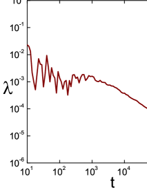
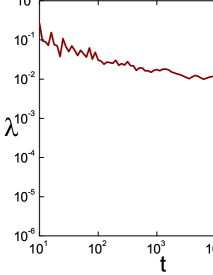
Figure 4: The largest Lyapunov exponent $\lambda$ for the Lotka–Volterra system with $a_{i}=1$ and $k_{i}=-1$, $i=1,2,3,4$ for the energies: (a) $E=4.2$ and (b) $E=29$.

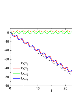
Figure 5: The evolution in time of the phase space variables for the integrable cases: (a) $(k_{1},k_{2},k_{3},k_{4})=(0,0,-1,-1)$ and (b) $(k_{1},k_{2},k_{3},k_{4})=(-2,-2,-2,2)$.

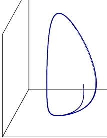
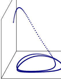
Figure 6: The trajectories projected on the 3D plane $x_{1},x_{3},x_{4}$ plane for the integrable systems: (a) $(k_{1},k_{2},k_{3},k_{4})=(0,0,-1,-1)$ and (b) $(k_{1},k_{2},k_{3},k_{4})=(-2,-2,-2,2)$.

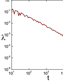
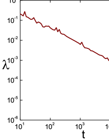
Figure 7: The largest Lyapunov exponent $\lambda$ for the system with $(k_{1},k_{2},k_{3},k_{4})=(-2,-2,-2,2)$ at (b) $E=10$ and (c) $E=72$.

We find qualitatively similar behavior to the examples of Fig.1 for $k_{1}=\dots=k_{4}=-1$, as Fig.3 indicates. In the Poincaré surface of section $x_{2}=1$, $x_{1}>1$ of Fig.3(a), which corresponds to the energy $E=4.2$, there is no evidence of chaotic behavior. We verify this result in Fig.4(a) by computing the largest Lyapunov exponent $\lambda$, which approximately decays as $1/t$ for randomly chosen initial conditions. Similarly with the well-known Hénon–Heiles model [9], chaotic dynamics in the Lotka–Volterra system (14) for $k_{i}<0$ (or $k_{i}=-1$) emerges for larger values of the energy. In the rest of the panels of Fig.3, where the total energy $E$ is gradually increased, we observe a gradual transformation of fixed points and ellipses–like curves, while at energies of the order of $E=30$ (Fig.3(d)) the chaotic motion is not only evident but also prevails over the ordered motion. The largest Lyapunov exponent at this energy, which is plotted in Fig.4(b), converges to a positive value $\lambda\simeq 0.01$.

As we have seen in example 5.3, the only integrable cases for $n=4$, ${\mathbf{a}}=(1,1,1,1)$ predicted by Theorem 5.2 are for $\mathbf{k}=(0,0,k_{3},k_{4})$, $k_{3},k_{4}\in\mathbb{R}$ or $\mathbf{k}=(k_{1},k_{2},0,0)$, $k_{1},k_{2}\in\mathbb{R}$. We choose $(k_{1},k_{2},k_{3},k_{4})=(0,0,-1,-1)$, for which the quantity $(x_{1}+x_{2})x_{4}/x_{3}$ is preserved besides the Hamiltonian. Fig.5(a) displays the evolution of the four variables $\log x_{i}$ in time for a random choice of initial conditions. It turns out that $x_{2}$ decays asymptotically to zero, approximately like $e^{-0.63t}$, while the rest variables $x_{1},x_{3},x_{4}$ asymptotically approach a periodic orbit, as is illustrated in Fig.6(a). However, a similar behavior appears in other cases, not described as integrable by Theorem 5.2. Such an example is given in Fig.5(b) and corresponds to $(k_{1},k_{2},k_{3},k_{4})=(-2,-2,-2,2)$. It turns our that the variables $x_{2}$ and $x_{4}$ tend asymptotically to zero as $e^{-2t}$, while $x_{1}$ and $x_{3}$ asymptotically converge to the periodic orbit shown in Fig.6(b). Furthermore, we carefully examine the largest Lyapunov exponent $\lambda$ in Fig.7 for constantly increasing energies and we find that $\lambda\propto 1/t$, even when $E=72$, which strongly indicates that the system is integrable in this case too.

Similarly to the case $(k_{1},k_{2},k_{3},k_{4})=(-2,-2,-2,2)$ we find other cases which display integrable behavior, manifested by asymptotically vanishing Lyapunov exponents. Few of the cases that we checked are listed in the following table

$k_{1}$	$k_{2}$	$k_{3}$	$k_{4}$
1	1	-1	-1
1	-1	1	-1
1	-1	-1	1
-1	-1	1	-1
-1	1	-1	-1
1	-1	-1	-1

Finally, based on our numerical findings and observations, we conjecture that chaotic motion for the $n=4$ system (7) emerges when $a_{i}>0$, $k_{i}<0$ and $a_{i}<0$, $k_{i}>0$.

7 Conclusions

We presented a new class of Hamiltonian parametric Lotka–Volterra systems with non-zero linear terms and we proved that, for particular choices of parameters, Liouville integrability and superintegrability is established. Different choices of parameters when $n=4$, not described by the theory, were studied numerically, showing that both chaotic and new integrable cases appear. Concerning these new cases with integrable behavior, we aim to study them in detail in order to detect additional integrals and complete our investigation by including all the odd dimensional cases too.

In the present work we restricted our analysis to the even-dimensional case; however, a similar approach can be considered for odd dimensions. Finally, we believe that a similar approach can be considered for integrable Lotka–Volterra systems with different community matrices, or integrable deformations of them such as the systems presented in [6, 7, 8], by inserting parametric linear terms in the corresponding vector fields.

Appendix A Comments and examples on the odd dimensional cases

As it is stated in Section 3, in the odd dimensional cases the described Hamiltonian formalism, i.e. the log-canonical Poisson structure (6) along with the Hamiltonian $H(\mathbf{x})=\sum_{i=1}^{n}(a_{i}x_{i}+k_{i}\log x_{i}),$ is not sufficient to include all the cases of vector fields (1) for arbitrary $r_{i}$, since matrix (5) is not invertible. Therefore, in this setting we can only restrict to the cases with $\mathbf{r}=P\mathbf{k}$, that is systems of the form (7). For $n=3$, the integrability of (7) follows directly from its Hamiltonian formalism and the existence of the Casimir function $\frac{x_{1}x_{3}}{x_{2}}$. More interesting integrable cases emerge for odd $n>3$, by considering the corresponding integrals of the $\mathbf{k}=0$ case as they appear in [14] and the corresponding permutation symmetry of the system. We will illustrate this in the following example for $n=5$.

Let us consider the system

$$\dot{x_{i}}=x_{i}\left(\sum_{j=1}^{5}P_{ij}(a_{j}x_{j}+k_{j})\right)\;,\ \ i=1,\dots,5,$$ (16)

with parameters $\mathbf{a}=(a_{1},\dots,a_{5}),\mathbf{k}=(k_{1},\dots,k_{5})\in\mathbb{R}^{5}$. According to [14], for $\mathbf{k=0}$ this system admits the first integral

$$F=\frac{x_{5}}{x_{4}}(a_{1}x_{1}+a_{2}x_{2}+a_{3}x_{3}).$$

We compute its Poisson bracket with the Hamiltonian $H=\sum_{i=1}^{n}(a_{i}x_{i}+k_{i}\log x_{i})$ of (16) to get

$$\{F,H\}=\frac{x_{5}}{x_{4}}\left(a_{1}(k_{2}+k_{3})x_{1}+a_{2}(k_{3}-k_{1})x_{2}-a_{3}(k_{1}+k_{2})\right).$$

Hence, $F$ is a first integral of (16) if and only if

$$a_{1}(k_{2}+k_{3})=a_{2}(k_{3}-k_{1})=a_{3}(k_{1}+k_{2})=0.$$ (17)

If the parameters $\mathbf{a},\mathbf{k}$ satisfy (17), then the integral $F$ in addition to the Casimir function $C=\frac{x_{1}x_{3}x_{5}}{x_{2}x_{4}}$ ensures the complete integrability of the system. Furthermore, the invariance of (16) under the transformation $x_{i}\mapsto x_{6-i}$, $a_{i}\mapsto-a_{6-i}$, $k_{i}\mapsto-k_{6-i}$, implies that

$$\tilde{F}=\frac{x_{1}}{x_{2}}(a_{5}x_{5}+a_{4}x_{4}+a_{3}x_{3}).$$

is a first integral of (16) if and only if

$$a_{5}(k_{4}+k_{3})=a_{4}(k_{3}-k_{5})=a_{3}(k_{5}+k_{4})=0.$$ (18)

So we conclude that system (16) is integrable if the parameters $\mathbf{a},\mathbf{k}$ satisfy (17) or (18).

For example, in the case of $\mathbf{a}\neq 0$, system (16) is integrable if $k_{3}=-k_{2}=k_{1}$ or $k_{3}=-k_{4}=k_{5}$, while the case of $k_{5}=-k_{4}=k_{3}=-k_{2}=k_{1}$ which leads to superintegrability is equivalent to the $\mathbf{k}=0$ case.

References

[1] Á. Ballesteros, A. Blasco and F. Musso, Integrable deformations of Lotka–Volterra systems,
Phys. Lett. A, 375(38) (2011), 3370–3374.
[2] O. I. Bogoyavlenskij, Some constructions of integrable dynamical systems,
Izv. Akad. Nauk SSSR Ser. Mat., 51(4) (1987), 737–766.
[3] O. I. Bogoyavlenskij, Integrable Lotka-Volterra systems,
Regul. Chaotic Dyn., 13(6) (2008), 543–556.
[4] T. Bountis and P. Vanhaecke, Lotka–Volterra systems satisfying a strong Painlevé property,
Phys. Lett. A., 380(47) (2016), 3977–3982.
[5] S. A. Charalambides, P. A. Damianou, and C. A. Evripidou, On generalized Volterra systems,
J. Geom. Phys., 87 (2015), 86–105.
[6]
P. A. Damianou, C. A. Evripidou, P. Kassotakis and P. Vanhaecke, Integrable Reductions of the Bogoyavlenskij–Itoh Lotka-Volterra Systems, J. Math. Phys., 58 (2017), 032704.
[7] C. A. Evripidou, P. Kassotakis and P. Vanhaecke,
Integrable deformations of the Bogoyavlenskij–Itoh Lotka–Volterra systems,
Regul. Chaot. Dyn., 22 (2017), 721–739.
[8] C. A. Evripidou, P. Kassotakis and P. Vanhaecke,
Integrable reductions of the dressing chain, arXiv:1903.02876.
[9] M. Hénon and C. Heiles,
The applicability of the third integral of motion: Some numerical experiments,
Astron. J., 69(1) (1964), 73–79.
[10] B. Hernández–Bermejo and V. Fairén,
Hamiltonian structure and Darboux theorem for families of generalized Lotka–Volterra systems,
J. Math. Phys., 39(11) (1998), 6162–6174.
[11] Y. Itoh, Integrals of a Lotka–Volterra system of odd number of variables,
Progr. Theoret. Phys., 78(3) (1987), 507–510.
[12] Y. Itoh, A combinatorial method for the vanishing of the Poisson brackets of an integrable
Lotka–Volterra system,
J. Phys. A42(2) (2009), 025201.
[13]
P. H. van der Kamp, T. E. Kouloukas, G. R. W. Quispel, D. T. Tran and P. Vanhaecke,
Integrable and superintegrable systems associated with multi-sums of products,
Proc. R. Soc. Lond. Ser. A Math. Phys. Eng. Sci.,
470 (2014), 20140481.
[14]
T. E. Kouloukas, G. R. W. Quispel and P. Vanhaecke,
Liouville integrability and superintegrability of a generalized Lotka–Volterra system and its Kahan discretization,
J. Phys. A: Math. Theor.49 (2016), 225201.
[15] A. J. Lotka. Analytical theory of biological populations.
The Plenum Series on Demographic Methods and Population Analysis.
Plenum Press, New York, 1998. Translated from the 1939 French edition and with an
introduction by David P. Smith and Hélène Rossert.
[16] O. Ragnisco and M. Scalia, The Volterra Integrable case, arXiv:1903.03595.
[17]
Y. B. Suris and O. Ragnisco,
What is the relativistic Volterra lattice?,
Comm. Math. Phys., 200(2) (1999), 445–485.
[18] J. A. Vano, J. C. Wildenberg, M. B. Anderson, J. K. Noel and J. C. Sprott,
Chaos in low-dimensional Lotka–Volterra models of competition,
Nonlinearity19 (2006), 2391–2404.
[19] A. P. Veselov and A. V. Penskoï,
On algebro–geometric Poisson brackets for the Volterra lattice,
Regul. Chaotic Dyn.3(2) (1998), 3–9.
[20] V. Volterra,
Leçons sur la théorie mathématique de la lutte pour la vie.Les Grands Classiques Gauthier–Villars,
Paris, 1931. Reprint 1990.