Doubly Aligned Incomplete Multi-view Clustering

Abstract

Nowadays, multi-view clustering has attracted more and more attention. To date, almost all the previous studies assume that views are complete. However, in reality, it is often the case that each view may contain some missing instances. Such incompleteness makes it impossible to directly use traditional multi-view clustering methods. In this paper, we propose a Doubly Aligned Incomplete Multi-view Clustering algorithm (DAIMC) based on weighted semi-nonnegative matrix factorization (semi-NMF). Specifically, on the one hand, DAIMC utilizes the given instance alignment information to learn a common latent feature matrix for all the views. On the other hand, DAIMC establishes a consensus basis matrix with the help of $L_{2,1}$-Norm regularized regression for reducing the influence of missing instances. Consequently, compared with existing methods, besides inheriting the strength of semi-NMF with ability to handle negative entries, DAIMC has two unique advantages: 1) solving the incomplete view problem by introducing a respective weight matrix for each view, making it able to easily adapt to the case with more than two views; 2) reducing the influence of view incompleteness on clustering by enforcing the basis matrices of individual views being aligned with the help of regression. Experiments on four real-world datasets demonstrate its advantages.

1 Introduction

Many datasets in real world naturally appear in multiple views or come from multiple sources Blum and Mitchell (1998); Schechter et al. (2017), which are called multi-view data. For example, a document can be translated into different languages, and images can be described by different features such as Fourier shape descriptors and K-L expansion coefficients. In multi-view data, these different views often share some consistency and complementary information Sun (2013); Zhao et al. (2017). Such information can be beneficial to learning tasks such as classification and clustering. This leads to a surge of interest in multi-view learning Potthast et al. (2018); Jing et al. (2017), whose goal is to integrate information and give a compatible solution across all views. Nowadays, multi-view learning has been widely studied in different areas such as face recognition, image processing and natural language processing Romero et al. (2017); Xing et al. (2017); Nie et al. (2018).

In all the tasks of multi-view learning, multi-view clustering Bickel and Scheffer (2004); Fan et al. (2017); Nie et al. (2017); Chao et al. (2017) has attracted more and more attentions due to exempting the expensive requirement of data labeling. The goal of multi-view clustering is making full use of multi-view data to get a better clustering result than just simply concatenated views. To date, many multi-view clustering methods have been proposed. Among these methods, one of the most widely used techniques is nonnegative matrix factorization (NMF) Wang et al. (2016b); Li (2016). Lee and Seung (1999) proposes the NMF, which has received much attention because of its straightforward interpretability for applications. Then, some researchers utilize the NMF for multi-view learning, especially multi-view clustering. A joint NMF process with the consistency constraint is formulated in Liu et al. (2013), which performs NMF for each view and pushes each view’s low dimensional representation towards a common consensus. Besides, some researchers have integrated manifold learning and multi-view learning by imposing the manifold regularization on the objective function of NMF respectively for individual views data Wang et al. (2016a); Zong et al. (2017).

Most of the previous studies on multi-view clustering make a common assumption that all of the views are complete. However, in real world applications, multi-view data tend to be incomplete. For example, in the camera network, for some reasons, the camera may temporarily fail, or be blocked by some objects, making the instance missing. Another example is in document clustering, different languages of the documents represent multiple views. However, we may not get all the documents translated into each language. All the above-mentioned cases lead to the incompleteness of multi-view data. As a result, the lack of the whole row or column makes the traditional instance imputation methods fail. So how to make full use of the complementary knowledge hidden in different views and reduce the impact of missing instances are the most challenging problems of incomplete multi-view learning. Recently, some incomplete multi-view clustering methods have been proposed, for example, Li et al. (2014) proposes PVC by utilizing the information of instance alignment to learn a common latent subspace for aligned instances and a private latent representation for unaligned instances via NMF. Borrowing this idea, Zhao et al. (2016) proposes IMG by integrating PVC and manifold learning to learn the global structure over the entire data instances across all views. However, PVC and IMG can only deal with the two-view incomplete multi-view clustering, limiting their application scope. A method for clustering more than two incomplete views is proposed in Shao et al. (2015)(MIC) by filling the missing instances with the average feature values in each incomplete view, then handling the problem with the help of weighted NMF and $L_{2,1}$-Norm regularization Kong et al. (2011); Wu et al. (2018). However, such a simple imputation will cause a great deviation when the missing ratio is large. As a result, incomplete multi-view clustering still faces significant challenges.

In this paper, we propose the Doubly Aligned Incomplete Multi-view Clustering (DAIMC) to meet the challenges. By integrating semi-NMF Ding et al. (2010) and L_2,1-Norm regularized regression model, DAIMC tries to learn a common latent feature matrix for all the views from two aspects of instances aligned and the basis matrix aligned.

Compared with the existing methods around the incomplete multi-view clustering, besides inheriting the strength of semi-NMF with ability to handle negative entries, DAIMC mainly has the following advantages:
1. DAIMC extends PVC. Borrowing the idea of the weighted NMF, DAIMC introduces a respective weight matrix for each incomplete view to assign the missing instances zero weights and the presented instances one weights in each view, making it able to be easily and straightforwardly extended to the scenario with more than two incomplete views.
2. Besides the instance alignment, DAIMC considers the global information by enforcing the basis matrices of individual views being aligned with the help of the L_2,1-Norm regularized regression model, which further reduces the influence of missing instances on clustering performance.
3. An iterative optimization algorithm for DAIMC with convergent guarantee is proposed. Experimental results on four real-world datasets demonstrate its advantages.

The rest of this paper is organized as follows. In Section 2, we overview some related work on semi-NMF and incomplete multi-view clustering. Section 3 proposes our DAIMC and an efficient iterative algorithm of solving it in detail, respectively. Extensive experimental results and analysis are reported in Section 4. Section 5 concludes this paper with future research directions.

2 Related Work

2.1 Semi-nonnegative Matrix Factorization

The semi-NMF Ding et al. (2010) is an effective latent factor learning method , which is the extension of NMF. Given an input data matrix $\textbf{X}\in\mathbb{R}^{M\times N}$, each column of X is an instance vector. The semi-NMF aims to find a matrix $\textbf{U}\in\mathbb{R}^{M\times K}$ and a nonnegative matrix $\textbf{V}\in\mathbb{R}^{N\times K}$ whose product can well approximate the original matrix X. To facilitate discussion, we call U the $basis\ matrix$ and V the $latent\ feature\ matrix$. Thus we can get the following minimization problem

$$\textrm{min}\ \|\textbf{X}-\textbf{U}\textbf{V}^{T}\|_{\emph{\scriptsize{F}}}^{2}$$ (1)

$$\textrm{s.t.}\ \ \textbf{V}\geq 0$$

Similar to NMF, the objective function in (1) is biconvex. Therefore, it is unrealistic to expect an algorithm to find the global minimum. Ding et al. (2010) proposes an iterative updating algorithm to find the locally optimal solution as follows:
Update U (while fixing V) using the rule

$$\textbf{U}=\textbf{X}\textbf{V}(\textbf{V}^{T}\textbf{V})^{-1}$$ (2)

Update V (while fixing U) using

$$\textbf{V}_{jk}\leftarrow\textbf{V}_{jk}\sqrt{\frac{(\textbf{X}^{T}\textbf{U})_{jk}^{+}+[\textbf{V}(\textbf{U}^{T}\textbf{U})^{-}]_{jk}}{(\textbf{X}^{T}\textbf{U})_{jk}^{-}+[\textbf{V}(\textbf{U}^{T}\textbf{U})^{+}]_{jk}}}$$ (3)

where we separate the positive and negative parts of a matrix A as:

$$\textbf{A}_{jk}^{+}=(|\textbf{A}_{jk}|+\textbf{A}_{jk})/2,\qquad\textbf{A}_{jk}^{-}=(|\textbf{A}_{jk}|-\textbf{A}_{jk})/2.$$ (4)

2.2 Incomplete Multi-view Clustering

Given a dataset with $N$ instances, $C$ categories, $n_{v}$ views $\{\textbf{X}^{(i)},i=1,2,...,n_{v}\}$, where $\textbf{X}^{(v)}\in\mathbb{R}^{d_{v}\times N}$ is the $v$-th view of the dataset. An indicator matrix $\textbf{M}\in\mathbb{R}^{n_{v}\times N}$ for incomplete multi-view clustering problem is defined as:

$$\textbf{M}_{ij}=\begin{cases}1&\text{if $j$-th instance is in the $i$-th view}\\ 0&\text{otherwise}\end{cases}$$ (5)

where each row of M is the instance presence for corresponding view. If every view contains all the instances, then the matrix M is an all one matrix. And if the $v$-th view is incomplete, the data matrix $\textbf{X}^{(v)}$ will have a number of column missing, $i.e.,\sum_{j=1}^{N}\textbf{M}_{vj}<N.$

The aim of the incomplete multi-view clustering is to integrate all the incomplete views to cluster the $N$ instances into $C$ clusters.

3 Proposed Approach

In this section, we present our Doubly Aligned Incomplete Multi-view Clustering(DAIMC) in detail. We model the DAIMC as a joint weighted semi-NMF problem and use $L_{2,1}$-norm regularized regression to enforce the basis matrix of individual views being aligned. In the following, we propose our model in two aspects and then give a unified objective function for implementing DAIMC.

3.1 Weighted Semi-NMF for Incomplete Multi-view Data

For the $v$-th view, similarly to the weighted NMF, the weighted semi-NMF factorizes the data matrix $\textbf{X}^{(v)}\in\mathbb{R}^{d_{v}\times N}$ into two matrix $\textbf{U}^{(v)}$ and $\textbf{V}^{(v)}$, where $\textbf{U}^{(v)}\in\mathbb{R}^{d_{v}\times K}$, $\textbf{V}^{(v)}\in\mathbb{R}^{N\times K}$,while giving different weights to the reconstruction errors of different instances. $K$ denotes dimension of subspace. In the experiments of previous works Shao et al. (2015); Zhao et al. (2016), for multi-view clustering, the $K$ is set to the number of the categories of the data matrix $\textbf{X}^{(v)}$, i.e., $K=C$. As a result, the weighted semi-NMF optimization problem is formulated as:

$$\textrm{min}\ \|(\textbf{X}^{(v)}-\textbf{U}^{(v)}\textbf{V}^{(v)^{T}})\textbf{W}^{(v)}\|_{\emph{\scriptsize{F}}}^{2}$$ (6)

$$\textrm{s.t.}\ \ \textbf{V}^{(v)}\geq 0$$

where the weight matrix $\textbf{W}^{(v)}\in\mathbf{R}^{N\times N}$ is a diagonal matrix.

$$\textbf{W}_{jj}^{(i)}=\begin{cases}1&\text{if $j$-th instance is in the $i$-th view}\\ 0&\text{otherwise}\end{cases}$$ (7)

Note that $\textbf{W}_{jj}^{(v)}$ indicates the weight of the $j$-th instance in view $v$. If the $j$-th instance is missing, then the loss of this instance will be ignored.

However, (6) only independently decomposes different views without considering their consistency information. To address this issue, we assume that different views have distinct basis matrices $\{\textbf{U}^{(i)}\}_{i=1}^{n_{v}}$ , but share the same latent feature space V. As a result, (6) is rewritten as follows:

$$\textrm{min}\ \sum_{i=1}^{n_{v}}\|(\textbf{X}^{(i)}-\textbf{U}^{(i)}\textbf{V}^{T})\textbf{W}^{(i)}\|_{\emph{\scriptsize{F}}}^{2}$$ (8)

$$\textrm{s.t.}\ \ \textbf{V}\geq 0$$

By solving (8), we can obtain a common representation V for multiple incomplete-view instances.

3.2 $L_{2,1}$-Norm Regularized Regression with Basis Matrix

To further reduce the influence of the missing instances, DAIMC attempts to incorporate the global information among views. In multi-view data, different views have different representations for a same data matrix. Thus, we can align the different basis matrices $\{\textbf{U}^{(i)}\}_{i=1}^{n_{v}}$ of individual views with the help of regression by solving the following problem for the basis matrices intended to be aligned.

$$\textrm{min}\ \sum_{i=1}^{n_{v}}\|\textbf{B}^{(i)^{T}}\textbf{U}^{(i)}-\textbf{U}^{(*)}\|_{\emph{\scriptsize{F}}}^{2}+\beta\|\textbf{B}^{(i)}\|_{2,1}$$ (9)

where $\textbf{B}^{(i)}\in\mathbb{R}^{d_{i}\times K}$ is the regression coefficient matrix for view $i$. The $L_{2,1}$-norm regularization term is here introduced for ensuring $\textbf{B}^{(i)}$ sparse in rows. In this way, $\textbf{B}^{(i)}$ performs a feature selection during the alignment process. The matrix $\textbf{U}^{(*)}\in\mathbb{R}^{P\times K}$ is the same low dimensional representation for the basis matrices of all the views. $P$ denotes dimension of subspace. The value of $P$ will affect the result. Instead of looking for an appropriate $P$, we simply set the matrix $\textbf{U}^{(*)}$ equal to a $K$ dimensional identity matrix $\textbf{I}_{K}$, whose columns correspond to the cluster encodings. For such a setting, our experiments later confirm its effectiveness. As a result, (9) is rewritten as:

$$\textrm{min}\ \sum_{i=1}^{n_{v}}\|\textbf{B}^{(i)^{T}}\textbf{U}^{(i)}-\textbf{I}\|_{\emph{\scriptsize{F}}}^{2}+\beta\|\textbf{B}^{(i)}\|_{2,1}$$ (10)

where $\beta$ is the trade-off hyper-parameter between sparsity and accuracy of regression for the $i$-th view, $\|.\|_{2,1}$ is the $L_{2,1}$ norm and defined as:

$$\|\textbf{B}^{(v)}\|_{2,1}=\sum_{i=1}^{d_{v}}\sqrt{\sum_{j=1}^{K}{\textbf{B}^{(v)}_{ij}}^{2}}$$

3.3 Unified Objective Function

Considering the objective for instance alignment information as well as the basis matrix alignment information simultaneously, we minimize the following objective function

$$\mathcal{J}= \sum_{i=1}^{n_{v}}\big{\{}\|(\textbf{X}^{(i)}-\textbf{U}^{(i)}\textbf{V}^{T})\textbf{W}^{(i)}\|_{\emph{\scriptsize{F}}}^{2}$$ (11)

$$+\alpha(\|\textbf{B}^{(i)^{T}}\textbf{U}^{(i)}-\textbf{I}\|_{\emph{\scriptsize{F}}}^{2}+\beta\|\textbf{B}^{(i)}\|_{2,1})\big{\}}$$

s.t. $$\ \textbf{V}\geq 0$$

where $\alpha$ is nonnegative hyper-parameter that controls the trade-off between the aforementioned two objectives.

3.4 Optimization

The objective function in Eq.(11) is not convex over all variables $\{\textbf{U}^{(i)}\}_{i=1}^{n_{v}}$, V, $\{\textbf{B}^{(i)}\}_{i=1}^{n_{v}}$, simultaneously. To solve this optimization problem, we propose an alternating iteration procedure.
Subproblem of $\{\textbf{U}^{(i)}\}_{i=1}^{n_{v}}$. With $\{\textbf{B}^{(i)}\}_{i=1}^{n_{v}}$ and V fixed, for each $\textbf{U}^{(i)}$, we need to minimize the following objective function:

$$\mathcal{J}(\textbf{U}^{(i)})=\|(\textbf{X}^{(i)}-\textbf{U}^{(i)}\textbf{V}^{T})\textbf{W}^{(i)}\|_{\emph{\scriptsize{F}}}^{2}+\alpha\|\textbf{B}^{(i)^{T}}\textbf{U}^{(i)}-\textbf{I}\|_{\emph{\scriptsize{F}}}^{2}$$ (12)

The partial derivation of $\mathcal{J}(\textbf{U}^{(i)})$ with respect to $\textbf{U}^{(i)}$ is

$$\frac{\partial\mathcal{J}}{\partial\textbf{U}^{(i)}}= 2(\textbf{U}^{(i)}\textbf{V}^{T}-\textbf{X}^{(i)})\textbf{W}^{(i)}\textbf{W}^{(i)^{T}}\textbf{V}+$$ (13)

$$2\alpha\textbf{B}^{(i)}(\textbf{B}^{(i)^{T}}\textbf{U}^{(i)}-\textbf{I})$$

From the definition of $\textbf{W}^{(i)}$, we can see $\textbf{W}^{(i)}=\textbf{W}^{(i)}\textbf{W}^{(i)^{T}}$. Let $\partial\mathcal{J}/\partial\textbf{U}^{(i)}=0$, we get the following equation:

$$(\textbf{U}^{(i)}\textbf{V}^{T}-\textbf{X}^{(i)})\textbf{W}^{(i)}\textbf{V}+\alpha\textbf{B}^{(i)}(\textbf{B}^{(i)^{T}}\textbf{U}^{(i)}-\textbf{I})=0$$ (14)

Eq.(14) is called the $continuous\ Sylvester\ equation$ with respect to $\textbf{U}^{(i)}$, which often arises in control theory. When both $d_{i}$ and $K$ are small, we can solve Eq.(14) via vectorization and get the following updating rule for $\textbf{U}^{(i)}$:

$$vec(\textbf{U}^{(i)})= [\textbf{I}_{K}\otimes(\alpha\textbf{B}^{(i)}\textbf{B}^{(i)^{T}})+(\textbf{V}^{T}\textbf{W}^{(i)}\textbf{V})\otimes\textbf{I}_{d_{i}}]^{-1}$$ (15)

$$vec(\textbf{X}^{(i)}\textbf{W}^{(i)}\textbf{V}+\alpha\textbf{B}^{(i)})$$

And when both $d_{i}$ and $K$ are large, we instead solve it via $Conjugate\ Gradient$. In our experiments, we use the $lyap$ function of MATLAB to solve Eq.(14).
Subproblem of V. With $\{\textbf{B}^{(i)}\}_{i=1}^{n_{v}}$ and $\{\textbf{U}^{(i)}\}_{i=1}^{n_{v}}$ fixed, we need to minimize the following objective function:

$$\mathcal{J}(\textbf{V})=\ \sum_{i=1}^{n_{v}}\|(\textbf{X}^{(i)}-\textbf{U}^{(i)}\textbf{V}^{T})\textbf{W}^{(i)}\|_{\emph{\scriptsize{F}}}^{2}$$ (16)

$$\textrm{s.t.}\ \ \textbf{V}\geq 0$$

The partial derivation of $\mathcal{J}(\textbf{V})$ with respect to V is

$$\frac{\partial\mathcal{J}}{\partial\textbf{V}}=\ \sum_{i=1}^{n_{v}}\big{\{}2\textbf{W}^{(i)}\textbf{V}\textbf{U}^{(i)^{T}}\textbf{U}^{(i)}-2\textbf{W}^{(i)}\textbf{X}^{(i)^{T}}\textbf{U}^{(i)}\big{\}}$$ (17)

Similar to the optimization of semi-NMF, using the KKT complementary condition for the nonnegativity of V, we get

$$(\sum_{i=1}^{n_{v}}\textbf{W}^{(i)}\textbf{V}\textbf{U}^{(i)^{T}}\textbf{U}^{(i)}-\sum_{i=1}^{n_{v}}\textbf{W}^{(i)}\textbf{X}^{(i)^{T}}\textbf{U}^{(i)})_{jk}\textbf{V}_{jk}=0$$ (18)

Based on this equation, we can write the updating rule for V as:

$$\textbf{V}_{jk}\leftarrow\textbf{V}_{jk}$$ (19)

$$\sqrt{\frac{\sum_{i=1}^{n_{v}}\big{\{}[\textbf{W}^{(i)}(\textbf{X}^{(i)^{T}}\textbf{U}^{(i)})^{+}]_{jk}+[\textbf{W}^{(i)}\textbf{V}(\textbf{U}^{(i)^{T}}\textbf{U}^{(i)})^{-}]_{jk}\big{\}}}{\sum_{i=1}^{n_{v}}\big{\{}[\textbf{W}^{(i)}(\textbf{X}^{(i)^{T}}\textbf{U}^{(i)})^{-}]_{jk}+[\textbf{W}^{(i)}\textbf{V}(\textbf{U}^{(i)^{T}}\textbf{U}^{(i)})^{+}]_{jk}\big{\}}}}$$

It is worth to note that if $\{\textbf{U}^{(i)}\}_{i=1}^{n_{v}}$ and V are a solution of Eq.(11), then $\{\textbf{U}^{(i)}\textbf{Q}\}_{i=1}^{n_{v}}$ and $\textbf{V}\textbf{Q}^{-1}$ will form another solution for any invertible matrix Q. With these requirements, the normalization imposed on $\{\textbf{U}^{(i)}\}_{i=1}^{n_{v}}$ and V are achieved by

$$\textbf{V}\leftarrow\textbf{V}\textbf{Q}^{-1}$$ (20)

$$\textbf{U}^{(i)}\leftarrow\textbf{U}^{(i)}\textbf{Q}$$

where Q is a diagonal matrix formally defined asWang et al. (2016a):

$$\textbf{Q}=diag(\sum_{i}\textbf{V}_{i1},\sum_{i}\textbf{V}_{i2},...,\sum_{i}\textbf{V}_{iK}).$$ (21)

Subproblem of $\{\textbf{B}^{(i)}\}_{i=1}^{n_{v}}$. With $\{\textbf{U}^{(i)}\}_{i=1}^{n_{v}}$ and V fixed, for each $\textbf{B}^{(i)}$, we need to minimize the following objective function:

$$\mathcal{J}(\textbf{B}^{(i)})=\|\textbf{B}^{(i)^{T}}\textbf{U}^{(i)}-\textbf{I}\|_{\emph{\scriptsize{F}}}^{2}+\beta\|\textbf{B}^{(i)}\|_{2,1}$$ (22)

The partial derivation of $\mathcal{J}(\textbf{B}^{(i)})$ with respect to $\textbf{B}^{(i)}$ is

$$\frac{\partial\mathcal{J}}{\partial\textbf{B}^{(i)}}=2\textbf{U}^{(i)}(\textbf{U}^{(i)^{T}}\textbf{B}^{(i)}-\textbf{I})+\beta\textbf{D}^{(i)}\textbf{B}^{(i)}$$ (23)

Where $\textbf{D}^{(i)}$ is a diagonal matrix with the $j$-th diagonal element given by

$$\textbf{D}^{(i)}_{jj}=\frac{1}{\|\textbf{B}_{j:}^{(i)}\|_{2}}$$ (24)

where $\textbf{B}_{j:}^{(i)}$ is the $j$-th row of matrix $\textbf{B}^{(i)}$. Let $\partial\mathcal{J}/\partial\textbf{B}^{(i)}$ = 0, we get the following updating rule for $\textbf{B}^{(i)}$:

$$\textbf{B}^{(i)}=[\textbf{U}^{(i)}\textbf{U}^{(i)^{T}}+0.5\beta\textbf{D}^{(i)}]^{-1}\textbf{U}^{(i)}$$ (25)

Generally, in real-world dataset, $d_{i}\gg K$, thus $\textbf{U}^{(i)}\textbf{U}^{(i)^{T}}+0.5\beta\textbf{D}^{(i)}$ is close to singular. In order to avoid inaccurate results and reduce the complexity of the algorithm, we use the matrix inverse equation Bishop and Nasrabadi (2007), to reformulate the update rules for $\textbf{B}^{(i)}$:

$$\textbf{B}^{(i)}= \frac{2}{\beta}[\textbf{D}^{(i)^{-1}}-\textbf{D}^{(i)^{-1}}\textbf{U}^{(i)}(\textbf{U}^{(i)^{T}}\textbf{D}^{(i)^{-1}}\textbf{U}^{(i)}+0.5\beta\textbf{I})^{-1}$$ (26)

$$\textbf{U}^{(i)^{T}}\textbf{D}^{(i)^{-1}}]\textbf{U}^{(i)}$$

The entire optimization procedure for DAIMC is summarized in Algorithm 1.

Algorithm 1 Optimization of DAIMC

0:  Data matrices for incomplete views $\textbf{X}^{(1)},...,\textbf{X}^{(n_{v})}$, weight matrices $\textbf{W}^{(1)},...,\textbf{W}^{(n_{v})}$, hyper-parameters $\alpha,\beta$, number of clusters $K$.

1:  Initialize $\textbf{V}\in\mathbb{R}^{N\times K}$, $\textbf{U}^{(i)}\in\mathbb{R}^{d_{i}\times K}$ and $\textbf{B}^{(i)}\in\mathbb{R}^{d_{i}\times K}$ $i=1,...,n_{v}$.

2:  repeat

3:     for $i=1$ to $n_{v}$ do

4:        Update $\textbf{U}^{(i)}$ by Eq.(14) and $lyap$ function.

5:        Update $\textbf{B}^{(i)}$ by Eq.(26).

6:     end for

7:     repeat

8:        Update V by Eq.(19).

9:     until Eq.(16) converges

10:     Normalize $\textbf{U}^{(i)}$s and V by Eq.(20).

11:  until Eq.(11) converges

12:  Apply $K$-means on V to get the clustering results.

13:  Output:  Basis matrices $\textbf{U}^{(1)},...,\textbf{U}^{(n_{v})}$, regression coefficient matrices $\textbf{B}^{(1)},...,\textbf{B}^{(n_{v})}$, the common latent feature matrix V and clustering results.

3.5 Convergence and Complexity

$Convergence\ Analysis$. As shown by Algorithm 1, the optimization of DAIMC can be divided into three subproblems, each of which is convex w.r.t one variable. Thus, by finding the optimal solution for each subproblem alternatively, our algorithm can at least find a locally optimal solution.
$Complexity\ Analysis$. The time complexity of DAIMC is dominated by matrix multiplication and inverse operations. In each iteration, the $lyap$ function costs $\mathcal{O}(d_{i}^{3})$ and the matrix inversion in Eq.(26) costs $\mathcal{O}(K^{3})$. The complexities of multiplication operations in updating $\textbf{U}^{(i)}$, V and $\textbf{B}^{(i)}$ are $\mathcal{O}(d_{i}^{2}K+d_{i}N+KN)$, $\mathcal{O}(M(d_{i}KN+d_{i}K^{2}+K^{2}N))$ and $\mathcal{O}(K^{3}+d_{i}^{2}K)$ respectively, where $M$ is the iteration times of the inner loop. In general, $K\leq d_{i}$ and $N$. Suppose $L$, $d_{max}$ are the iteration times of the outer loop and the largest dimensionality of all the views respectively, thus the time complexity of DAIMC is $\mathcal{O}(n_{v}Ld_{max}^{3}+LMd_{max}KN)$.

4 Experiments and Analysis

Datasets: The experiments are conducted on four real-world multi-view datasets. The important statistics of these datasets are given in the Table 1.

  Dataset $\#$ instances $\#$ views $\#$ clusters Wikipedia 693 2 10 Digit 2000 5 10 3Sources 416 3 6 Flowers 1360 3 17  

Table 1: Statistics of the datasets

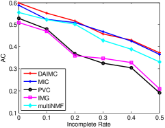
(a) ACs for Wikipedia

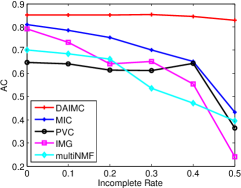
(b) ACs for Digit

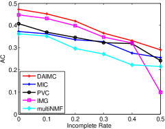
(c) ACs for Flowers

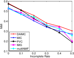
(d) NMIs for Wikipedia

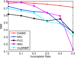
(e) NMIs for Digit

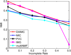
(f) NMIs for Flowers

Figure 1: Performance of clustering on Wikipedia, Digit and Flowers.

Compared methods: In the experiments, DAIMC is compared with the following state-of-the-art multi-view clustering methods. (1)MultiNMF: Multi-view NMF Liu et al. (2013) seeks a common latent subspace based on joint NMF. However, this method can not deal with the incomplete multi-view data, in our experiment, we therefore first fill the missing instances in each incomplete view with average feature values. (2)PVC: Partial multi-view clustering Li et al. (2014) is one of the state-of-art incomplete multi-view clustering methods, which learns a common latent subspace for the aligned instances and a private latent subspace for the unaligned instances. (3)IMG: Incomplete multi-modal visual data grouping Zhao et al. (2016) integrates PVC and manifold learning, which bridges the connection of missing instance data from different views by learning a complete graph Laplacian term. (4)MIC: Multiple incomplete views clustering via weighted NMF Shao et al. (2015) is a feasible method for incomplete multi-view clustering, which first fills the missing instances in each incomplete view with average feature values, then learns a common latent subspace with $L_{2,1}$-norm regularization. All of the hyper-parameters of these methods are selected through grid-search.

For the evaluation metric, we follow Li et al. (2014), using Normalized Mutual Information (NMI). Besides, precision of clustering result is also reported to give a comprehensive view. Similarly to Shao et al. (2015), for the complete datasets, we randomly remove some instances from each view to make the views incomplete. The incomplete rate is from 0 (all the views are complete) to 0.5 (all the views have 50$\%$ instances missing). It is also worth to note that 3Sources is naturally incomplete. Also since PVC and IMG can only deal with two incomplete views, in order to compare PVC and IMG with other methods, we train these models on all the two-views combinations and report the best result.

4.1 Experimental Results

Methods	BBC-Guardian		BBC-Reuters		Guardian-Reuters		3Sources
	NMI	AC	NMI	AC	NMI	AC	NMI	AC
DAIMC	0.4264	0.5399	0.4482	0.5641	0.3805	0.5124	0.4733	0.5963
MIC	0.3813	0.4988	0.3814	0.4912	0.3800	0.4612	0.4512	0.5631
PVC	0.2412	0.4334	0.2931	0.4252	0.2488	0.4145	$\backslash$	$\backslash$
IMG	0.2614	0.4511	0.3612	0.4624	0.3411	0.4384	$\backslash$	$\backslash$
MultiNMF	0.3647	0.4693	0.3687	0.4517	0.3487	0.4281	0.4134	0.4756

Table 2: The NMIs and ACs of different methods on various subsets of 3Sources.

Table 2 and Figure 1 report the AC and NMI values on image and text datasets with different incomplete rates, respectively. From these table and figures, we can get the following results.

From Figure 1(a) and Figure 1(d), we can see that on Wikipedia dataset, DAIMC raises the performance around 8.65$\%$ in NMI with different incomplete rate settings. And in AC, the performance of DAIMC and MIC are close for incomplete rates from 0.2 to 0.5 with the interval of 0.1, the difference between the two methods is just 1$\%$. But when the incomplete rate varies from 0 to 0.1, DAIMC outperforms all the other methods by about 3.53$\%$.

From Figure 1(b) and Figure 1(e), we can see that on Digit dataset, the experimental results of DAIMC are much better than those of other methods. Especially when the incomplete rates are large(0.4 and 0.5), DAIMC raises the performance around 60.78$\%$ in NMI and 64.67$\%$ in AC, respectively. The main reason for this phenomenon is due to that the Digit dataset contains 5 views. DAIMC effectively uses information from different views, reduces the impact of missing samples, and obtains better experimental results.

On Flowers dataset, from Figure 1(c) and Figure 1(f), we can easily see that DAIMC raises the performance around 10.29$\%$ in NMI and 20.37$\%$ in AC, respectively. Besides, IMG performs very well when the incomplete rate is small (0-0.4), the main reason is due to that Flowers dataset contains a terrible view $D\_texturegc$, which plays a negative role in clustering results. Thus, the performances of MIC and multiNMF are bad. In spite of this, DAIMC still performs good with the help of aligning basis matrices.

Table 2 shows the results on the 3Sources dataset, we conduct the experiment on all the two-views combinations and the whole dataset. From Table 2, we can also observe that DAIMC outperforms all the other methods in both NMI and AC.

In summary, when dealing with text data or multi-view data that contains less alignment information, IMG often gets poor result. Meanwhile, although MIC can handle the clustering problem with more than two-views, simply filling the missing instances with the global feature average will lead to a deviation, especially when the incomplete rate is large. By utilizing the information of instance alignment and enforcing the alignment among basis matrices, the proposed DAIMC can get better performances no matter whether it is text dataset or image dataset. Especially when the number of views is large, DAIMC yields more better results.

4.2 Convergence Study

For the convergence study, we conduct an experiment on Digit dataset with the incomplete rate of 0.4 and set the hyper-parameters $\{\alpha,\beta\}$ as $\{1e1,1e\textnormal{-}1\}$ respectively. In Figure 2, we show the convergence curve and the NMI values with respect to the number of iterations. The blue curve shows the value of the objective function and the red dashed line indicates the NMI of our method. As can be seen, the algorithm has converged just after 30 iterations.

4.3 View Number Study

In order to demonstrate that the proposed method DAIMC can effectively exploit the information of multiple views, we conduct an experiment on Digit dataset with different view numbers. Similar to convergence study, we set incomplete rate and hyper-parameters $\{\alpha,\beta\}$ as 0.5 and $\{1e1,1e0\}$ respectively. The results are shown in Figure LABEL:plot:viewnumber. Obviously, with the increase of the available view number, we get much better result.

4.4 Hyper-parameter Study

The proposed DAIMC method contains two hyper-parameters $\{\alpha,\beta\}$. We conduct the hyper-parameter experiments on Digit dataset. We set the incomplete rate as 0.3 and 0.5 respectively, and report the clustering performance of DAIMC by ranging $\alpha$ and $\beta$ within the set of $\{1e\textnormal{-}4,1e\textnormal{-}3,1e\textnormal{-}2,1e\textnormal{-}1,1e0,1e1,1e2,1e3\}$. As shown in Figure 2 and Figure 2, DAIMC obtains a relatively good performance when $\alpha=1e1$ and $\beta=\{1e\textnormal{-}1,1e0,1e1\}$.

5 Conclusion

In this paper, we proposed an effective method to deal with incomplete multi-view clustering problem by considering the instance alignment information and enforcing different basis matrices being aligned simultaneously. The experimental results on four real-world multi-view datasets demonstrate the effectiveness of our method. In the future, large scale data will be considered by introducing online learning and incremental learning strategies into our model.

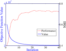
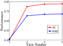
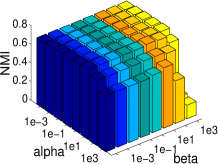
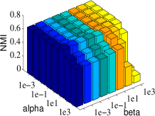
Figure 2: Convergence, view number and hyper-parameter studies on the Digit dataset.

References

- Bickel and Scheffer [2004] Steffen Bickel and Tobias Scheffer. Multi-view clustering. In IEEE International Conference on Data Mining (ICDM), pages 19–26. IEEE Computer Society, 2004.
- Bishop and Nasrabadi [2007] Christopher M Bishop and Nasser M Nasrabadi. Pattern recognition and machine learning. Journal of Electronic Imaging, 16(4):049901, 2007.
- Blum and Mitchell [1998] Avrim Blum and Tom Mitchell. Combining labeled and unlabeled data with co-training. In Annual Conference on Computational Learning Theory (COLT), pages 92–100. ACM, 1998.
- Chao et al. [2017] Guoqing Chao, Shiliang Sun, and Jinbo Bi. A survey on multi-view clustering. arXiv preprint arXiv:1712.06246, 2017.
- Ding et al. [2010] Chris HQ Ding, Tao Li, and Michael I Jordan. Convex and semi-nonnegative matrix factorizations. IEEE Transactions on Pattern Analysis and Machine Intelligence (TPAMI), 32(1):45–55, 2010.
- Fan et al. [2017] Yanbo Fan, Jian Liang, Ran He, Bao-Gang Hu, and Siwei Lyu. Robust localized multi-view subspace clustering. arXiv preprint arXiv:1705.07777, 2017.
- Jing et al. [2017] Xiao-Yuan Jing, Fei Wu, Xiwei Dong, Shiguang Shan, and Songcan Chen. Semi-supervised multi-view correlation feature learning with application to webpage classification. In AAAI Conference on Artificial Intelligence (AAAI), pages 1374–1381, 2017.
- Kong et al. [2011] Deguang Kong, Chris Ding, and Heng Huang. Robust nonnegative matrix factorization using l21-norm. In ACM International Conference on Information and Knowledge Managementn (CIKM), pages 673–682. ACM, 2011.
- Lee and Seung [1999] Daniel D Lee and H Sebastian Seung. Learning the parts of objects by non-negative matrix factorization. Nature, 401(6755):788–791, 1999.
- Li et al. [2014] Shao-Yuan Li, Yuan Jiang, and Zhi-Hua Zhou. Partial multi-view clustering. In AAAI Conference on Artificial Intelligence (AAAI), pages 1968–1974, 2014.
- Li [2016] Yifeng Li. Advances in multi-view matrix factorizations. In International Joint Conference on Neural Networks (IJCNN), pages 3793–3800. IEEE, 2016.
- Liu et al. [2013] Jialu Liu, Chi Wang, Jing Gao, and Jiawei Han. Multi-view clustering via joint nonnegative matrix factorization. In SIAM International Conference on Data Mining (SDM), pages 252–260. SIAM, 2013.
- Nie et al. [2017] Feiping Nie, Guohao Cai, and Xuelong Li. Multi-view clustering and semi-supervised classification with adaptive neighbours. In AAAI Conference on Artificial Intelligence (AAAI), pages 2408–2414, 2017.
- Nie et al. [2018] Feiping Nie, Guohao Cai, Jing Li, and Xuelong Li. Auto-weighted multi-view learning for image clustering and semi-supervised classification. IEEE Transactions on Image Processing, 27(3):1501–1511, 2018.
- Potthast et al. [2018] Christian Potthast, Andreas Breitenmoser, Fei Sha, and Gaurav S Sukhatme. Active multi-view object recognition and online feature selection. In Robotics Research, pages 471–488. Springer, 2018.
- Romero et al. [2017] Andrés Romero, Juan León, and Pablo Arbeláez. Multi-view dynamic facial action unit detection. arXiv preprint arXiv:1704.07863, 2017.
- Schechter et al. [2017] Ian Schechter, Tim Wakeling, and Ann M Wollrath. Processing data from multiple sources, March 28 2017. US Patent 9,607,073.
- Shao et al. [2015] Weixiang Shao, Lifang He, and S Yu Philip. Multiple incomplete views clustering via weighted nonnegative matrix factorization with regularization. In Machine Learning and Knowledge Discovery in Databases - European Conference, ECML PKDD, pages 318–334, 2015.
- Sun [2013] Shiliang Sun. A survey of multi-view machine learning. Neural Computing and Applications, pages 2031–2038, 2013.
- Wang et al. [2016a] Hao Wang, Yan Yang, and Tianrui Li. Multi-view clustering via concept factorization with local manifold regularization. In IEEE International Conference on Data Mining (ICDM), pages 1245–1250, 2016.
- Wang et al. [2016b] Jing Wang, Xiao Wang, Feng Tian, Chang Hong Liu, Hongchuan Yu, and Yanbei Liu. Adaptive multi-view semi-supervised nonnegative matrix factorization. In International Conference on Neural Information Processing (ICONIP), pages 435–444. Springer, 2016.
- Wu et al. [2018] Baolei Wu, Enyuan Wang, Zhen Zhu, Wei Chen, and Pengcheng Xiao. Manifold nmf with norm for clustering. Neurocomputing, 273:78–88, 2018.
- Xing et al. [2017] Junliang Xing, Zhiheng Niu, Junshi Huang, Weiming Hu, Xi Zhou, and Shuicheng Yan. Towards robust and accurate multi-view and partially-occluded face alignment. IEEE Transactions on Pattern Analysis and Machine Intelligence (TPAMI), 2017.
- Zhao et al. [2016] Handong Zhao, Hongfu Liu, and Yun Fu. Incomplete multi-modal visual data grouping. In International Joint Conference on Artificial Intelligence (IJCAI), pages 2392–2398, 2016.
- Zhao et al. [2017] Handong Zhao, Zhengming Ding, and Yun Fu. Multi-view clustering via deep matrix factorization. In AAAI Conference on Artificial Intelligence (AAAI), pages 2921–2927, 2017.
- Zong et al. [2017] Linlin Zong, Xianchao Zhang, Long Zhao, Hong Yu, and Qianli Zhao. Multi-view clustering via multi-manifold regularized non-negative matrix factorization. Neural Networks, 88:74–89, 2017.