Homogenization of Bingham Flow in thin porous media

Abstract

By using dimension reduction and homogenization techniques, we study the steady flow of an incompresible viscoplastic Bingham fluid in a thin porous medium. A main feature of our study is the dependence of the yield stress of the Bingham fluid on the small parameters describing the geometry of the thin porous medium under consideration. Three different problems are obtained in the limit when the small parameter $\varepsilon$ tends to zero, following the ratio between the height $\varepsilon$ of the porous medium and the relative dimension $a_{\varepsilon}$ of its periodically distributed pores. We conclude with the interpretation of these limit problems, which all preserve the nonlinear character of the flow.

María ANGUIANO and Renata BUNOIU

AMS classification numbers: 76A05, 76A20, 76M50, 35B27.

Keywords: porous medium, thin domain, Bingham fluid

1 Introduction

We study in this paper the steady incompressible flow of a Bingham fluid in a thin porous medium containing an array of vertical cylindrical obstacles (the pores). The model of thin porous medium of thickness much smaller than the distance between the pores was introduced in [27], where a stationary incompressible Navier-Stokes flow was studied. Recently, the model of thin porous medium under consideration in this paper was introduced in [15], where the flow of an incompressible viscous fluid described by the stationary Navier-Stokes equations was studied by the multiscale expansion method, which is a formal but powerful tool to analyse homogenization problems. These results were rigorously proved in [4] using an adaptation introduced in [3] of the periodic unfolding method from [12]. This adaptation consists of a combination of the unfolding method with a rescaling in the height variable, in order to work with a domain of fixed height, and to use monotonicity arguments to pass to the limit. In [3], in particular, the flow of an incompressible stationary Stokes system with a nonlinear viscosity, being a power law, was studied. For non-stationary incompressible viscous flow in a thin porous medium see [1], where a non-stationary Stokes system is considered, and [2], where a non-stationary non-newtonian Stokes system, where the viscosity obeyed the power law, is studied. For the periodic unfolding method applied to the study of problems stated in other type of thin periodic domains we refer for instance to [18] for crane type structures and to [19], [20] for thin layers with thin beams structures, where elasticity problems are studied.

If $\Pi$ is a three-dimensional domain with smooth boundary $\partial\Pi$ and $f=(f_{1},f_{2},f_{3})$ are external given forces defined on $\Pi$, then the velocity $u=(u_{1},u_{2},u_{3})$ of a fluid and its pressure $p$ satisfy the equations of motion

$$-\sum_{j=1}^{3}\partial_{x_{i}}(\sigma(p,u))_{ij}=f_{i}\,\,\,\hbox{in}\,\,\Pi,\quad 1\leq i\leq 3,$$ (1)

completed with the fluid’s incompressibility condition ${\textrm{div}}\,u=\sum_{i=1}^{3}\partial_{x_{i}}{u_{i}}=0\hbox{ in }\Pi$, and the no-slip boundary condition $u=0$ on the boundary $\partial\Pi$. What distinguishes different fluids is the expression of the stress tensor $\sigma$. Newtonian fluids are the most encountered ones in real life and as typical examples one can mention the water and the air. For a newtonian fluid, the entries of the stress tensor $\sigma(p,u)$ are given by

$$(\sigma(p,u))_{ij}=-p\delta_{ij}+2\mu(D(u))_{ij},\quad 1\leq i,j\leq 3$$ (2)

where $\delta_{ij}$ is the Kronecker symbol, the real positive $\mu$ is the viscosity of the fluid and the entries of the strain tensor are $(D(u))_{ij}=(\partial_{x_{j}}u_{i}+\partial_{x_{i}}u_{j})/2.$ If $f$ belongs to $(L^{2}(\Pi))^{3}$ and the space $V$ is defined by $\displaystyle V\,\,=\,\,\{v\in(H_{0}^{1}(\Pi))^{3}\,\,|\,\,\mbox{div}\,v=0\},$ then $u$ and $p$ satisfying (1) with (2) are such that (see for instance [17]):

(Stokes) There is a unique $u\in V$ and a unique (up to an additive real constant) $p\in L^{2}(\Pi)$ such that (if $\displaystyle<\cdot,\cdot>$ is the dual pairing between $(H^{-1}(\Pi))^{3}$ and $(H_{0}^{1}(\Pi))^{3}$)

$$a(u,v)=l(v)-<\nabla p,v>,\quad\forall v\in(H_{0}^{1}(\Pi))^{3},$$ (3)

with $\displaystyle a(u,v)=2\mu\int_{\Pi}\hbox{D(u)}\colon\hbox{D(v)}dx$ and $\displaystyle l(v)=\int_{\Pi}f\cdot vdx$.

A fluid whose stress is not defined by relation (2) is called a non-newtonian fluid. There are several classes of non-newtonian fluids, as the power law, Carreau, Cross, Bingham fluids. It is on the study of the last type of fluid that we are interested in this paper. We refer to [13] for a review on non-newtonian fluids. For a Bingham fluid, the nonlinear stress tensor is defined by (see [14])

$$(\sigma(p,u))_{ij}=-p\delta_{ij}+2\mu(D(u))_{ij}+{\sqrt{2}}g\frac{(D(u))_{ij}}{|D(u)|},$$ (4)

where $\displaystyle|D(u)|^{2}=D(u)\colon D(u)$ and the positive number $g$ represents the yield stress of the fluid. If $g=0$, then (4) becomes (2). Viscoplastic Bingham fluids are quite often encountered in real life. As examples one can mention volcanic lava, fresh concrete, the drilling mud, oils, clays and some paintings. For $u_{g}$ and $p_{g}$ satisfying (1) with (4), according to [14], one has the following result:

(Bingham) There is a unique $u_{g}\in V$ and a (non-unique) $p_{g}\in L^{2}(\Pi)/\mathbb{R}$ such that

$$a(u_{g},v-u_{g})+j(v)-j(u_{g})\,\geq\,l(v-u_{g})-<\nabla p_{g},v-u_{g}>,\,\,\forall v\in(H_{0}^{1}(\Pi))^{3}.$$ (5)

Here $\displaystyle a,l,<\cdot,\cdot>$ are as before and

$$j(v)=\sqrt{2}g\int_{\Pi}|D(v)|dx,\quad\forall v\in(H_{0}^{1}(\Pi))^{3}.$$

If the yield stress of the Bingham fluid is of the form $g(\varepsilon)$, with $\varepsilon\in]0,1[$ and such that $g(\varepsilon)$ tends to zero when $\varepsilon$ tends to zero, then, according to [[14], Chapter 6, Théorème 5.1.], the following result holds

When $\varepsilon$ tends to zero, one has for the solution $u_{\varepsilon}$ of problem (5) corresponding to $g(\varepsilon)$ the following convergence

$$u_{\varepsilon}\rightharpoonup u\quad\mbox{ weakly in }V,$$

where $u$ is the solution of problem (3).

This means that, in a fixed domain, the nonlinear character of the Bingham flow is lost in the limit (when the yield stress tends to zero), as it is expected. A natural question that arises is the following: If the yield stress $g(\varepsilon)$ is as before and, moreover, the domain $\Pi$ itself depends on the small parameter $\varepsilon$, what happens when $\varepsilon$ tends to zero? The answer is that, in the limit, the nonlinear character of the flow may be preserved. For instance, if $\Pi_{\varepsilon}$ is a classical rigid porous medium, it was proven in [24] with the asymptotic expansion method that, in a range of parameters, the nonlinear character of the Bingham flow is preserved in the homogenized problem, which is a nonlinear Darcy equation. The convergence corresponding to the above mentioned result was proven in [6] with the two-scale convergence method and then recovered in [8] with the periodic unfolding method. The case of a doubly periodic rigid porous medium was studied in [7], where a more involved nonlinear Darcy equation is derived. Another class of domains for which the nonlinear character of the flow may be preserved in the limit is those of thin domains. The case of a domain $\Pi_{\varepsilon}$ which is thin in one direction was addressed in [10] and [11]. We refer to [9] for the asymptotic analysis of a Bingham fluid in a thin T-like shaped domain. In all these cases, a lower-dimensional Bingham-like law was exhibited in the limit. This law was already encountered in engineering (see [26]), but no rigurous mathematical justification was previously known. For the shallow flow of a viscoplastic fluid we refer the reader to [16], [21], [23] and [22].

In this paper we study the asymptotic behavior of the flow of a viscoplastic Bingham fluid in a thin porous medium. We refer the reader to the very recent paper [5] and the references therein for the application of our study to problems issued from the real life applications. As a first example one can mention the flow of the volcanic lava through dense forests (see [25]). Another important application is the flow of fresh concrete spreading through networks of steel bars.

The paper is organized as follows. In Section 2. we state the problem: we define in (6) the thin porous medium $\Omega_{\varepsilon}$ (see also Figure 1), of height $\varepsilon$ and relative dimension $a_{\varepsilon}$ of its periodically distributed pores. In $\Omega_{\varepsilon}$ we consider the flow of a viscoplastic Bingham fluid with velocity $u_{\varepsilon}$ and pressure $p_{\varepsilon}$ verifying the nonlinear variational inequality (9). In Section 3. we give some a priori estimates for the velocity and for the pressure obtained after the change of variables (10) and verifying (12), and then for the velocity and for the pressure defined in (21). In Section 4. by passing to the limit $\varepsilon\rightarrow 0$, we prove the main convergence results of our paper, stated in Theorems 4.4, 4.6 and 4.8, respectively. Up to our knowledge, problems (4.4), (4.6) and (4.8) are new in the mathematical literature. We conclude in Section 5. with the interpretation of these limit problems, which all three preserve the nonlinear character of the flow; both effects of a nonlinear Darcy equation and a lower dimensional Bingham-like law appear. The paper ends with a list of References.

2 Statement of the problem

A periodic porous medium is defined by a domain $\omega$ and an associated microstructure, or periodic cell $Y^{\prime}=[-1/2,1/2]^{2}$, which is made of two complementary parts: the fluid part $Y^{\prime}_{f}$, and the solid part $Y^{\prime}_{s}$ ($Y^{\prime}_{f}\bigcup Y^{\prime}_{s}=Y^{\prime}$ and $Y^{\prime}_{f}\bigcap Y^{\prime}_{s}=\varnothing$). More precisely, we assume that $\omega$ is a smooth, bounded, connected set in $\mathbb{R}^{2}$, and that $Y_{s}^{\prime}$ is an open connected subset of $Y^{\prime}$ with a smooth boundary $\partial Y_{s}^{\prime}$, such that $\overline{Y}_{s}^{\prime}$ is strictly included in $Y^{\prime}$.

The microscale of a porous medium is a small positive number $a_{\varepsilon}$. The domain $\omega$ is covered by a regular mesh of size $a_{\varepsilon}$: for $k^{\prime}\in\mathbb{Z}^{2}$, each cell $Y^{\prime}_{k^{\prime},a_{\varepsilon}}=a_{\varepsilon}k^{\prime}+a_{\varepsilon}Y^{\prime}$ is divided in a fluid part $Y^{\prime}_{f_{k^{\prime}},a_{\varepsilon}}$ and a solid part $Y^{\prime}_{s_{k^{\prime}},a_{\varepsilon}}$, i.e. is similar to the unit cell $Y^{\prime}$ rescaled to size $a_{\varepsilon}$. We define $Y=Y^{\prime}\times(0,1)\subset\mathbb{R}^{3}$, which is divided in a fluid part $Y_{f}$ and a solid part $Y_{s}$, and consequently $Y_{k^{\prime},a_{\varepsilon}}=Y^{\prime}_{k^{\prime},a_{\varepsilon}}\times(0,1)\subset\mathbb{R}^{3}$, which is also divided in a fluid part $Y_{f_{k^{\prime}},a_{\varepsilon}}$ and a solid part $Y_{s_{k^{\prime}},a_{\varepsilon}}$.

We denote by $\tau(\overline{Y}^{\prime}_{s_{k^{\prime}},a_{\varepsilon}})$ the set of all translated images of $\overline{Y}^{\prime}_{s_{k^{\prime}},a_{\varepsilon}}$. The set $\tau(\overline{Y}^{\prime}_{s_{k^{\prime}},a_{\varepsilon}})$ represents the solids in $\mathbb{R}^{2}$. The fluid part of the bottom $\omega_{\varepsilon}\subset\mathbb{R}^{2}$ of the porous medium is defined by $\omega_{\varepsilon}=\omega\backslash\bigcup_{k^{\prime}\in\mathcal{K}_{\varepsilon}}\overline{Y}^{\prime}_{s_{k^{\prime}},{a_{\varepsilon}}}$, where $\mathcal{K}_{\varepsilon}=\{k^{\prime}\in\mathbb{Z}^{2}:Y^{\prime}_{k^{\prime},{a_{\varepsilon}}}\cap\omega\neq\emptyset\}$. The whole fluid part $\Omega_{\varepsilon}\subset\mathbb{R}^{3}$ in the thin porous medium is defined by

$$\Omega_{\varepsilon}=\{(x_{1},x_{2},x_{3})\in\omega_{\varepsilon}\times\mathbb{R}:0<x_{3}<\varepsilon\}.$$ (6)

We make the assumption that the solids $\displaystyle\tau(\overline{Y}^{\prime}_{s_{k^{\prime}},a_{\varepsilon}})$ do not intersect the boundary $\partial\omega$. We define $Y^{\varepsilon}_{s_{k^{\prime}},a_{\varepsilon}}=Y^{\prime}_{s_{k^{\prime}},a_{\varepsilon}}\times(0,\varepsilon)$. Denote by $S_{\varepsilon}$ the set of the solids contained in $\Omega_{\varepsilon}$. Then, $S_{\varepsilon}$ is a finite union of solids, i.e. $S_{\varepsilon}=\bigcup_{k^{\prime}\in\mathcal{K}_{\varepsilon}}\overline{Y}^{\varepsilon}_{s_{k^{\prime}},a_{\varepsilon}}.$

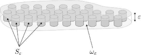
Figure 1: Views of the domain $\Omega_{\varepsilon}$

We define $\widetilde{\Omega}_{\varepsilon}=\omega_{\varepsilon}\times(0,1),$ $\Omega=\omega\times(0,1),$ and $Q_{\varepsilon}=\omega\times(0,\varepsilon).$ We observe that $\widetilde{\Omega}_{\varepsilon}=\Omega\backslash\bigcup_{k^{\prime}\in\mathcal{K}_{\varepsilon}}\overline{Y}_{s_{k^{\prime}},{a_{\varepsilon}}},$ and we define $T_{\varepsilon}=\bigcup_{k^{\prime}\in\mathcal{K}_{\varepsilon}}\overline{Y}_{s_{k^{\prime}},a_{\varepsilon}}$ as the set of the solids contained in $\widetilde{\Omega}_{\varepsilon}$.

We denote by $:$ the full contraction of two matrices; for $A=(a_{i,j})_{1\leq i,j\leq 3}$ and $B=(b_{i,j})_{1\leq i,j\leq 3}$, we have $A:B=\sum_{i,j=1}^{3}a_{ij}b_{ij}$.

In order to apply the unfolding method, we will need the following notation. For $k^{\prime}\in\mathbb{Z}^{2}$, we define $\kappa:\mathbb{R}^{2}\to\mathbb{Z}^{2}$ by

$$\kappa(x^{\prime})=k^{\prime}\iff x^{\prime}\in Y^{\prime}_{k^{\prime},1}\,.$$ (7)

Remark that $\kappa$ is well defined up to a set of zero measure in $\mathbb{R}^{2}$ (the set $\cup_{k^{\prime}\in\mathbb{Z}^{2}}\partial Y^{\prime}_{k^{\prime},1}$). Moreover, for every $a_{\varepsilon}>0$, we have

$$\kappa\left(\frac{x^{\prime}}{a_{\varepsilon}}\right)=k^{\prime}\iff x^{\prime}\in Y^{\prime}_{k^{\prime},a_{\varepsilon}}.$$

We denote by $C$ a generic positive constant which can change from line to line.

The points $x\in\mathbb{R}^{3}$ will be decomposed as $x=(x^{\prime},x_{3})$ with $x^{\prime}=(x_{1},x_{2})\in\mathbb{R}^{2}$, $x_{3}\in\mathbb{R}$. We also use the notation $x^{\prime}$ to denote a generic vector of $\mathbb{R}^{2}$.

In $\Omega_{\varepsilon}$ we consider the stationary flow of an incompressible Bingham fluid. As already seen in the Introduction, following Duvaut and Lions [14], the problem is formulated in terms of a variational inequality.

For a vectorial function $v=(v^{\prime},v_{3})$, we define

$$(D(v))_{i,j}={\frac{1}{2}}\left(\partial_{x_{j}}v_{i}+\partial_{x_{i}}v_{j}\right),\quad 1\leq i,j\leq 3,\quad|D(v)|^{2}=D(v):D(v).$$

We introduce the following spaces

$$V(\Omega_{\varepsilon})=\{v\in(H_{0}^{1}(\Omega_{\varepsilon}))^{3}\,|\,{\rm div}\,v=0\text{ in }\Omega_{\varepsilon}\},\quad H(\Omega_{\varepsilon})=\{v\in(L^{2}(\Omega_{\varepsilon}))^{3}\,|\,{\rm div}\,v=0\text{ in }\Omega_{\varepsilon},v\cdot n=0\text{ on }\partial\Omega_{\varepsilon}\}.$$

For $u,v\in(H_{0}^{1}(\Omega_{\varepsilon}))^{3}$, we introduce

$$a(u,v)=2\mu\int_{\Omega_{\varepsilon}}D(u):D(v)dx,\quad j(v)=\sqrt{2}g(\varepsilon)\int_{\Omega_{\varepsilon}}|D(v)|dx,\quad(u,v)_{\Omega_{\varepsilon}}=\int_{\Omega_{\varepsilon}}u\cdot vdx,$$

where the yield stress $g(\varepsilon)$ will be made precise in Section 3.1. Let $f\in(L^{2}(\Omega))^{3}$ be given such that $f=(f^{\prime},0)$. Let $f_{\varepsilon}\in(L^{2}(\Omega_{\varepsilon}))^{3}$ be defined by

$$f_{\varepsilon}(x)=f(x^{\prime},x_{3}/\varepsilon),\text{\ a.e. \ }x\in\Omega_{\varepsilon}.$$

The model of the flow is described by the following variational inequality:

Find $u_{\varepsilon}\in V(\Omega_{\varepsilon})$ such that

$$a(u_{\varepsilon},v-u_{\varepsilon})+j(v)-j(u_{\varepsilon})\geq(f_{\varepsilon},v-u_{\varepsilon})_{\Omega_{\varepsilon}},\quad\forall v\in V(\Omega_{\varepsilon}).$$ (8)

From Duvaut and Lions [14], we know that there exists a unique $u_{\varepsilon}\in V(\Omega_{\varepsilon})$ solution of problem (8). Moreover, from Bourgeat and Mikelić [6], we know that if $p_{\varepsilon}$ is the pressure of the fluid in $\Omega_{\varepsilon}$, then problem (8) is equivalent to the following one: Find $u_{\varepsilon}\in V(\Omega_{\varepsilon})$ and $p_{\varepsilon}\in L_{0}^{2}(\Omega_{\varepsilon})$ such that

$$a(u_{\varepsilon},v-u_{\varepsilon})+j(v)-j(u_{\varepsilon})\geq(f_{\varepsilon},v-u_{\varepsilon})_{\Omega_{\varepsilon}}+(p_{\varepsilon},{\rm div}\,(v-u_{\varepsilon}))_{\Omega_{\varepsilon}},\quad\forall v\in(H_{0}^{1}(\Omega_{\varepsilon}))^{3}.$$ (9)

Problem (9) admits a unique solution $u_{\varepsilon}\in V(\Omega_{\varepsilon})$ and a (non) unique solution $p_{\varepsilon}\in L_{0}^{2}(\Omega_{\varepsilon})$, where $L_{0}^{2}(\Omega_{\varepsilon})$ denotes the space of functions belonging to $L^{2}(\Omega_{\varepsilon})$ and of mean value zero.

Our aim is to study the asymptotic behavior of $u_{\varepsilon}$ and $p_{\varepsilon}$ when $\varepsilon$ tends to zero. For this purpose, we first use the dilatation of the domain $\Omega_{\varepsilon}$ in the variable $x_{3}$, namely

$$y_{3}=\frac{x_{3}}{\varepsilon},$$ (10)

in order to have the functions defined in an open set with fixed height, denoted $\widetilde{\Omega}_{\varepsilon}$.

Namely, we define $\tilde{u}_{\varepsilon}\in(H_{0}^{1}(\widetilde{\Omega}_{\varepsilon}))^{3}$, $\tilde{p}_{\varepsilon}\in L^{2}_{0}(\widetilde{\Omega}_{\varepsilon})$ by

$$\tilde{u}_{\varepsilon}(x^{\prime},y_{3})=u_{\varepsilon}(x^{\prime},\varepsilon y_{3}),\quad\tilde{p}_{\varepsilon}(x^{\prime},y_{3})=p_{\varepsilon}(x^{\prime},\varepsilon y_{3})\text{\ \ }a.e.\text{\ }(x^{\prime},y_{3})\in\widetilde{\Omega}_{\varepsilon}.$$

Let us introduce some notation which will be useful in the following. For a vectorial function $v=(v^{\prime},v_{3})$ and a scalar function $w$, we will denote $\mathbb{D}_{x^{\prime}}\left[v\right]=\frac{1}{2}(D_{x^{\prime}}v+D_{x^{\prime}}^{t}v)$ and $\partial_{y_{3}}\left[v\right]=\frac{1}{2}(\partial_{y_{3}}v+\partial_{y_{3}}^{t}v)$, where we denote $\partial_{y_{3}}=(0,0,\frac{\partial}{\partial y_{3}})^{t}$. Moreover, associated to the change of variables (10), we introduce the operators: $D_{\varepsilon}$, $\mathbb{D}_{\varepsilon}$, ${\rm div}_{\varepsilon}$ and $\nabla_{\varepsilon}$, defined by

$$(D_{\varepsilon}v)_{i,j}=\partial_{x_{j}}v_{i}\text{\ for \ }i=1,2,3,\ j=1,2,\quad(D_{\varepsilon}v)_{i,3}=\frac{1}{\varepsilon}\partial_{y_{3}}v_{i}\text{\ for \ }i=1,2,3,$$

$$\mathbb{D}_{\varepsilon}\left[v\right]=\frac{1}{2}\left(D_{\varepsilon}v+D^{t}_{\varepsilon}v\right),\quad|\mathbb{D}_{\varepsilon}\left[v\right]|^{2}=\mathbb{D}_{\varepsilon}\left[v\right]:\mathbb{D}_{\varepsilon}\left[v\right],\quad{\rm div}_{\varepsilon}v={\rm div}_{x^{\prime}}v^{\prime}+\frac{1}{\varepsilon}\partial_{y_{3}}v_{3},\quad\nabla_{\varepsilon}w=(\nabla_{x^{\prime}}w,\frac{1}{\varepsilon}\partial_{y_{3}}w)^{t}.$$

We introduce the following spaces

$$V(\widetilde{\Omega}_{\varepsilon})=\{\tilde{v}\in(H_{0}^{1}(\widetilde{\Omega}_{\varepsilon}))^{3}\,|\,{\rm div}_{\varepsilon}\tilde{v}=0\text{ in }\widetilde{\Omega}_{\varepsilon}\},\quad H(\widetilde{\Omega}_{\varepsilon})=\{\tilde{v}\in(L^{2}(\widetilde{\Omega}_{\varepsilon}))^{3}\,|\,{\rm div}_{\varepsilon}\tilde{v}=0\text{ in }\widetilde{\Omega}_{\varepsilon},\tilde{v}\cdot n=0\text{ on }\partial\widetilde{\Omega}_{\varepsilon}\}.$$

For $\tilde{u},\tilde{v}\in V(\widetilde{\Omega}_{\varepsilon})$, we introduce

$$a_{\varepsilon}(\tilde{u},\tilde{v})=2\mu\int_{\widetilde{\Omega}_{\varepsilon}}\mathbb{D}_{\varepsilon}\left[\tilde{u}\right]:\mathbb{D}_{\varepsilon}\left[\tilde{v}\right]dx^{\prime}dy_{3},\quad j_{\varepsilon}(\tilde{v})=\sqrt{2}g(\varepsilon)\int_{\widetilde{\Omega}_{\varepsilon}}|\mathbb{D}_{\varepsilon}[\tilde{v}]|dx^{\prime}dy_{3},\quad(\tilde{u},\tilde{v})_{\widetilde{\Omega}_{\varepsilon}}=\int_{\widetilde{\Omega}_{\varepsilon}}\tilde{u}\cdot\tilde{v}dx^{\prime}dy_{3}.$$

Using the transformation (10), the variational inequality (8) can be rewritten as:

Find $\tilde{u}_{\varepsilon}\in V(\widetilde{\Omega}_{\varepsilon})$ such that

$$a_{\varepsilon}(\tilde{u}_{\varepsilon},\tilde{v}-\tilde{u}_{\varepsilon})+j_{\varepsilon}(\tilde{v})-j_{\varepsilon}(\tilde{u}_{\varepsilon})\geq(f,\tilde{v}-\tilde{u}_{\varepsilon})_{\widetilde{\Omega}_{\varepsilon}},\quad\forall\tilde{v}\in V(\widetilde{\Omega}_{\varepsilon}),$$ (11)

and (9) can be rewritten as:

Find $\tilde{u}_{\varepsilon}\in V(\widetilde{\Omega}_{\varepsilon})$ and $\tilde{p}_{\varepsilon}\in L_{0}^{2}(\widetilde{\Omega}_{\varepsilon})$ such that

$$a_{\varepsilon}(\tilde{u}_{\varepsilon},\tilde{v}-\tilde{u}_{\varepsilon})+j_{\varepsilon}(\tilde{v})-j_{\varepsilon}(\tilde{u}_{\varepsilon})\geq(f,\tilde{v}-\tilde{u}_{\varepsilon})_{\widetilde{\Omega}_{\varepsilon}}+(\tilde{p}_{\varepsilon},{\rm div}_{\varepsilon}(\tilde{v}-\tilde{u}_{\varepsilon}))_{\widetilde{\Omega}_{\varepsilon}},\quad\forall\tilde{v}\in(H_{0}^{1}(\widetilde{\Omega}_{\varepsilon}))^{3}.$$ (12)

Our goal now is to describe the asymptotic behavior of this new sequence $(\tilde{u}_{\varepsilon}$, $\tilde{p}_{\varepsilon})$.

3 A Priori Estimates

We start by obtaining some a priori estimates for $\tilde{u}_{\varepsilon}$.

Lemma 3.1.

There exists a constant $C$ independent of $\varepsilon$, such that if $\tilde{u}_{\varepsilon}\in(H_{0}^{1}(\widetilde{\Omega}_{\varepsilon}))^{3}$ is the solution of problem (11), one has

• if $a_{\varepsilon}\approx\varepsilon$, with $a_{\varepsilon}/\varepsilon\to\lambda$, $0<\lambda<+\infty$, or $a_{\varepsilon}\ll\varepsilon$, then

  $$\left\|\tilde{u}_{\varepsilon}\right\|_{(L^{2}(\widetilde{\Omega}_{\varepsilon}))^{3}}\leq\frac{C}{\mu}a_{\varepsilon}^{2},\quad\left\|\mathbb{D}_{\varepsilon}\left[\tilde{u}_{\varepsilon}\right]\right\|_{(L^{2}(\widetilde{\Omega}_{\varepsilon}))^{{3\times 3}}}\leq\frac{C}{\mu}a_{\varepsilon},\quad\left\|D_{\varepsilon}\tilde{u}_{\varepsilon}\right\|_{(L^{2}(\widetilde{\Omega}_{\varepsilon}))^{{3\times 3}}}\leq\frac{C}{\mu}a_{\varepsilon},$$ (13)

• if $a_{\varepsilon}\gg\varepsilon$, then

  $$\left\|\tilde{u}_{\varepsilon}\right\|_{(L^{2}(\widetilde{\Omega}_{\varepsilon}))^{3}}\leq\frac{C}{\mu}\varepsilon^{2},\quad\left\|\mathbb{D}_{\varepsilon}\left[\tilde{u}_{\varepsilon}\right]\right\|_{(L^{2}(\widetilde{\Omega}_{\varepsilon}))^{{3\times 3}}}\leq\frac{C}{\mu}\varepsilon,\quad\left\|D_{\varepsilon}\tilde{u}_{\varepsilon}\right\|_{(L^{2}(\widetilde{\Omega}_{\varepsilon}))^{{3\times 3}}}\leq\frac{C}{\mu}\varepsilon.$$ (14)

Proof.

Setting successively $\tilde{v}=2\tilde{u}_{\varepsilon}$ and $\tilde{v}=0$ in (11), we have

$$2\mu\int_{\widetilde{\Omega}_{\varepsilon}}\mathbb{D}_{\varepsilon}\left[\tilde{u}_{\varepsilon}\right]:\mathbb{D}_{\varepsilon}\left[\tilde{u}_{\varepsilon}\right]dx^{\prime}dy_{3}+\sqrt{2}g(\varepsilon)\int_{\widetilde{\Omega}_{\varepsilon}}|\mathbb{D}_{\varepsilon}[\tilde{u}_{\varepsilon}]|dx^{\prime}dy_{3}=\int_{\widetilde{\Omega}_{\varepsilon}}f\cdot\tilde{u}_{\varepsilon}\,dx^{\prime}dy_{3}.$$ (15)

Using Cauchy-Schwarz’s inequality and the assumption of $f$, we obtain that

$$\int_{\widetilde{\Omega}_{\varepsilon}}f\cdot\tilde{u}_{\varepsilon}\,dx^{\prime}dy_{3}\leq C\left\|\tilde{u}_{\varepsilon}\right\|_{(L^{2}(\widetilde{\Omega}_{\varepsilon}))^{3}},$$

and taking into account that $\int_{\widetilde{\Omega}_{\varepsilon}}|\mathbb{D}_{\varepsilon}[\tilde{u}_{\varepsilon}]|dx^{\prime}dy_{3}\geq 0,$ by (15), we have

$$\left\|\mathbb{D}_{\varepsilon}\left[\tilde{u}_{\varepsilon}\right]\right\|_{(L^{2}(\widetilde{\Omega}_{\varepsilon}))^{{3\times 3}}}^{2}\leq\frac{C}{\mu}\left\|\tilde{u}_{\varepsilon}\right\|_{(L^{2}(\widetilde{\Omega}_{\varepsilon}))^{3}}.$$

For the cases $a_{\varepsilon}\approx\varepsilon$ or $a_{\varepsilon}\ll\varepsilon$, taking into account Remark 4.3(i) in [3], we obtain the second estimate in (13), and, consequently, from classical Korn’s inequality we obtain the last estimate in (13). Now, from the second estimate in (13) and Remark 4.3(i) in [3], we deduce the first estimate in (13). For the case $a_{\varepsilon}\gg\varepsilon$, proceeding similarly with Remark 4.3(ii) in [3], we obtain the desired result. ∎

3.1 The extension of $(\tilde{u}_{\varepsilon},\tilde{p}_{\varepsilon})$ to the whole domain $\Omega$

We extend the velocity $\tilde{u}_{\varepsilon}$ by zero to the $\Omega\backslash\widetilde{\Omega}_{\varepsilon}$ and denote the extension by the same symbol. Obviously, estimates (13)-(14) remain valid and the extension is divergence free too.

We study in the sequel the following cases for the value of yield stress $g(\varepsilon)$:

• if $a_{\varepsilon}\approx\varepsilon$, with $a_{\varepsilon}/\varepsilon\to\lambda$, $0<\lambda<+\infty$, or $a_{\varepsilon}\ll\varepsilon$, then $\displaystyle g(\varepsilon)=g\,a_{\varepsilon},$

• if $a_{\varepsilon}\gg\varepsilon$, then $\displaystyle g(\varepsilon)=g\,\varepsilon.$

These choices are the most challenging ones and they answer to the question adressed in the paper, namely they all preserve in the limit the nonlinear character of the flow.

In order to extend the pressure to the whole domain $\Omega$, the mapping $R^{\varepsilon}$ (defined in Lemma 4.5 in [3] as $R_{2}^{\varepsilon}$) allows us to extend the pressure $p_{\varepsilon}$ to $Q_{\varepsilon}$ by introducing $F_{\varepsilon}$ in $(H^{-1}(Q_{\varepsilon}))^{3}$:

$$\left\langle F_{\varepsilon},w\right\rangle_{Q_{\varepsilon}}=\left\langle\nabla{p}_{\varepsilon},R^{\varepsilon}w\right\rangle_{{\Omega}_{\varepsilon}},\text{\ for any \ }w\in(H_{0}^{1}(Q_{\varepsilon}))^{3}.$$ (16)

Setting succesively $v=u_{\varepsilon}+R^{\varepsilon}w$ and $v=u_{\varepsilon}-R^{\varepsilon}w$ in (9) we get the inequality

$$|\left\langle F_{\varepsilon},w\right\rangle_{Q_{\varepsilon}}|\leq|a(u_{\varepsilon},R^{\varepsilon}w)|+|(f_{\varepsilon},R^{\varepsilon}w)_{{\Omega}_{\varepsilon}}|+j(R^{\varepsilon}w).$$ (17)

Moreover, if ${\rm div}\,w=0$ then $\left\langle F_{\varepsilon},w\right\rangle_{Q_{\varepsilon}}=0,$ and the DeRham Theorem gives the existence of $P_{\varepsilon}$ in $L_{0}^{2}(Q_{\varepsilon})$ with $F_{\varepsilon}=\nabla P_{\varepsilon}$.

Using the change of variables (10), we get for any $\tilde{w}\in(H_{0}^{1}(\Omega))^{3}$ where $\tilde{w}(x^{\prime},y_{3})=w(x^{\prime},\varepsilon y_{3})$,

$$\left\langle\nabla_{\varepsilon}\tilde{P}_{\varepsilon},\tilde{w}\right\rangle_{\Omega}=-\int_{\Omega}\tilde{P}_{\varepsilon}\,{\rm div}_{\varepsilon}\tilde{w}\,dx^{\prime}dy_{3}=-\varepsilon^{-1}\int_{Q_{\varepsilon}}P_{\varepsilon}\,{\rm div}\,w\,dx=\varepsilon^{-1}\left\langle\nabla P_{\varepsilon},w\right\rangle_{Q_{\varepsilon}}.$$

Then, using the identification (16) of $F_{\varepsilon}$ and the inequality (17),

$$|\left\langle\nabla_{\varepsilon}\tilde{P}_{\varepsilon},\tilde{w}\right\rangle_{\Omega}|\leq\varepsilon^{-1}\left(|a(u_{\varepsilon},R^{\varepsilon}w)|+|(f_{\varepsilon},R^{\varepsilon}w)_{{\Omega}_{\varepsilon}}|+j(R^{\varepsilon}w)\right).$$

and applying the change of variables (10),

$$|\left\langle\nabla_{\varepsilon}\tilde{P}_{\varepsilon},\tilde{w}\right\rangle_{\Omega}|\leq|a_{\varepsilon}(\tilde{u}_{\varepsilon},\tilde{R}^{\varepsilon}\tilde{w})|+|(f,\tilde{R}^{\varepsilon}\tilde{w})_{\widetilde{\Omega}_{\varepsilon}}|+j_{\varepsilon}(\tilde{R}^{\varepsilon}\tilde{w}),$$ (18)

where $\tilde{R}^{\varepsilon}\tilde{w}=R^{\varepsilon}w$ for any $\tilde{w}\in(H_{0}^{1}(\Omega))^{3}$.

Now, we estimate the right-hand side of (18) using the estimates given in Lemma 4.6 in [3].

Lemma 3.2.

There exists a constant $C$ independent of $\varepsilon$, such that the extension $\tilde{P}_{\varepsilon}\in L_{0}^{2}(\Omega)$ of the pressure $\tilde{p}_{\varepsilon}$ satisfies

$$\left\|\tilde{P}_{\varepsilon}\right\|_{L_{0}^{2}(\Omega)}\leq C.$$ (19)

Proof.

Let us estimate $\nabla_{\varepsilon}\tilde{P}_{\varepsilon}$ in the cases $a_{\varepsilon}\approx\varepsilon$ or $a_{\varepsilon}\ll\varepsilon$. We estimate the right-hand side of (18). Using Cauchy-Schwarz’s inequality and from the second estimate in (13) we have

$$|a_{\varepsilon}(\tilde{u}_{\varepsilon},\tilde{R}^{\varepsilon}\tilde{w})| \leq 2\mu\left\|\mathbb{D}_{\varepsilon}\left[\tilde{u}_{\varepsilon}\right]\right\|_{(L^{2}(\widetilde{\Omega}_{\varepsilon}))^{3\times 3}}\left\|D_{\varepsilon}\tilde{R}^{\varepsilon}\tilde{w}\right\|_{(L^{2}(\widetilde{\Omega}_{\varepsilon}))^{3\times 3}}\leq Ca_{\varepsilon}\left\|D_{\varepsilon}\tilde{R}^{\varepsilon}\tilde{w}\right\|_{(L^{2}(\widetilde{\Omega}_{\varepsilon}))^{3\times 3}}.$$

Using the assumption made on the function $f$, we obtain

$$|(f,\tilde{R}^{\varepsilon}\tilde{w})_{\widetilde{\Omega}_{\varepsilon}}|\leq C\left\|\tilde{R}^{\varepsilon}\tilde{w}\right\|_{(L^{2}(\widetilde{\Omega}_{\varepsilon}))^{3}},$$

and by Cauchy-Schwarz’s inequality and taking into account that $|\widetilde{\Omega}_{\varepsilon}|\leq|\Omega|$, we obtain

$$j_{\varepsilon}(\tilde{R}^{\varepsilon}\tilde{w})\leq C\,a_{\varepsilon}\left\|D_{\varepsilon}\tilde{R}^{\varepsilon}\tilde{w}\right\|_{(L^{2}(\widetilde{\Omega}_{\varepsilon}))^{3\times 3}}.$$

Then, from (18), we deduce

$$\left|\left\langle\nabla_{\varepsilon}\tilde{P}_{\varepsilon},\tilde{w}\right\rangle_{\Omega}\right|\leq Ca_{\varepsilon}\left\|D_{\varepsilon}\tilde{R}^{\varepsilon}\tilde{w}\right\|_{(L^{2}(\widetilde{\Omega}_{\varepsilon}))^{3\times 3}}+C\left\|\tilde{R}^{\varepsilon}\tilde{w}\right\|_{(L^{2}(\widetilde{\Omega}_{\varepsilon}))^{3}}.$$

Taking into account the third point in Lemma 4.6 in [3], we have

$$\left|\left\langle\nabla_{\varepsilon}\tilde{P}_{\varepsilon},\tilde{w}\right\rangle_{\Omega}\right| \leq Ca_{\varepsilon}\left(\frac{1}{a_{\varepsilon}}\left\|\tilde{w}\right\|_{(L^{2}(\Omega))^{3}}+\left\|D_{\varepsilon}\tilde{w}\right\|_{(L^{2}(\Omega))^{3\times 3}}\right)+C\left(\left\|\tilde{w}\right\|_{(L^{2}(\Omega))^{3}}+a_{\varepsilon}\left\|D_{\varepsilon}\tilde{w}\right\|_{(L^{2}(\Omega))^{3\times 3}}\right).$$

If $a_{\varepsilon}\approx\varepsilon$ we take into account that $a_{\varepsilon}\ll 1$, and if $a_{\varepsilon}\ll\varepsilon$ we take into account that $a_{\varepsilon}/\varepsilon\ll 1$ and $a_{\varepsilon}\ll 1$, and we see that there exists a positive constant $C$ such that

$$\left|\left\langle\nabla_{\varepsilon}\tilde{P}_{\varepsilon},\tilde{w}\right\rangle_{\Omega}\right| \leq C\left\|\tilde{w}\right\|_{(H_{0}^{1}(\Omega))^{3}},\quad\forall\tilde{w}\in(H_{0}^{1}(\Omega))^{3},$$

and consequently

$$\left\|\nabla_{\varepsilon}\tilde{P}_{\varepsilon}\right\|_{(H^{-1}(\Omega))^{3}}\leq C.$$

It follows that (see for instance Girault and Raviart [17], Chapter I, Corollary 2.1) there exists a representative of $\tilde{P}_{\varepsilon}\in L^{2}_{0}(\Omega)$ such that

$$\left\|\tilde{P}_{\varepsilon}\right\|_{L^{2}_{0}(\Omega)}\leq C\left\|\nabla\tilde{P}_{\varepsilon}\right\|_{(H^{-1}(\Omega))^{3}}\leq C\left\|\nabla_{\varepsilon}\tilde{P}_{\varepsilon}\right\|_{(H^{-1}(\Omega))^{3}}\leq C.$$

Finally, let us estimate $\nabla_{\varepsilon}\tilde{P}_{\varepsilon}$ in the case $a_{\varepsilon}\gg\varepsilon$. Similarly to the previous case, we estimate the right side of (18) by using Cauchy-Schwarz’s inequality and from the second estimate in (14), and we have

$$\left|\left\langle\nabla_{\varepsilon}\tilde{P}_{\varepsilon},\tilde{w}\right\rangle_{\Omega}\right|\leq C\varepsilon\left\|D_{\varepsilon}\tilde{R}^{\varepsilon}\tilde{w}\right\|_{(L^{2}(\widetilde{\Omega}_{\varepsilon}))^{3\times 3}}+C\left\|\tilde{R}^{\varepsilon}\tilde{w}\right\|_{(L^{2}(\widetilde{\Omega}_{\varepsilon}))^{3}}.$$

Taking into account the proof in Lemma 4.5 in [3], the change of variables (10) and that $a_{\varepsilon}\gg\varepsilon$, we can deduce

$$\left|\left\langle\nabla_{\varepsilon}\tilde{P}_{\varepsilon},\tilde{w}\right\rangle_{\Omega}\right| \leq C\varepsilon\left({1\over\varepsilon}\left\|\tilde{w}\right\|_{(L^{2}(\Omega))^{3}}+{1\over\varepsilon}\left\|D_{x^{\prime}}\tilde{w}\right\|_{(L^{2}(\Omega))^{3\times 2}}+{1\over\varepsilon}\left\|\partial_{y_{3}}\tilde{w}\right\|_{(L^{2}(\Omega))^{3}}\right)$$

$$+ C\left(\left\|\tilde{w}\right\|_{(L^{2}(\Omega))^{3}}+a_{\varepsilon}\left\|D_{x^{\prime}}\tilde{w}\right\|_{(L^{2}(\Omega))^{3\times 2}}+\left\|\partial_{y_{3}}\tilde{w}\right\|_{(L^{2}(\Omega))^{3}}\right),$$

and using that $a_{\varepsilon}\ll 1$, we see that there exists a positive constant $C$ such that

$$\left|\left\langle\nabla_{\varepsilon}\tilde{P}_{\varepsilon},\tilde{w}\right\rangle_{\Omega}\right| \leq C\left\|\tilde{w}\right\|_{(H_{0}^{1}(\Omega))^{3}},\quad\forall\tilde{w}\in(H_{0}^{1}(\Omega))^{3},$$

and reasing as the previous case, we have the estimate (19). ∎

According to these extensions, problem (12) can be written as:

$$2\mu\int_{\Omega}\mathbb{D}_{\varepsilon}\left[\tilde{u}_{\varepsilon}\right]:\mathbb{D}_{\varepsilon}\left[\tilde{v}-\tilde{u}_{\varepsilon}\right]dx^{\prime}dy_{3}+\sqrt{2}g(\varepsilon)\int_{\Omega}|\mathbb{D}_{\varepsilon}[\tilde{v}]|dx^{\prime}dy_{3}-\sqrt{2}g(\varepsilon)\int_{\Omega}|\mathbb{D}_{\varepsilon}[\tilde{u}_{\varepsilon}]|dx^{\prime}dy_{3}$$ (20)

$$\geq\int_{\Omega}f\cdot(\tilde{v}-\tilde{u}_{\varepsilon})\,dx^{\prime}dy_{3}+\int_{\Omega}\tilde{P}_{\varepsilon}\,{\rm div}_{\varepsilon}(\tilde{v}-\tilde{u}_{\varepsilon})dx^{\prime}dy_{3},$$

for every $\tilde{v}$ that is the extension by zero to the whole $\Omega$ of a function in $(H_{0}^{1}(\widetilde{\Omega}_{\varepsilon}))^{3}$.

4 Adaptation of the Unfolding Method

The change of variable (10) does not provide the information we need about the behavior of $\tilde{u}_{\varepsilon}$ in the microstructure associated to $\widetilde{\Omega}_{\varepsilon}$. To solve this difficulty, we use an adaptation introduced in [3] of the unfolding method from [12].

Let us recall this adaptation of the unfolding method in which we divide the domain $\Omega$ in cubes of lateral length $a_{\varepsilon}$ and vertical length $1$. For this purpose, given $(\tilde{u}_{\varepsilon},\tilde{P}_{\varepsilon})\in(H_{0}^{1}(\Omega))^{3}\times L^{2}_{0}(\Omega)$, we define $(\hat{u}_{\varepsilon},\hat{P}_{\varepsilon})$ by

$$\hat{u}_{\varepsilon}(x^{\prime},y)=\tilde{u}_{\varepsilon}\left(a_{\varepsilon}\kappa\left(\frac{x^{\prime}}{a_{\varepsilon}}\right)+a_{\varepsilon}y^{\prime},y_{3}\right),\quad\hat{P}_{\varepsilon}(x^{\prime},y)=\tilde{P}_{\varepsilon}\left(a_{\varepsilon}\kappa\left(\frac{x^{\prime}}{a_{\varepsilon}}\right)+a_{\varepsilon}y^{\prime},y_{3}\right),\text{\ \ a.e. \ }(x^{\prime},y)\in\omega\times Y,$$ (21)

where the function $\kappa$ is defined in (7).

Remark 4.1.

For $k^{\prime}\in\mathcal{K}_{\varepsilon}$, the restriction of $(\hat{u}_{\varepsilon},\hat{P}_{\varepsilon})$ to $Y^{\prime}_{k^{\prime},a_{\varepsilon}}\times Y$ does not depend on $x^{\prime}$, whereas as a function of $y$ it is obtained from $(\tilde{u}_{\varepsilon},\tilde{P}_{\varepsilon})$ by using the change of variables $\displaystyle y^{\prime}=\frac{x^{\prime}-a_{\varepsilon}k^{\prime}}{a_{\varepsilon}},$ which transforms $Y_{k^{\prime},a_{\varepsilon}}$ into $Y$.

We are now in position to obtain estimates for the sequences $(\hat{u}_{\varepsilon},\hat{P}_{\varepsilon})$, as in the proof of Lemma 4.9 in [3].

Lemma 4.2.

There exists a constant $C$ independent of $\varepsilon$, such that the couple $(\hat{u}_{\varepsilon},\hat{P}_{\varepsilon})$ defined by (21) satisfies

• if $a_{\varepsilon}\approx\varepsilon$, with $a_{\varepsilon}/\varepsilon\to\lambda$, $0<\lambda<+\infty$, or $a_{\varepsilon}\ll\varepsilon$,

  $$\left\|\hat{u}_{\varepsilon}\right\|_{(L^{2}(\omega\times Y))^{3}}\leq Ca_{\varepsilon}^{2},\quad\left\|\mathbb{D}_{y^{\prime}}\!\left[\hat{u}_{\varepsilon}\right]\right\|_{(L^{2}(\omega\times Y))^{{3\times 2}}}\!\leq\!Ca_{\varepsilon}^{2},\quad\left\|\partial_{y_{3}}\!\left[\hat{u}_{\varepsilon}\right]\right\|_{(L^{2}(\omega\times Y))^{3}}\!\leq\!C\varepsilon\,a_{\varepsilon},$$

• if $a_{\varepsilon}\gg\varepsilon$,

  $$\left\|\hat{u}_{\varepsilon}\right\|_{(L^{2}(\omega\times Y))^{3}}\leq C\varepsilon^{2},\quad\left\|\mathbb{D}_{y^{\prime}}\!\left[\hat{u}_{\varepsilon}\right]\right\|_{(L^{2}(\omega\times Y))^{{3\times 2}}}\!\leq\!Ca_{\varepsilon}\,\varepsilon,\quad\left\|\partial_{y_{3}}\!\left[\hat{u}_{\varepsilon}\right]\right\|_{(L^{2}(\omega\times Y))^{3}}\!\leq\!C\varepsilon^{2},$$

and, moreover, in every cases,

$$\left\|\hat{P}_{\varepsilon}\right\|_{L^{2}_{0}(\omega\times Y)}\leq C.$$

When $\varepsilon$ tends to zero, we obtain for problem (20) different behaviors, depending on the magnitude of $a_{\varepsilon}$ with respect to $\varepsilon$. We will analyze them in the next sections.

4.1 Critical case $a_{\varepsilon}\approx\varepsilon$, with $a_{\varepsilon}/\varepsilon\to\lambda$, $0<\lambda<+\infty$

First, we obtain some compactness results about the behavior of the sequences $(\tilde{u}_{\varepsilon},\tilde{P}_{\varepsilon})$ and $(\hat{u}_{\varepsilon},\hat{P}_{\varepsilon})$ satisfying the a priori estimates given in Lemmas 3.1-i) and 4.2-i), respectively.

Lemma 4.3 (Critical case).

For a subsequence of $\varepsilon$ still denote by $\varepsilon$, there exist $\tilde{u}\in H^{1}(0,1;L^{2}(\omega)^{3})$, where $\tilde{u}_{3}=0$ and $\tilde{u}=0$ on $y_{3}=\{0,1\}$, $\hat{u}\in L^{2}(\omega;H^{1}_{\sharp}(Y)^{3})$ (“$\sharp$” denotes $Y^{\prime}$-periodicity), with $\hat{u}=0$ on $\omega\times Y_{s}$ and $\hat{u}=0$ on $y_{3}=\{0,1\}$ such that $\int_{Y}\hat{u}(x^{\prime},y)dy=\int_{0}^{1}\tilde{u}(x^{\prime},y_{3})dy_{3}$ with $\int_{Y}\hat{u}_{3}dy=0$, and $\hat{P}\in L^{2}_{0}(\omega\times Y)$, independent of $y$, such that

$${\tilde{u}_{\varepsilon}\over a_{\varepsilon}^{2}}\rightharpoonup(\tilde{u}^{\prime},0)\text{\ in \ }H^{1}(0,1;L^{2}(\omega)^{3}),$$ (22)

$${\hat{u}_{\varepsilon}\over a_{\varepsilon}^{2}}\rightharpoonup\hat{u}\text{\ in \ }L^{2}(\omega;H^{1}(Y)^{3}),\quad\hat{P}_{\varepsilon}\rightharpoonup\hat{P}\text{\ in \ }L^{2}_{0}(\omega\times Y),$$ (23)

$${\rm div}_{x^{\prime}}\left(\int_{0}^{1}\tilde{u}^{\prime}(x^{\prime},y_{3})dy_{3}\right)=0\text{\ in \ }\omega,\quad\left(\int_{0}^{1}\tilde{u}^{\prime}(x^{\prime},y_{3})dy_{3}\right)\cdot n=0\text{\ on \ }\partial\omega,$$ (24)

$${\rm div}_{\lambda}\hat{u}=0\text{\ in \ }\omega\times Y,\quad{\rm div}_{x^{\prime}}\left(\int_{Y}\hat{u}^{\prime}(x^{\prime},y)dy\right)=0\text{\ in \ }\omega,\quad\left(\int_{Y}\hat{u}^{\prime}(x^{\prime},y)dy\right)\cdot n=0\text{\ on \ }\partial\omega,$$ (25)

where ${\rm div}_{\lambda}={\rm div}_{y^{\prime}}+\lambda\partial_{y_{3}}$.

Proof.

We refer the reader to Lemmas 5.2, 5.3 and 5.4 in [3] for the proof of (22)-(25). Here, we prove that $\hat{P}$ does not depend on the microscopic variable $y$. To do this, we choose as test function $\tilde{v}(x^{\prime},y)\in\mathcal{D}(\omega;C_{\sharp}^{\infty}(Y)^{3})$ with $\tilde{v}(x^{\prime},y)=0\in\omega\times Y_{s}$ (thus, $\tilde{v}(x^{\prime},x^{\prime}/a_{\varepsilon},y_{3})\in(H_{0}^{1}(\widetilde{\Omega}_{\varepsilon}))^{3}$). Setting $a_{\varepsilon}\tilde{v}(x^{\prime},x^{\prime}/a_{\varepsilon},y_{3})$ in (20) (we recall that $g(\varepsilon)=g\,a_{\varepsilon})$) and using that ${\rm div}_{\varepsilon}\tilde{u}_{\varepsilon}=0$, we have

$$2\mu a_{\varepsilon}\int_{\Omega}\mathbb{D}_{\varepsilon}\left[\tilde{u}_{\varepsilon}\right]:\left(\mathbb{D}_{x^{\prime}}\left[\tilde{v}\right]+\frac{1}{a_{\varepsilon}}\mathbb{D}_{y^{\prime}}\left[\tilde{v}\right]+\frac{1}{\varepsilon}\partial_{y_{3}}\left[\tilde{v}\right]\right)dx^{\prime}dy_{3}-2\mu\int_{\Omega}|\mathbb{D}_{\varepsilon}\left[\tilde{u}_{\varepsilon}\right]|^{2}dx^{\prime}dy_{3}$$ (26)

$$+\sqrt{2}g\,a_{\varepsilon}^{2}\int_{\Omega}\left|\mathbb{D}_{x^{\prime}}\left[\tilde{v}\right]+\frac{1}{a_{\varepsilon}}\mathbb{D}_{y^{\prime}}\left[\tilde{v}\right]+\frac{1}{\varepsilon}\partial_{y_{3}}\left[\tilde{v}\right]\right|dx^{\prime}dy_{3}-\sqrt{2}g\,a_{\varepsilon}\int_{\Omega}|\mathbb{D}_{\varepsilon}[\tilde{u}_{\varepsilon}]|dx^{\prime}dy_{3}$$

$$\geq a_{\varepsilon}\int_{\Omega}f^{\prime}\cdot\tilde{v}^{\prime}\,dx^{\prime}dy_{3}-\int_{\Omega}f^{\prime}\cdot\tilde{u}^{\prime}_{\varepsilon}\,dx^{\prime}dy_{3}+a_{\varepsilon}\int_{\Omega}\tilde{P}_{\varepsilon}\,{\rm div}_{x^{\prime}}\tilde{v}^{\prime}\,dx^{\prime}dy_{3}+\int_{\Omega}\tilde{P}_{\varepsilon}\,{\rm div}_{y^{\prime}}\tilde{v}^{\prime}\,dx^{\prime}dy_{3}+\frac{a_{\varepsilon}}{\varepsilon}\int_{\Omega}\tilde{P}_{\varepsilon}\,\partial_{y_{3}}\tilde{v}_{3}\,dx^{\prime}dy_{3}.$$

By the change of variables given in Remark 4.1 and by Lemma 4.2, we get for the first term in relation (26)

$$\int_{\Omega}\mathbb{D}_{\varepsilon}\left[\tilde{u}_{\varepsilon}\right]:\left(\mathbb{D}_{x^{\prime}}\left[\tilde{v}\right]+\frac{1}{a_{\varepsilon}}\mathbb{D}_{y^{\prime}}\left[\tilde{v}\right]+\frac{1}{\varepsilon}\partial_{y_{3}}\left[\tilde{v}\right]\right)dx^{\prime}dy_{3}$$

$$=\int_{\omega\times Y}\left(\frac{1}{a_{\varepsilon}}\mathbb{D}_{y^{\prime}}\left[\hat{u}_{\varepsilon}\right]+\frac{1}{\varepsilon}\partial_{y_{3}}\left[\hat{u}_{\varepsilon}\right]\right):\left(\frac{1}{a_{\varepsilon}}\mathbb{D}_{y^{\prime}}\left[\tilde{v}\right]+\frac{1}{\varepsilon}\partial_{y_{3}}\left[\tilde{v}\right]\right)dx^{\prime}dy+O_{\varepsilon},$$

and for the second term in relation (26)

$$\int_{\Omega}|\mathbb{D}_{\varepsilon}\left[\tilde{u}_{\varepsilon}\right]|^{2}dx^{\prime}dy_{3}=\int_{\omega\times Y}\left|\frac{1}{a_{\varepsilon}}\mathbb{D}_{y^{\prime}}\left[\hat{u}_{\varepsilon}\right]+\frac{1}{\varepsilon}\partial_{y_{3}}\left[\hat{u}_{\varepsilon}\right]\right|^{2}dx^{\prime}dy=O_{\varepsilon}.$$ (28)

Moreover, applying the change of variables given in Remark 4.1 to the fourth term in relation (26), we have

$$\int_{\Omega}|\mathbb{D}_{\varepsilon}[\tilde{u}_{\varepsilon}]|dx^{\prime}dy_{3}=\int_{\omega\times Y}\left|\frac{1}{a_{\varepsilon}}\mathbb{D}_{y^{\prime}}\left[\hat{u}_{\varepsilon}\right]+\frac{1}{\varepsilon}\partial_{y_{3}}\left[\hat{u}_{\varepsilon}\right]\right|dx^{\prime}dy.$$ (29)

Therefore, applying the change of variables given in Remark 4.1 to relation (26), we obtain

$$2\mu a_{\varepsilon}\int_{\omega\times Y}\left(\frac{1}{a_{\varepsilon}}\mathbb{D}_{y^{\prime}}\left[\hat{u}_{\varepsilon}\right]+\frac{1}{\varepsilon}\partial_{y_{3}}\left[\hat{u}_{\varepsilon}\right]\right):\left(\frac{1}{a_{\varepsilon}}\mathbb{D}_{y^{\prime}}\left[\tilde{v}\right]+\frac{1}{\varepsilon}\partial_{y_{3}}\left[\tilde{v}\right]\right)dx^{\prime}dy$$ (30)

$$+\sqrt{2}g\,a_{\varepsilon}^{2}\int_{\omega\times Y}\left|\mathbb{D}_{x^{\prime}}\left[\tilde{v}\right]+\frac{1}{a_{\varepsilon}}\mathbb{D}_{y^{\prime}}\left[\tilde{v}\right]+\frac{1}{\varepsilon}\partial_{y_{3}}\left[\tilde{v}\right]\right|dx^{\prime}dy-\sqrt{2}g\,a_{\varepsilon}\int_{\omega\times Y}\left|\frac{1}{a_{\varepsilon}}\mathbb{D}_{y^{\prime}}\left[\hat{u}_{\varepsilon}\right]+\frac{1}{\varepsilon}\partial_{y_{3}}\left[\hat{u}_{\varepsilon}\right]\right|dx^{\prime}dy+O_{\varepsilon}$$

$$\geq a_{\varepsilon}\int_{\omega\times Y}f^{\prime}\cdot\tilde{v}^{\prime}\,dx^{\prime}dy-\int_{\omega\times Y}f^{\prime}\cdot\hat{u}_{\varepsilon}^{\prime}\,dx^{\prime}dy+a_{\varepsilon}\int_{\omega\times Y}\hat{P}_{\varepsilon}\,{\rm div}_{x^{\prime}}\tilde{v}^{\prime}\,dx^{\prime}dy+\int_{\omega\times Y}\hat{P}_{\varepsilon}\,{\rm div}_{y^{\prime}}\tilde{v}^{\prime}\,dx^{\prime}dy$$

$$+\frac{a_{\varepsilon}}{\varepsilon}\int_{\omega\times Y}\hat{P}_{\varepsilon}\,\partial_{y_{3}}\tilde{v}_{3}\,dx^{\prime}dy+O_{\varepsilon}.$$

According with (23), the first term in relation (30) can be written by the following way

$$2\mu a_{\varepsilon}\int_{\omega\times Y}\left(\frac{1}{a_{\varepsilon}^{2}}\mathbb{D}_{y^{\prime}}\left[\hat{u}_{\varepsilon}\right]+{a_{\varepsilon}\over\varepsilon}\frac{1}{a_{\varepsilon}^{2}}\partial_{y_{3}}\left[\hat{u}_{\varepsilon}\right]\right):\left(\mathbb{D}_{y^{\prime}}\left[\tilde{v}\right]+\frac{a_{\varepsilon}}{\varepsilon}\partial_{y_{3}}\left[\tilde{v}\right]\right)dx^{\prime}dy\to 0,\text{ as }\varepsilon\to 0.$$ (31)

In order to pass to the limit in the first nonlinear term, we have

$$\sqrt{2}ga_{\varepsilon}\int_{\omega\times Y}\left|a_{\varepsilon}\mathbb{D}_{x^{\prime}}\left[\tilde{v}\right]+\mathbb{D}_{y^{\prime}}\left[\tilde{v}\right]+\frac{a_{\varepsilon}}{\varepsilon}\partial_{y_{3}}\left[\tilde{v}\right]\right|dx^{\prime}dy\to 0,\text{ as }\varepsilon\to 0.$$ (32)

Now, in order to pass the limit in the second nonlinear term, we are taking into account that

$$\sqrt{2}g\,a_{\varepsilon}\int_{\omega\times Y}\left|\frac{1}{a_{\varepsilon}}\mathbb{D}_{y^{\prime}}\left[\hat{u}_{\varepsilon}\right]+\frac{1}{\varepsilon}\partial_{y_{3}}\left[\hat{u}_{\varepsilon}\right]\right|dx^{\prime}dy=\sqrt{2}g\,a_{\varepsilon}^{2}\int_{\omega\times Y}\left|\frac{1}{a_{\varepsilon}^{2}}\mathbb{D}_{y^{\prime}}\left[\hat{u}_{\varepsilon}\right]+\frac{a_{\varepsilon}}{\varepsilon}{1\over a_{\varepsilon}^{2}}\partial_{y_{3}}\left[\hat{u}_{\varepsilon}\right]\right|dx^{\prime}dy,$$

and using (23) and the fact that the function $E(\varphi)=|\varphi|$ is proper convex continuous, we can deduce that

$$\liminf_{\varepsilon\to 0}\sqrt{2}g\,a_{\varepsilon}\int_{\omega\times Y}\left|\frac{1}{a_{\varepsilon}}\mathbb{D}_{y^{\prime}}\left[\hat{u}_{\varepsilon}\right]+\frac{1}{\varepsilon}\partial_{y_{3}}\left[\hat{u}_{\varepsilon}\right]\right|dx^{\prime}dy\geq 0.$$ (33)

Moreover, using (23) the two first terms in the right hand side of (30) can be written by

$$a_{\varepsilon}\int_{\omega\times Y}f^{\prime}\cdot\tilde{v}^{\prime}\,dx^{\prime}dy-a_{\varepsilon}^{2}\int_{\omega\times Y}f^{\prime}\cdot{\hat{u}_{\varepsilon}^{\prime}\over a_{\varepsilon}^{2}}\,dx^{\prime}dy\to 0,\text{ as }\varepsilon\to 0.$$ (34)

We consider now the terms which involve the pressure. Taking into account the convergence of the pressure (23), passing to the limit when $\varepsilon$ tends to zero, we have

$$\int_{\omega\times Y}\hat{P}\,{\rm div}_{\lambda}\tilde{v}\,dx^{\prime}dy.$$ (35)

Therefore, taking into account (31)-(35), when we pass to the limit in (30) when $\varepsilon$ tends to zero, we have $0\geq\int_{\omega\times Y}\hat{P}\,{\rm div}_{\lambda}\tilde{v}\,dx^{\prime}dy.$ Now, if we choose as test function $-a_{\varepsilon}\tilde{v}(x^{\prime},x^{\prime}/a_{\varepsilon},y_{3})$ in (20) and we argue similarly, we obtain $\int_{\omega\times Y}\hat{P}\,{\rm div}_{\lambda}\tilde{v}\,dx^{\prime}dy\geq 0.$ Thus, we can deduce that $\int_{\omega\times Y}\hat{P}\,{\rm div}_{\lambda}\tilde{v}\,dx^{\prime}dy=0,$ which shows that $\hat{P}$ does not depend on $y$. ∎

Theorem 4.4 (Critical case).

If $a_{\varepsilon}\approx\varepsilon$, with $a_{\varepsilon}/\varepsilon\to\lambda$, $0<\lambda<+\infty$, then $(\hat{u}_{\varepsilon}/a_{\varepsilon}^{2},\hat{P}_{\varepsilon})$ converges to $(\hat{u},\hat{P})$ in $L^{2}(\omega;H^{1}(Y)^{3})\times L^{2}_{0}(\omega\times Y)$, which satisfies the following variational inequality

$$2\mu\int_{\omega\times Y}\mathbb{D}_{\lambda}\left[\hat{u}\right]:\left(\mathbb{D}_{\lambda}\left[\tilde{v}\right]-\mathbb{D}_{\lambda}\left[\hat{u}\right]\right)dx^{\prime}dy+\sqrt{2}g\int_{\omega\times Y}\left|\mathbb{D}_{\lambda}\left[\tilde{v}\right]\right|dx^{\prime}dy-\sqrt{2}g\int_{\omega\times Y}\left|\mathbb{D}_{\lambda}\left[\hat{u}\right]\right|dx^{\prime}dy$$

$$\geq\int_{\omega\times Y}f^{\prime}\cdot\left(\tilde{v}^{\prime}-\hat{u}^{\prime}\right)\,dx^{\prime}dy-\int_{\omega\times Y}\nabla_{x^{\prime}}\hat{P}\,\left(\tilde{v}^{\prime}-\hat{u}^{\prime}\right)\,dx^{\prime}dy,$$ (36)

where $\mathbb{D}_{\lambda}[\cdot]=\mathbb{D}_{y^{\prime}}[\cdot]+\lambda\partial_{y_{3}}[\cdot]$ and for every $\tilde{v}\in L^{2}(\omega;H^{1}(Y)^{3})$ such that

$$\tilde{v}(x^{\prime},y)=0\text{ in }\omega\times Y_{s},\quad{\rm div}_{\lambda}\tilde{v}=0\text{ in }\omega\times Y,\quad\left(\int_{Y}\tilde{v}^{\prime}(x^{\prime},y)dy\right)\cdot n=0\text{\ on \ }\partial\omega.$$

Proof.

We choose a test function $\tilde{v}(x^{\prime},y)\in\mathcal{D}(\omega;C_{\sharp}^{\infty}(Y)^{3})$ with $\tilde{v}(x^{\prime},y)=0\in\omega\times Y_{s}$ (thus, we have that $\tilde{v}(x^{\prime},x^{\prime}/a_{\varepsilon},y_{3})\in(H_{0}^{1}(\widetilde{\Omega}_{\varepsilon}))^{3}$). We first multiply (20) by $a_{\varepsilon}^{-2}$ and we use that ${\rm div}_{\varepsilon}\tilde{u}_{\varepsilon}=0$. Then, we take as test function $a_{\varepsilon}^{2}\tilde{v}_{\varepsilon}=a_{\varepsilon}^{2}(\tilde{v}^{\prime}(x^{\prime},x^{\prime}/a_{\varepsilon},y_{3}),\lambda\varepsilon/a_{\varepsilon}v_{3}(x^{\prime},x^{\prime}/a_{\varepsilon},y_{3}))$, with $\tilde{v}(x^{\prime},y)=0$ in $\omega\times Y_{s}$ and satisfying the incompressibility conditions (25), that is, ${\rm div}_{\lambda}\tilde{v}=0$ in $\omega\times Y$ and $\left(\int_{Y}\tilde{v}^{\prime}(x^{\prime},y)dy\right)\cdot n=0$ on $\partial\omega$, and we have

$$2\mu\int_{\Omega}\mathbb{D}_{\varepsilon}\left[\tilde{u}_{\varepsilon}\right]:\left(\mathbb{D}_{x^{\prime}}\left[\tilde{v}_{\varepsilon}\right]+\frac{1}{a_{\varepsilon}}\mathbb{D}_{y^{\prime}}\left[\tilde{v}_{\varepsilon}\right]+\frac{1}{\varepsilon}\partial_{y_{3}}\left[\tilde{v}_{\varepsilon}\right]\right)dx^{\prime}dy_{3}-2\mu{1\over a_{\varepsilon}^{2}}\int_{\Omega}|\mathbb{D}_{\varepsilon}\left[\tilde{u}_{\varepsilon}\right]|^{2}dx^{\prime}dy_{3}$$ (37)

$$+\sqrt{2}g\,a_{\varepsilon}\int_{\Omega}\left|\mathbb{D}_{x^{\prime}}\left[\tilde{v}_{\varepsilon}\right]+\frac{1}{a_{\varepsilon}}\mathbb{D}_{y^{\prime}}\left[\tilde{v}_{\varepsilon}\right]+\frac{1}{\varepsilon}\partial_{y_{3}}\left[\tilde{v}_{\varepsilon}\right]\right|dx^{\prime}dy_{3}-\sqrt{2}g{1\over a_{\varepsilon}}\int_{\Omega}|\mathbb{D}_{\varepsilon}[\tilde{u}_{\varepsilon}]|dx^{\prime}dy_{3}$$

$$\geq\int_{\Omega}f^{\prime}\cdot\tilde{v}^{\prime}\,dx^{\prime}dy_{3}-{1\over a_{\varepsilon}^{2}}\int_{\Omega}f^{\prime}\cdot\tilde{u}^{\prime}_{\varepsilon}\,dx^{\prime}dy_{3}+\int_{\Omega}\tilde{P}_{\varepsilon}\,{\rm div}_{x^{\prime}}\tilde{v}^{\prime}\,dx^{\prime}dy_{3}+\frac{1}{a_{\varepsilon}}\int_{\Omega}\tilde{P}_{\varepsilon}\,{\rm div}_{y^{\prime}}\tilde{v}^{\prime}\,dx^{\prime}dy_{3}+{\lambda\over a_{\varepsilon}}\int_{\Omega}\tilde{P}_{\varepsilon}\,\partial_{y_{3}}\tilde{v}_{3}\,dx^{\prime}dy_{3}.$$

By the change of variables given in Remark 4.1 and by Lemma 4.2, we have (4.1) for the first term in relation (37), and for the second term in relation (37) we obtain

$$\int_{\Omega}|\mathbb{D}_{\varepsilon}\left[\tilde{u}_{\varepsilon}\right]|^{2}dx^{\prime}dy_{3}=\int_{\omega\times Y}\left|\frac{1}{a_{\varepsilon}}\mathbb{D}_{y^{\prime}}\left[\hat{u}_{\varepsilon}\right]+\frac{1}{\varepsilon}\partial_{y_{3}}\left[\hat{u}_{\varepsilon}\right]\right|^{2}dx^{\prime}dy.$$ (38)

Moreover, applying the change of variables given in Remark 4.1 to the fourth term in relation (37), we have (29). Therefore, applying the change of variables given in Remark 4.1 to relation (37), we obtain

$$2\mu\int_{\omega\times Y}\left(\frac{1}{a_{\varepsilon}}\mathbb{D}_{y^{\prime}}\left[\hat{u}_{\varepsilon}\right]+\frac{1}{\varepsilon}\partial_{y_{3}}\left[\hat{u}_{\varepsilon}\right]\right):\left(\frac{1}{a_{\varepsilon}}\mathbb{D}_{y^{\prime}}\left[\tilde{v}_{\varepsilon}\right]+\frac{1}{\varepsilon}\partial_{y_{3}}\left[\tilde{v}_{\varepsilon}\right]\right)dx^{\prime}dy-2\mu{1\over a_{\varepsilon}^{2}}\int_{\omega\times Y}\left|\frac{1}{a_{\varepsilon}}\mathbb{D}_{y^{\prime}}\left[\hat{u}_{\varepsilon}\right]+\frac{1}{\varepsilon}\partial_{y_{3}}\left[\hat{u}_{\varepsilon}\right]\right|^{2}dx^{\prime}dy$$

$$+\sqrt{2}g\,a_{\varepsilon}\int_{\omega\times Y}\left|\mathbb{D}_{x^{\prime}}\left[\tilde{v}_{\varepsilon}\right]+\frac{1}{a_{\varepsilon}}\mathbb{D}_{y^{\prime}}\left[\tilde{v}_{\varepsilon}\right]+\frac{1}{\varepsilon}\partial_{y_{3}}\left[\tilde{v}_{\varepsilon}\right]\right|dx^{\prime}dy-\sqrt{2}g{1\over a_{\varepsilon}}\int_{\omega\times Y}\left|\frac{1}{a_{\varepsilon}}\mathbb{D}_{y^{\prime}}\left[\hat{u}_{\varepsilon}\right]+\frac{1}{\varepsilon}\partial_{y_{3}}\left[\hat{u}_{\varepsilon}\right]\right|dx^{\prime}dy+O_{\varepsilon}$$ (39)

$$\geq\int_{\omega\times Y}f^{\prime}\cdot\tilde{v}^{\prime}\,dx^{\prime}dy-{1\over a_{\varepsilon}^{2}}\int_{\omega\times Y}f^{\prime}\cdot\hat{u}_{\varepsilon}^{\prime}\,dx^{\prime}dy+\int_{\omega\times Y}\hat{P}_{\varepsilon}\,{\rm div}_{x^{\prime}}\tilde{v}^{\prime}\,dx^{\prime}dy+\frac{1}{a_{\varepsilon}}\int_{\omega\times Y}\hat{P}_{\varepsilon}\,{\rm div}_{y^{\prime}}\tilde{v}^{\prime}\,dx^{\prime}dy$$

$$+{\lambda\over a_{\varepsilon}}\int_{\omega\times Y}\hat{P}_{\varepsilon}\,\partial_{y_{3}}\tilde{v}_{3}\,dx^{\prime}dy+O_{\varepsilon}.$$

According with (23), the first term in relation (4.1) can be written

$$2\mu\int_{\omega\times Y}\left(\frac{1}{a_{\varepsilon}^{2}}\mathbb{D}_{y^{\prime}}\left[\hat{u}_{\varepsilon}\right]+{a_{\varepsilon}\over\varepsilon}\frac{1}{a_{\varepsilon}^{2}}\partial_{y_{3}}\left[\hat{u}_{\varepsilon}\right]\right):\left(\mathbb{D}_{y^{\prime}}\left[\tilde{v}_{\varepsilon}\right]+\frac{a_{\varepsilon}}{\varepsilon}\partial_{y_{3}}\left[\tilde{v}_{\varepsilon}\right]\right)dx^{\prime}dy,$$

and, taking into account that $\lambda\,\varepsilon/a_{\varepsilon}\to 1$, this term tends to the following limit

$$2\mu\int_{\omega\times Y}\left(\mathbb{D}_{y^{\prime}}\left[\hat{u}\right]+\lambda\partial_{y_{3}}\left[\hat{u}\right]\right):\left(\mathbb{D}_{y^{\prime}}\left[\tilde{v}\right]+\lambda\partial_{y_{3}}\left[\tilde{v}\right]\right)dx^{\prime}dy.$$ (40)

The second term in relation (4.1) writes

$$2\mu\int_{\omega\times Y}\left(\frac{1}{a_{\varepsilon}^{2}}\mathbb{D}_{y^{\prime}}\left[\hat{u}_{\varepsilon}\right]+{a_{\varepsilon}\over\varepsilon}\frac{1}{a_{\varepsilon}^{2}}\partial_{y_{3}}\left[\hat{u}_{\varepsilon}\right]\right):\left(\frac{1}{a_{\varepsilon}^{2}}\mathbb{D}_{y^{\prime}}\left[\hat{u}_{\varepsilon}\right]+{a_{\varepsilon}\over\varepsilon}\frac{1}{a_{\varepsilon}^{2}}\partial_{y_{3}}\left[\hat{u}_{\varepsilon}\right]\right)dx^{\prime}dy,$$

and, taking into account that the function $B(\varphi)=|\varphi|$ is proper convex continuous and $\lambda\,\varepsilon/a_{\varepsilon}\to 1$, we get that the $\liminf_{\varepsilon\to 0}$ of this second is greater or equal than

$$2\mu\int_{\omega\times Y}\left(\mathbb{D}_{y^{\prime}}\left[\hat{u}\right]+\lambda\partial_{y_{3}}\left[\hat{u}\right]\right):\left(\mathbb{D}_{y^{\prime}}\left[\hat{u}\right]+\lambda\partial_{y_{3}}\left[\hat{u}\right]\right)dx^{\prime}dy.$$ (41)

In order to pass to the limit in the first nonlinear term, we have

$$\left|\sqrt{2}g\,a_{\varepsilon}\int_{\omega\times Y}\left|\mathbb{D}_{x^{\prime}}\left[\tilde{v}_{\varepsilon}\right]+\frac{1}{a_{\varepsilon}}\mathbb{D}_{y^{\prime}}\left[\tilde{v}_{\varepsilon}\right]+\frac{1}{\varepsilon}\partial_{y_{3}}\left[\tilde{v}_{\varepsilon}\right]\right|dx^{\prime}dy-\sqrt{2}g\int_{\omega\times Y}\left|\mathbb{D}_{y^{\prime}}\left[\tilde{v}\right]+\lambda\partial_{y_{3}}\left[\tilde{v}\right]\right|dx^{\prime}dy\right|$$

$$\leq\sqrt{2}g\int_{\omega\times Y}\left|a_{\varepsilon}\mathbb{D}_{x^{\prime}}\left[\tilde{v}_{\varepsilon}\right]+\mathbb{D}_{y^{\prime}}\left[\tilde{v}_{\varepsilon}\right]+\frac{a_{\varepsilon}}{\varepsilon}\partial_{y_{3}}\left[\tilde{v}_{\varepsilon}\right]-\mathbb{D}_{y^{\prime}}\left[\tilde{v}\right]-\lambda\partial_{y_{3}}\left[\tilde{v}\right]\right|dx^{\prime}dy$$

$$\leq\sqrt{2}g\int_{\omega\times Y}\left|a_{\varepsilon}\mathbb{D}_{x^{\prime}}\left[\tilde{v}_{\varepsilon}\right]\right|dx^{\prime}dy+\sqrt{2}g\int_{\omega\times Y}\left|\mathbb{D}_{y^{\prime}}\left[\tilde{v}_{\varepsilon}\right]-\mathbb{D}_{y^{\prime}}\left[\tilde{v}\right]\right|dx^{\prime}dy$$

$$+\sqrt{2}g\int_{\omega\times Y}\left|\frac{a_{\varepsilon}}{\varepsilon}\partial_{y_{3}}\left[\tilde{v}_{\varepsilon}\right]-\lambda\partial_{y_{3}}\left[\tilde{v}\right]\right|dx^{\prime}dy\to 0,\text{ as }\varepsilon\to 0,$$

and we can deduce that the first nonlinear term tends to the following limit

$$\sqrt{2}g\int_{\omega\times Y}\left|\mathbb{D}_{y^{\prime}}\left[\tilde{v}\right]+\lambda\partial_{y_{3}}\left[\tilde{v}\right]\right|dx^{\prime}dy.$$ (42)

Now, in order to pass the limit in the second nonlinear term, we are taking into account that

$$\sqrt{2}g{1\over a_{\varepsilon}}\int_{\omega\times Y}\left|\frac{1}{a_{\varepsilon}}\mathbb{D}_{y^{\prime}}\left[\hat{u}_{\varepsilon}\right]+\frac{1}{\varepsilon}\partial_{y_{3}}\left[\hat{u}_{\varepsilon}\right]\right|dx^{\prime}dy=\sqrt{2}g\int_{\omega\times Y}\left|\frac{1}{a_{\varepsilon}^{2}}\mathbb{D}_{y^{\prime}}\left[{\hat{u}_{\varepsilon}}\right]+\frac{a_{\varepsilon}}{\varepsilon}\frac{1}{a_{\varepsilon}^{2}}\partial_{y_{3}}\left[{\hat{u}_{\varepsilon}}\right]\right|dx^{\prime}dy,$$

and using (23) and the fact that the function $E(\varphi)=|\varphi|$ is proper convex continuous, we can deduce that

$$\liminf_{\varepsilon\to 0}\sqrt{2}g{1\over a_{\varepsilon}}\int_{\omega\times Y}\left|\frac{1}{a_{\varepsilon}}\mathbb{D}_{y^{\prime}}\left[\hat{u}_{\varepsilon}\right]+\frac{1}{\varepsilon}\partial_{y_{3}}\left[\hat{u}_{\varepsilon}\right]\right|dx^{\prime}dy\geq\sqrt{2}g\int_{\omega\times Y}\left|\mathbb{D}_{y^{\prime}}\left[\hat{u}\right]+\lambda\partial_{y_{3}}\left[\hat{u}\right]\right|dx^{\prime}dy.$$ (43)

Moreover, using (23) the two first terms in the right hand side of (4.1) tend to the following limit

$$\int_{\omega\times Y}f^{\prime}\cdot\left(\tilde{v}^{\prime}-\hat{u}^{\prime}\right)\,dx^{\prime}dy.$$ (44)

We consider now the terms which involve the pressure. Taking into account the convergence of the pressure (23) the first term of the pressure tends to the following limit $\int_{\omega\times Y}\hat{P}\,{\rm div}_{x^{\prime}}\tilde{v}^{\prime}\,dx^{\prime}dy,$ and using (25) and taking into account that $\hat{P}$ does not depend on $y$, we have

$$\int_{\omega\times Y}\hat{P}\,{\rm div}_{x^{\prime}}\tilde{v}^{\prime}\,dx^{\prime}dy = \int_{\omega\times Y}\hat{P}\,{\rm div}_{x^{\prime}}\tilde{v}^{\prime}\,dx^{\prime}dy-\int_{\omega}\hat{P}\left({\rm div}_{x^{\prime}}\int_{Y}\hat{u}^{\prime}dy\right)dx^{\prime}=-\int_{\omega\times Y}\nabla_{x^{\prime}}\hat{P}\,(\tilde{v}^{\prime}-\hat{u}^{\prime})dx^{\prime}dy.$$ (45)

Finally, using that ${\rm div}_{\lambda}\tilde{v}=0$, we have

$$\frac{1}{a_{\varepsilon}}\int_{\omega\times Y}\hat{P}_{\varepsilon}\,{\rm div}_{y^{\prime}}\tilde{v}^{\prime}\,dx^{\prime}dy+\frac{\lambda}{a_{\varepsilon}}\int_{\omega\times Y}\hat{P}_{\varepsilon}\,\partial_{y_{3}}\tilde{v}_{3}\,dx^{\prime}dy=0.$$ (46)

Therefore, taking into account (40)-(46), we have (4.4). ∎

4.2 Subcritical case $a_{\varepsilon}\ll\varepsilon$ ($\lambda=0$)

We obtain some compactness results about the behavior of the sequences $(\tilde{u}_{\varepsilon},\tilde{P}_{\varepsilon})$ and $(\hat{u}_{\varepsilon},\hat{P}_{\varepsilon})$ satisfying the a priori estimates given in Lemmas 3.1-i) and 4.2-i), respectively.

Lemma 4.5 (Subcritical case).

For a subsequence of $\varepsilon$ still denoted by $\varepsilon$, there exist $\tilde{u}\in(L^{2}(\Omega))^{3}$, where $\tilde{u}_{3}=0$ and $\tilde{u}=0$ on $y_{3}=\{0,1\}$, $\hat{u}\in L^{2}(\Omega;H^{1}_{\sharp}(Y^{\prime})^{3})$ (“$\sharp$” denotes $Y^{\prime}$-periodicity), with $\hat{u}=0$ in $\omega\times Y_{s}$ and $\hat{u}=0$ on $y_{3}=\{0,1\}$ such that $\int_{Y}\hat{u}(x^{\prime},y)dy=\int_{0}^{1}\tilde{u}(x^{\prime},y_{3})dy_{3}$ with $\int_{Y}\hat{u}_{3}dy=0$ and $\hat{u}_{3}$ independent of $y_{3}$, and $\hat{P}\in L^{2}_{0}(\omega\times Y)$, independent of $y$, such that

$${\tilde{u}_{\varepsilon}\over a_{\varepsilon}^{2}}\rightharpoonup(\tilde{u}^{\prime},0)\text{\ in \ }(L^{2}(\Omega))^{3},$$ (47)

$${\hat{u}_{\varepsilon}\over a_{\varepsilon}^{2}}\rightharpoonup\hat{u}\text{\ in \ }L^{2}(\Omega;H^{1}(Y^{\prime})^{3}),\quad\hat{P}_{\varepsilon}\rightharpoonup\hat{P}\text{\ in \ }L^{2}_{0}(\omega\times Y),$$ (48)

$${\rm div}_{x^{\prime}}\left(\int_{0}^{1}\tilde{u}^{\prime}(x^{\prime},y_{3})dy_{3}\right)=0\text{\ in \ }\omega,\quad\left(\int_{0}^{1}\tilde{u}^{\prime}(x^{\prime},y_{3})dy_{3}\right)\cdot n=0\text{\ on \ }\partial\omega,$$ (49)

$${\rm div}_{y^{\prime}}\hat{u}^{\prime}=0\text{\ in \ }\omega\times Y,\quad{\rm div}_{x^{\prime}}\left(\int_{Y}\hat{u}^{\prime}(x^{\prime},y)dy\right)=0\text{\ in \ }\omega,\quad\left(\int_{Y}\hat{u}^{\prime}(x^{\prime},y)dy\right)\cdot n=0\text{\ on \ }\partial\omega.$$ (50)

Proof.

See Lemmas 5.2, 5.3 and 5.4 in [3] for the proof of (47)-(50). In order to prove that $\hat{P}$ does not depend on $y^{\prime}$ we argue as in the proof of Lemma 4.3 using that $a_{\varepsilon}\ll\varepsilon$, and we obtain $\int_{\omega\times Y}\hat{P}\,{\rm div}_{y^{\prime}}\tilde{v}^{\prime}\,dx^{\prime}dy=0,$ which shows that $\hat{P}$ does not depend on $y^{\prime}$. Now, in order to prove that $\hat{P}$ does not depend on $y_{3}$, setting $\varepsilon\tilde{v}=\varepsilon(0,\tilde{v}_{3}(x^{\prime},x^{\prime}/a_{\varepsilon},y_{3}))$ in (20) (we recall that $g(\varepsilon)=g\,a_{\varepsilon})$) and using that ${\rm div}_{\varepsilon}\tilde{u}_{\varepsilon}=0$, we have

$$2\mu\varepsilon\int_{\Omega}\mathbb{D}_{\varepsilon}\left[\tilde{u}_{\varepsilon}\right]:\left(\mathbb{D}_{x^{\prime}}\left[\tilde{v}\right]+\frac{1}{a_{\varepsilon}}\mathbb{D}_{y^{\prime}}\left[\tilde{v}\right]+\frac{1}{\varepsilon}\partial_{y_{3}}\left[\tilde{v}\right]\right)dx^{\prime}dy_{3}-2\mu\int_{\Omega}|\mathbb{D}_{\varepsilon}\left[\tilde{u}_{\varepsilon}\right]|^{2}dx^{\prime}dy_{3}$$ (51)

$$+\sqrt{2}ga_{\varepsilon}\,\varepsilon\int_{\Omega}\left|\mathbb{D}_{x^{\prime}}\left[\tilde{v}\right]+\frac{1}{a_{\varepsilon}}\mathbb{D}_{y^{\prime}}\left[\tilde{v}\right]+\frac{1}{\varepsilon}\partial_{y_{3}}\left[\tilde{v}\right]\right|dx^{\prime}dy_{3}-\sqrt{2}ga_{\varepsilon}\int_{\Omega}|\mathbb{D}_{\varepsilon}[\tilde{u}_{\varepsilon}]|dx^{\prime}dy_{3}$$

$$\geq-\int_{\Omega}f^{\prime}\cdot\tilde{u}^{\prime}_{\varepsilon}\,dx^{\prime}dy_{3}+\int_{\Omega}\tilde{P}_{\varepsilon}\,\partial_{y_{3}}\tilde{v}_{3}\,dx^{\prime}dy_{3}.$$

Applying the change of variables given in Remark 4.1 to relation (51) and taking into account (4.1)-(29), we obtain

$$2\mu\varepsilon\int_{\omega\times Y}\left(\frac{1}{a_{\varepsilon}}\mathbb{D}_{y^{\prime}}\left[\hat{u}_{\varepsilon}\right]+\frac{1}{\varepsilon}\partial_{y_{3}}\left[\hat{u}_{\varepsilon}\right]\right):\left(\frac{1}{a_{\varepsilon}}\mathbb{D}_{y^{\prime}}\left[\tilde{v}\right]+\frac{1}{\varepsilon}\partial_{y_{3}}\left[\tilde{v}\right]\right)dx^{\prime}dy$$ (52)

$$+\sqrt{2}ga_{\varepsilon}\,\varepsilon\int_{\omega\times Y}\left|\mathbb{D}_{x^{\prime}}\left[\tilde{v}\right]+\frac{1}{a_{\varepsilon}}\mathbb{D}_{y^{\prime}}\left[\tilde{v}\right]+\frac{1}{\varepsilon}\partial_{y_{3}}\left[\tilde{v}\right]\right|dx^{\prime}dy-\sqrt{2}ga_{\varepsilon}\int_{\omega\times Y}\left|\frac{1}{a_{\varepsilon}}\mathbb{D}_{y^{\prime}}\left[\hat{u}_{\varepsilon}\right]+\frac{1}{\varepsilon}\partial_{y_{3}}\left[\hat{u}_{\varepsilon}\right]\right|dx^{\prime}dy+O_{\varepsilon}$$

$$\geq-\int_{\omega\times Y}f^{\prime}\cdot\hat{u}_{\varepsilon}^{\prime}\,dx^{\prime}dy+\int_{\omega\times Y}\hat{P}_{\varepsilon}\,\partial_{y_{3}}\tilde{v}_{3}\,dx^{\prime}dy+O_{\varepsilon}.$$

According with (48) and using that $a_{\varepsilon}\ll\varepsilon$, the first term in relation (52) can be written by the following way

$$2\mu\varepsilon\int_{\omega\times Y}\left(\frac{1}{a_{\varepsilon}^{2}}\mathbb{D}_{y^{\prime}}\left[\hat{u}_{\varepsilon}\right]+{a_{\varepsilon}\over\varepsilon}\frac{1}{a_{\varepsilon}^{2}}\partial_{y_{3}}\left[\hat{u}_{\varepsilon}\right]\right):\left(\mathbb{D}_{y^{\prime}}\left[\tilde{v}\right]+\frac{a_{\varepsilon}}{\varepsilon}\partial_{y_{3}}\left[\tilde{v}\right]\right)dx^{\prime}dy\to 0,\text{ as }\varepsilon\to 0.$$ (53)

In order to pass to the limit in the first nonlinear term, we have

$$\sqrt{2}g\varepsilon\int_{\omega\times Y}\left|a_{\varepsilon}\mathbb{D}_{x^{\prime}}\left[\tilde{v}\right]+\mathbb{D}_{y^{\prime}}\left[\tilde{v}\right]+\frac{a_{\varepsilon}}{\varepsilon}\partial_{y_{3}}\left[\tilde{v}\right]\right|dx^{\prime}dy\to 0,\text{ as }\varepsilon\to 0.$$ (54)

In order to pass to the limit in the second nonlinear term, we proceed as in Lemma 4.3. Moreover, using (48) the first term in the right hand side of (52) can be written by

$$a_{\varepsilon}^{2}\int_{\omega\times Y}f^{\prime}\cdot\frac{\hat{u}_{\varepsilon}^{\prime}}{a_{\varepsilon}^{2}}\,dx^{\prime}dy\to 0,\text{ as }\varepsilon\to 0.$$ (55)

We consider now the term which involves the pressure. Taking into account the convergence of the pressure (48), passing to the limit when $\varepsilon$ tends to zero, we have

$$\int_{\omega\times Y}\hat{P}\,\partial_{y_{3}}\tilde{v}_{3}\,dx^{\prime}dy.$$ (56)

Therefore, taking into account (33) and (53)-(56), when we pass to the limit in (52) when $\varepsilon$ tends to zero, we have $0\geq\int_{\omega\times Y}\hat{P}\,\partial_{y_{3}}\tilde{v}_{3}\,dx^{\prime}dy.$ Now, if we choose as test function $-\varepsilon\tilde{v}=-\varepsilon(0,\tilde{v}_{3}(x^{\prime},x^{\prime}/a_{\varepsilon},y_{3}))$ in (20) and we argue similarly, we can deduce that $\hat{P}$ does not depend on $y_{3}$, so $\hat{P}$ does not depend on $y$. ∎

Theorem 4.6 (Subcritical case).

If $a_{\varepsilon}\ll\varepsilon$, then $(\hat{u}_{\varepsilon}/a_{\varepsilon}^{2},\hat{P}_{\varepsilon})$ converges to $(\hat{u},\hat{P})$ in $L^{2}(\Omega;H^{1}(Y^{\prime})^{3})\times L^{2}_{0}(\omega\times Y)$, which satisfies the following variational inequality

$$2\mu\int_{\omega\times Y}\mathbb{D}_{y^{\prime}}\left[\hat{u}^{\prime}\right]:\left(\mathbb{D}_{y^{\prime}}\left[\tilde{v}^{\prime}\right]-\mathbb{D}_{y^{\prime}}\left[\hat{u}^{\prime}\right]\right)dx^{\prime}dy+\sqrt{2}g\int_{\omega\times Y}\left|\mathbb{D}_{y^{\prime}}\left[\tilde{v}^{\prime}\right]\right|dx^{\prime}dy-\sqrt{2}g\int_{\omega\times Y}\left|\mathbb{D}_{y^{\prime}}\left[\hat{u}^{\prime}\right]\right|dx^{\prime}dy$$

$$\geq\int_{\omega\times Y}f^{\prime}\cdot\left(\tilde{v}^{\prime}-\hat{u}^{\prime}\right)\,dx^{\prime}dy-\int_{\omega\times Y}\nabla_{x^{\prime}}\hat{P}\,\left(\tilde{v}^{\prime}-\hat{u}^{\prime}\right)\,dx^{\prime}dy,$$ (57)

for every $\tilde{v}\in L^{2}(\Omega;H^{1}(Y^{\prime})^{3})$ such that

$$\tilde{v}(x^{\prime},y)=0\text{ in }\omega\times Y_{s},\quad{\rm div}_{y^{\prime}}\tilde{v}^{\prime}=0\text{ in }\omega\times Y,\quad\left(\int_{Y}\tilde{v}^{\prime}(x^{\prime},y)dy\right)\cdot n=0\text{\ on \ }\partial\omega.$$

Proof.

We choose a test function $\tilde{v}(x^{\prime},y)\in\mathcal{D}(\omega;C_{\sharp}^{\infty}(Y)^{3})$ with $\tilde{v}(x^{\prime},y)=0\in\omega\times Y_{s}$ (thus, we have that $\tilde{v}(x^{\prime},x^{\prime}/a_{\varepsilon},y_{3})\in(H_{0}^{1}(\widetilde{\Omega}_{\varepsilon}))^{3}$). We first multiply (20) by $a_{\varepsilon}^{-2}$ and we use that ${\rm div}_{\varepsilon}\tilde{u}_{\varepsilon}=0$. Then, we take a test function $a_{\varepsilon}^{2}\tilde{v}(x^{\prime},x^{\prime}/a_{\varepsilon},y_{3})$, with $\tilde{v}_{3}$ independent of $y_{3}$ and with $\tilde{v}(x^{\prime},y)=0$ in $\omega\times Y_{s}$ and satisfying the incompressibility conditions (50), that is, ${\rm div}_{y^{\prime}}\tilde{v}^{\prime}=0$ in $\omega\times Y$ and $\left(\int_{Y}\tilde{v}^{\prime}(x^{\prime},y)dy\right)\cdot n=0$ on $\partial\omega$, and we have

$$2\mu\int_{\Omega}\mathbb{D}_{\varepsilon}\left[\tilde{u}_{\varepsilon}\right]:\left(\mathbb{D}_{x^{\prime}}\left[\tilde{v}\right]+\frac{1}{a_{\varepsilon}}\mathbb{D}_{y^{\prime}}\left[\tilde{v}\right]+\frac{1}{\varepsilon}\partial_{y_{3}}\left[\tilde{v}\right]\right)dx^{\prime}dy_{3}-2\mu{1\over a_{\varepsilon}^{2}}\int_{\Omega}|\mathbb{D}_{\varepsilon}\left[\tilde{u}_{\varepsilon}\right]|^{2}dx^{\prime}dy_{3}$$ (58)

$$+\sqrt{2}g\,a_{\varepsilon}\int_{\Omega}\left|\mathbb{D}_{x^{\prime}}\left[\tilde{v}\right]+\frac{1}{a_{\varepsilon}}\mathbb{D}_{y^{\prime}}\left[\tilde{v}\right]+\frac{1}{\varepsilon}\partial_{y_{3}}\left[\tilde{v}\right]\right|dx^{\prime}dy_{3}-\sqrt{2}g{1\over a_{\varepsilon}}\int_{\Omega}|\mathbb{D}_{\varepsilon}[\tilde{u}_{\varepsilon}]|dx^{\prime}dy_{3}$$

$$\geq\int_{\Omega}f^{\prime}\cdot\tilde{v}^{\prime}\,dx^{\prime}dy_{3}-{1\over a_{\varepsilon}^{2}}\int_{\Omega}f^{\prime}\cdot\tilde{u}^{\prime}_{\varepsilon}\,dx^{\prime}dy_{3}+\int_{\Omega}\tilde{P}_{\varepsilon}\,{\rm div}_{x^{\prime}}\tilde{v}^{\prime}\,dx^{\prime}dy_{3}+\frac{1}{a_{\varepsilon}}\int_{\Omega}\tilde{P}_{\varepsilon}\,{\rm div}_{y^{\prime}}\tilde{v}^{\prime}\,dx^{\prime}dy_{3}.$$

Applying the change of variables given in Remark 4.1 to relation (58) and taking into account (4.1), (29) and (38), we obtain

$$2\mu\int_{\omega\times Y}\left(\frac{1}{a_{\varepsilon}}\mathbb{D}_{y^{\prime}}\left[\hat{u}_{\varepsilon}\right]+\frac{1}{\varepsilon}\partial_{y_{3}}\left[\hat{u}_{\varepsilon}\right]\right):\left(\frac{1}{a_{\varepsilon}}\mathbb{D}_{y^{\prime}}\left[\tilde{v}\right]+\frac{1}{\varepsilon}\partial_{y_{3}}\left[\tilde{v}\right]\right)dx^{\prime}dy$$ (59)

$$-2\mu{1\over a_{\varepsilon}^{2}}\int_{\omega\times Y}\left|\frac{1}{a_{\varepsilon}}\mathbb{D}_{y^{\prime}}\left[\hat{u}_{\varepsilon}\right]+\frac{1}{\varepsilon}\partial_{y_{3}}\left[\hat{u}_{\varepsilon}\right]\right|^{2}dx^{\prime}dy+\sqrt{2}g\,a_{\varepsilon}\int_{\omega\times Y}\left|\mathbb{D}_{x^{\prime}}\left[\tilde{v}\right]+\frac{1}{a_{\varepsilon}}\mathbb{D}_{y^{\prime}}\left[\tilde{v}\right]+\frac{1}{\varepsilon}\partial_{y_{3}}\left[\tilde{v}\right]\right|dx^{\prime}dy$$

$$-\sqrt{2}g{1\over a_{\varepsilon}}\int_{\omega\times Y}\left|\frac{1}{a_{\varepsilon}}\mathbb{D}_{y^{\prime}}\left[\hat{u}_{\varepsilon}\right]+\frac{1}{\varepsilon}\partial_{y_{3}}\left[\hat{u}_{\varepsilon}\right]\right|dx^{\prime}dy+O_{\varepsilon}$$

$$\geq\int_{\omega\times Y}f^{\prime}\cdot\tilde{v}^{\prime}\,dx^{\prime}dy-{1\over a_{\varepsilon}^{2}}\int_{\omega\times Y}f^{\prime}\cdot\hat{u}_{\varepsilon}^{\prime}\,dx^{\prime}dy+\int_{\omega\times Y}\hat{P}_{\varepsilon}\,{\rm div}_{x^{\prime}}\tilde{v}^{\prime}\,dx^{\prime}dy+\frac{1}{a_{\varepsilon}}\int_{\omega\times Y}\hat{P}_{\varepsilon}\,{\rm div}_{y^{\prime}}\tilde{v}^{\prime}\,dx^{\prime}dy+O_{\varepsilon}.$$

In the left-hand side, we only give the details of convergence for the first nonlinear term, the most challenging one.

$$\left|\sqrt{2}g\,a_{\varepsilon}\int_{\omega\times Y}\left|\mathbb{D}_{x^{\prime}}\left[\tilde{v}\right]+\frac{1}{a_{\varepsilon}}\mathbb{D}_{y^{\prime}}\left[\tilde{v}\right]+\frac{1}{\varepsilon}\partial_{y_{3}}\left[\tilde{v}\right]\right|dx^{\prime}dy-\sqrt{2}g\int_{\omega\times Y}\left|\mathbb{D}_{y^{\prime}}\left[\tilde{v}\right]\right|dx^{\prime}dy\right|$$

$$\leq\sqrt{2}g\int_{\omega\times Y}\left|a_{\varepsilon}\mathbb{D}_{x^{\prime}}\left[\tilde{v}\right]+\mathbb{D}_{y^{\prime}}\left[\tilde{v}\right]+\frac{a_{\varepsilon}}{\varepsilon}\partial_{y_{3}}\left[\tilde{v}\right]-\mathbb{D}_{y^{\prime}}\left[\tilde{v}\right]\right|dx^{\prime}dy$$

$$\leq\sqrt{2}g\int_{\omega\times Y}\left|a_{\varepsilon}\mathbb{D}_{x^{\prime}}\left[\tilde{v}\right]\right|dx^{\prime}dy+\sqrt{2}g\int_{\omega\times Y}\left|\frac{a_{\varepsilon}}{\varepsilon}\partial_{y_{3}}\left[\tilde{v}\right]\right|dx^{\prime}dy\to 0,\text{ as }\varepsilon\to 0.$$

Using (48) the two first terms in the right hand side of (59) tend to the following limit

$$\int_{\omega\times Y}f^{\prime}\cdot(\tilde{v}^{\prime}-\hat{u}^{\prime})\,dx^{\prime}dy.$$

We consider now the terms which involve the pressure. Taking into account the convergence of the pressure (48) the first term of the pressure tends to the following limit $\int_{\omega\times Y}\hat{P}\,{\rm div}_{x^{\prime}}\tilde{v}^{\prime}\,dx^{\prime}dy,$ and using (50) and taking into account that $\hat{P}$ does not depend on $y$, we have (45). Finally, using that ${\rm div}_{y^{\prime}}\tilde{v}^{\prime}=0$, we have

$$\frac{1}{a_{\varepsilon}}\int_{\omega\times Y}\hat{P}_{\varepsilon}\,{\rm div}_{y^{\prime}}\tilde{v}^{\prime}\,dx^{\prime}dy=0.$$ (60)

It is straightforward to obtain that $\hat{u}_{3}=0$ and therefore we get (4.6). ∎

4.3 Supercritical case $a_{\varepsilon}\gg\varepsilon$ ($\lambda=+\infty$)

We obtain some compactness results about the behavior of the sequences $(\tilde{u}_{\varepsilon},\tilde{P}_{\varepsilon})$ and $(\hat{u}_{\varepsilon},\hat{P}_{\varepsilon})$ satisfying the a priori estimates given in Lemmas 3.1-ii) and 4.2-ii), respectively.

Lemma 4.7 (Supercritical case).

For a subsequence of $\varepsilon$ still denote by $\varepsilon$, there exist $\tilde{u}\in H^{1}(0,1;L^{2}(\omega)^{3})$, where $\tilde{u}_{3}=0$ and $\tilde{u}=0$ on $y_{3}=\{0,1\}$, $\hat{u}\in H^{1}(0,1;L^{2}_{\sharp}(\omega\times Y^{\prime})^{3})$ (“$\sharp$” denotes $Y^{\prime}$-periodicity), with $\hat{u}=0$ in $\omega\times Y_{s}$, $\hat{u}=0$ on $y_{3}=\{0,1\}$ such that $\int_{Y}\hat{u}(x^{\prime},y)dy=\int_{0}^{1}\tilde{u}(x^{\prime},y_{3})dy_{3}$ with $\int_{Y}\hat{u}_{3}dy=0$ and $\hat{u}_{3}$ independent of $y_{3}$, and $\hat{P}\in L^{2}_{0}(\omega\times Y)$, independent of $y$, such that

$${\tilde{u}_{\varepsilon}\over\varepsilon^{2}}\rightharpoonup(\tilde{u}^{\prime},0)\text{\ in \ }H^{1}(0,1;L^{2}(\omega)^{3}),$$ (61)

$${\hat{u}_{\varepsilon}\over\varepsilon^{2}}\rightharpoonup\hat{u}\text{\ in \ }H^{1}(0,1;L^{2}(\omega\times Y^{\prime})^{3}),\quad\hat{P}_{\varepsilon}\rightharpoonup\hat{P}\text{\ in \ }L^{2}_{0}(\omega\times Y),$$ (62)

$${\rm div}_{x^{\prime}}\left(\int_{0}^{1}\tilde{u}^{\prime}(x^{\prime},y_{3})dy_{3}\right)=0\text{\ in \ }\omega,\quad\left(\int_{0}^{1}\tilde{u}^{\prime}(x^{\prime},y_{3})dy_{3}\right)\cdot n=0\text{\ on \ }\partial\omega,$$ (63)

$${\rm div}_{y^{\prime}}\hat{u}^{\prime}=0\text{\ in \ }\omega\times Y,\quad{\rm div}_{x^{\prime}}\left(\int_{Y}\hat{u}^{\prime}(x^{\prime},y)dy\right)=0\text{\ in \ }\omega,\quad\left(\int_{Y}\hat{u}^{\prime}(x^{\prime},y)dy\right)\cdot n=0\text{\ on \ }\partial\omega.$$ (64)

Proof.

See Lemmas 5.2, 5.3 and 5.4 in [3] for the proof of (61)-(64). Here, we prove that $\hat{P}$ does not depend on the microscopic variable $y$. To do this, we choose as test function $\tilde{v}(x^{\prime},y)\in\mathcal{D}(\omega;C_{\sharp}^{\infty}(Y)^{3})$ with $\tilde{v}(x^{\prime},y)=0\in\omega\times Y_{s}$ (thus, $\tilde{v}(x^{\prime},x^{\prime}/a_{\varepsilon},y_{3})\in(H_{0}^{1}(\widetilde{\Omega}_{\varepsilon}))^{3}$). In order to prove that $\hat{P}$ does not depend on $y_{3}$, we set $\varepsilon\tilde{v}(x^{\prime},x^{\prime}/a_{\varepsilon},y_{3})$ in (20) (we recall that $g(\varepsilon)=g\,\varepsilon)$)and using that ${\rm div}_{\varepsilon}\tilde{u}_{\varepsilon}=0$, we have

$$2\mu\varepsilon\int_{\Omega}\mathbb{D}_{\varepsilon}\left[\tilde{u}_{\varepsilon}\right]:\left(\mathbb{D}_{x^{\prime}}\left[\tilde{v}\right]+\frac{1}{a_{\varepsilon}}\mathbb{D}_{y^{\prime}}\left[\tilde{v}\right]+\frac{1}{\varepsilon}\partial_{y_{3}}\left[\tilde{v}\right]\right)dx^{\prime}dy_{3}-2\mu\int_{\Omega}|\mathbb{D}_{\varepsilon}\left[\tilde{u}_{\varepsilon}\right]|^{2}dx^{\prime}dy_{3}$$ (65)

$$+\sqrt{2}g\varepsilon^{2}\int_{\Omega}\left|\mathbb{D}_{x^{\prime}}\left[\tilde{v}\right]+\frac{1}{a_{\varepsilon}}\mathbb{D}_{y^{\prime}}\left[\tilde{v}\right]+\frac{1}{\varepsilon}\partial_{y_{3}}\left[\tilde{v}\right]\right|dx^{\prime}dy_{3}-\sqrt{2}g\varepsilon\int_{\Omega}|\mathbb{D}_{\varepsilon}[\tilde{u}_{\varepsilon}]|dx^{\prime}dy_{3}$$

$$\geq\varepsilon\int_{\Omega}f^{\prime}\cdot\tilde{v}^{\prime}\,dx^{\prime}dy_{3}-\int_{\Omega}f^{\prime}\cdot\tilde{u}^{\prime}_{\varepsilon}\,dx^{\prime}dy_{3}+\varepsilon\int_{\Omega}\tilde{P}_{\varepsilon}\,{\rm div}_{x^{\prime}}\tilde{v}^{\prime}\,dx^{\prime}dy_{3}+{\varepsilon\over a_{\varepsilon}}\int_{\Omega}\tilde{P}_{\varepsilon}\,{\rm div}_{y^{\prime}}\tilde{v}^{\prime}\,dx^{\prime}dy_{3}+\int_{\Omega}\tilde{P}_{\varepsilon}\,\partial_{y_{3}}\tilde{v}_{3}\,dx^{\prime}dy_{3}.$$

Applying the change of variables given in Remark 4.1 to relation (65) and taking into account (4.1)-(29), we obtain

$$2\mu\varepsilon\int_{\omega\times Y}\left(\frac{1}{a_{\varepsilon}}\mathbb{D}_{y^{\prime}}\left[\hat{u}_{\varepsilon}\right]+\frac{1}{\varepsilon}\partial_{y_{3}}\left[\hat{u}_{\varepsilon}\right]\right):\left(\frac{1}{a_{\varepsilon}}\mathbb{D}_{y^{\prime}}\left[\tilde{v}\right]+\frac{1}{\varepsilon}\partial_{y_{3}}\left[\tilde{v}\right]\right)dx^{\prime}dy$$ (66)

$$+\sqrt{2}g\varepsilon^{2}\int_{\omega\times Y}\left|\mathbb{D}_{x^{\prime}}\left[\tilde{v}\right]+\frac{1}{a_{\varepsilon}}\mathbb{D}_{y^{\prime}}\left[\tilde{v}\right]+\frac{1}{\varepsilon}\partial_{y_{3}}\left[\tilde{v}\right]\right|dx^{\prime}dy-\sqrt{2}g\varepsilon\int_{\omega\times Y}\left|\frac{1}{a_{\varepsilon}}\mathbb{D}_{y^{\prime}}\left[\hat{u}_{\varepsilon}\right]+\frac{1}{\varepsilon}\partial_{y_{3}}\left[\hat{u}_{\varepsilon}\right]\right|dx^{\prime}dy+O_{\varepsilon}$$

$$\geq\varepsilon\int_{\omega\times Y}f^{\prime}\cdot\tilde{v}^{\prime}\,dx^{\prime}dy-\int_{\omega\times Y}f^{\prime}\cdot\hat{u}_{\varepsilon}^{\prime}\,dx^{\prime}dy+\varepsilon\int_{\omega\times Y}\hat{P}_{\varepsilon}\,{\rm div}_{x^{\prime}}\tilde{v}^{\prime}\,dx^{\prime}dy+{\varepsilon\over a_{\varepsilon}}\int_{\omega\times Y}\hat{P}_{\varepsilon}\,{\rm div}_{y^{\prime}}\tilde{v}^{\prime}\,dx^{\prime}dy$$

$$+\int_{\omega\times Y}\hat{P}_{\varepsilon}\,\partial_{y_{3}}\tilde{v}_{3}\,dx^{\prime}dy+O_{\varepsilon}.$$

According with (62) and using that $a_{\varepsilon}\gg\varepsilon$, one has for the first term in relation (66)

$$2\mu\varepsilon\int_{\omega\times Y}\left({\varepsilon\over a_{\varepsilon}}\frac{1}{\varepsilon^{2}}\mathbb{D}_{y^{\prime}}\left[\hat{u}_{\varepsilon}\right]+{1\over\varepsilon^{2}}\partial_{y_{3}}\left[\hat{u}_{\varepsilon}\right]\right):\left({\varepsilon\over a_{\varepsilon}}\mathbb{D}_{y^{\prime}}\left[\tilde{v}\right]+\partial_{y_{3}}\left[\tilde{v}\right]\right)dx^{\prime}dy\to 0,\text{ as }\varepsilon\to 0.$$ (67)

We pass to the limit in the first nonlinear term and we have

$$\sqrt{2}g\varepsilon\int_{\omega\times Y}\left|\varepsilon\mathbb{D}_{x^{\prime}}\left[\tilde{v}\right]+{\varepsilon\over a_{\varepsilon}}\mathbb{D}_{y^{\prime}}\left[\tilde{v}\right]+\partial_{y_{3}}\left[\tilde{v}\right]\right|dx^{\prime}dy\to 0,\text{ as }\varepsilon\to 0.$$ (68)

In order to pass the limit in the second nonlinear term, we taking into account that

$$\sqrt{2}g\varepsilon\int_{\omega\times Y}\left|\frac{1}{a_{\varepsilon}}\mathbb{D}_{y^{\prime}}\left[\hat{u}_{\varepsilon}\right]+\frac{1}{\varepsilon}\partial_{y_{3}}\left[\hat{u}_{\varepsilon}\right]\right|dx^{\prime}dy=\sqrt{2}g\varepsilon^{2}\int_{\omega\times Y}\left|{\varepsilon\over a_{\varepsilon}}\frac{1}{\varepsilon^{2}}\mathbb{D}_{y^{\prime}}\left[\hat{u}_{\varepsilon}\right]+{1\over\varepsilon^{2}}\partial_{y_{3}}\left[\hat{u}_{\varepsilon}\right]\right|dx^{\prime}dy,$$

and using (62), with $a_{\varepsilon}\gg\varepsilon$, and the fact that the function $E(\varphi)=|\varphi|$ is proper convex continuous, we can deduce that

$$\liminf_{\varepsilon\to 0}\sqrt{2}g\varepsilon\int_{\omega\times Y}\left|\frac{1}{a_{\varepsilon}}\mathbb{D}_{y^{\prime}}\left[\hat{u}_{\varepsilon}\right]+\frac{1}{\varepsilon}\partial_{y_{3}}\left[\hat{u}_{\varepsilon}\right]\right|dx^{\prime}dy\geq 0.$$ (69)

Moreover, using (62) the two first terms in the right hand side of (66) can be written by

$$\varepsilon\int_{\omega\times Y}f^{\prime}\cdot\tilde{v}^{\prime}\,dx^{\prime}dy-\varepsilon^{2}\int_{\omega\times Y}f^{\prime}\cdot{\hat{u}_{\varepsilon}^{\prime}\over\varepsilon^{2}}\,dx^{\prime}dy\to 0,\text{ as }\varepsilon\to 0.$$ (70)

We consider now the terms which involve the pressure. Taking into account the convergence of the pressure (62) and $a_{\varepsilon}\gg\varepsilon$, passing to the limit when $\varepsilon$ tends to zero, we have

$$\int_{\omega\times Y}\hat{P}\,\partial_{y_{3}}\tilde{v}_{3}\,dx^{\prime}dy.$$ (71)

Therefore, taking into account (67)-(71), when we pass to the limit in (66) when $\varepsilon$ tends to zero, we have $0\geq\int_{\omega\times Y}\hat{P}\,\partial_{y_{3}}\tilde{v}_{3}\,dx^{\prime}dy.$ Now, if we choose as test function $-\varepsilon\tilde{v}(x^{\prime},x^{\prime}/a_{\varepsilon},y_{3})$ in (20) and we argue similarly, we can deduce that $\hat{P}$ does not depend on $y_{3}$.

Now, in order to prove that $\hat{P}$ does not depend on $y^{\prime}$, we set $a_{\varepsilon}\tilde{v}=a_{\varepsilon}(\tilde{v}^{\prime}(x^{\prime},x^{\prime}/a_{\varepsilon},y_{3}),0)$ in (20) and using that ${\rm div}_{\varepsilon}\tilde{u}_{\varepsilon}=0$, we have

$$2\mu a_{\varepsilon}\int_{\Omega}\mathbb{D}_{\varepsilon}\left[\tilde{u}_{\varepsilon}\right]:\left(\mathbb{D}_{x^{\prime}}\left[\tilde{v}\right]+\frac{1}{a_{\varepsilon}}\mathbb{D}_{y^{\prime}}\left[\tilde{v}\right]+\frac{1}{\varepsilon}\partial_{y_{3}}\left[\tilde{v}\right]\right)dx^{\prime}dy_{3}-2\mu\int_{\Omega}|\mathbb{D}_{\varepsilon}\left[\tilde{u}_{\varepsilon}\right]|^{2}dx^{\prime}dy_{3}$$ (72)

$$+\sqrt{2}g\varepsilon\,a_{\varepsilon}\int_{\Omega}\left|\mathbb{D}_{x^{\prime}}\left[\tilde{v}\right]+\frac{1}{a_{\varepsilon}}\mathbb{D}_{y^{\prime}}\left[\tilde{v}\right]+\frac{1}{\varepsilon}\partial_{y_{3}}\left[\tilde{v}\right]\right|dx^{\prime}dy_{3}-\sqrt{2}g\varepsilon\int_{\Omega}|\mathbb{D}_{\varepsilon}[\tilde{u}_{\varepsilon}]|dx^{\prime}dy_{3}$$

$$\geq a_{\varepsilon}\int_{\Omega}f^{\prime}\cdot\tilde{v}^{\prime}\,dx^{\prime}dy_{3}-\int_{\Omega}f^{\prime}\cdot\tilde{u}^{\prime}_{\varepsilon}\,dx^{\prime}dy_{3}+a_{\varepsilon}\int_{\Omega}\tilde{P}_{\varepsilon}\,{\rm div}_{x^{\prime}}\tilde{v}^{\prime}\,dx^{\prime}dy_{3}+\int_{\Omega}\tilde{P}_{\varepsilon}\,{\rm div}_{y^{\prime}}\tilde{v}^{\prime}\,dx^{\prime}dy_{3}.$$

Applying the change of variables given in Remark 4.1 to relation (72) and taking into account (4.1)-(29), we obtain

$$2\mu a_{\varepsilon}\int_{\omega\times Y}\left(\frac{1}{a_{\varepsilon}}\mathbb{D}_{y^{\prime}}\left[\hat{u}_{\varepsilon}\right]+\frac{1}{\varepsilon}\partial_{y_{3}}\left[\hat{u}_{\varepsilon}\right]\right):\left(\frac{1}{a_{\varepsilon}}\mathbb{D}_{y^{\prime}}\left[\tilde{v}\right]+\frac{1}{\varepsilon}\partial_{y_{3}}\left[\tilde{v}\right]\right)dx^{\prime}dy$$ (73)

$$+\sqrt{2}g\varepsilon\,a_{\varepsilon}\int_{\omega\times Y}\left|\mathbb{D}_{x^{\prime}}\left[\tilde{v}\right]+\frac{1}{a_{\varepsilon}}\mathbb{D}_{y^{\prime}}\left[\tilde{v}\right]+\frac{1}{\varepsilon}\partial_{y_{3}}\left[\tilde{v}\right]\right|dx^{\prime}dy-\sqrt{2}g\varepsilon\int_{\omega\times Y}\left|\frac{1}{a_{\varepsilon}}\mathbb{D}_{y^{\prime}}\left[\hat{u}_{\varepsilon}\right]+\frac{1}{\varepsilon}\partial_{y_{3}}\left[\hat{u}_{\varepsilon}\right]\right|dx^{\prime}dy+O_{\varepsilon}$$

$$\geq a_{\varepsilon}\int_{\omega\times Y}f^{\prime}\cdot\tilde{v}^{\prime}\,dx^{\prime}dy-\int_{\omega\times Y}f^{\prime}\cdot\hat{u}_{\varepsilon}^{\prime}\,dx^{\prime}dy+a_{\varepsilon}\int_{\omega\times Y}\hat{P}_{\varepsilon}\,{\rm div}_{x^{\prime}}\tilde{v}^{\prime}\,dx^{\prime}dy+\int_{\omega\times Y}\hat{P}_{\varepsilon}\,{\rm div}_{y^{\prime}}\tilde{v}^{\prime}\,dx^{\prime}dy.$$

According with (62) and using that $a_{\varepsilon}\gg\varepsilon$, the first term in relation (73) can be written by the following way

$$2\mu a_{\varepsilon}\int_{\omega\times Y}\left({\varepsilon\over a_{\varepsilon}}\frac{1}{\varepsilon^{2}}\mathbb{D}_{y^{\prime}}\left[\hat{u}_{\varepsilon}\right]+{1\over\varepsilon^{2}}\partial_{y_{3}}\left[\hat{u}_{\varepsilon}\right]\right):\left({\varepsilon\over a_{\varepsilon}}\mathbb{D}_{y^{\prime}}\left[\tilde{v}\right]+\partial_{y_{3}}\left[\tilde{v}\right]\right)dx^{\prime}dy\to 0,\text{ as }\varepsilon\to 0.$$ (74)

In order to pass to the limit in the first nonlinear term, we have

$$\sqrt{2}ga_{\varepsilon}\int_{\omega\times Y}\left|\varepsilon\mathbb{D}_{x^{\prime}}\left[\tilde{v}\right]+{\varepsilon\over a_{\varepsilon}}\mathbb{D}_{y^{\prime}}\left[\tilde{v}\right]+\partial_{y_{3}}\left[\tilde{v}\right]\right|dx^{\prime}dy\to 0,\text{ as }\varepsilon\to 0.$$ (75)

Moreover, using (62) the two first terms in the right hand side of (73) can be written by

$$a_{\varepsilon}\int_{\omega\times Y}f^{\prime}\cdot\tilde{v}^{\prime}\,dx^{\prime}dy-\varepsilon^{2}\int_{\omega\times Y}f^{\prime}\cdot{\hat{u}_{\varepsilon}^{\prime}\over\varepsilon^{2}}\,dx^{\prime}dy\to 0,\text{ as }\varepsilon\to 0.$$ (76)

We consider now the terms which involve the pressure. Taking into account the convergence of the pressure (62), passing to the limit when $\varepsilon$ tends to zero, we have

$$\int_{\omega\times Y}\hat{P}\,{\rm div}_{y^{\prime}}\tilde{v}^{\prime}\,dx^{\prime}dy.$$ (77)

Therefore, taking into account (69) and (74)-(77), when we pass to the limit in (73) when $\varepsilon$ tends to zero, we have $0\geq\int_{\omega\times Y}\hat{P}\,{\rm div}_{y^{\prime}}\tilde{v}^{\prime}\,dx^{\prime}dy.$ Now, if we choose as test function $-a_{\varepsilon}\tilde{v}=-a_{\varepsilon}(\tilde{v}^{\prime}(x^{\prime},x^{\prime}/a_{\varepsilon},y_{3}),0)$ in (20) and we argue similarly, we can deduce that $\hat{P}$ does not depend on $y^{\prime}$, so $\hat{P}$ does not depend on $y$. ∎

Theorem 4.8 (Supercritical case).

If $a_{\varepsilon}\gg\varepsilon$, then $(\hat{u}_{\varepsilon}/\varepsilon^{2},\hat{P}_{\varepsilon})$ converges to $(\hat{u},\hat{P})$ in $H^{1}(0,1;L^{2}(\omega\times Y^{\prime})^{3})\times L^{2}_{0}(\omega\times Y)$, which satisfies the following variational equality

$$2\mu\int_{\omega\times Y}\partial_{y_{3}}\left[\hat{u}^{\prime}\right]:\left(\partial_{y_{3}}\left[\tilde{v}^{\prime}\right]-\partial_{y_{3}}\left[\hat{u}^{\prime}\right]\right)dx^{\prime}dy+\sqrt{2}g\int_{\omega\times Y}\left|\partial_{y_{3}}\left[\tilde{v}^{\prime}\right]\right|dx^{\prime}dy-\sqrt{2}g\int_{\omega\times Y}\left|\partial_{y_{3}}\left[\hat{u}^{\prime}\right]\right|dx^{\prime}dy$$

$$\geq\int_{\omega\times Y}f^{\prime}\cdot\left(\tilde{v}^{\prime}-\hat{u}^{\prime}\right)\,dx^{\prime}dy-\int_{\omega\times Y}\nabla_{x^{\prime}}\hat{P}\,\left(\tilde{v}^{\prime}-\hat{u}^{\prime}\right)\,dx^{\prime}dy,$$ (78)

for every $\tilde{v}\in H^{1}(0,1;L^{2}(\omega\times Y^{\prime})^{3})$ such that

$$\tilde{v}(x^{\prime},y)=0\text{ in }\omega\times Y_{s},\quad{\rm div}_{y^{\prime}}\tilde{v}^{\prime}=0\text{ in }\omega\times Y,\quad\left(\int_{Y}\tilde{v}^{\prime}(x^{\prime},y)dy\right)\cdot n=0\text{\ on \ }\partial\omega.$$

Proof.

We choose a test function $\tilde{v}(x^{\prime},y)\in\mathcal{D}(\omega;C_{\sharp}^{\infty}(Y)^{3})$ with $\tilde{v}(x^{\prime},y)=0\in\omega\times Y_{s}$ (thus, $\tilde{v}(x^{\prime},x^{\prime}/a_{\varepsilon},y_{3})\in(H_{0}^{1}(\widetilde{\Omega}_{\varepsilon}))^{3}$). We first multiply (20) by $\varepsilon^{-2}$ and we use that ${\rm div}_{\varepsilon}\tilde{u}_{\varepsilon}=0$. Then, we take a test function $\varepsilon^{2}\tilde{v}(x^{\prime},x^{\prime}/a_{\varepsilon},y_{3})$, with $\tilde{v}_{3}$ independent of $y_{3}$ and with $\tilde{v}(x^{\prime},y)=0$ in $\omega\times Y_{s}$ and satisfying the incompressibility conditions (64), that is, ${\rm div}_{y^{\prime}}\tilde{v}^{\prime}=0$ in $\omega\times Y$ and $\left(\int_{Y}\tilde{v}^{\prime}(x^{\prime},y)dy\right)\cdot n=0$ on $\partial\omega$, and we have

$$2\mu\int_{\Omega}\mathbb{D}_{\varepsilon}\left[\tilde{u}_{\varepsilon}\right]:\left(\mathbb{D}_{x^{\prime}}\left[\tilde{v}\right]+\frac{1}{a_{\varepsilon}}\mathbb{D}_{y^{\prime}}\left[\tilde{v}\right]+\frac{1}{\varepsilon}\partial_{y_{3}}\left[\tilde{v}\right]\right)dx^{\prime}dy_{3}-2\mu{1\over\varepsilon^{2}}\int_{\Omega}|\mathbb{D}_{\varepsilon}\left[\tilde{u}_{\varepsilon}\right]|^{2}dx^{\prime}dy_{3}$$ (79)

$$+\sqrt{2}g\varepsilon\int_{\Omega}\left|\mathbb{D}_{x^{\prime}}\left[\tilde{v}\right]+\frac{1}{a_{\varepsilon}}\mathbb{D}_{y^{\prime}}\left[\tilde{v}\right]+\frac{1}{\varepsilon}\partial_{y_{3}}\left[\tilde{v}\right]\right|dx^{\prime}dy_{3}-\sqrt{2}g{1\over\varepsilon}\int_{\Omega}|\mathbb{D}_{\varepsilon}[\tilde{u}_{\varepsilon}]|dx^{\prime}dy_{3}$$

$$\geq\int_{\Omega}f^{\prime}\cdot\tilde{v}^{\prime}\,dx^{\prime}dy_{3}-{1\over\varepsilon^{2}}\int_{\Omega}f^{\prime}\cdot\tilde{u}^{\prime}_{\varepsilon}\,dx^{\prime}dy_{3}+\int_{\Omega}\tilde{P}_{\varepsilon}\,{\rm div}_{x^{\prime}}\tilde{v}^{\prime}\,dx^{\prime}dy_{3}+\frac{1}{a_{\varepsilon}}\int_{\Omega}\tilde{P}_{\varepsilon}\,{\rm div}_{y^{\prime}}\tilde{v}^{\prime}\,dx^{\prime}dy_{3}.$$

Applying the change of variables given in Remark 4.1 to relation (79), arguing as in the critical case, we obtain

$$2\mu\int_{\omega\times Y}\left(\frac{1}{a_{\varepsilon}}\mathbb{D}_{y^{\prime}}\left[\hat{u}_{\varepsilon}\right]+\frac{1}{\varepsilon}\partial_{y_{3}}\left[\hat{u}_{\varepsilon}\right]\right):\left(\frac{1}{a_{\varepsilon}}\mathbb{D}_{y^{\prime}}\left[\tilde{v}\right]+\frac{1}{\varepsilon}\partial_{y_{3}}\left[\tilde{v}\right]\right)dx^{\prime}dy$$

$$-2\mu{1\over\varepsilon^{2}}\int_{\omega\times Y}\left|\frac{1}{a_{\varepsilon}}\mathbb{D}_{y^{\prime}}\left[\hat{u}_{\varepsilon}\right]+\frac{1}{\varepsilon}\partial_{y_{3}}\left[\hat{u}_{\varepsilon}\right]\right|^{2}dx^{\prime}dy+\sqrt{2}g\varepsilon\int_{\omega\times Y}\left|\mathbb{D}_{x^{\prime}}\left[\tilde{v}\right]+\frac{1}{a_{\varepsilon}}\mathbb{D}_{y^{\prime}}\left[\tilde{v}\right]+\frac{1}{\varepsilon}\partial_{y_{3}}\left[\tilde{v}\right]\right|dx^{\prime}dy$$

$$-\sqrt{2}g{1\over\varepsilon}\int_{\omega\times Y}\left|\frac{1}{a_{\varepsilon}}\mathbb{D}_{y^{\prime}}\left[\hat{u}_{\varepsilon}\right]+\frac{1}{\varepsilon}\partial_{y_{3}}\left[\hat{u}_{\varepsilon}\right]\right|dx^{\prime}dy+O_{\varepsilon}$$

$$\geq\int_{\omega\times Y}f^{\prime}\cdot\tilde{v}^{\prime}\,dx^{\prime}dy-{1\over\varepsilon^{2}}\int_{\omega\times Y}f^{\prime}\cdot\hat{u}_{\varepsilon}^{\prime}\,dx^{\prime}dy+\int_{\omega\times Y}\hat{P}_{\varepsilon}\,{\rm div}_{x^{\prime}}\tilde{v}^{\prime}\,dx^{\prime}dy+\frac{1}{a_{\varepsilon}}\int_{\omega\times Y}\hat{P}_{\varepsilon}\,{\rm div}_{y^{\prime}}\tilde{v}^{\prime}\,dx^{\prime}dy+O_{\varepsilon}.$$

According with (62), the first term in relation (4.3) can be written by the following way

$$2\mu\int_{\omega\times Y}\left({\varepsilon\over a_{\varepsilon}}\frac{1}{\varepsilon^{2}}\mathbb{D}_{y^{\prime}}\left[\hat{u}_{\varepsilon}\right]+\frac{1}{\varepsilon^{2}}\partial_{y_{3}}\left[\hat{u}_{\varepsilon}\right]\right):\left({\varepsilon\over a_{\varepsilon}}\mathbb{D}_{y^{\prime}}\left[\tilde{v}\right]+\partial_{y_{3}}\left[\tilde{v}\right]\right)dx^{\prime}dy,$$

and, taking into account that $a_{\varepsilon}\gg\varepsilon$, this term tends to the following limit

$$2\mu\int_{\omega\times Y}\partial_{y_{3}}\left[\hat{u}^{\prime}\right]:\partial_{y_{3}}\left[\tilde{v}^{\prime}\right]dx^{\prime}dy.$$ (81)

The second term in relation (4.3) writes

$$2\mu\int_{\omega\times Y}\left({\varepsilon\over a_{\varepsilon}}{1\over\varepsilon^{2}}\mathbb{D}_{y^{\prime}}\left[\hat{u}_{\varepsilon}\right]+{1\over\varepsilon^{2}}\partial_{y_{3}}\left[\hat{u}_{\varepsilon}\right]\right):\left({\varepsilon\over a_{\varepsilon}}{1\over\varepsilon^{2}}\mathbb{D}_{y^{\prime}}\left[\hat{u}_{\varepsilon}\right]+{1\over\varepsilon^{2}}\partial_{y_{3}}\left[\hat{u}_{\varepsilon}\right]\right)dx^{\prime}dy,$$

and, taking into account that the function $B(\varphi)=|\varphi|$ is proper convex continuous and $a_{\varepsilon}\gg\varepsilon$, we get that the $\liminf_{\varepsilon\to 0}$ of this second is greater or equal than

$$2\mu\int_{\omega\times Y}\partial_{y_{3}}\left[\hat{u}^{\prime}\right]:\partial_{y_{3}}\left[\hat{u}^{\prime}\right]dx^{\prime}dy.$$ (82)

In order to pass to the limit in the first nonlinear term, using that $a_{\varepsilon}\gg\varepsilon$, we have

$$\left|\sqrt{2}g\varepsilon\int_{\omega\times Y}\left|\mathbb{D}_{x^{\prime}}\left[\tilde{v}\right]+\frac{1}{a_{\varepsilon}}\mathbb{D}_{y^{\prime}}\left[\tilde{v}\right]+\frac{1}{\varepsilon}\partial_{y_{3}}\left[\tilde{v}\right]\right|dx^{\prime}dy-\sqrt{2}g\int_{\omega\times Y}\left|\partial_{y_{3}}\left[\tilde{v}^{\prime}\right]\right|dx^{\prime}dy\right|$$

$$\leq\sqrt{2}g\int_{\omega\times Y}\left|\varepsilon\mathbb{D}_{x^{\prime}}\left[\tilde{v}\right]+\frac{\varepsilon}{a_{\varepsilon}}\mathbb{D}_{y^{\prime}}\left[\tilde{v}\right]+\partial_{y_{3}}\left[\tilde{v}\right]-\partial_{y_{3}}\left[\tilde{v}\right]\right|dx^{\prime}dy$$

$$\leq\sqrt{2}g\int_{\omega\times Y}\left|\varepsilon\mathbb{D}_{x^{\prime}}\left[\tilde{v}\right]\right|dx^{\prime}dy+\sqrt{2}g\frac{\varepsilon}{a_{\varepsilon}}\int_{\omega\times Y}\left|\mathbb{D}_{y^{\prime}}\left[\tilde{v}\right]\right|dx^{\prime}dy\to 0,\text{ as }\varepsilon\to 0.$$

Now, in order to pass the limit in the second nonlinear term, taking into account that

$$\sqrt{2}g{1\over\varepsilon}\int_{\omega\times Y}\left|\frac{1}{a_{\varepsilon}}\mathbb{D}_{y^{\prime}}\left[\hat{u}_{\varepsilon}\right]+\frac{1}{\varepsilon}\partial_{y_{3}}\left[\hat{u}_{\varepsilon}\right]\right|dx^{\prime}dy=\sqrt{2}g\int_{\omega\times Y}\left|{\varepsilon\over a_{\varepsilon}}{1\over\varepsilon^{2}}\mathbb{D}_{y^{\prime}}\left[\hat{u}_{\varepsilon}\right]+\frac{1}{\varepsilon^{2}}\partial_{y_{3}}\left[\hat{u}_{\varepsilon}\right]\right|dx^{\prime}dy,$$

and using (62) and the fact that the function $E(\varphi)=|\varphi|$ is proper convex continuous and $a_{\varepsilon}\gg\varepsilon$, we can deduce that

$$\liminf_{\varepsilon\to 0}\sqrt{2}g{1\over\varepsilon}\int_{\omega\times Y}\left|\frac{1}{a_{\varepsilon}}\mathbb{D}_{y^{\prime}}\left[\hat{u}_{\varepsilon}\right]+\frac{1}{\varepsilon}\partial_{y_{3}}\left[\hat{u}_{\varepsilon}\right]\right|dx^{\prime}dy\geq\sqrt{2}g\int_{\omega\times Y}\left|\partial_{y_{3}}\left[\hat{u}\right]\right|dx^{\prime}dy.$$ (83)

Moreover, using (62) the two first terms in the right hand side of (4.3) tend to the following limit

$$\int_{\omega\times Y}f^{\prime}\cdot(\tilde{v}^{\prime}-\hat{u}^{\prime})\,dx^{\prime}dy.$$ (84)

We consider now the terms which involve the pressure. Taking into account the convergence of the pressure (62) the first term of the pressure tends to the following limit $\int_{\omega\times Y}\hat{P}\,{\rm div}_{x^{\prime}}\tilde{v}^{\prime}\,dx^{\prime}dy,$ and using (64) and taking into account that $\hat{P}$ does not depend on $y$, we have (45). Finally using that ${\rm div}_{y^{\prime}}\tilde{v}^{\prime}=0$, we have (60). Therefore, taking into account (45), (60) and (81)-(84), we get (4.8). ∎

5 Conclusions

By using dimension reduction and homogenization techniques, we studied the limiting behavior of the velocity and of the pressure for a nonlinear viscoplastic Bingham flow with small yield stress, in a thin porous medium of small height $\varepsilon$ and for which the relative dimension of the pores is $a_{\varepsilon}$. Three cases are studied following the value of $\lambda=\lim_{\varepsilon\rightarrow 0}{a_{\varepsilon}}/{\varepsilon}$ and, at the limit, they all preserve the nonlinear character of the flow. More precisely, according to [24], each of the limit problems (4.4), (4.6) and (4.8), is written as a nonlinear Darcy equation:

$$\left\{\begin{array}[]{ll}\tilde{U^{\prime}}(x^{\prime})=K^{\lambda}\left(f^{\prime}(x^{\prime})-\nabla_{x^{\prime}}\hat{P}(x^{\prime})\right)&\textrm{ in }\omega,\\ {\textrm{div}}_{x^{\prime}}\tilde{U^{\prime}}(x^{\prime})=0&\textrm{ in }\omega,\\ \tilde{U^{\prime}}(x^{\prime})\cdot n=0&\textrm{ on }\partial\omega.\\ \end{array}\right.$$ (85)

The velocity of filtration $\tilde{U}(x^{\prime})=\left(\tilde{U^{\prime}}(x^{\prime}),\tilde{U}_{3}(x^{\prime})\right)$ is defined by

$$\tilde{U}(x^{\prime})=\int\limits_{Y}\hat{u}(x^{\prime},y)dy=\int\limits_{0}^{1}\left(\int\limits_{Y^{\prime}}\hat{u}(x^{\prime},y^{\prime},y_{3})dy^{\prime}\right)dy_{3}=\int\limits_{0}^{1}\tilde{u}(x^{\prime},y_{3})dy_{3}.$$

We remark that in all three cases, the vertical component $\tilde{U}_{3}$ of the velocity of filtration equals zero and this result is in accordance with the previous mathematical studies of the flow in this thin porous medium, for newtonian fluids (Stokes and Navier-Stokes equations) and for power law fluids (see [15], [1], [2], [3], [4]). Moreover, despite the fact that the limit pressure is not unique, the velocity of filtration is uniquely determined (see Section 4.3 in [24]). In (85), the function $K^{\lambda}:{\mathbb{R}}^{2}\longrightarrow{\mathbb{R}}^{2}$ is nonlinear and its expression can not be made explicit for the Bingham flow (see [24]). Nevertheless, in each case, for a given $\xi\in{\mathbb{R}}^{2}$, one has $K^{\lambda}(\xi)=\int\limits_{Y}\chi_{\lambda}^{\xi}(y)dy$, with $\chi_{\lambda}^{\xi}$ solution of a local problem stated in the cell $Y$. If $0<\lambda<+\infty$, the local problem is a 3-D Bingham problem. If $\lambda=0$, the local problem is a 2-D Bingham problem (defined for each $y_{3}\in]0,1[)$, while if $\lambda=+\infty$ the 1-D local problem (defined for each $y^{\prime}\in Y^{\prime}$) corresponds to a lower-dimensional Bingham-like law (see [11]).

We end with the remark that if in the initial problem (9) we take $g=0$, then the problem under study becomes the Stokes problem. We refer to [3] (case $p=2$) for the asymptotic analysis of the Stokes problem. If we set $g=0$ in the limit problems (4.4), (4.6) and (4.8), they become exactly the ones in [3], Theorem 6.1 (case $p=2$), corresponding to the Stokes case.

Acknowledgments: María Anguiano has been supported by Junta de Andalucía (Spain), Proyecto de Excelencia P12-FQM-2466.

References

- [1] M. Anguiano, Darcy’s laws for non-stationary viscous fluid flow in a thin porous medium, Math. Meth. Appl. Sci., 40, No. 8 (2017) 2878-2895.
- [2] M. Anguiano, On the non-stationary non-Newtonian flow through a thin porous medium, ZAMM-Z. Angew. Math. Mech. 97, No. 8 (2017) 895-915.
- [3] M. Anguiano, F.J. Suárez-Grau, Homogenization of an incompressible non-Newtonian flow through a thin porous medium, Z. Angew. Math. Phys. (2017) 68:45.
- [4] M. Anguiano, F.J. Suárez-Grau, The transition between the Navier-Stokes equations to the Darcy equation in a thin porous medium, Mediterr. J. Math. (2018) 15:45.
- [5] N. Bernabeu, P. Saramito, A. Harris, Laminar shallow viscoplastic fluid flowing through an array of vertical obstacles, J. Non-Newtonian Fluid Mech., 257 (2018) 59-70.
- [6] A. Bourgeat, A. Mikelić, A note on homogenization of Bingham flow through a porous medium, J. Math. Pures Appl., 72 (1993) 405-414.
- [7] R. Bunoiu, G. Cardone, Bingham Flow in Porous Media with Obstacles of Different Size, Mathematical Methods in the Applied Sciences, Vol. 40, No. 12, 4514-4528, (2017).
- [8] R. Bunoiu, G. Cardone, C. Perugia, Unfolding Method for the Homogenization of Bingham flow, Modelling and Simulation in Fluid Dynamics in Porous Media, Series: Springer Proceedings in Mathematics & Statistics, Vol. 28 (2013) 109-123.
- [9] R. Bunoiu, A. Gaudiello, A. Leopardi, Asymptotic Analysis of a Bingham Fluid in a Thin T-like Shaped Structure, Journal de Mathématiques Pures et Appliquées, https://doi.org/10.1016/j.matpur.2018.01.001.
- [10] R. Bunoiu, S. Kesavan, Fluide de Bingham dans une couche mince, Annals of the University of Craiova, Math. Comp. Sci. series 30, 1-9, (2003).
- [11] R. Bunoiu, S. Kesavan, Asymptotic behaviour of a Bingham fluid in thin layers, Journal of Mathematical Analysis and Applications, 293, No. 2 (2004) 405-418.
- [12] D. Cioranescu, A. Damlamian, G. Griso, The periodic Unfolding Method in Homogenization, SIAM J. Math. Anal. 40 (2008), n. 4, 1585-1620.
- [13] D. Cioranescu, V. Girault, K. R. Rajagopal, Mechanics and mathematics of fluids of the differential type, vol. 35 of Advances in Mechanics and Mathematics, Springer, 2016.
- [14] G. Duvaut, J.L. Lions, Les inéquations en mécanique et en physique, Dunod, Paris 1972.
- [15] J. Fabricius, J.G. I. Hellstrm, T.S. Lundstrm, E. Miroshnikova and P. Wall, Darcy’s Law for Flow in a Periodic Thin Porous Medium Confined Between Two Parallel Plates, Transp. Porous Med., 115 (2016) 473-493.
- [16] E.D. Fernández-Nieto, P. Noble, J.P. Vila, Shallow water equations for power law and Bingham fluids, Science China Mathematics 55 (2) (2012) 277-283.
- [17] V. Girault, P.A. Raviart, Finite Element Methods for Navier-Stokes Equations, Theory and Algorithms, Springer Series in Computational Mathematics, 5, Springer-Verlag, 1986.
- [18] G. Griso, Asymptotic behavior of a crane.C.R.Acad.Sci. Paris, Ser. I, 338, No. 3, 261-266 (2004).
- [19] G. Griso, L. Merzougui, Junctions between two plates and a family of beams. Mathematical Methods in the Applied Sciences, Wiley, (2018), 41 (1).
- [20] Griso, G., Migunova, A., and Orlik, J.: Asymptotic analysis for domains separated by a thin layer made of periodic vertical beams. Journal of Elasticity, 128, 291-331 (2017)
- [21] I. R. Ionescu, Onset and dynamic shallow flow of a viscoplastic fluid on a plane slope, J. Non-Newtonian Fluid Mech., 165 (2010) 1328-1341 .
- [22] I. R. Ionescu, Augmented Lagrangian for shallow viscoplastic flow with topography, Journal of Computational Physics, 242 (2013) 544-560.
- [23] I. R. Ionescu, Viscoplastic shallow flow equations with topography, J. Non-Newtonian Fluid Mech., 193 (2013) 116-128.
- [24] J.L. Lions, E. Sánchez-Palencia, Écoulement d’un fluide viscoplastique de Bingham dans un milieu poreux, J. Math. Pures Appl., 60 (1981) 341-360.
- [25] P. Lipman, J. Lockwood, R. Okamura, D. Swanson, K. Yamashita, Ground deformation associated with the 1975 magnitude-7.2 earthquake and resulting changes in activity of kilauea volcano, 1985. Hawaii, Technical report, US Goverment Printing Office.
- [26] Liu K.F., and Mei, C.C.: Approximate equations for the slow spreading of a thin sheet of Bingham plastic fluid. Phys. Fluids, A 2, 30-36 (1990).
- [27] Y. Zhengan, Z. Hongxing, Homogenization of a stationary Navier-Stokes flow in porous medium with thin film, Acta Mathematica Scientia, 28B(4) (2008) 963-974.