Proximity effect in a ferromagnetic semiconductor with spin-orbit interactions

Abstract

We study theoretically the proximity effect in a ferromagnetic semiconductor with Rashba spin-orbit interaction. The exchange potential generates opposite-spin-triplet Cooper pairs which are transformed into equal-spin-triplet pairs by the spin-orbit interaction. In the limit of strong spin-orbit interaction, symmetry of the dominant Cooper pair depends on the degree of disorder in a ferromagnet. In the clean limit, spin-singlet $s$-wave Cooper pairs are the most dominant because the spin-momentum locking stabilizes a Cooper pair consisting of a time-reversal partner. In the dirty limit, on the other hand, equal-spin-triplet $s$-wave pairs are dominant because random impurity potentials release the locking. We also discuss the effects of the spin-orbit interaction on the Josephson current.

I Introduction

The proximity effect into a ferromagnetic metal has been a central issue in physics of superconductivity Bulaevskii et al. (1977); Buzdin et al. (1982); Bergeret et al. (2001). The exchange potential in a ferromagnet enriches the symmetry variety of Copper pairs. The uniform exchange potential generates an opposite-spin-triplet Cooper pair from a spin-singlet $s$-wave Cooper pair. The pairing function of such opposite-spin pairs oscillates and decays spatially in the ferromagnet, which is a source of 0-$\pi$ transition in a superconductor/ferromagnet/superconductor (SFS) junction Golubov et al. (2004); Ryazanov et al. (2001); Kontos et al. (2002). The inhomogeneity in the magnetic moments near the junction interface induces equal-spin-triplet Cooper pairs which carries the long-range Josephson current in a SFS junction Bergeret et al. (2001); Keizer et al. (2006); Anwar et al. (2010); Khaire et al. (2010); Robinson et al. (2010). When the ferromagnet is in the diffusive transport regime, all the spin-triplet components belong to odd-frequency symmetry class. Bergeret et al. (2001); Asano et al. (2007); Braude and Nazarov (2007); Eschrig and Löfwander (2008); Eschrig (2015)

An SFS junction consists of a ferromagnetic semiconductor may be a novel testing ground of spin-triplet Cooper pairsIrie et al. (2014) because of its controllability of magnetic moment by doping. A long-range phase coherent effect is expected in such a high mobility two-dimensional electron gas on a semiconductor Takayanagi et al. (1995); Volkov and Takayanagi (1996). Indeed, an experiment has observed supercurrents flowing through a Nb/(In,Fe)As/Nb junction Nakamura et al. (2018a, b). In addition, the spin configuration can be changed after fabricating a SFS junction through the Rashba spin-orbit interactions tuned by gating the ferromagnetic segment. It has been well established that the Rashba spin-orbit interaction generates the variation of spin structure in momentum space.

So far the interplay between the exchange potential and the spin-orbit interaction in the proximity effect has been discussed in a number of theoretical studies. Demler et al. (1997); Buzdin (2008); Liu et al. (2014); Bergeret and Tokatly (2013, 2014); Jacobsen and Linder (2015); Jacobsen et al. (2015); Costa et al. (2017); Mironov and Buzdin (2017) However, symmetry of a Cooper pair contribute mainly to the Josephson current has never been analyzed yet in wide parameter range of the exchange potential, the spin-orbit potential, and the degree of disorder. The present paper addresses this issue.

In this paper, we study theoretically the symmetries of Cooper pairs in a two-dimensional ferromagnetic semiconductor with the Rashba spin-orbit interaction. The pairing function is calculated numerically by using the lattice Green’s function technique on a SFS junction. The theoretical method can be applied to a SFS junction for arbitrary strength of the exchange potential, the spin-orbit interaction, and the interactions to random impurity potential. The pairing symmetry of the most dominant Cooper pair in a ferromagnet depends sensitively on the spin-orbit coupling and the degree of disorder there. In the limit of strong spin-orbit interactions, a spin-singlet $s$-wave Cooper pair is dominant in a ballistic ferromagnet, whereas an equal-spin-triplet $s$-wave pair is dominant in a diffusive ferromagnet. We also discuss effects of the spin-orbit interaction on the 0-$\pi$ transition in an SFS junction.

This paper is organized as follows. In Sec. II, we explain the theoretical model of an SFS junction. The numerical results in the clean limit and those in a dirty regime are shown in Sec. III and IV, respectively. The conclusion is given in Sec. V. We use the units of $\hbar=c=k_{B}=1$ throughout this paper, where $c$ is the speed of light and $k_{B}$ is the Boltzmann constant.

II Model

Let us consider an SFS junction on two-dimensional tight-binding lattice as shown in Fig. 1, where $L$ is the length of the ferromagnetic semiconductor, $W$ is the width of the junction in units of the lattice constant, $\boldsymbol{x}$ ($\boldsymbol{y}$) is the unit vector in the $x$ ($y$) direction, $\boldsymbol{r}=j\boldsymbol{x}+m\boldsymbol{y}$ points a lattice position. The Hamiltonian of the junction is given by

$$\mathcal{H}= \sum_{\boldsymbol{r},\boldsymbol{r}^{\prime}}\Psi^{\dagger}(\boldsymbol{r})\left[\begin{array}[]{cc}\hat{H}_{\mathrm{N}}(\boldsymbol{r},\boldsymbol{r}^{\prime})&\hat{\Delta}(\boldsymbol{r},\boldsymbol{r}^{\prime})\\ -\hat{\Delta}^{\ast}(\boldsymbol{r},\boldsymbol{r}^{\prime})&-\hat{H}_{\mathrm{N}}^{\ast}(\boldsymbol{r},\boldsymbol{r}^{\prime})\end{array}\right]\Psi(\boldsymbol{r}^{\prime}),$$ (3)

$$\Psi(\boldsymbol{r})= [\psi_{\uparrow}(\boldsymbol{r}),\psi_{\downarrow}(\boldsymbol{r}),\psi_{\uparrow}^{\dagger}(\boldsymbol{r}),\psi_{\downarrow}^{\dagger}(\boldsymbol{r})]^{\mathrm{T}},$$ (4)

where $\psi_{\alpha}(\boldsymbol{r})$ is the annihilation operator of an electron with spin $\alpha$ at $\boldsymbol{r}$. The normal state Hamiltonian consists of four terms as,

$$\hat{H}_{\mathrm{N}}= \hat{H}_{\mathrm{k}}+\hat{H}_{\mathrm{so}}+\hat{H}_{\mathrm{h}}+\hat{V}_{\mathrm{i}},$$ (5)

$$\hat{H}_{\mathrm{k}}(\boldsymbol{r},\boldsymbol{r}^{\prime})= -t\left(\delta_{\boldsymbol{r},\boldsymbol{r}^{\prime}+\boldsymbol{x}}+\delta_{\boldsymbol{r}+\boldsymbol{x},\boldsymbol{r}^{\prime}}\right)\hat{\sigma}_{0}$$

$$-t\left(\delta_{\boldsymbol{r},\boldsymbol{r}^{\prime}+\boldsymbol{y}}+\delta_{\boldsymbol{r}+\boldsymbol{y},\boldsymbol{r}^{\prime}}\right)\hat{\sigma}_{0}$$

$$+(4t-\epsilon_{F})\delta_{\boldsymbol{r},\boldsymbol{r}^{\prime}}\hat{\sigma}_{0},$$ (6)

$$\hat{H}_{\mathrm{so}}(\boldsymbol{r},\boldsymbol{r}^{\prime})= i(\lambda/2)\left[\left\{\delta_{\boldsymbol{r},\boldsymbol{r}^{\prime}+\boldsymbol{x}}-\delta_{\boldsymbol{r}+\boldsymbol{x},\boldsymbol{r}^{\prime}}\right\}\hat{\sigma}_{2}\right.$$

$$- \left.\left\{\delta_{\boldsymbol{r},\boldsymbol{r}^{\prime}+\boldsymbol{y}}-\delta_{\boldsymbol{r}+\boldsymbol{y},\boldsymbol{r}^{\prime}}\right\}\hat{\sigma}_{1}\right]\Theta(j)\,\Theta(L-j),$$ (7)

$$\hat{H}_{\mathrm{h}}(\boldsymbol{r},\boldsymbol{r}^{\prime})= -\boldsymbol{h}\cdot\boldsymbol{\sigma}\,\delta_{\boldsymbol{r},\boldsymbol{r}^{\prime}}\,\Theta(j)\,\Theta(L+1-j),$$ (8)

$$\hat{H}_{\mathrm{i}}(\boldsymbol{r},\boldsymbol{r}^{\prime})= v_{\boldsymbol{r}}\,\sigma_{0}\,\delta_{\boldsymbol{r},\boldsymbol{r}^{\prime}}\,\Theta(j)\,\Theta(L+1-j),$$ (9)

$$\hat{\Delta}(\boldsymbol{r},\boldsymbol{r}^{\prime})= \Delta\,\delta_{\boldsymbol{r},\boldsymbol{r}^{\prime}}i\,\hat{\sigma}_{2}$$

$$\times\left[\Theta(-j+1)e^{i\varphi_{L}}+\Theta(j-L)e^{i\varphi_{R}}\right],$$ (10)

$$\Theta(j)= \left\{\begin{array}[]{cl}1&:j>1\\ 0&:j\leq 0\end{array}\right.,$$ (13)

where $t$ is the hopping integral among the nearest neighbor lattice sites, $\epsilon_{F}$ is the Fermi energy, $\hat{\sigma}_{j}$ for $j=1-3$ and $\hat{\sigma}_{0}$ are the Pauli’s matrix and unit matrix in spin space, respectively. In the ferromagnet ($1\leq j\leq L$), $\lambda$ is the amplitude of the spin-orbit interaction, $\boldsymbol{h}$ represents the uniform exchange potential, and $v_{\boldsymbol{r}}$ represents random impurity potential. In the two superconductors, $\Delta$ is the amplitude of the pair potential of spin-singlet $s$-wave symmetry, and $\varphi_{L}(\varphi_{R})$ is the superconducting phase in the left (right) superconductor. The Hamiltonian is given also in continuas space in Eq. (47) in Appendix A.

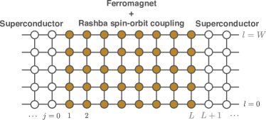
Figure 1: SFS junction on two-dimensional tight-binding model.

We solve the Gor’kov equation

$$\left[i\omega_{n}\hat{\tau}_{0}\hat{\sigma}_{0}-\sum_{\boldsymbol{r}_{1}}\left(\begin{array}[]{cc}\hat{H}_{\mathrm{N}}(\boldsymbol{r},\boldsymbol{r}_{1})&\hat{\Delta}(\boldsymbol{r},\boldsymbol{r}_{1})\\ -\hat{\Delta}^{\ast}(\boldsymbol{r},\boldsymbol{r}_{1})&-\hat{H}_{\mathrm{N}}^{\ast}(\boldsymbol{r},\boldsymbol{r}_{1})\end{array}\right)\right]$$ (16)

$$\times\check{G}_{\omega_{n}}(\boldsymbol{r}_{1},\boldsymbol{r}^{\prime})=\hat{\tau}_{0}\hat{\sigma}_{0}\delta(\boldsymbol{r}-\boldsymbol{r}^{\prime}),$$ (17)

$$\check{G}_{\omega_{n}}(\boldsymbol{r},\boldsymbol{r}^{\prime})=\left[\begin{array}[]{cc}\hat{G}_{\omega_{n}}(\boldsymbol{r},\boldsymbol{r}^{\prime})&\hat{F}_{\omega_{n}}(\boldsymbol{r},\boldsymbol{r}^{\prime})\\ -\hat{F}^{\ast}_{\omega_{n}}(\boldsymbol{r},\boldsymbol{r}^{\prime})&-\hat{G}^{\ast}_{\omega_{n}}(\boldsymbol{r},\boldsymbol{r}^{\prime})\end{array}\right],$$ (20)

by applying the lattice Green’s function technique Lee and Fisher (1981); Asano (2001), where $\tau_{0}$ is the unit matrix in particle-hole space, $\omega_{n}=(2n+1)\pi T$ is the fermionic Matsubara frequency, and $T$ is a temperature. The Josephson current in a ferromagnet $1<j<L$ expressed as

$$J(j)= -\frac{ie}{2}\,T\sum_{\omega_{n}}\sum_{m=1}^{W}\mathrm{Tr}\left[\hat{\tau}_{3}\check{T}_{+}\,\check{G}_{\omega_{n}}(\boldsymbol{r},\boldsymbol{r}+\boldsymbol{x})\right.$$

$$-\left.\hat{\tau}_{3}\check{T}_{-}\,\check{G}_{\omega_{n}}(\boldsymbol{r}+\boldsymbol{x},\boldsymbol{r})\right],$$ (21)

$$\check{T}_{\pm}= \left[\begin{array}[]{cc}-t\hat{\sigma}_{0}\mp i(\lambda/2)\hat{\sigma}_{2}&0\\ 0&t\hat{\sigma}_{0}\pm i(\lambda/2)\hat{\sigma}_{2}\end{array}\right],$$ (24)

is independent of $j$.

The pairing function with $s$-wave symmetry is decomposed into four components

$$\frac{1}{W}\sum_{m=1}^{W}\hat{F}_{\omega_{n}}(\boldsymbol{r},\boldsymbol{r})=\sum_{\nu=0}^{3}f_{\nu}(j)\hat{\sigma}_{\nu}i\hat{\sigma}_{2},$$ (25)

where $f_{0}$ is a spin-singlet component and $f_{j}$ with $j=1-3$ are spin-triplet components. In the clean limit, we also calculate pairing function with an odd-parity symmetry

$$\frac{1}{2W} \sum_{m=1}^{W}\hat{F}_{\omega_{n}}(\boldsymbol{r}+\boldsymbol{x},\boldsymbol{r})-\hat{F}_{\omega_{n}}(\boldsymbol{r}-\boldsymbol{x},\boldsymbol{r}),$$

$$=\sum_{\nu=0}^{3}f_{\nu}(j)\hat{\sigma}_{\nu}i\hat{\sigma}_{2}.$$ (26)

Throughout this paper, we fix several parameters as $W=20$, $\epsilon_{F}=2t$, $\Delta=0.005t$, and $T/T_{c}=0.1$. The exchange field is always in the perpendicular direction to the two-dimensional place $\boldsymbol{h}=h\boldsymbol{z}$.

III Clean limit

III.1 Josephson Current

We first discuss the numerical results of the Josephson current plotted as a function of the length of a ferromagnet $L$ in Fig. 2, where we fix the phase difference at $\varphi=\varphi_{L}-\varphi_{R}=0.5\pi$. Fig. 2(a) and (b) show the results in the absence of exchange potential $h=0$ and in the presence of an exchange potential $h=0.5t$, respectively. The Josephson current is normalized to $J_{0}=e\Delta$ throughout this paper. The amplitude of the Josephson current slightly decreases with the increase of $L$ because the pairing functions decay as $e^{-x/\xi^{C}_{T}}$ with $\xi^{C}_{T}=v_{F}/2\pi T$ for all pairing symmetry. We will discuss this point later on by using analytic expression of the pairing function obtained by solving Eilenberger equation. Since $h=0$ in Fig. 2(a), the junction corresponds to superconductor/normal-metal/superconductor junction. The results show that the spin-orbit interaction modifies the Josephson current very slightly. On the other hand in Fig. 2(b), the Josephson current oscillates as a function of $L$ because of the exchange potential. The period of the oscillations is described by $\xi^{C}_{h}=v_{F}/2h$ in weak spin-orbit interactions. When the spin-orbit interactions increase, the amplitude of the oscillations decreases. At $\lambda=0.5t$, the Josephson current is always positive at $\varphi=0.5\pi$. In the present calculation at $T/T_{c}=0.1$, the current-phase relationship (CPR) deviates slightly from sinusoidal function. Roughly speaking, the spin-orbit interaction stabilizes the 0 state rather than the $\pi$ state.

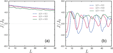
Figure 2: The Josephson current versus the length of a normal segment $L$ in the clean limit. (a): an SNS junction at $h=0$. (b): an SFS junction at $h=0.5t$.

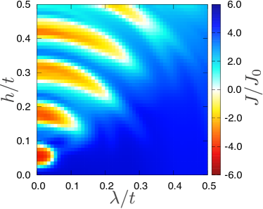
Figure 3: The Josephson current at $\varphi=0.5\pi$ and $L=50$ is plotted as a function of $h$ and $\lambda$ in the clean limit.

In Fig. 3, we show a phase diagram of the Josephson current at $\varphi=0.5\pi$ and $L=50$, where horizontal (vertical) axis indicates the amplitude of the spin-orbit interaction (exchange potential). The junction is in the 0 state for $J>0$ and is in the $\pi$ state for $J<0$. At $\lambda=0$, the Josephson current changes its sign with the increase of $h$, which indicates the 0-$\pi$ transition by the exchange potential. When we introduce the spin-orbit interaction, the 0-$\pi$ transitions is suppressed and the Josephson current is always positive. Roughly speaking $\pi$ state disappears for $\lambda>h$. We will discuss the reasons for disappearing the $\pi$ state under the strong spin-orbit interactions in the next subsection.

III.2 Pairing Functions

To analyze the characteristic behavior of the Josephson current, we solve the Eilenberger equation Eilenberger (1968) in a ferromagnet,

$$iv_{F}\hat{\boldsymbol{k}} \cdot\nabla_{\boldsymbol{r}}\check{g}+[\check{H}_{0}+\check{\Delta},\check{g}]_{-}=0,$$ (27)

$$\check{H}_{0}= \left(i\omega_{n}-\boldsymbol{h}\cdot\hat{\boldsymbol{\sigma}}\right)\hat{\tau}_{3}-\boldsymbol{\lambda}\times\hat{\boldsymbol{\sigma}}\cdot\hat{\boldsymbol{k}},$$ (28)

$$\check{\Delta}= i\hat{\Delta}\hat{\tau}_{1}.$$ (29)

To solve the Eilenberger equation, we apply the Riccati parameterization,

$$\check{g}=\left(\begin{matrix}\hat{N}&\hat{0}\\ \hat{0}&\underline{\hat{N}}\end{matrix}\right)\left(\begin{matrix}s_{\omega_{n}}(1-\hat{a}\hat{\underline{a}})&2\hat{a}\\ 2\hat{\underline{a}}&-s_{\omega_{n}}(1-\hat{\underline{a}}\hat{a})\end{matrix}\right),$$ (30)

where $s_{\omega_{n}}=\textrm{sgn}(\omega_{n})$. The two Riccati parameter are related to each other by $\hat{\underline{a}}(\boldsymbol{r},\hat{\boldsymbol{k}},\i\omega_{n})=\hat{\sigma}_{2}\hat{a}^{\ast}(\boldsymbol{r},-\hat{\boldsymbol{k}},i\omega_{n})\hat{\sigma}_{2}$. One of the Riccati parameter obeys

$$iv_{F} \hat{\boldsymbol{k}}\cdot\nabla\hat{a}+2i\omega_{n}\hat{a}-\boldsymbol{h}\cdot\hat{\boldsymbol{\sigma}}\hat{a}-\hat{a}\hat{\boldsymbol{\sigma}}\cdot\boldsymbol{h}-\hat{\boldsymbol{k}}\times\boldsymbol{\lambda}\cdot\hat{\boldsymbol{\sigma}}\hat{a}$$

$$+\hat{a}\hat{\boldsymbol{k}}\times\boldsymbol{\lambda}\cdot\hat{\boldsymbol{\sigma}}-i{\Delta}+i\hat{a}{\Delta}\hat{a}=0.$$ (31)

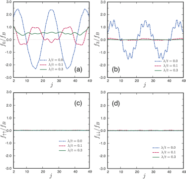
Figure 4: The spatial profile of the pairing functions at $L=50$ and $h=0.3t$ in the clean limit. The results for an $s$-wave symmetry in Eq. (25) are presented. (a) spin-singlet $f_{0}$, (b) opposite-spin-triplet $f_{3}$, (c) equal-spin-triplet $f_{\uparrow\uparrow}$, and (c) equal-spin-triplet $f_{\downarrow\downarrow}$

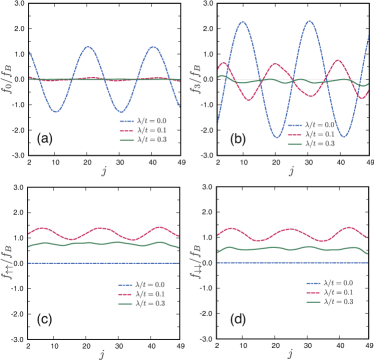
Figure 5: The results for an odd-parity symmetry in Eq. (26). The parameters are the same with those in Fig. 4. (a) spin-singlet $f_{0}$, (b) opposite-spin-triplet $f_{3}$, (c) equal-spin-triplet $f_{\uparrow\uparrow}$, and (c) equal-spin-triplet $f_{\downarrow\downarrow}$

Since $\Delta=0$ in a ferromagnet ($x>0$), it is possible to have an analytic solution of

$$\hat{a}(\boldsymbol{r},\hat{\boldsymbol{k}},i\omega_{n})=\sum_{\nu=0}^{3}a_{\nu}(\boldsymbol{r},\hat{\boldsymbol{k}},i\omega_{n})\hat{\sigma}_{\nu}.$$ (32)

The spin-singlet component satisfies

$$a_{0}(\boldsymbol{r},\hat{\boldsymbol{k}},i\omega_{n})=a_{0}(\boldsymbol{r},-\hat{\boldsymbol{k}},-i\omega_{n}),$$ (33)

and the three spin-triplet components satisfy

$$a_{j}(\boldsymbol{r},\hat{\boldsymbol{k}},i\omega_{n})=-a_{j}(\boldsymbol{r},-\hat{\boldsymbol{k}},-i\omega_{n}),$$ (34)

for $j=1-3$. For $\boldsymbol{h}=h\boldsymbol{z}$ and $\boldsymbol{\lambda}=\lambda\boldsymbol{z}$, we obtain the solution in two-dimension,

$$a_{0}= \frac{A_{0}}{V^{2}}\left[h^{2}\cos\left(\frac{2V}{v_{F_{x}}}x\right)+\lambda^{2}\right]e^{-\frac{2\omega_{n}}{v_{F_{x}}}x},$$ (35)

$$a_{\uparrow\uparrow}= a_{1}-ia_{2},$$ (36)

$$= \frac{A_{0}h\lambda}{V^{2}}(k_{y}+ik_{x})\left[1-\cos\left(\frac{2V}{v_{F_{x}}}x\right)\right]e^{-\frac{2\omega_{n}}{v_{F_{x}}}x},$$ (37)

$$a_{\downarrow\downarrow}= a_{1}+ia_{2},$$ (38)

$$= \frac{A_{0}h\lambda}{V^{2}}(-k_{y}+ik_{x})\left[1-\cos\left(\frac{2V}{v_{F_{x}}}x\right)\right]e^{-\frac{2\omega_{n}}{v_{F_{x}}}x},$$ (39)

$$a_{3}= i\frac{A_{0}h}{V}\sin\left(\frac{2V}{v_{F_{x}}}x\right)e^{-\frac{2\omega_{n}}{v_{F_{x}}}x},$$ (40)

where $V=\sqrt{h^{2}+\lambda^{2}}$, $v_{F_{x}}=k_{x}/m$ and $A_{0}=\Delta/(|\omega_{n}|+\sqrt{\omega_{n}^{2}+\Delta^{2}})$ is the solution in a uniform superconductor. At the interface of a superconductor and a ferromagnet $(x=0)$, we imposed a boundary condition of $a_{0}=A_{0}$ and $a_{j}=0$ for $j=1-3$. The decay length of all the components is basically given by the thermal coherence in the clean limit $\xi^{C}_{T}=v_{F}/2\pi T$. The spin-singlet component $a_{0}$ has two contributions: an oscillating term due to the exchange potential and a constant term due to the spin-orbit interaction. Eqs. (35)-(40) suggest that only a spin-singlet pair stays in an SNS junction. Thus the spin-orbit interaction does not affect the Josephson current so much as shown in Fig. 2(a). A opposite-spin-triplet component $a_{3}$ also oscillates in real space. The pairing function for equal-spin pairs $f_{\uparrow\uparrow}$ and $f_{\downarrow\downarrow}$ become finite in the presence of the spin-orbit unteraction and oscillate in real space. They, however, do not change their sign.

In Fig. 4, we show the numerical results of pairing function in the ferromagnet of an SFS junction on the tight-binding model, where $L=50$, $\varphi=0$, $h=0.3t$, and $\omega_{n}=0.02\Delta$. We first display the spatial profile of $s$-wave components in Eq. (25) for several choices of $\lambda$. The spin-singlet $s$-wave component $f_{0}$ in (a) oscillates and changes its sign in real space at $\lambda=0$. However, the spin-orbit interaction suppresses the sign change. As a result, $f_{0}$ is positive at any place for $\lambda=0.3t$. The opposite-spin-triplet component $f_{3}$ in (b) always changes its sing but is strongly suppressed by the spin-orbit interactions. We note that $f_{3}$ belongs to odd-frequency spin-triplet even-parity (OTE) symmetry class. The two equal-spin-triplet components in (c) and (d) are absent irrespective of $\lambda$. The analytical results of the Eilenberger equation predict these behavior well.

In Fig. 5, we display the spatial profile of the odd-parity components in Eq. (26) for several choices of $\lambda$. At $h=0$ and $\lambda=0$, the junction becomes an SNS junction and odd-parity components are absent in its normal segment. In the presence of the exchange potential, however, odd-parity opposite-spin Cooper pairs are generated in the clean junction because the exchange potential breaks inversion symmetry locally at the junction interface. The spin-singlet $s$-wave component $f_{0}$ in (a) oscillates and changes its sign in real space at $\lambda=0$. The spin-orbit interactions suppresses drastically such an odd-frequency spin-singlet odd-parity (OSO) component. The opposite-spin-triplet component $f_{3}$ in (b) belongs to even-frequency spin-triplet odd-parity (ETO) class shows similar behavior to $f_{0}$. Finally, the spin-orbit interactions generate two equal-spin-triplet components $f_{\uparrow\uparrow}$ and $f_{\downarrow\downarrow}$ as shown in (c) and (d), respectively. They oscillate slightly in real space but do not change their sign. The amplitude of such odd-parity equal spin components first increases with the increase of $\lambda$ then decrease in agreement with the analytical results in Eqs. (37) and (39). The spin-momentum locking due to the spin-orbit interaction explains such behaviors as we discuss in what follows.

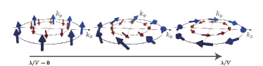
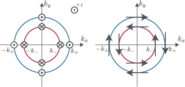
Figure 6: Schematic picture of spin-configuration on the Fermi surface. In Upper figure, the spins of an electron in the spin $\uparrow$ band are twisted by the spin-orbit interactions. The strong spin-orbit interaction fells spins down to a two-dimensional plane. In lower figure, spin configuration on the two Fermi surface are shown for the two limits: $h\gg\lambda$ on the left panel and $h\ll\lambda$ on the right panel.

Figure 6 shows the schematic spin structure on the Fermi surfaces. When the exchange potential is much larger than the spin-orbit interactions, spin of an electron aligns in each spin bands. The spin-orbit interactions twists the spin structure as shown in the upper middle figure. The strong spin-orbit interactions causes the spin-momentum locking as shown in the upper right figure. The spin configuration in the two limits are shown in the lower figure. The wavenumber $k_{\pm}$ in the figure are $k_{\pm}=k_{F}\pm h/v_{F}$ in the limit of $h\gg\lambda$ on the left and $k_{\pm}=k_{F}\pm\lambda/v_{F}$ in the limit of $h\ll\lambda$ on the right. At $h\gg\lambda$, a spin-singlet pair and an opposite-spin-triplet pair have a center-of-mass-momentum of $k_{+}+(-k_{-})=2h/v_{F}$ on the Fermi surface. As a result, these components oscillate and change their signs in real space Fulde and Ferrell (1964); Larkin and Ovchinnikov (1965). On the other hand, equal-spin-triplet components $f_{\uparrow\uparrow}$ ($f_{\downarrow\downarrow}$) do not have a center-of-mass-momentum because they consist of two electrons at $\pm k_{+}$ ($\pm k_{-}$). Thus equal-spin-triplet components do not change signs as shown in the results for $\lambda=0.1t$ in Fig. 5 (c) and (d).

In the opposite limit of $h\ll\lambda$, a spin-singlet Cooper pair does not have a center-of-mass-momentum in this case. The spin-momentum locking due to strong spin-orbit interactions stabilizes such a Cooper pair consisting of two electrons of time-reversal partners. Thus a spin-singlet Cooper pair does not oscillate in real space as shown in the results for $\lambda=0.3t$ in Fig. 4(a). Equal-spin-triplet pairs, on the other hand, have the center-of-mass-momentum $2\lambda/v_{F}$. In Fig. 5 (c) and (d), $f_{\sigma\sigma}$ for $\lambda=0.1t$ oscillate in real space. Since the spacial oscillations cost the energy, $f_{\sigma\sigma}$ for $\lambda=0.3t$ is smaller than that for $\lambda=0.1t$.

In the limit of $\lambda\gg h$, a spin-singlet Cooper pair is dominant in a ferromagnet and carries the Josephson current. The pairing function $f_{0}$ in Fig. 4 (a) does not changes sign. As a result, the 0 state is stable than the $\pi$ state for $\lambda>h$ as shown in Fig. 3.

IV Dirty regime

In the dirty limit, we switch on the random impurity potential in Eq. (9) in a ferromagnet, where the potential is given randomly in the range of $-V_{\mathrm{imp}}/2\leq v_{\boldsymbol{r}}V_{\mathrm{imp}}/2$. In the numerical simulation, we set $V_{\mathrm{imp}}=2t$, which results in the mean free path $\ell$ about five lattice constants. Since $\ell\ll L$, a ferromagnet is in the diffusive transport regime. The coherence length $\xi_{0}=v_{F}/\pi\Delta$ is estimated as twenty lattice constants at $\Delta=0.005t$. Thus the junction is in the dirty regime because of $\ell<\xi_{0}$. The Josephson current is first calculated for a single sample with a specific random impurity configuration. Then the results are averaged over $N_{\mathrm{s}}$ samples with different impurity configurations,

$$\langle J\rangle=\frac{1}{N_{\mathrm{s}}}\sum_{i=1}^{N_{\mathrm{s}}}J_{i}.$$ (41)

In this paper, we choose $N_{\mathrm{s}}$ as 100-500 in numerical simulation.

IV.1 Josephson Current

In Fig. 7, we show the ensemble average of the Josephson current as a function of the length of the ferromagnet, where we fix $\varphi=0.5\pi$, the exchange potential is absent in (a) and the exchange potential is $h=0.5t$ in (b). We confirmed that the current-phase relationship of ensemble aberaged Josephson current is sinusoidal. The decay length of the Josephson current in Fig. 7(a) is shorter than that in the clean limit in Fig. 2(a). It is well known in a diffusive normal metal that, the penetration length of a Cooper pairs is limited by $\xi^{D}_{T}=\sqrt{D/2\pi T}$. The Josephson current is almost free from spin-orbit interactions. The results of a SFS junction in Fig. 7(b) shows the oscillations and the sign change of the Josephson current at $\lambda=0.1t$. The large spin-orbit interaction suppresses the sign change of the Josephson current as show in the result for $\lambda=0.3t$.

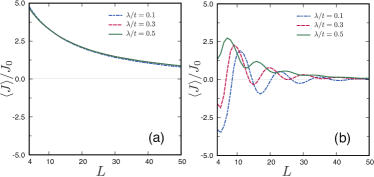
Figure 7: The Josephson current versus the length of a normal segment $L$ in the dirty limit. (a): an SNS junction at $h=0$. (b): an SFS junction at $h=0.5t$. The parameters here are the same as those in Fig. 2

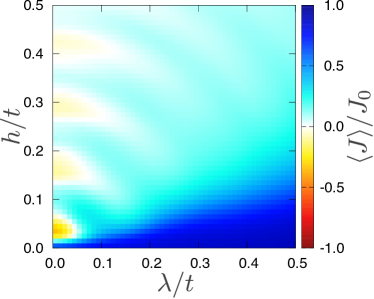
Figure 8: The Josephson current is plotted as a function of $h$ and $\lambda$ in the dirty regime. The parameters are the same as those in Fig. 3.

In Fig. 8, we plot the ensemble average of Josephson current at $\varphi=0.5\pi$ as a function of $h$ and $\lambda$. The results should be compared with those in Fig. 3. The amplitude of the Josephson current is suppressed by the impurity scatterings. Although the 0-$\pi$ transition can be seen at $\lambda=0$, the spin-orbit interaction suppresses the 0-$\pi$ transition. Such tendency is common in Figs. 3 and 8.

In the presence of impurities, however, the current-phase relation in a single sample deviates from the sinusoidal function as

$$J_{i}=J_{c}\sin(\varphi-\varphi_{i}),$$ (42)

where $\varphi_{i}$ is the phase shift depends on the random impurity configuration. The numerical results for several samples are shown in Fig. (11) in Appendix B with broken lines, where at $h=0.5t$ and $\lambda=0.5t$. The results show that the phase shift $\varphi_{i}$ depends on samples. The ensemble average of the results recovers the sinusoidal relationship as shown in a thick line in Fig. (11). The origin of the phase shift $\varphi_{i}$ is the breakdown of magnetic mirror reflection symmetry at the $xz$-plane by random potential. We discuss details of the symmetry breaking in Appendix A. Instead of explaining magnetic mirror reflection symmetry, we focus on a relation between the Josephson current in theories and that in experiments. In experiments, the Josephson current is measured in a specific sample of SFS junction. Since the Josephson effect is a result of the phase coherence of a quasiparticle developing over a ferromagnet, the Josephson current is not a self-averaged quantity. Therefore, the Josephson current calculated at a single sample $J_{i}$ corresponds to that at a single measurement in experiments. When the behavior of $\langle J\rangle$ and that of $J_{i}$ are different qualitatively from each other, $\langle J\rangle$ cannot predict a Josephson current measured in experiments Asano (2001). Therefore, $\langle J\rangle$ in Fig. 8 tell us only a tendency of $\varphi_{i}$ value. Namely, $\varphi_{i}\approx 0$ would be expected in experiments for $\lambda\gg h$. A previous paper Buzdin (2008) has discussed that the phase shit in the current-phase relationship $\varphi_{0}$ is tunable by applying the Zeeman field in the $y$ direction. The argument is valid only when a normal segment of a junction is in the ballistic transport regime and a junction geometry is symmetric under $y\to-y$.

IV.2 Pairing Functions

Although the ensemble average of the Josephson current in theories cannot predict the current-phase relationship measured in a real sample, the ensemble average of the pairing functions tells us characteristic features of the proximity effect. In Fig. 9, we show the spatial profile of the pairing functions in dirty regime, where $\varphi=0$, $h_{z}=0.5t$ and $L=50$. The parameters here are the same as those in Fig. 4. The singlet component $\langle f_{0}\rangle$ oscillates and changes its sign at $\lambda=0$ as shown in Fig. 9(a). At $\lambda=0.5t$, the spin-orbit interaction surpress the amplitude of oscillations. The similar tendency can be found also in the opposite-spin-triplet component $\langle f_{3}\rangle$ in (b). The equal-spin-triplet components $\langle f_{\sigma\sigma}\rangle$ are zero at $\lambda=0$. The amplitudes of such OTE pairs become finite and spatially uniform in the dirty regime as shown in in Fig. 9(c) and (d). Such characteristic features in the pairing functions can be seen also in a single sample shown in Fig. 12 in Appendix B. Although the results in a single sample show aperiodic oscillations due to random impurity potential, $f_{\sigma\sigma}$ in a single sample are positive everywhere as shown in Fig. 12 (c) and (d).

In the clean limit, the spin-momentum locking suppresses the equal-spin-triplet components as shown in Figs. 4 (c) and (d). In the dirty regime, however, the momentum is not a good quantum number. Equal-spin OTE pairs have the long-range property because random impurity scatterings release the spin-momentum locking.Bergeret and Tokatly (2013, 2014) At $\lambda>gh$, the results in Fig. 9 show that the most dominant pair in a ferromagnet belongs odd-frequency equal-spin-triplet $s$-wave symmetry class.

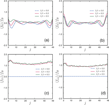
Figure 9: The spatial profile of the ensemble average of pairing function in the dirty regime. Only an $s$-wave component remains finite in the dirty regime. The parameters are the same as those in Fig. 4.

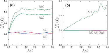
Figure 10: The pairing functions at the center of a ferromagnet $j=25$ are shown as a function of $\lambda$. (a): a strong ferromagnet at $h=0.5t$. (b): a half-metallic ferromagnet at $h=2.5t$.

We fix $j=25$ in Fig. 9 at a center of a ferromagnet and calculate the pairing functions as a function of $\lambda$. The results are presented in Fig. 10, where we choose $h=0.5t$ in (a) and $h=2.5t$ in (b). The pairing functions for opposite-spin pair $\langle f_{0}\rangle$ and $\langle f_{3}\rangle$ are insensitive to spin-orbit interactions. The amplitude of equal-spin pairs $\langle f_{\sigma\sigma}\rangle$ increases with the increase of $\lambda$ and saturate for $\lambda>2.0t$ in (a). Thus odd-frequency long-range components are dominant in a strong ferromagnet. When we increase the exchange potential to $h=2.5t$ in (b), a ferromagnet becomes half-metallic. Namely the ferromagnet is metallic for a spin-$\uparrow$ electron and is insulating for a spin-$\downarrow$ electron. In such a half-metal, only $\langle f_{\uparrow\uparrow}\rangle$ component survives and carries the Josephson current, which is very similar to the situation discussed in the previous papers. Braude and Nazarov (2007); Asano et al. (2007); Eschrig and Löfwander (2008).

V Conclusion

We theoretically study the proximity effect at a ferromagnetic semiconductor with Rashba spin-orbit interaction by solving the Gor’kov equation on a two-dimensional tight-binding lattice. The Green’s function is obtained numerically by using the lattice Green’s function technique. The exchange potential in a ferromagnet converts a spin-singlet Cooper pair to an opposite-spin-triplet Cooper pair. The spin-orbit interactions generate an equal-spin-triplet Cooper pair from an opposite-spin-triplet Cooper pair. The relative amplitudes of the four spin pairing components depend on the amplitude of spin-orbit interaction and the transport regime in a ferromagnet. In the presence of strong spin-orbit interaction, the spin-momentum locking stabilizes a conventional spin-singlet $s$-wave Cooper pair in the clean limit. In the dirty regime, on the other hand, the most dominant Cooper pair in a ferromagnet belongs to an odd-frequency equal-spin-triplet $s$-wave symmetry class. The impurity scatterings release the spin-momentum locking in the dirty regime.

Appendix A Magnetic mirror reflection symmetry

The Hamiltonian of a SFS junction is represented inn continuous space as

$$H(\boldsymbol{r})= \left[\begin{array}[]{cc}\xi_{\boldsymbol{r}}\hat{\sigma}_{0}&\Delta_{\boldsymbol{r}}\\ -\Delta^{\ast}_{\boldsymbol{r}}&-\xi_{\boldsymbol{r}}\hat{\sigma}_{0}\end{array}\right]+\left[\begin{array}[]{cc}H_{\mathrm{p}}(\boldsymbol{r})&0\\ 0&-H_{\mathrm{p}}^{\ast}(\boldsymbol{r})\end{array}\right],$$ (47)

$$\xi_{\boldsymbol{r}}= -\frac{\nabla^{2}}{2m}-\epsilon_{F},$$ (48)

$$\Delta_{\boldsymbol{r}}= \left[e^{i\varphi_{L}}\Theta(-x)+e^{i\varphi_{R}}\Theta(x-L)\right]\Delta i\sigma_{2},$$ (49)

$$H_{\mathrm{p}}= H_{\mathrm{h}}+H_{\textrm{so}}+H_{\mathrm{i}},$$ (50)

$$H_{\mathrm{h}}(\boldsymbol{r})= -\boldsymbol{h}\cdot\hat{\boldsymbol{\sigma}}\,\Theta(x)\,\Theta(L-x),$$ (51)

$$H_{\mathrm{so}}(\boldsymbol{r})= -i\lambda(\partial_{y}\hat{\sigma}_{1}-\partial_{x}\hat{\sigma}_{2})\Theta(x)\,\Theta(L-x),$$ (52)

$$H_{\mathrm{i}}(\boldsymbol{r})= \sum_{\boldsymbol{r}_{i}}v_{\boldsymbol{r}_{i}}\,\hat{\sigma}_{0}\delta(\boldsymbol{r}-\boldsymbol{r}_{i}).$$ (53)

The the eigen energy below the gap $E$ is a function on the phase difference between the two superconductors $\varphi-\varphi_{L}-\varphi_{R}$. When a relation $E(\varphi)=E(-\varphi)$ is satisfied, the Josephson current calculated by $J(\varphi)=e\partial_{\varphi}E$ is an odd function of $\varphi$. In such case, the junction is either 0 or $\pi$ states, which results in $J(0)=0$. The transformation of $\varphi\to-\varphi$ is realized by applying the complex conjugation to the Hamiltonian. Therefore, junction is either 0 or $\pi$ state when

$$H_{\mathrm{p}}=H_{\mathrm{p}}^{\ast},$$ (54)

is satisfied Sakurai et al. (2017). In the absence of spin-orbit interactions,

$$H_{\mathrm{h}}+H_{\mathrm{i}}=\left[H_{\mathrm{h}}+H_{\mathrm{i}}\right]^{\ast},$$ (55)

is satisfied when the magnetic moment is spatially uniform. It is always possible to describe the magnetic moment as $h_{x}\hat{\sigma}_{1}$ or $h_{z}\hat{\sigma}_{3}$ by rotating three axes in spin space in an appropriate way. The potentials in this paper are represented as

$$H_{\mathrm{p}}= h_{z}\hat{\sigma}_{3}-i\lambda\partial_{y}\sigma_{1}+i\lambda\partial_{x}\sigma_{2}+H_{\mathrm{i}}(\boldsymbol{r}),$$ (56)

$$H_{\textrm{p}}^{\ast}= h_{z}\hat{\sigma}_{3}+i\lambda\partial_{y}\sigma_{1}+i\lambda\partial_{x}\sigma_{2}+H_{\mathrm{i}}(\boldsymbol{r}).$$ (57)

Although the second term changes it sign under the complex conjugation, the additional transformation $y\to-y$ cancels the sign changing,

$$H_{\textrm{p}}^{\ast}\to h_{z}\hat{\sigma}_{3}-i\lambda\partial_{y}\sigma_{1}+i\lambda\partial_{x}\sigma_{2}+H_{\mathrm{i}}(x,-y).$$ (58)

Thus $E(\varphi)$ is an even function of $\varphi$ when $H_{\mathrm{i}}(x,-y)=H_{\mathrm{i}}(x,y)$ is satisfied. The impurity potential is $H_{\mathrm{i}}(x,-y)\neq H_{\mathrm{i}}(x,y)$ due to its random nature. In the presence of impurities, therefore, the energy of the junction takes its minimum at $\varphi=\varphi_{0}$ which is neither $\varphi=0$ nor $\varphi=\pi$. As a result, a single sample of Josephson junction with particular impurity configuration is $\varphi_{0}$ junction. When we average the Josephson current over a number of different samples, $\langle J(\varphi)\rangle$ show the sinusoidal relation satisfying $\langle J(0)\rangle=0$.

A paper Buzdin (2008) demonstrated tuning of $\varphi_{0}$ by introducing the Zeeman filed in the $y$ direction. In this case, $H_{\mathrm{h}}^{\prime}=h_{y}\hat{\sigma}_{2}$ changes its sign under the complex conjugation. Breaking magnetic mirror reflection symmetry by $h_{y}$ explains the mechanism of the tunable feature of $\varphi_{0}$.

Appendix B Numerical results for a single sample

In the dirty regime, calculated results for a single sample can be different from those of ensemble average. Here we present several results before ensemble averaging.

In Fig. 11, we show the current-phase relationship at $h=0.5t$ and $\lambda=0.5t$. The broken lines are the results calculated for several samples with different random configuration and deviate the sinusoidal function. A thick line corresponds to the ensemble average and is sinusoidal.

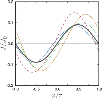
Figure 11: The current-phase relationship are shown for several samples with different impurity configuration at $h=0.5t$ and $\lambda=0.5t$. The Josephson current after ensemble averaging are plotted by a thick line.

Fig. 12 shows the spatial profile of the pairing function at $h_{z}=0.5t$. The results of ensemble average are shown in Fig. 9 All the components oscillate aperiodically in real space due to the random impurity potential. The opposite-spin components $f_{0}$ and $f_{3}$ change their sign, whereas the equal-spin components $f_{\sigma,\sigma}$ do not change their sign. Thus the results suggest the stability of equal-spin pairs in a single sample.

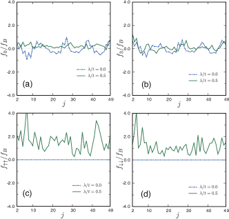
Figure 12: The spatial profile of the pairing function in a single sample.

References

- Bulaevskii et al. (1977) L. N. Bulaevskii, V. V. Kuzii, and A. A. Sobyanin, JETP Lett. 25, 290 (1977).
- Buzdin et al. (1982) A. I. Buzdin, L. N. Bulaevskii, and S. V. Panyukov, JETP lett 35, 178 (1982).
- Bergeret et al. (2001) F. S. Bergeret, A. F. Volkov, and K. B. Efetov, Phys. Rev. Lett. 86, 4096 (2001).
- Golubov et al. (2004) A. A. Golubov, M. Y. Kupriyanov, and E. Il’ichev, Rev. Mod. Phys. 76, 411 (2004).
- Ryazanov et al. (2001) V. V. Ryazanov, V. A. Oboznov, A. Y. Rusanov, A. V. Veretennikov, A. A. Golubov, and J. Aarts, Phys. Rev. Lett. 86, 2427 (2001).
- Kontos et al. (2002) T. Kontos, M. Aprili, J. Lesueur, F. Genêt, B. Stephanidis, and R. Boursier, Phys. Rev. Lett. 89, 137007 (2002).
- Keizer et al. (2006) R. S. Keizer, S. T. B. Goennenwein, T. M. Klapwijk, G. Miao, G. Xiao, and A. Gupta, Nature 439, 825 EP (2006).
- Anwar et al. (2010) M. S. Anwar, F. Czeschka, M. Hesselberth, M. Porcu, and J. Aarts, Phys. Rev. B 82, 100501 (2010).
- Khaire et al. (2010) T. S. Khaire, M. A. Khasawneh, W. P. Pratt, and N. O. Birge, Phys. Rev. Lett. 104, 137002 (2010).
- Robinson et al. (2010) J. W. A. Robinson, J. D. S. Witt, and M. G. Blamire, Science 329, 59 (2010), http://science.sciencemag.org/content/329/5987/59.full.pdf .
- Asano et al. (2007) Y. Asano, Y. Tanaka, and A. A. Golubov, Phys. Rev. Lett. 98, 107002 (2007).
- Braude and Nazarov (2007) V. Braude and Y. V. Nazarov, Phys. Rev. Lett. 98, 077003 (2007).
- Eschrig and Löfwander (2008) M. Eschrig and T. Löfwander, Nature Physics 4, 138 EP (2008), article.
- Eschrig (2015) M. Eschrig, Reports on Progress in Physics 78, 104501 (2015).
- Irie et al. (2014) H. Irie, Y. Harada, H. Sugiyama, and T. Akazaki, Phys. Rev. B 89, 165415 (2014).
- Takayanagi et al. (1995) H. Takayanagi, T. Akazaki, and J. Nitta, Phys. Rev. Lett. 75, 3533 (1995).
- Volkov and Takayanagi (1996) A. F. Volkov and H. Takayanagi, Phys. Rev. Lett. 76, 4026 (1996).
- Nakamura et al. (2018a) T. Nakamura, L. D. Anh, Y. Hashimoto, Y. Iwasaki, S. Ohya, M. Tanaka, and S. Katsumoto, Journal of Physics: Conference Series 969, 012036 (2018a).
- Nakamura et al. (2018b) T. Nakamura, L. D. Anh, Y. Hashimoto, S. Ohya, M. Tanaka, and S. Katsumoto, arXiv preprint arXiv:1806.08035 (2018b).
- Demler et al. (1997) E. A. Demler, G. B. Arnold, and M. R. Beasley, Phys. Rev. B 55, 15174 (1997).
- Buzdin (2008) A. Buzdin, Phys. Rev. Lett. 101, 107005 (2008).
- Liu et al. (2014) X. Liu, J. K. Jain, and C.-X. Liu, Phys. Rev. Lett. 113, 227002 (2014).
- Bergeret and Tokatly (2013) F. S. Bergeret and I. V. Tokatly, Phys. Rev. Lett. 110, 117003 (2013).
- Bergeret and Tokatly (2014) F. S. Bergeret and I. V. Tokatly, Phys. Rev. B 89, 134517 (2014).
- Jacobsen and Linder (2015) S. H. Jacobsen and J. Linder, Phys. Rev. B 92, 024501 (2015).
- Jacobsen et al. (2015) S. H. Jacobsen, J. A. Ouassou, and J. Linder, Phys. Rev. B 92, 024510 (2015).
- Costa et al. (2017) A. Costa, P. Högl, and J. Fabian, Phys. Rev. B 95, 024514 (2017).
- Mironov and Buzdin (2017) S. Mironov and A. Buzdin, Phys. Rev. Lett. 118, 077001 (2017).
- Lee and Fisher (1981) P. A. Lee and D. S. Fisher, Phys. Rev. Lett. 47, 882 (1981).
- Asano (2001) Y. Asano, Phys. Rev. B 63, 052512 (2001).
- Eilenberger (1968) G. Eilenberger, Zeitschrift für Physik A Hadrons and nuclei 214, 195 (1968).
- Fulde and Ferrell (1964) P. Fulde and R. A. Ferrell, Phys. Rev. 135, A550 (1964).
- Larkin and Ovchinnikov (1965) A. I. Larkin and Y. N. Ovchinnikov, Sov. Phys. JETP 20, 762 (1965).
- Sakurai et al. (2017) K. Sakurai, S. Ikegaya, and Y. Asano, Phys. Rev. B 96, 224514 (2017).