An introduction to fractal uncertainty principle

Abstract.

Fractal uncertainty principle states that no function can be localized in both position and frequency near a fractal set. This article provides a review of recent developments on the fractal uncertainty principle and of their applications to quantum chaos, including lower bounds on mass of eigenfunctions on negatively curved surfaces and spectral gaps on convex co-compact hyperbolic surfaces.

A fractal uncertainty principle (FUP) is a statement in harmonic analysis which can be vaguely formulated as follows (see Figure 1):

No function can be localized in both position and frequency

close to a fractal set.

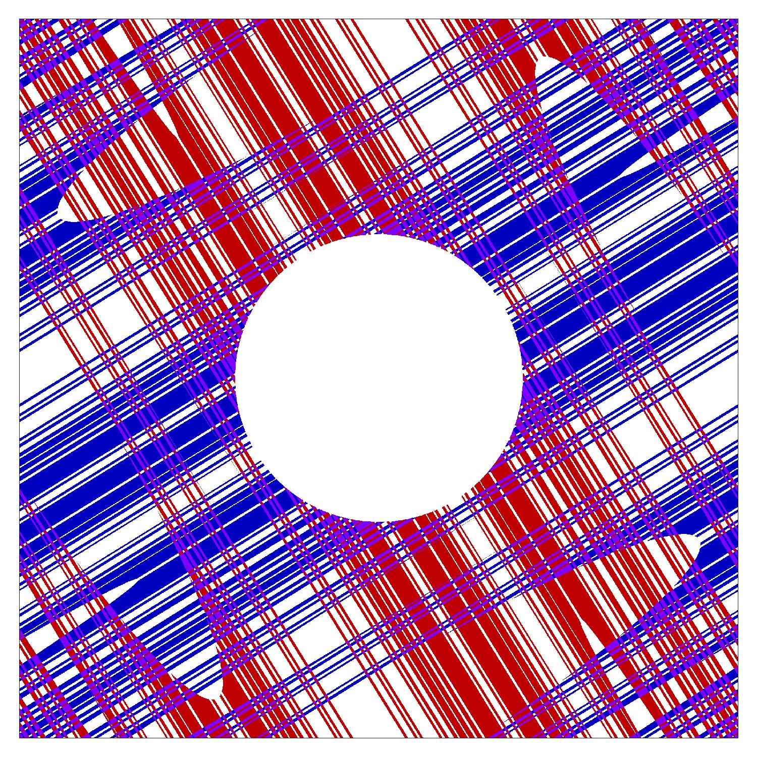
Figure 1. Left: a model situation to which FUP applies, with the blue/red sets corresponding to localization in position/frequency to a neighborhood of the middle third Cantor set. FUP states that no quantum wavefunction can be localized on both the red and the blue set. Right: a sample of two fractal sets used in applications of FUP to quantum chaos, consisting of trajectories of a hyperbolic dynamical system which do not cross some open set in forward/backward time direction – see Figure 4 below for details.

FUP has been successfully applied to problems in quantum chaos, which is the study of quantum systems in situations where the underlying classical system has chaotic behavior. See the reviews of Marklof [Ma06], Zelditch [Ze09], and Sarnak [Sa11] for an overview of this theory for compact systems, and the reviews of Nonnenmacher [No11] and Zworski [Zw17] for the case of noncompact, or open, systems. Applications of FUP include:

• lower bounds on mass of eigenfunctions, control for the Schrödinger equation, and exponential decay of damped waves on compact negatively curved surfaces (see §3.1);

• spectral gaps/exponential decay of waves on noncompact hyperbolic surfaces (see §3.2).

The present article is a broad review of various FUP statements and their applications. (A previous review article [Dy17] had a more detailed explanation of the proof of two of the results here, Theorems 2.16 and 3.1.) It is structured as follows:

• §2 gives the main FUP statements (Theorems 2.12–2.19), and briefly discusses the proofs. It also gives the definitions of fractal sets used throughout the article and describes Schottky limit sets, which are an important example. §§2.1–2.3 are the core of the article, the later parts of the article are often independent of each other;

• §3 describes applications of FUP to negatively curved surfaces;

• §4 considers the special class of discrete Cantor sets, giving a complete proof of FUP in this setting;

• §5 studies the relation of FUP to Fourier decay and additive energy improvements for fractal sets;

• §6 discusses generalizations of FUP to higher dimensions, which are largely not known at this point.

In addition to a review of known results, we state several open problems (Conjectures 4.4, 4.5, 5.7, 6.2, and 6.7) and provide figures with numerical evidence for both the known results and the conjectures. We also provide a more detailed exposition of a few topics:

• the relation between regular and porous sets (Proposition 2.10);

• reduction of FUP with a general phase to FUP for the Fourier transform (§2.5);

• a proof of FUP for discrete Cantor sets (§4.1);

• a proof of a special case of the recent result of Han–Schlag [HS18] in the setting of two-dimensional discrete Cantor sets (Proposition 6.9).

2. General results on FUP

2.1. Uncertainty principle

Before going fractal, we briefly review the standard uncertainty principle. Fix a small parameter $h>0$, called the semiclassical parameter, and consider the unitary semiclassical Fourier transform

$$\mathcal{F}_{h}:L^{2}(\mathbb{R})\to L^{2}(\mathbb{R}),\quad\mathcal{F}_{h}f(\xi)=(2\pi h)^{-1/2}\int_{\mathbb{R}}e^{-ix\xi/h}f(x)\,dx.$$ (2.1)

The version of the uncertainty principle we use is the following: for any $f\in L^{2}(\mathbb{R})$, either $f$ or its Fourier transform $\mathcal{F}_{h}f$ have little mass on the interval $[0,h]$. Specifically we have

$$\|\operatorname{1\hskip-2.75ptl}_{[0,h]}\mathcal{F}_{h}\operatorname{1\hskip-2.75ptl}_{[0,h]}\|_{L^{2}(\mathbb{R})\to L^{2}(\mathbb{R})}\leq h^{1/2}.$$ (2.2)

Here for $X\subset\mathbb{R}$, we denote by $\operatorname{1\hskip-2.75ptl}_{X}:L^{2}(\mathbb{R})\to L^{2}(\mathbb{R})$ the multiplication operator by the indicator function of $X$. One way to prove (2.2) is via Hölder’s inequality:

$$\|\operatorname{1\hskip-2.75ptl}_{[0,h]}\mathcal{F}_{h}\operatorname{1\hskip-2.75ptl}_{[0,h]}\|_{L^{2}\to L^{2}} \leq\|\operatorname{1\hskip-2.75ptl}_{[0,h]}\|_{L^{\infty}\to L^{2}}\cdot\|\mathcal{F}_{h}\|_{L^{1}\to L^{\infty}}\cdot\|\operatorname{1\hskip-2.75ptl}_{[0,h]}\|_{L^{2}\to L^{1}}$$ (2.3)

$$=h^{1/2}\cdot(2\pi h)^{-1/2}\cdot h^{1/2}\leq h^{1/2}.$$

A useful way to think about the norm bound (2.2) is as follows: if a function $f$ is supported in $[0,h]$, then the interval $[0,h]$ contains at most $h$ of the $L^{2}$ mass of $\mathcal{F}_{h}f$ (here we use the convention that the mass is the square of the $L^{2}$ norm).

The fractal uncertainty principle studied below concerns localization in position and frequency on more general sets:

Definition 2.1.

Let $X,Y\subset\mathbb{R}$ be $h$-dependent families of sets. We say that $X,Y$ satisfy uncertainty principle with exponent $\beta\geq 0$, if

$$\|\operatorname{1\hskip-2.75ptl}_{X}\mathcal{F}_{h}\operatorname{1\hskip-2.75ptl}_{Y}\|_{L^{2}(\mathbb{R})\to L^{2}(\mathbb{R})}=\mathcal{O}(h^{\beta})\quad\text{as }h\to 0.$$ (2.4)

2.2. Fractal sets

We now give two definitions of a ‘fractal set’ in $\mathbb{R}$. A more restrictive definition would be to require self-similarity under a group of transformations and this is true in some important examples (see §2.4 and §4). However, here we use a more general class of sets which have ‘fractal structure’ at every point and at a range of scales. To introduce those we use intervals, which are sets of the form $I=[a,b]\subset\mathbb{R}$ where $a<b$. The length of an interval is denoted by $|I|=b-a$.

The first definition we give is that of a regular set of dimension $\delta$, or $\delta$-regular set:

Definition 2.2.

Assume that $X\subset\mathbb{R}$ is a nonempty closed set and $0\leq\delta\leq 1$, $C_{R}\geq 1$, $0\leq\alpha_{\min}\leq\alpha_{\max}\leq\infty$. We say that $X$ is $\delta$-regular with constant $C_{R}$ on scales $\alpha_{\min}$ to $\alpha_{\max}$ if there exists a locally finite measure $\mu_{X}$ supported on $X$ such that for every interval $I$ centered at a point in $X$ and such that $\alpha_{\min}\leq|I|\leq\alpha_{\max}$ we have

$$C_{R}^{-1}|I|^{\delta}\leq\mu_{X}(I)\leq C_{R}|I|^{\delta}.$$ (2.5)

Remark 2.3.

In applications the precise value of $C_{R}$ is typically irrelevant: instead we consider a family of $\delta$-regular sets depending on a parameter $h\to 0$ and it is important that $C_{R}$ is independent of $h$.

Remark 2.4.

From (2.5) we deduce that $\mu_{X}(I)\leq 2C_{R}|I|^{\delta}$ for any interval $I$ (not necessarily centered on $X$) with $\alpha_{\min}\leq|I|\leq\alpha_{\max}$. Indeed, $I\cap X\subset I_{1}\cup I_{2}$ where $I_{j}$ is the interval of length $|I|$ centered at $x_{j}$ and $x_{1}=\min(I\cap X)$, $x_{2}=\max(I\cap X)$.

Example 2.5.

Here are some basic examples of $\delta$-regular sets (where $\alpha>0$):

1. the set $\{0\}$ is $0$-regular on scales $0$ to $\infty$ with constant 1;

2. the set $\mathbb{R}$ is $1$-regular on scales $0$ to $\infty$ with constant 1;

3. the set $[0,\alpha]$ is $0$-regular on scales $\alpha$ to $\infty$ with constant 2;

4. the set $[0,\alpha]$ is $1$-regular on scales $0$ to $\alpha$ with constant 2;

5. the set $\{0\}\cup[1,2]$ is not $\delta$-regular on scales 0 to 1 for any choice of $\delta,C_{R}$.

Examples (3) and (4) above demonstrate that the effective dimension of a set may depend on the scale: the interval $[0,\alpha]$ looks like a point on scales above $\alpha$ and like the entire real line on scales below $\alpha$. Example (5) shows that not every set has a dimension in the sense of Definition 2.2. On the other hand, one can show that no nonempty set can be $\delta$-regular on scales $0$ to 1 with two different values of $\delta$; that is, if a dimension in the sense of Definition 2.2 exists, then it is unique.

A more interesting example is given by

Example 2.6.

The middle third Cantor set

$$X:=\bigg{\{}\sum_{j=1}^{\infty}a_{j}3^{-j}\,\,\bigg{|}\,\,a_{1},a_{2},\dots\in\{0,2\}\bigg{\}}\ \subset\ [0,1]$$

is $\log_{3}2$-regular on scales 0 to 1 with constant 2. (To show this we can use that $\mu(I)=2^{-j}$ for any interval $I$ of length $2\cdot 3^{-j}$, $j\in\mathbb{N}_{0}$, centered at a point in $X$, where $\mu$ is the Cantor measure.)

Our second definition of a ‘fractal set’ is more general. Rather than requiring the same dimension at each point it asks for the set to have gaps, or pores, and is a quantitative version of being nowhere dense:

Definition 2.7.

Assume that $X\subset\mathbb{R}$ is a closed set and $\nu>0$, $0\leq\alpha_{\min}\leq\alpha_{\max}\leq\infty$. We say that $X$ is $\nu$-porous on scales $\alpha_{\min}$ to $\alpha_{\max}$ if for each interval $I$ such that $\alpha_{\min}\leq|I|\leq\alpha_{\max}$, there exists an interval $J\subset I$ such that $|J|=\nu|I|$ and $X\cap J=\emptyset$.

Remark 2.8.

As with the regularity constant $C_{R}$, the precise value of $\nu$ will typically not be of importance.

Example 2.9.

The middle third Cantor set is $\nu$-porous on scales 0 to $\infty$ for any $\nu<{1\over 5}$.

The next proposition establishes a partial equivalence between the notions of regularity and porosity by showing that porous sets can be characterized as subsets of $\delta$-regular sets with $\delta<1$:

Proposition 2.10.

Fix $0\leq\alpha_{\min}\leq\alpha_{\max}\leq\infty$.

1. Assume that $X$ is $\delta$-regular with constant $C_{R}$ on scales $\alpha_{\min}$ to $\alpha_{\max}$, and $\delta<1$. Then $X$ is $\nu$-porous on scales $C\alpha_{\min}$ to $\alpha_{\max}$ where $\nu>0$ and $C$ depend only on $\delta,C_{R}$.

2. Assume that $X$ is $\nu$-porous on scales $\alpha_{\min}$ to $\alpha_{\max}$. Then $X$ is contained in some set $Y\subset\mathbb{R}$ which is $\delta$-regular with constant $C_{R}$ on scales $\alpha_{\min}$ to $\alpha_{\max}$ where $\delta<1$ and $C_{R}$ depend only on $\nu$.

Proof.

1. Fix $T\in\mathbb{N}$ to be chosen later depending on $\delta,C_{R}$ and put $\nu:=(3T)^{-1}$, $C:=3T$. Let $I$ be an interval with $C\alpha_{\min}\leq|I|\leq\alpha_{\max}$. We partition $I$ into $T$ intervals $I_{1},\dots,I_{T}$, each of length $|I|/T$. We argue by contradiction, assuming that each interval $J\subset I$ with $|J|=\nu|I|$ intersects $X$. Then this applies to the middle third of each of the intervals $I_{r}$, implying that the interior of $I_{r}$ contains an interval $I^{\prime}_{r}$ of length $|I|/C$ centered at a point in $X$. We now use that $\bigsqcup_{r}I_{r}^{\prime}\subset I$ and write using $\delta$-regularity of $X$

$$TC_{R}^{-1}\Big{(}{|I|\over 3T}\Big{)}^{\delta}\leq\sum_{r=1}^{T}\mu(I^{\prime}_{r})\leq\mu(I)\leq 2C_{R}|I|^{\delta}.$$

Since $\delta<1$ we may choose $T$ so that $T^{1-\delta}>6C_{R}^{2}$, giving a contradiction.

2. We only provide a sketch, referring to [DJ18b, Lemma 5.4] for details. Fix $L\in\mathbb{N}$ such that $L>2/\nu$. Assume for simplicity that $\alpha_{\min}=0$, $\alpha_{\max}=1$, and $X$ is contained in an interval $I$ with $|I|=1$. We partition $I$ into $L$ intervals $I_{1},\dots,I_{L}$, each of length $|I|/L<\nu/2$. By the porosity property there exists $\ell_{0}$ such that $I_{\ell_{0}}\cap X=\emptyset$. Then $X$ is contained in the union $Y_{1}:=\bigcup_{\ell\neq\ell_{0}}I_{\ell}$. We now partition each of the intervals $I_{\ell}$, $\ell\neq\ell_{0}$ into $L$ pieces, one of which will again not intersect $X$ by the porosity property and will be removed. This gives a covering of $X$ by a union $Y_{2}$ of $(L-1)^{2}$ intervals, each of length $L^{-2}$. Repeating the process we construct sets $Y_{1}\supset Y_{2}\supset\dots$ covering $X$ and the intersection $Y:=\bigcap_{k}Y_{k}$ is a ‘Cantor-like’ set which is $\delta$-regular with $\delta:=\log_{L}(L-1)<1$. ∎

Many natural constructions give sets which are regular/porous on scales 0 to 1. Neighborhoods of such sets of size $h\ll 1$ (to which FUP will be typically applied) are then regular/porous on scales $Ch$ to $1$:

Proposition 2.11.

Let $0<h<1$.

1. Assume that $X$ is $\delta$-regular on scales 0 to 1 with constant $C_{R}$. Then the neighborhood

$$X(h):=X+[-h,h]$$

is $\delta$-regular on scales $h$ to $1$ with constant $C^{\prime}_{R}$, where $C^{\prime}_{R}$ depends only on $C_{R}$.

2. Assume that $X$ is $\nu$-porous on scales 0 to 1. Then $X(h)$ is $\nu\over 3$-porous on scales ${3\over\nu}h$ to 1.

Proof.

1. See [BD18, Lemma 2.3].

2. Take an interval $I$ such that ${3\over\nu}h\leq|I|\leq 1$. By the porosity of $X$ there exists an interval $J\subset I$ with $|J|=\nu|I|\geq 3h$ and $J\cap X=\emptyset$. Let $J^{\prime}$ be the middle third of $J$, then $J^{\prime}\subset I$, $|J^{\prime}|={\nu\over 3}|I|$, and $J^{\prime}\cap X(h)=\emptyset$. ∎

2.3. Statement of FUP

The fractal uncertainty principle gives a partial answer to the following question:

Fix $\delta\in[0,1]$ and $C_{R}\geq 1$. What is the largest value of $\beta$ such that (2.4) holds

for all $h$-dependent families of sets $X,Y\subset[0,1]$

which are $\delta$-regular with constant $C_{R}$ on scales $h$ to 1?

One way to establish (2.4) is to use the following volume (Lebesgue measure) bound: if $X\subset[0,1]$ is $\delta$-regular on scales $h$ to 1 with constant $C_{R}$, then for some $C=C(\delta,C_{R})$

$$\operatorname{vol}(X)\leq Ch^{1-\delta}.$$ (2.6)

See [BD18, Lemma 2.9] for the proof.

Using (2.6) and arguing as in (2.3), we see that (2.4) holds for $\beta={1\over 2}-\delta$:

$$\|\operatorname{1\hskip-2.75ptl}_{X}\mathcal{F}_{h}\operatorname{1\hskip-2.75ptl}_{Y}\|_{L^{2}\to L^{2}}\leq h^{-1/2}\sqrt{\operatorname{vol}(X)\operatorname{vol}(Y)}\leq Ch^{1/2-\delta}.$$

It also holds for $\beta=0$ since $\mathcal{F}_{h}$ is unitary. Therefore, we get the basic FUP exponent

$$\beta_{0}=\max\Big{(}0,{1\over 2}-\delta\Big{)}.$$ (2.7)

Note that for $0\leq\delta\leq 1$, we have as $h\to 0$

$$\|\operatorname{1\hskip-2.75ptl}_{[0,h^{1-\delta}]}\mathcal{F}_{h}\operatorname{1\hskip-2.75ptl}_{[0,h^{1-\delta}]}\|_{L^{2}\to L^{2}}\sim h^{\max(0,1/2-\delta)}$$

as can be seen by applying the operator on the left-hand side to a function of the form $\chi(x/h^{1-\delta})$ where $\chi\in C^{\infty}_{\mathrm{c}}((0,1))$. This shows that (2.7) cannot be improved if we only use the volumes of $X,Y$. Instead Theorems 2.12–2.16 below take advantage of the fractal structure of $X$ and/or $Y$ at many different points and at different scales. Also, by taking $X=Y=[0,1]$ or $X=Y=[0,h]$ we see that (2.7) is sharp when $\delta=0$ or $\delta=1$.

We now present the central result of this article which is a fractal uncertainty principle improving over (2.7) in the entire range $0<\delta<1$. Improving over $\beta=0$ and over $\beta={1\over 2}-\delta$ is done using different methods, so we split the result into two statements:

Theorem 2.12.

[BD18, Theorem 4] Fix $\delta<1$ and $C_{R}\geq 1$. Then there exists

$$\beta=\beta(\delta,C_{R})>0$$ (2.8)

such that (2.4) holds for all $h$-dependent families of sets $X,Y\subset[0,1]$ which are $\delta$-regular with constant $C_{R}$ on scales $h$ to $1$.

Theorem 2.13.

[DJ18a, Theorem 1] Fix $\delta>0$ and $C_{R}\geq 1$. Then there exists

$$\beta=\beta(\delta,C_{R})>{1\over 2}-\delta$$ (2.9)

such that (2.4) holds for all $h$-dependent families of sets $X,Y\subset[0,1]$ which are $\delta$-regular with constant $C_{R}$ on scales $h$ to $1$.

Remark 2.14.

There exist estimates on the size of the improvement $\beta-\max(0,{1\over 2}-\delta)$ in terms of $\delta,C_{R}$, see [DJ18a] for (2.9) and Jin–Zhang [JZ17] for (2.8).

Remark 2.15.

More results on FUP in special settings (Cantor sets, Schottky limit sets) are described below in §4 and §5.1 and higher dimensions are discussed in §6.

An application of Theorem 2.12 and Proposition 2.10 is the following version of FUP for porous sets:

Theorem 2.16.

Fix $\nu>0$. Then there exists $\beta=\beta(\nu)>0$ such that (2.4) holds for all $h$-dependent families of sets $X,Y\subset[0,1]$ which are $\nu$-porous on scales $h$ to $1$.

We now briefly discuss the proofs of Theorem 2.12–2.13. See also [Dy17, §4] for a more detailed expository treatment of Theorem 2.12.

To prove Theorem 2.12 we rewrite the estimate (2.4) as follows:

$$f\in L^{2}(\mathbb{R}),\ \operatorname{supp}\hat{f}\subset h^{-1}\cdot Y\quad\Longrightarrow\quad\|\operatorname{1\hskip-2.75ptl}_{X}f\|_{L^{2}}\leq Ch^{\beta}\|f\|_{L^{2}}.$$ (2.10)

The proof of (2.10) proceeds by iteration on scales $1,{1\over 2},\dots,2^{-j},\dots,h$. At each scale $\alpha$ we use the porosity of $X$ to find many intervals of size $\sim\alpha$ which do not intersect $X$; denote their union by $U_{\alpha}$. The upper bound (2.10) then follows from a lower bound on the mass of $f$ on $U_{\alpha}$. Such lower bounds are known if $f$ belongs to a quasi-analytic class, i.e. if the Fourier transform $\hat{f}$ decays fast enough. (For instance if $\hat{f}$ decays exponentially fast then $f$ is real-analytic and cannot identically vanish on any interval.)

To convert the Fourier support condition (2.10) to a Fourier decay statement we convolve $f$ with a function $\psi$ which is compactly supported (so that we do not lose the ability to bound the norm of $f$ on an interval) and has Fourier transform decaying almost exponentially fast on the set $h^{-1}\cdot Y$. The function $\psi$ is constructed using the Beurling–Malliavin theorem [BM62] with a weight tailored to the set $Y$, whose existence uses the fact that $Y$ is $\delta$-regular with $\delta<1$. (One does not actually need the full strength of the Beurling–Malliavin theorem as explained in [JZ17]). In particular, we use the fact that $X,Y$ are ‘not too big’ in two different ways: the porosity property and a quantitative sparsity following from (2.5) when $\delta<1$. In the much simpler setting of arithmetic Cantor sets these two properties appear in the proof of Lemma 4.7.

The proof of Theorem 2.13 is inspired by the works of Dolgopyat [Do98] and Naud [Na05]. Note that if we replace $e^{-ix\xi/h}$ in the definition of the Fourier transform $\mathcal{F}_{h}$ by 1, then the norm (2.4) is asymptotic to $h^{1/2-\delta}$ (assuming $\operatorname{vol}(X)\sim\operatorname{vol}(Y)\sim h^{1-\delta}$). Thus to get an improvement we need to use cancellations coming from the phase in the Fourier transform. Using that $\delta>0$ (that is, $X,Y$ are ‘not too small’) we can find many quadruples of points $x_{1},x_{2}\in X$, $y_{1},y_{2}\in Y$ such that the phase factor $e^{i(x_{1}-x_{2})(y_{1}-y_{2})/h}$ is far from 1. These quadruples cause cancellations which lead to (2.4) with $\beta>{1\over 2}-\delta$. In general one has to be careful at exploiting the cancellations to make sure they compound on many different scales; the argument is again much simpler in the setting of arithmetic Cantor sets, see Lemma 4.8.

2.4. Schottky limit sets

Many natural fractal sets are constructed using iterated function systems. Here we briefly present a special class of these, Schottky limit sets, which naturally arise in the spectral gap problem on hyperbolic surfaces (see §3.2 below). We refer to [BD17, §2] and [Bo16, §15.1] for more details.

Schottky limit sets are generated by fractional linear (Möbius) transformations

$$x\mapsto\gamma.x={ax+b\over cx+d},\quad\gamma=\begin{pmatrix}a&b\\ c&d\end{pmatrix}\in\operatorname{SL}_{2}(\mathbb{R}),\quad x\in\dot{\mathbb{R}}:=\mathbb{R}\cup\{\infty\}.$$ (2.11)

More precisely, we:

Figure 2. An example of a Schottky limit set, picturing the sets in (2.12) for $n=1,2,3$. The Schottky data are as follows: $I_{1}=[-4,-3]$, $I_{2}=[-2,-1]$, $I_{3}=[0,1]$, $I_{4}=[2,3]$, $\gamma_{1}=\left(\begin{smallmatrix}7&-3\\ -2&1\end{smallmatrix}\right)$, $\gamma_{2}=\left(\begin{smallmatrix}3&-7\\ -2&5\end{smallmatrix}\right)$. The bottom row is a union of 36 intervals, illustrating the difficulty of plotting a ‘nonlinear’ fractal set.

• fix a collection of nonintersecting intervals $I_{1},\dots,I_{2r}\subset\mathbb{R}$, where $r\geq 1$;

• denote $\mathcal{A}:=\{1,\dots,2r\}$ and for each $w\in\mathcal{A}$, define $\overline{w}:=w+r$ if $w\leq r$ and $\overline{w}:=w-r$ otherwise;

• fix transformations $\gamma_{1},\dots,\gamma_{2r}\in\operatorname{SL}_{2}(\mathbb{R})$ such that for all $w\in\mathcal{A}$ we have $\gamma_{\overline{w}}=\gamma_{w}^{-1}$ and the image of $\dot{\mathbb{R}}\setminus I_{\overline{w}}$ under $\gamma_{w}$ is the interior of $I_{w}$;

• for $n\in\mathbb{N}$, define the set $\mathcal{W}_{n}$ consisting of words $\mathbf{w}=w_{1}\dots w_{n}$ such that $w_{j+1}\neq\overline{w_{j}}$ for all $j=1,\dots,n-1$;

• for each word $\mathbf{w}=w_{1}\dots w_{n}\in\mathcal{W}_{n}$ define the interval $I_{\mathbf{w}}=\gamma_{w_{1}}\dots\gamma_{w_{n-1}}(I_{w_{n}})$. Since $I_{w_{n}}\subset\dot{\mathbb{R}}\setminus I_{\overline{w_{n-1}}}$ we have $I_{\mathbf{w}}\subset I_{w_{1}\dots w_{n-1}}$, so the collection of intervals $I_{\mathbf{w}}$ forms a tree (see Figure 2);

• the limit set $X$ is now defined as the intersection of a decreasing family of sets

  $$X:=\bigcap_{n}\bigsqcup_{\mathbf{w}\in\mathcal{W}_{n}}I_{\mathbf{w}}.$$ (2.12)

The transformations $\gamma_{1},\dots,\gamma_{r}$ generate a discrete free subgroup $\Gamma\subset\operatorname{SL}_{2}(\mathbb{R})$, called a Schottky group, and $\Gamma$ acts on the limit set $X$. For $r=1$ the set $X$ consists of just two points, so we henceforth assume $r\geq 2$. In this case $X$ is $\delta$-regular for some $\delta\in(0,1)$, see [BD17, Lemma 2.12]. The corresponding measure in Definition 2.2 is the Patterson–Sullivan measure on $X$, see [Bo16, §14.1].

Schottky limit sets give a fundamental example of ‘nonlinear’ fractal sets in the sense that the transformations generating them are nonlinear (as opposed to linear Cantor sets such as those studied in §4 below). This often complicates their analysis, however this nonlinearity is sometimes also useful – in particular it implies Fourier decay for Schottky limit sets while linear Cantor sets do not have this property, see Theorem 5.2.

2.5. FUP with a general phase

In applications we often need a more general version of FUP, with the Fourier transform (2.1) replaced by an oscillatory integral operator

$$\mathcal{B}_{h}f(x)=(2\pi h)^{-1/2}\int_{\mathbb{R}}e^{i\Phi(x,y)/h}b(x,y)f(y)\,dy.$$ (2.13)

Here the phase function $\Phi\in C^{\infty}(U;\mathbb{R})$ satisfies the nondegeneracy condition

$$\partial^{2}_{xy}\Phi(x,y)\neq 0\quad\text{on}\quad U,$$ (2.14)

$U\subset\mathbb{R}^{2}$ is an open set, and the amplitude $b$ lies in $C^{\infty}_{\mathrm{c}}(U)$. The nondegeneracy condition ensures that the norm $\|\mathcal{B}_{h}\|_{L^{2}\to L^{2}}$ is bounded uniformly as $h\to 0$. The phase function used in applications to hyperbolic surfaces in §3 is

$$\Phi(x,y)=\log|x-y|,\quad U=\{(x,y)\in\mathbb{R}^{2}\mid x\neq y\},$$ (2.15)

and FUP with this phase function is called the hyperbolic FUP.

The following results generalize Theorems 2.12–2.16. In all of these we assume that $\Phi$ satisfies (2.14); the constant $\beta$ depends only on $\delta,C_{R}$ (or $\nu$ in the case of Theorem 2.19) and the constant $C$ additionally depends on $\Phi,b$. However, the values of $\beta$ obtained in Theorems 2.17,2.19 below are smaller than the ones in Theorems 2.12,2.16. Since $b$ is compactly supported we may remove the condition $X,Y\subset[0,1]$.

Theorem 2.17.

[BD18, Proposition 4.3] Fix $\delta<1$ and $C_{R}\geq 1$. Then there exists

$$\beta=\beta(\delta,C_{R})>0$$ (2.16)

such that for all $X,Y\subset\mathbb{R}$ which are $\delta$-regular with constant $C_{R}$ on scales $h$ to $1$ we have

$$\|\operatorname{1\hskip-2.75ptl}_{X}\mathcal{B}_{h}\operatorname{1\hskip-2.75ptl}_{Y}\|_{L^{2}(\mathbb{R})\to L^{2}(\mathbb{R})}\leq Ch^{\beta}.$$ (2.17)

Theorem 2.18.

[DJ18a] Fix $\delta>0$ and $C_{R}\geq 1$. Then there exists

$$\beta=\beta(\delta,C_{R})>{1\over 2}-\delta$$ (2.18)

such that (2.17) holds for all $X,Y\subset\mathbb{R}$ which are $\delta$-regular with constant $C_{R}$ on scales $h$ to $1$.

Theorem 2.19.

Fix $\nu>0$. Then there exists $\beta=\beta(\nu)>0$ such that (2.17) holds for all $h$-dependent families of sets $X,Y\subset\mathbb{R}$ which are $\nu$-porous on scales $h$ to $1$.

We give an informal explanation for how to reduce Theorem 2.17 to the case of Fourier transform, Theorem 2.12. (For Theorem 2.18, the argument in [DJ18a] handles the case of a general phase directly.) The argument we give below gives $\beta$ which depends on $\Phi$ in addition to $\delta,C_{R}$, but it can be modified to remove this dependence.

We first consider the case of the Fourier transform phase $\Phi(x,y)=-xy$ and arbitrary amplitude $b\in C^{\infty}_{\mathrm{c}}(\mathbb{R}^{2})$. Fix $\rho\in(0,1)$ which is very close to 1. For each $f\in L^{2}(\mathbb{R})$, the function $\mathcal{B}_{h}\operatorname{1\hskip-2.75ptl}_{Y}f$ is localized to semiclassical frequencies in the neighborhood $Y(h^{\rho})$ in the following sense: for all $N$

$$\|\operatorname{1\hskip-2.75ptl}_{\mathbb{R}\setminus Y(h^{\rho})}\mathcal{F}_{h}^{-1}\mathcal{B}_{h}\operatorname{1\hskip-2.75ptl}_{Y}f\|_{L^{2}(\mathbb{R})}\leq C_{N}h^{N}\|f\|_{L^{2}(\mathbb{R})}.$$ (2.19)

Indeed, the operator $\mathcal{F}_{h}^{-1}\mathcal{B}_{h}$ has integral kernel

$$K(x,y)=(2\pi h)^{-1}\int_{\mathbb{R}}e^{i(x-y)w/h}b(w,y)\,dw.$$

Repeated integration by parts shows that $|K(x,y)|\leq C_{N}h^{-1}(1+|x-y|/h)^{-N}$ for all $N$, which implies (2.19).

Armed with (2.19), we may replace $u:=\mathcal{B}_{h}\operatorname{1\hskip-2.75ptl}_{Y}f$ by $\mathcal{F}_{h}\operatorname{1\hskip-2.75ptl}_{Y(h^{\rho})}\mathcal{F}_{h}^{-1}u$ in (2.17), which then reduces to

$$\|\operatorname{1\hskip-2.75ptl}_{X}\mathcal{F}_{h}\operatorname{1\hskip-2.75ptl}_{Y(h^{\rho})}\|_{L^{2}(\mathbb{R})\to L^{2}(\mathbb{R})}\leq Ch^{\beta}.$$ (2.20)

Now (2.20) with $\rho:=1$ follows from FUP for Fourier transform, Theorem 2.12, since $Y(h)$ is still $\delta$-regular on scales $Ch$ to 1 similarly to Proposition 2.11. For $\rho<1$ we may write $Y(h^{\rho})$ as a union of $\sim h^{\rho-1}$ shifted copies of the set $Y(h)$, which bounds the left-hand side of (2.20) by $Ch^{\beta+\rho-1}$. It remains to take $\rho$ close enough to 1 so that $\beta+\rho-1>0$.

We now explain how to handle the case of a general phase $\Phi$ satisfying (2.14), using almost orthogonality and a linearization argument. We first take $\rho<1$ close to 1 and replace the set $X$ by a smoothened version of its neighborhood $X(h^{\rho/2})$ in (2.17). More precisely, take a function

$$\chi\in C^{\infty}(\mathbb{R};[0,1]),\quad\operatorname{supp}\chi\subset X(h^{\rho/2}),\quad\operatorname{supp}(1-\chi)\cap X=\emptyset$$

which satisfies the derivative bounds for all $N$

$$\sup|\partial^{N}\chi|\leq C_{N}h^{-\rho N/2}.$$ (2.21)

Then it suffices to show the bound

$$\|\chi\mathcal{B}_{h}\operatorname{1\hskip-2.75ptl}_{Y}\|_{L^{2}(\mathbb{R})\to L^{2}(\mathbb{R})}\leq Ch^{\beta}.$$ (2.22)

The bound (2.22) is stronger than (2.17) and thus appears harder to prove. However, if the sets $Y_{1},Y_{2}\subset\mathbb{R}$ are at distance $\geq h^{1/2}$, then we have the almost orthogonality estimate for all $N$

$$\|(\chi\mathcal{B}_{h}\operatorname{1\hskip-2.75ptl}_{Y_{1}})^{*}\chi\mathcal{B}_{h}\operatorname{1\hskip-2.75ptl}_{Y_{2}}\|_{L^{2}(\mathbb{R})\to L^{2}(\mathbb{R})}\leq C_{N}h^{N}.$$ (2.23)

To show (2.23) we write the integral kernel of the operator $\mathcal{B}_{h}^{*}\chi^{2}\mathcal{B}_{h}$,

$$K_{1}(x,y)=(2\pi h)^{-1}\int_{\mathbb{R}}e^{i(\Phi(w,y)-\Phi(w,x))/h}\overline{b(w,x)}b(w,y)\chi(w)^{2}\,dw.$$

We repeatedly integrate by parts in $w$. Each integration by parts gives a gain of $h/|x-y|$ from the phase, using the inequality

$$|\partial_{w}(\Phi(w,x)-\Phi(w,y))|\geq C^{-1}|x-y|$$

which is a consequence of (2.14). On the other hand differentiating the $\chi^{2}(w)$ factor we get a $h^{\rho/2}$ loss by (2.21). For $|x-y|\geq h^{1/2}$ we get an $h^{(1-\rho)/2}$ improvement with each integration by parts, giving (2.23).

Now, we split $Y$ into a disjoint union of clusters $Y_{j}$, each contained in an interval of size $h^{1/2}$. Using (2.23) and the Cotlar–Stein Theorem [Zw12, Theorem C.5] we see that it suffices to show the norm bound for each individual cluster

$$\|\chi\mathcal{B}_{h}\operatorname{1\hskip-2.75ptl}_{Y_{j}}\|_{L^{2}(\mathbb{R})\to L^{2}(\mathbb{R})}\leq Ch^{\beta}.$$ (2.24)

For simplicity we assume that $Y_{j}=Y\cap[0,h^{1/2}]$. Composing $\mathcal{B}_{h}$ with the isometry $Tf(y)=h^{-1/4}f(y/h^{1/2})$ we get the operator

$$\widetilde{\mathcal{B}}_{h}f(x)=(2\pi\sqrt{h})^{-1/2}\int_{\mathbb{R}}e^{i\Phi(x,\sqrt{h}y)/h}b(x,\sqrt{h}y)f(y)\,dy$$

and it suffices to show the norm bound

$$\|\chi\widetilde{\mathcal{B}}_{h}\operatorname{1\hskip-2.75ptl}_{h^{-1/2}Y\cap[0,1]}\|_{L^{2}(\mathbb{R})\to L^{2}(\mathbb{R})}\leq Ch^{\beta}.$$ (2.25)

For $y\in[0,1]$ we write the Taylor expansion of the phase in $\widetilde{\mathcal{B}}_{h}$,

$${\Phi(x,\sqrt{h}y)\over h}={\Phi(x,0)\over h}+{\varphi(x)y\over\sqrt{h}}+\mathcal{O}(1),\quad\varphi(x):=\partial_{y}\Phi(x,0).$$

The first term on the right-hand side can be pulled out of the operator $\mathcal{B}_{h}$ without changing the norm (2.25) and the $\mathcal{O}(1)$ remainder can be put into the amplitude $b$. Thus (2.25) follows from the bound

$$\|\operatorname{1\hskip-2.75ptl}_{X(h^{\rho/2})}\mathcal{B}^{\prime}_{h}\operatorname{1\hskip-2.75ptl}_{h^{-1/2}Y\cap[0,1]}\|_{L^{2}(\mathbb{R})\to L^{2}(\mathbb{R})}\leq Ch^{\beta}$$ (2.26)

where we have for some amplitude $b^{\prime}(x,y)$ with bounded derivatives

$$\mathcal{B}^{\prime}_{h}f(x)=(2\pi\sqrt{h})^{-1/2}\int_{\mathbb{R}}e^{i\varphi(x)y/\sqrt{h}}b^{\prime}(x,y)f(y)\,dy.$$

Making the change of variables $x\mapsto-\varphi(x)$ (which is a diffeomorphism thanks to the nondegeneracy condition (2.14)) we reduce to an uncertainty estimate of the form (2.17) with the phase $-xy$, $h$ replaced by $\sqrt{h}$, and the sets $X,Y$ replaced by $-\varphi(X(h^{\rho/2})),h^{-1/2}Y\cap[0,1]$. Using that $\varphi(X(h^{1/2}))$ and $h^{-1/2}Y$ are $\delta$-regular on scales $\sqrt{h}$ to 1 and taking $\rho$ close to 1, we finally get the bound (2.26) from the case of the phase $-xy$ handled above.

3. Applications of FUP

We now discuss applications of the fractal uncertainty principle to quantum chaos, more precisely to lower bounds on mass of eigenfunctions (§3.1) and essential spectral gaps (§3.2). The present review focuses on the fractal uncertainty principle itself rather than on its applications, thus we keep the discussion brief. In particular, we largely avoid discussing microlocal analysis, a mathematical theory behind classical/quantum and particle/wave correspondences in physics which is essential in obtaining applications of FUP. A more detailed presentation of the application to eigenfunctions in §3.1 in the special case of hyperbolic surfaces is available in [Dy17].

3.1. Control of eigenfunctions

Throughout this section we assume that $(M,g)$ is a compact connected Riemannian surface of negative Gauss curvature. An important special class is given by hyperbolic surfaces, which have Gauss curvature $-1$. A standard object of study in quantum chaos is the collection of eigenfunctions of the Laplace–Beltrami operator $-\Delta_{g}$ on $M$,

$$u_{k}\in C^{\infty}(M),\quad(-\Delta_{g}-\lambda_{k}^{2})u_{k}=0,\quad\|u_{k}\|_{L^{2}(M)}=1,$$

where $u_{k}$ forms an orthonormal basis of $L^{2}(M)$. See Figure 3. Our first application is a lower bound on mass of these eigenfunctions:

Figure 3. Heat plots of two high frequency eigenfunctions of the Laplacian on a genus 2 hyperbolic surface (on a fundamental domain inside the Poincaré disk model of the hyperbolic plane), showing equidistribution consistent with the Quantum Unique Ergodicity conjecture. Pictures courtesy of Alexander Strohmaier, produced using the method of Strohmaier–Uski [SU13].

Theorem 3.1.

[DJ18b, DJN19] Fix a nonempty open set $\Omega\subset M$. Then there exists $c_{\Omega}>0$ such that for all $k$ we have the lower bound

$$\|\operatorname{1\hskip-2.75ptl}_{\Omega}u_{k}\|_{L^{2}(M)}\geq c_{\Omega}.$$ (3.1)

We note that the paper [DJ18b] handled the special case of hyperbolic surfaces and the later paper [DJN19], the general case of surfaces with Anosov geodesic flows.

We remark that the estimate (3.1) with a constant which is allowed to depend on $k$ is true on any compact Riemannian manifold by the unique continuation principle. However, in general this constant can go to 0 rapidly as $k\to\infty$. For instance, if $M$ is the round sphere then one can construct a sequence of eigenfunctions which are Gaussian beams centered on the equator, and $\|\operatorname{1\hskip-2.75ptl}_{\Omega}u_{k}\|_{L^{2}(M)}$ is exponentially small in $\lambda_{k}$ for any $\Omega$ whose closure does not intersect the equator. Thus the novelty of Theorem 3.1 is that it gives a bound uniform in the high frequency limit $k\to\infty$.

The key property of negatively curved surfaces used in the proof is that the geodesic flow on $M$ is hyperbolic, or Anosov, in the sense that an infinitesimal perturbation of a geodesic diverges exponentially fast from the original geodesic in at least one time direction. This implies that this geodesic flow has chaotic behavior, making negatively curved surfaces a standard model of chaotic systems and the corresponding Laplacian eigenfunctions a standard model of quantum chaotic objects.

A motivation for Theorem 3.1 is given by the study of probability measures $\mu$ which are weak limits of high frequency sequences of eigenfunctions $u_{k_{\ell}}$ in the following sense:

$$\int_{M}a(x)|u_{k_{\ell}}(x)|^{2}\,d\operatorname{vol}_{g}(x)\to\int_{M}a(x)\,d\mu(x)\quad\text{for all}\quad a\in C^{\infty}(M).$$

It is also natural to study the corresponding microlocal lifts, or semiclassical measures, which are probability measures on the cosphere bundle $S^{*}M$ invariant under the geodesic flow, and the results below are valid for these microlocal lifts as well (see [Zw12, Chapter 5] and [Dy17, §1.2]).

We briefly review some results on weak limits of eigenfunctions on negatively curved surfaces:

• Quantum Ergodicity, proved by Shnirelman [Sh74a, Sh74b], Zelditch [Ze87], and Colin de Verdière [CdV85], states that there exists a density 1 sequence $\{u_{k_{\ell}}\}$ whose weak limit is the volume measure on $M$. That is, most eigenfunctions equidistribute in the high frequency limit.

• The Quantum Unique Ergodicity conjecture of Rudnick–Sarnak [RS94] states that the volume measure is the only possible weak limit, that is entire sequence of eigenfunctions equidistributes. So far this has only been proved for Hecke eigenfunctions on arithmetic hyperbolic surfaces, by Lindenstrauss [Li06].

• Entropy bounds of Anantharaman [An08] and Anantharaman–Nonnenmacher [AN07] give restrictions on possible weak limits: the Kolmogorov–Sinai entropy of the corresponding microlocal lifts is $\geq c$ for some explicit constant $c>0$ depending only on the surface. (For hyperbolic surfaces we have $c={1\over 2}$.) In particular, this excludes the most degenerate situation when $\mu$ is supported on a single closed geodesic.

• Theorem 3.1 implies that each weak limit has full support, that is $\mu(\Omega)>0$ for any nonempty open $\Omega\subset M$. This also excludes the case of $\mu$ supported on a single geodesic. The class of possible weak limits excluded by Theorem 3.1 is different from the one excluded by [An08, AN07] (neither is contained in the other).

Some of the above results are true in more general settings. In particular, quantum ergodicity holds as long as the geodesic flow is ergodic; neither quantum ergodicity nor entropy bounds require that the dimension of $M$ be equal to 2. We refer to the review articles by Marklof [Ma06], Zelditch [Ze09], and Sarnak [Sa11] for a more detailed overview of the history of weak limits of eigenfunctions.

We now give two more applications due to Jin [Ji18, Ji17] and Dyatlov–Jin–Nonnenmacher [DJN19], building on Theorem 3.1 and its proof. The first of these is an observability estimate for the Schrödinger equation (which immediately gives control for this equation by the HUM method of Lions [Li88]):

Theorem 3.2.

[Ji18, DJN19] For any $T>0$ and nonempty open $\Omega\subset M$ there exists $C_{T,\Omega}>0$ such that for all $v\in L^{2}(M)$

$$\|v\|_{L^{2}(M)}^{2}\leq C_{T,\Omega}\int_{0}^{T}\int_{\Omega}|e^{it\Delta}v(x)|^{2}\,d\operatorname{vol}_{g}(x)dt.$$

The final application is exponential energy decay for the damped wave equation:

Theorem 3.3.

[Ji17, DJN19] Assume that $q\in C^{\infty}(M)$ satisfies $q\geq 0$ everywhere and $q\not\equiv 0$ (that is, there exists $x\in M$ such that $q(x)>0$). Then every solution to the damped wave equation

$$(\partial_{t}^{2}+q(x)\partial_{t}-\Delta_{g})w(t,x)=0,\quad w(0,x)=f_{0}(x),\quad\partial_{t}w(0,x)=f_{1}(x)$$

with $f_{j}\in C^{\infty}(M)$ satisfies for some $\alpha>0,s>0,C>0$ depending only on $M,q$

$$\|\nabla_{(t,x)}w(t)\|_{L^{2}(M)}\leq Ce^{-\alpha t}\big{(}\|f_{0}\|_{H^{s+1}(M)}+\|f_{1}\|_{H^{s}(M)}\big{)},\quad t\geq 0.$$ (3.2)

We remark that Theorems 3.1 and 3.2 (valid for any open $\Omega\neq\emptyset$) were previously known only for the case when $M$ is a flat torus, by Haraux [Ha89] and Jaffard [Ja90], and the corresponding weak limits for a torus were classified by Jakobson [Ja97]. Theorem 3.3 is the first result of this kind (i.e. valid for any smooth nonnegative $q\not\equiv 0$) for any manifold. We refer the reader to the introductions to [DJ18b, Ji18, Ji17, DJN19] for an overview of various previous results, in particular establishing exponential decay bounds (3.2) under various dynamical conditions on $M,q$.

We now explain how Theorem 3.1 uses the fractal uncertainty principle, restricting to the special case of hyperbolic surfaces considered in [DJ18b]. To keep our presentation brief, we ignore several subtle points in the argument, referring to [Dy17, §§2–3] for a more faithful exposition. We argue by contradiction, assuming that $\|\operatorname{1\hskip-2.75ptl}_{\Omega}u_{k}\|_{L^{2}}$ is small. The proof of Theorem 3.1 uses semiclassical quantization, which makes it possible to localize $u$ in both position ($x$) and frequency ($\xi$) variables, see [Zw12] and [DZ19, Appendix E] for an introduction to semiclassical analysis. Geometrically, the pair $(x,\xi)$ gives a point in the cotangent bundle $T^{*}M$. We define the semiclassical parameter as $h:=\lambda_{k}^{-1}$, then in the semiclassical rescaling $u:=u_{k}$ is localized $h$-close to the cosphere bundle $S^{*}M$.

By Egorov’s Theorem, which is a form of the classical/quantum correspondence, the localization locus of the function $u$ on $S^{*}M$ is invariant under the geodesic flow $\varphi_{t}:S^{*}M\to S^{*}M$ up to the ‘Ehrenfest time’ $\log(1/h)$ – see [Dy17, §2.2]. From here and the smallness of $\|\operatorname{1\hskip-2.75ptl}_{\Omega}u\|_{L^{2}}$ we see that $u$ is localized on the set $\Gamma_{+}(\log(1/h))$ and also on the set $\Gamma_{-}(\log(1/h))$ where

$$\Gamma_{\pm}(T):=\{(x,\xi)\in S^{*}M\mid\varphi_{t}(x,\xi)\notin\pi^{-1}(\Omega)\text{ for all }t,\ 0\leq\mp t\leq T\}$$

and $\pi:S^{*}M\to M$ is the projection map. To make sense of this statement we define semiclassical pseudodifferential operators $A_{\pm}$ which localize to $\Gamma_{\pm}(\log(1/h))$, using the calculi introduced in [DZ16]. However these two operators lie in two incompatible pseudodifferential calculi. The product $A_{+}A_{-}$ is not part of any pseudodifferential calculus. Instead an application of the fractal uncertainty principle gives a norm bound for some $\beta>0$

$$\|A_{+}A_{-}\|_{L^{2}(M)\to L^{2}(M)}\leq Ch^{\beta}$$ (3.3)

which tells us that no function can be localized on both $\Gamma_{+}(\log(1/h))$ and $\Gamma_{-}(\log(1/h))$. This gives a contradiction, proving Theorem 3.1.

           $\Gamma_{+}(0)$ $\Gamma_{+}(1)$ $\Gamma_{+}(2)$ $\Gamma_{+}(3)$ $\Gamma_{+}(4)$        
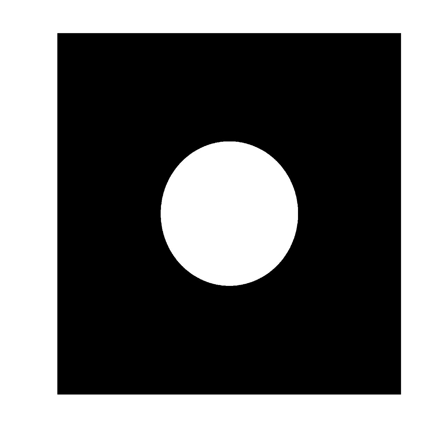
           $\Gamma_{-}(0)$ $\Gamma_{-}(1)$ $\Gamma_{-}(2)$ $\Gamma_{-}(3)$ $\Gamma_{-}(4)$        

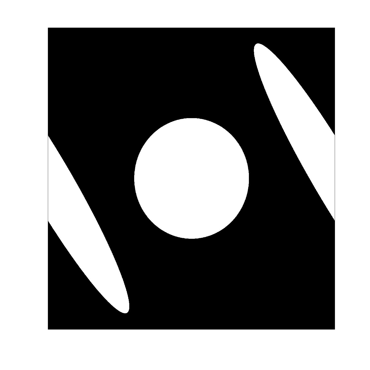
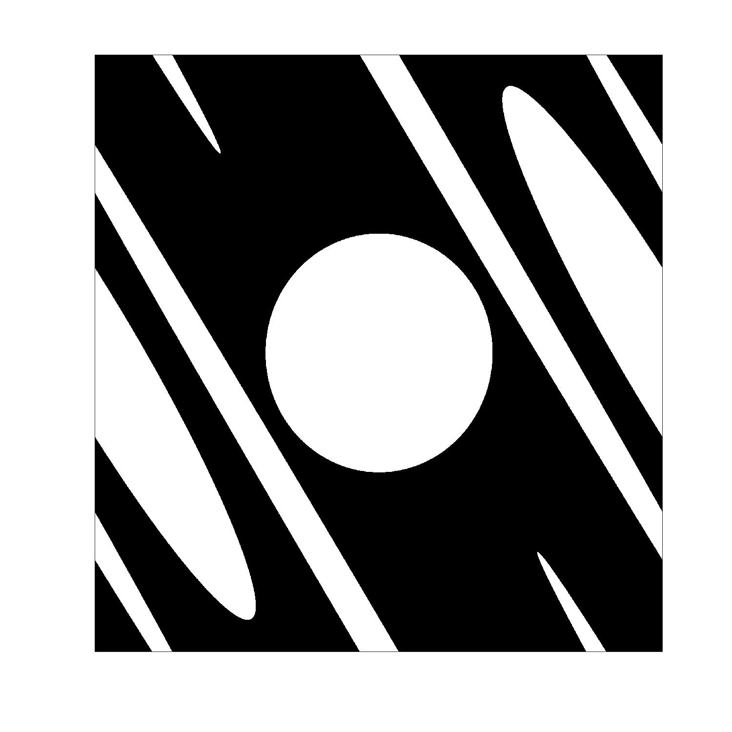
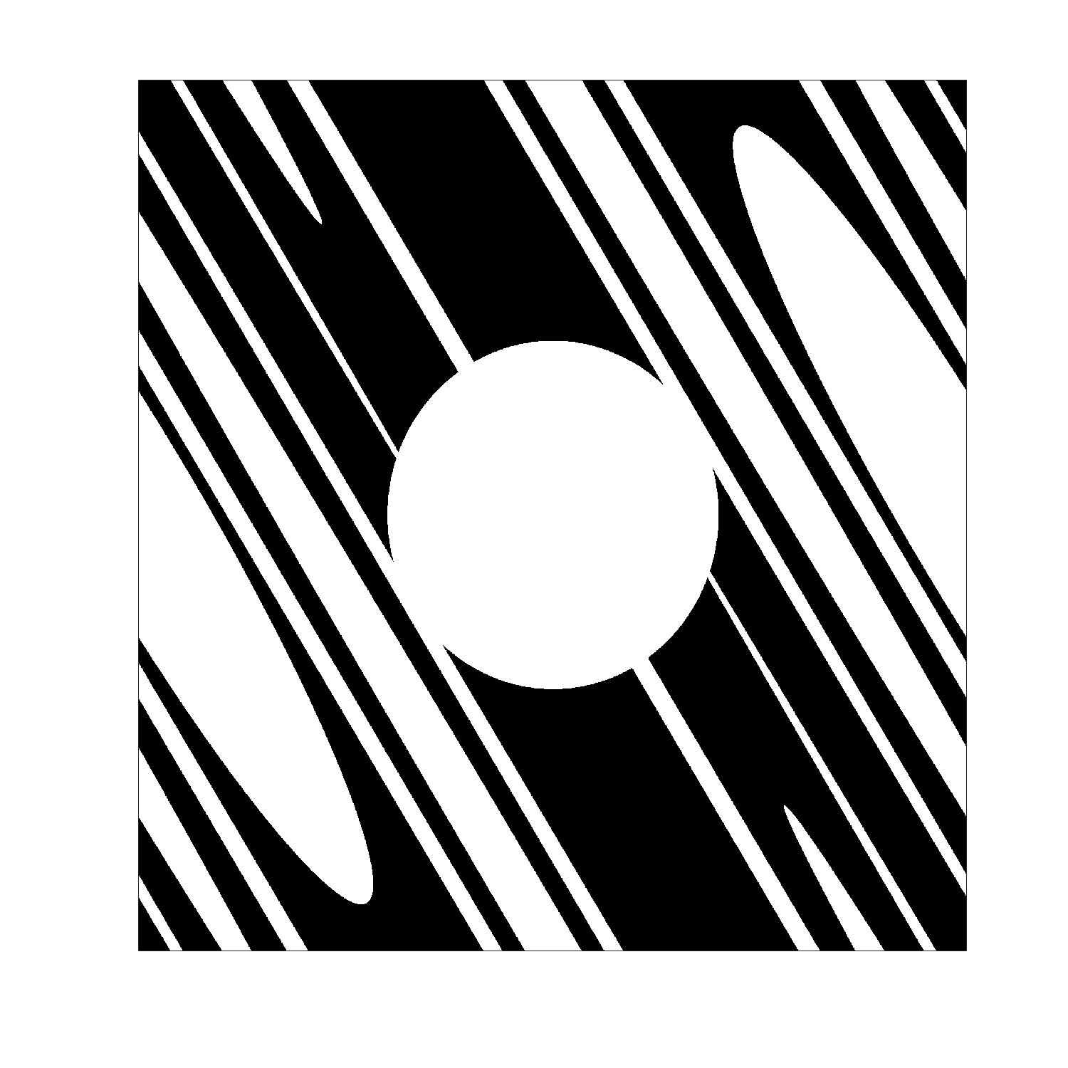
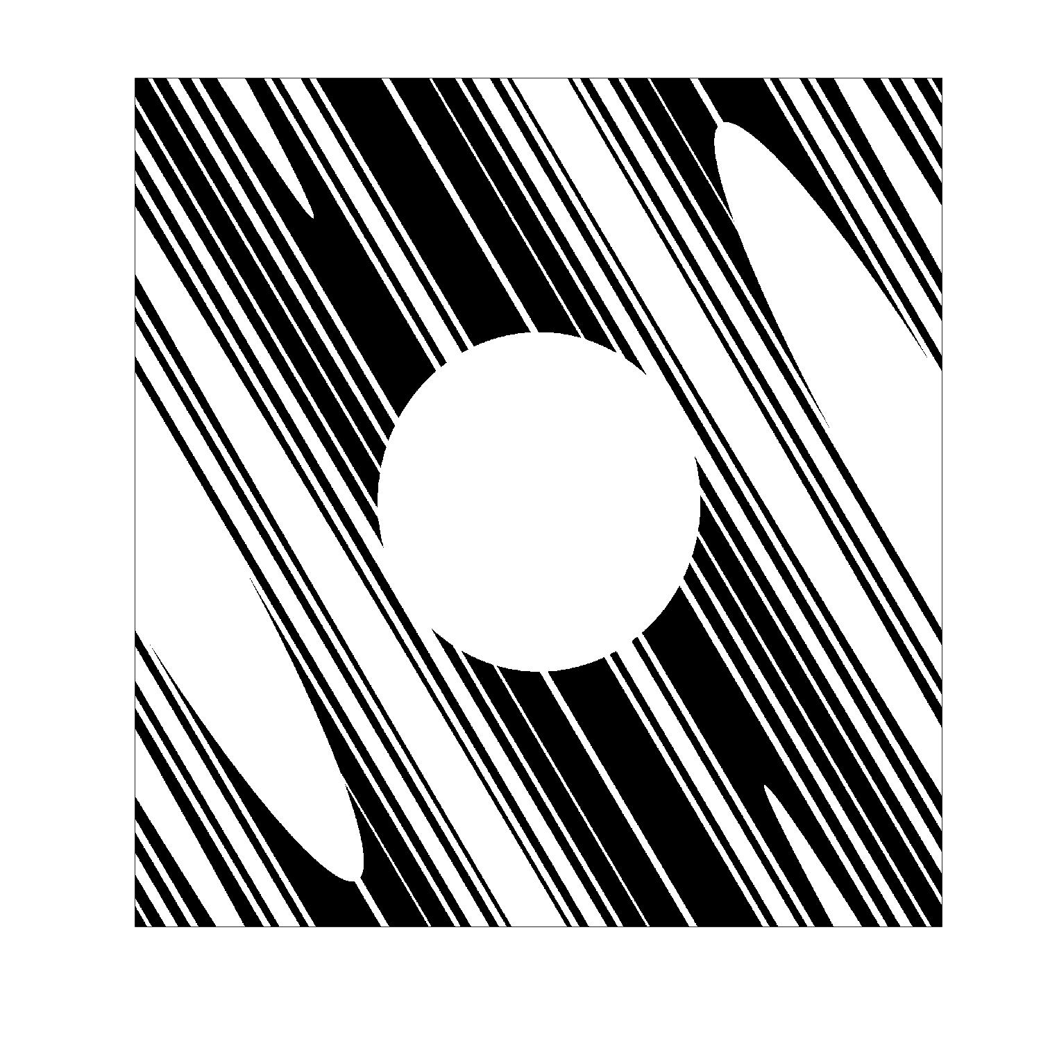
Figure 4. The sets $\Gamma_{\pm}(T)$ (in black) with the flow direction removed. This figure was produced using numerics for the closely related Arnold cat map $(x,y)\mapsto(2x+y,x+y)$ on the torus $\mathbb{R}^{2}/\mathbb{Z}^{2}$. The ‘hole’ $\pi^{-1}(\Omega)$ is the white disk pictured on the leftmost figures. We see that the sets $\Gamma_{+}(T)$ are smooth in the unstable direction $\mathbb{R}(2,\sqrt{5}-1)$. Similarly the sets $\Gamma_{-}(T)$ are smooth in the stable direction $\mathbb{R}(2,-1-\sqrt{5})$.

To obtain (3.3) from the fractal uncertainty principle we use the hyperbolicity of the geodesic flow, which gives the stable/unstable decomposition of the tangent space to $S^{*}M$ at each point into three subspaces: the space tangent to the flow, the stable space, and the unstable space. The differential of the flow contracts vectors in the stable space and expands those in the unstable space, with exponential rate $e^{t}$.

The stable/unstable decomposition implies that the set $\Gamma_{+}(T)$ is smooth along the unstable direction and the flow direction, but it is $\nu$-porous on scales $e^{-T}$ to 1 in the stable direction where porosity is understood similarly to Definition 2.7. Same is true for the set $\Gamma_{-}(T)$, with the roles of stable/unstable directions reversed – see Figure 4. The pores at scale $\alpha\in[e^{-T},1]$ come from the restriction that $\varphi_{t}(x,\xi)\notin\pi^{-1}(\Omega)$ when $\alpha\sim e^{-|t|}$, and the porosity constant $\nu$ depends on $\Omega$. Using Fourier integral operators we can deduce the norm bound (3.3) from the hyperbolic FUP for porous sets, Theorem 2.19.

The case of variable curvature considered in [DJN19] presents many additional challenges. First of all, the expansion rate of the flow is not constant, which means that the propagation time $T$ has to depend on the base point. Secondly, the stable/unstable foliations are not $C^{\infty}$, thus we cannot put the operators $A_{\pm}$ into pseudodifferential calculi defined in [DZ16], and cannot use Fourier integral operators to reduce (3.3) to an uncertainty estimate (2.17). Finally, even if we could reduce to the estimate (2.17), the corresponding phase $\Phi$ would not be $C^{\infty}$ owing again to the lack of smoothness of the stable/unstable foliations. The paper [DJN19] thus employs a different strategy to reduce (2.17) to the uncertainty principle for the Fourier transform (2.4), using $C^{1+}$ regularity of the stable/unstable foliations and a microlocal argument in place of the proof of Theorem 2.17 which was described in §2.5.

3.2. Spectral gaps

We now give an application of FUP to open quantum chaos, namely spectral gaps on noncompact hyperbolic surfaces. Assume that $(M,g)$ is a connected complete noncompact hyperbolic surface which is convex co-compact, that is its infinite ends are funnels. (See the book of Borthwick [Bo16] for an introduction to scattering on hyperbolic surfaces.) Each such surface can be realized as a quotient $M=\Gamma\backslash\mathbb{H}^{2}$ of the Poincaré upper half-plane model of the hyperbolic space

$$\mathbb{H}^{2}=\{z\in\mathbb{C}\mid\operatorname{Im}z>0\},\quad g={|dz|^{2}\over|\operatorname{Im}z|^{2}}$$

by a Schottky group $\Gamma\subset\operatorname{SL}_{2}(\mathbb{R})$ constructed in §2.4. Here each $\gamma\in\operatorname{SL}_{2}(\mathbb{R})$ defines an isometry of $(\mathbb{H}^{2},g)$ by the formula (2.11), where $x\in\dot{\mathbb{R}}$ is replaced by $z\in\mathbb{H}^{2}$. If $I_{1},\dots,I_{2r}$ are the intervals used to define the Schottky structure and $D_{w}\subset\mathbb{C}$, $w\in\{1,\dots,2r\}$, are disks with diameters $I_{w}$, then $M$ can be obtained from the fundamental domain

$$\mathcal{F}:=\mathbb{H}^{2}\setminus\bigsqcup_{w=1}^{2r}D_{w}$$ (3.4)

by gluing each half-circle $\mathbb{H}^{2}\cap\partial D_{w}$ with $\mathbb{H}^{2}\cap\partial D_{\overline{w}}$ by the map $\gamma_{w}$. See [Bo16, §15.1] for more details and Figure 5 for an example. We assumed in §2.4 that $r\geq 2$, this corresponds to $\Gamma$ being a nonelementary group; equivalently, we assume that $M$ is neither the hyperbolic space nor a hyperbolic cylinder.

Figure 5. A tessellation of the hyperbolic plane $\mathbb{H}^{2}$ (pictured here in the Poincaré disk model, with $\dot{\mathbb{R}}$ pictured as the unit circle) by fundamental domains of a convex co-compact group $\Gamma$ constructed using the procedure in §2.4 with $r=2$. The quotient $\Gamma\backslash\mathbb{H}^{2}$ is a surface with three funnel ends. The fundamental domain defined in (3.4) is shaded. The dashed line is a geodesic on $\mathbb{H}^{2}$ whose limiting starting point (denoted by the circle) does not lie in the limit set $\Lambda_{\Gamma}$ but whose limiting ending point (denoted by the triangle) lies in the limit set. The projection of this geodesic to the quotient is trapped as $t\to\infty$ but not as $t\to-\infty$.

The limit set $\Lambda_{\Gamma}\subset\mathbb{R}$, defined in (2.12), determines the structure of trapped geodesics on $M$. More precisely, we say a geodesic $\theta(t)$ on $M$ is trapped as $t\to+\infty$ if $\theta(t)$ does not go to an infinite end of $M$ as $t\to+\infty$. Similarly we define the notion of being trapped as $t\to-\infty$. We lift $\theta$ to a geodesic on $\mathbb{H}^{2}$, which is a half-circle starting at some point $\theta_{-}\in\dot{\mathbb{R}}$ and ending at some point $\theta_{+}\in\dot{\mathbb{R}}$. Then

$$\theta\text{ is trapped as }t\to\pm\infty\quad\Longleftrightarrow\quad\theta_{\pm}\in\Lambda_{\Gamma}.$$ (3.5)

See Figure 5 and [Bo16, §14.8].

We now define the ‘quantum’ objects associated to the surface $M$, called scattering resonances. These are the poles of the meromorphic continuation of the $L^{2}$ resolvent,

$$R(\lambda)=\Big{(}-\Delta_{g}-\lambda^{2}-{1\over 4}\Big{)}^{-1}:\begin{cases}L^{2}(M)\to L^{2}(M),&\operatorname{Im}\lambda>0;\\ L^{2}_{\operatorname{comp}}(M)\to L^{2}_{\operatorname{loc}}(M),&\operatorname{Im}\lambda\leq 0.\end{cases}$$

See [DZ19, Chapter 5] and [Bo16, Chapter 8] for the existence of this meromorphic continuation and an overview of hypebolic scattering, and Figure 6 for an example.

Resonances describe long time behavior of solutions to the (modified) wave equation $(\partial_{t}^{2}-\Delta_{g}-{1\over 4})v(t,x)=0$ by the following resonance expansion

$$v(t,x)\sim\sum_{\lambda_{j}\text{ resonance}}e^{-it\lambda_{j}}v_{j}(x)\quad\text{as }t\to\infty,\ x\text{ bounded}.$$ (3.6)

See [DZ19, Chapter 1] for more details and various applications of resonances.

Figure 6. Resonances for a three-funnel hyperbolic surface (similar to the one on Figure 5), plotted using data provided by David Borthwick and Tobias Weich. The topmost resonance $i(\delta-{1\over 2})$ is marked by an asterisk and the red line is $\{\operatorname{Im}z=\delta-{1\over 2}\}$. See [Bo14, BW16], and [Bo16, Chapter 16] for more pictures of resonances of hyperbolic surfaces. As explained in these works, numerically estimating the size of the essential spectral gap is very challenging.

The main topic of this section is the concept of an essential spectral gap:

Definition 3.4.

We say that $M$ has an essential spectral gap of size $\beta$, if the half-plane $\{\operatorname{Im}\lambda\geq-\beta\}$ only has finitely many resonances. (Such a gap is nontrivial only for $\beta>0$.)

In the expansion (3.6), the real part of a resonance $\lambda_{j}$ gives the rate of oscillation of the function $e^{-it\lambda_{j}}$, and the (negative) imaginary part gives the rate of decay. Thus an essential spectral gap of size $\beta>0$ implies exponential decay $\mathcal{O}(e^{-\beta t})$ of solutions to the wave equation, modulo a finite dimensional space corresponding to resonances with $\operatorname{Im}\lambda_{j}\geq-\beta$.

We emphasize that resonances can be defined for a variety of quantum open systems (for instance, obstacle scattering or wave equations on black holes) and having an essential spectral gap is equivalent to exponential local energy decay of high frequency waves, see for instance [DZ19, Theorems 2.9 and 5.40]. This in particular has applications to nonlinear equations, such as black hole stability (see Hintz–Vasy [HV18]) and Strichartz estimates (see Burq–Guillarmou–Hassell [BGH10] and Wang [Wa17]).

Existence of an essential spectral gap depends on the structure of trapped classical trajectories (see [DZ19, Chapter 6]). For a convex co-compact hyperbolic surface, the set of all trapped geodesics has fractal structure (by (3.5)) and the geodesic flow has hyperbolic behavior on this set (namely it has a stable/unstable decomposition). Thus convex co-compact hyperbolic surfaces serve as a model for more general systems with fractal hyperbolic trapped sets. The latter class includes scattering by several convex obstacles (see Figure 7), where spectral gaps have been observed in microwave scattering experiments by Barkhofen et al. [B^∗13]. We refer to the reviews of Nonnenmacher [No11] and Zworski [Zw17] for an overview of results on spectral gaps for open quantum chaotic systems.

Figure 7. A ‘real-world’ example of a system with fractal hyperbolic trapping: the billiard ball map on the exterior of three disks in $\mathbb{R}^{2}$. The trapped billiard trajectories are shown on the left. On the right is the set of trajectories trapped backward (top) and forward (bottom) restricted to the boundary of one disk, where the horizontal variable is the point on the boundary and the vertical variable is the angle of the tangent vector to the boundary. (See [Dy18, §5.2] for details.) The fractal uncertainty principle in this setting would say that no function can be localized in the position-frequency space to both forward and backward trapped sets.

Coming back to hyperbolic surfaces, it is well-known that there is an essential spectral gap of size $\beta=0$. In fact, resonances with $\operatorname{Im}\lambda>0$ correspond to the (finitely many) $L^{2}$ eigenvalues of $-\Delta_{g}$ in $[0,{1\over 4})$. There is also the Patterson–Sullivan gap $\beta={1\over 2}-\delta$ (see [Pa76, Su79]) where $\delta\in(0,1)$ is the dimension of the limit set (see §2.4). In fact, the resonance with the largest imaginary part is given by $\lambda=i(\delta-{1\over 2})$, see [Bo16, Theorem 14.15]. Thus we have an essential spectral gap of the size $\beta=\max(0,{1\over 2}-\delta)$.

The application of FUP to spectral gaps is based on the following

Theorem 3.5.

[DZ16, DZ17] Let $M=\Gamma\backslash\mathbb{H}^{2}$ be a convex co-compact hyperbolic surface and $\Lambda_{\Gamma}\subset\mathbb{R}$ be the limit set of the group $\Gamma$. Denote by $\Lambda_{\Gamma}(h)$ the $h$-neighborhood of $\Lambda_{\Gamma}$.

Assume that $X=Y=\Lambda_{\Gamma}(h)$ satisfies the hyperbolic uncertainty principle (2.17) with some exponent $\beta>0$, for the phase function $\Phi(x,y)=\log|x-y|$ from (2.15) and every choice of the amplitude $b\in C^{\infty}_{\mathrm{c}}(\mathbb{R}^{2}\setminus\{x=y\})$. Then $M$ has an essential spectral gap of size $\beta-\varepsilon$ for each $\varepsilon>0$.

Two different proofs of Theorem 3.5 are given in [DZ16] and [DZ17]. The proof in [DZ16] uses microlocal methods similar to the proof of Theorem 3.1. Roughly speaking, if $\lambda$ is a resonance with $|\operatorname{Re}\lambda|=h^{-1}\gg 1$ and $\operatorname{Im}\lambda=-\nu$, then there exists a resonant state which is a solution $u$ to the equation $(-\Delta_{g}-\lambda^{2}-{1\over 4})u=0$ satisfying a certain outgoing condition at the infinite ends of $M$. Next, $u$ is microlocalized $h$-close to the set of backward trapped trajectories, and it has mass at least $h^{2\nu}$ on the $h$-neighborhood of the set of forward trapped trajectories (here mass is the square of the $L^{2}$ norm). The fractal uncertainty principle then implies that $h^{\nu}\leq h^{\beta}$, that is $\nu\geq\beta$. Here the limit set enters via the description of trapped trajectories in (3.5). Compared to the compact setting described in §3.1 a key additional ingredient is the work of Vasy [Va13a, Va13b] on effective meromorphic continuation of the scattering resolvent.

The other proof of Theorem 3.5, given in [DZ17], proceeds by bounding the spectral radius of the transfer operator of the Bowen–Series map. That proof is much shorter than [DZ16] but the method is less likely to be applicable to more general open hyperbolic systems.

Combining Theorem 3.5 with the fractal uncertainty principle from Theorems 2.17–2.18 we obtain

Theorem 3.6.

Let $M,\Lambda_{\Gamma}$ be as in Theorem 3.5 and $\delta\in(0,1)$ be the dimension of $\Lambda_{\Gamma}$. Then $M$ has an essential spectral gap of size $\beta$ for some $\beta>\max(0,{1\over 2}-\delta)$. See Figure 8.

Figure 8. Numerically computed essential spectral gaps $\beta$ for symmetric 3-funneled and 4-funneled surfaces from [BW16, Figure 14] (specifically, $G_{100}^{I_{1}}$ in the notation of [BW16]). Each point corresponds to one surface and has coordinates $(\delta,\beta)$. The solid line is the standard gap $\beta=\max(0,{1\over 2}-\delta)$. The dashed line is the Jakobson–Naud conjecture $\beta={1-\delta\over 2}$.

An essential spectral gap of size $\beta>{1\over 2}-\delta$ when $0<\delta\leq{1\over 2}$ was previously established by Naud [Na05]. This improvement over the Patterson–Sullivan gap was used to get an asymptotic formula for the number $\mathcal{N}(L)$ of primitive closed geodesics of period $\leq L$ of the form

$$\mathcal{N}(L)=\operatorname{li}(e^{\delta T})+\mathcal{O}(e^{(\delta-\varepsilon)T}),\quad\operatorname{li}(x):=\int_{2}^{x}{dt\over\log t}$$

for some $\varepsilon>0$, see [Na05, Theorem 1.4]. Spectral gaps with $\beta>{1\over 2}-\delta$ also have important applications to diophantine problems in number theory, see Bourgain–Gamburd–Sarnak [BGS11], Magee–Oh–Winter [MOW16], and the review of Sarnak [Sa13]. A spectral gap $\beta>{1\over 2}-\delta$ depending only on the dimension $\delta$ of the limit set is given in Theorem 5.3 below.

Jakobson–Naud [JN10] conjectured an essential spectral gap of size $\beta={1-\delta\over 2}$, see Figure 8. This conjecture corresponds to the upper limit of possible results that could be proved using FUP: indeed, by applying $\operatorname{1\hskip-2.75ptl}_{\Lambda_{\Gamma}(h)}\mathcal{B}_{h}\operatorname{1\hskip-2.75ptl}_{\Lambda_{\Gamma}(h)}$ to a function localized in an $h$-sized interval inside $\Lambda_{\Gamma}(h)$ and using that $\operatorname{vol}(\Lambda_{\Gamma}(h))\sim h^{1-\delta}$ we see that if (2.17) holds with some value of $\beta$, then we necessarily have $\beta\leq{1-\delta\over 2}$. While the Jakobson–Naud conjecture is out of reach of current methods, its analogue is known to hold in certain special cases in the ‘toy model’ setting of open quantum cat maps, see [DJ17, §3.5].

For more general open systems with hyperbolic trapping, an essential spectral gap was known under a pressure condition which generalizes the inequality $\delta<{1\over 2}$, by Ikawa [Ik88], Gaspard–Rice [GR89], and Nonnenmacher–Zworski [NZ09]. In some cases there exists a gap strictly larger than the pressure gap: see Petkov–Stoyanov [PS10] and Stoyanov [St11, St12], in addition to the work of Naud mentioned above.

In contrast with the pressure gap and improvements over it, Theorem 3.6 gives an essential spectral gap $\beta>0$ for all convex co-compact hyperbolic surfaces. This makes it a special case of the conjecture of Zworski [Zw17, §3.2, Conjecture 3] that every open hyperbolic system has an essential spectral gap.

4. FUP for discrete Cantor sets

We now discuss FUP for a special class of regular fractal sets, namely discrete Cantor sets. In this setting we provide a complete proof of the fractal uncertainty principle of Theorems 2.12–2.13. In [DJ17] this special case of FUP was applied to obtain an essential spectral gap for the ‘toy model’ of quantum open baker’s maps, similarly to the application to convex co-compact hyperbolic surfaces discussed in §3.2. We refer to [DJ17] for a discussion of these quantum maps and more qualitative information on FUP for Cantor sets.

A discrete Cantor set is a subset of $\mathbb{Z}_{N}:=\{0,\dots,N-1\}$ of the form

$$\mathcal{C}_{k}:=\big{\{}a_{0}+a_{1}M+\cdots+a_{k-1}M^{k-1}\mid a_{0},\dots,a_{k-1}\in\mathcal{A}\big{\}},\quad N:=M^{k}$$ (4.1)

where $k$ (called the order of the set) is a large natural number and we fixed

• an integer $M\geq 3$, called the base, and

• a nonempty subset $\mathcal{A}\subset\{0,\dots,M-1\}$, called the alphabet.

In other words, $\mathcal{C}_{k}$ is the set of numbers of length $k$ in base $M$ with all digits in $\mathcal{A}$. Note that $|\mathcal{C}_{k}|=|\mathcal{A}|^{k}=N^{\delta}$ where the dimension $\delta$ is defined by

$$\delta:={\log|\mathcal{A}|\over\log M}\in[0,1].$$ (4.2)

We have $0<\delta<1$ except in the trivial cases $|\mathcal{A}|=1$ and $|\mathcal{A}|=M$. The number $\delta$ is the dimension of the limiting Cantor set

$$\mathcal{C}_{\infty}:=\bigcap_{k\geq 1}\bigcup_{j\in\mathcal{C}_{k}}\Big{[}{j\over M^{k}},{j+1\over M^{k}}\Big{]}\subset[0,1].$$ (4.3)

More precisely, $\mathcal{C}_{\infty}$ is $\delta$-regular on scales 0 to 1 similarly to Example 2.6, see [DJ18a, Lemma 5.4] for more details. The middle third Cantor set corresponds to $M=3$, $\mathcal{A}=\{0,2\}$.

The main result of this section is the following discrete version of FUP:

Theorem 4.1.

Let $\mathcal{C}_{k}\subset\mathbb{Z}_{N}$, $N=M^{k}$, be the Cantor set from (4.1) for some choice of $M,\mathcal{A}$. Define the unitary discrete Fourier transform

$$\mathcal{F}_{N}:\mathbb{C}^{N}\to\mathbb{C}^{N},\quad\mathcal{F}_{N}u(j)={1\over\sqrt{N}}\sum_{\ell=0}^{N-1}\exp\Big{(}-{2\pi ij\ell\over N}\Big{)}u(\ell).$$ (4.4)

Let $\delta$ be defined in (4.2) and assume that $0<\delta<1$. Then there exist constants

$$\beta>\max\Big{(}0,{1\over 2}-\delta\Big{)}$$ (4.5)

and $C$, both depending only on $M,\mathcal{A}$, such that the set $\mathcal{C}_{k}$ satisfies the discrete uncertainty principle

$$\|\operatorname{1\hskip-2.75ptl}_{\mathcal{C}_{k}}\mathcal{F}_{N}\operatorname{1\hskip-2.75ptl}_{\mathcal{C}_{k}}\|_{\mathbb{C}^{N}\to\mathbb{C}^{N}}\leq CN^{-\beta}.$$ (4.6)

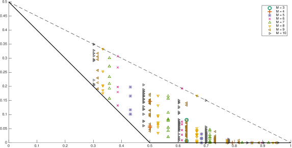
Figure 9. Numerically approximated fractal uncertainty exponents for all possible alphabets with $M\leq 10$ and $0<\delta<1$. Here the horizontal axis represents $\delta$ and the vertical axis represents $\beta$. The solid black line is $\beta=\max(0,{1\over 2}-\delta)$ and the dashed line is $\beta={1-\delta\over 2}$. See [DJ17, Figure 3] for details.

Remark 4.2.

The discrete uncertainty principle (4.6) is related to the continuous uncertainty principle (2.4) for $X=Y=\mathcal{C}_{\infty}+[0,h]$ and $h=(2\pi N)^{-1}$, see [DJ18a, Proposition 5.8].

Remark 4.3.

It is easy to see that (4.6) holds with $C=1$ and $\beta=\max(0,{1\over 2}-\delta)$. Indeed, since $\mathcal{F}_{N}$ is unitary, the left-hand side of (4.6) is bounded above by 1. On the other hand, denoting by $\|\bullet\|_{\operatorname{HS}}$ the Hilbert–Schmidt norm, we have

$$\|\operatorname{1\hskip-2.75ptl}_{\mathcal{C}_{k}}\mathcal{F}_{N}\operatorname{1\hskip-2.75ptl}_{\mathcal{C}_{k}}\|_{\mathbb{C}^{N}\to\mathbb{C}^{N}}\leq\|\operatorname{1\hskip-2.75ptl}_{\mathcal{C}_{k}}\mathcal{F}_{N}\operatorname{1\hskip-2.75ptl}_{\mathcal{C}_{k}}\|_{\operatorname{HS}}=N^{\delta-1/2}.$$ (4.7)

A natural question to ask is the dependence of the largest exponent $\beta$ for which (4.6) holds on the alphabet $\mathcal{A}$. This dependence can be quite complicated, see Figure 9. There exist various lower and upper bounds on $\beta$ depending on $M,\delta$, see [DJ17, §3]. In particular, for each $\delta\in(0,{1\over 2}]$ the improvement in (4.5) may be arbitrarily small, namely there exists a sequence $(M_{j},\mathcal{A}_{j})$ such that the corresponding dimensions $\delta_{j}$ converge to $\delta$ and the FUP exponents $\beta_{j}$ converge to ${1\over 2}-\delta$ – see [DJ17, Proposition 3.17]. For $\delta>{1\over 2}$ numerics suggest that $\beta$ could be exponentially small in $M$, supporting the following

Conjecture 4.4.

Fix $\delta\in(1/2,1)$. Then there exists a sequence of pairs $(M_{j},\mathcal{A}_{j})$ such that

$$\delta(M_{j},\mathcal{A}_{j})\to\delta,\quad\beta(M_{j},\mathcal{A}_{j})\to 0.$$

Here $\delta(M,\mathcal{A})=\log_{M}|\mathcal{A}|$ and

$$\beta(M,\mathcal{A}):=-\limsup_{k\to\infty}{\log\|\operatorname{1\hskip-2.75ptl}_{\mathcal{C}_{k}}\mathcal{F}_{N}\operatorname{1\hskip-2.75ptl}_{\mathcal{C}_{k}}\|_{\mathbb{C}^{N}\to\mathbb{C}^{N}}\over\log N},\quad N:=M^{k}.$$

As follows from the above discussion and illustrated by Figure 9, we expect that $\beta-\max(0,{1\over 2}-\delta)$ may be very small for some choice of $M,\mathcal{A}$. However, the following conjecture states that if we dilate one of the sets $\mathcal{C}_{k}$ by a generic factor, then FUP holds with a larger value of $\beta$, depending only on the dimension $\delta$:

Conjecture 4.5.

Fix $M,\mathcal{A}$ with $0<\delta<1$, take $\alpha\in[1,M]$, and consider the dilated Fourier transform

$$\mathcal{F}_{N,\alpha}:\mathbb{C}^{N}\to\mathbb{C}^{N},\quad\mathcal{F}_{N,\alpha}u(j)={1\over\sqrt{N}}\sum_{\ell=0}^{N-1}\exp\Big{(}-{2\pi i\alpha j\ell\over N}\Big{)}u(\ell).$$ (4.8)

Show that there exists $\beta>\max(0,{1\over 2}-\delta)$ depending only on $\delta$ such that for a generic choice of $\alpha\in[1,M]$ we have as $k\to\infty$

$$\|\operatorname{1\hskip-2.75ptl}_{\mathcal{C}_{k}}\mathcal{F}_{N,\alpha}\operatorname{1\hskip-2.75ptl}_{\mathcal{C}_{k}}\|_{\mathbb{C}^{N}\to\mathbb{C}^{N}}=\mathcal{O}(N^{-\beta}),\quad N:=M^{k}.$$ (4.9)

We note that existence of $\beta$ depending on $M,\mathcal{A}$ follows from the general FUP in Theorems 2.12–2.13. Note also that while we do not in general have $\|\mathcal{F}_{N,\alpha}\|\leq 1$, by applying Schur’s Lemma to the matrix $\mathcal{F}_{N,\alpha}^{*}\mathcal{F}_{N,\alpha}$ we see that $\|\mathcal{F}_{N,\alpha}\|\leq C\sqrt{\log N}$.

If true (with a sufficiently good understanding of what it means for $\alpha$ to be generic), Conjecture 4.5 is likely to give a spectral gap depending only on $\delta$ for an open quantum baker’s map with generic size of the matrix. We refer the reader to [DJ18a, §5] for details. More precisely, if the size of the open quantum baker’s map matrix is given by $\alpha M^{k}$ where $1\leq\alpha\leq M$, then the left-hand side of [DJ18a, (5.8)] is the norm of the matrix

$$\bigg{(}{1\over\sqrt{\alpha M^{k}}}\exp\Big{(}-{2\pi ib_{j}b_{\ell}\over\alpha M^{k}}\Big{)}\bigg{)}_{j,\ell\in\mathcal{C}_{k}}$$ (4.10)

where $b_{j}$ is an integer chosen arbitrarily in the interval $\big{[}\alpha j,\alpha(j+1)\big{)}$. If we forget about the requirement that $b_{j}$ be an integer, then we may take $b_{j}:=\alpha j$, in which case the matrix (4.10) has entries $\big{(}{1\over\sqrt{\alpha M^{k}}}e^{-2\pi i\alpha j\ell/M^{k}}\big{)}_{j,\ell\in\mathcal{C}_{k}}$, and its norm equals the left-hand side of (4.9) up to the constant factor $\sqrt{\alpha}$.

One possible approach to Conjecture 4.5 would be to use the following corollary of Schur’s Lemma (see the proof of [DJ17, Lemma 3.8])

$$\begin{gathered}\|\operatorname{1\hskip-2.75ptl}_{\mathcal{C}_{k}}\mathcal{F}_{N,\alpha}\operatorname{1\hskip-2.75ptl}_{\mathcal{C}_{k}}\|_{\mathbb{C}^{N}\to\mathbb{C}^{N}}\leq\tilde{r}_{k,\alpha}\quad\text{where}\\ \tilde{r}_{k,\alpha}^{2}=\max_{j\in\mathcal{C}_{k}}\sum_{\ell\in\mathcal{C}_{k}}|F_{k,\alpha}(j-\ell)|,\quad F_{k,\alpha}(j)={1\over N}\sum_{r\in\mathcal{C}_{k}}\exp\Big{(}-{2\pi i\alpha rj\over N}\Big{)}.\end{gathered}$$ (4.11)

For numerical evidence in support of Conjecture 4.5, see Figures 10–11.

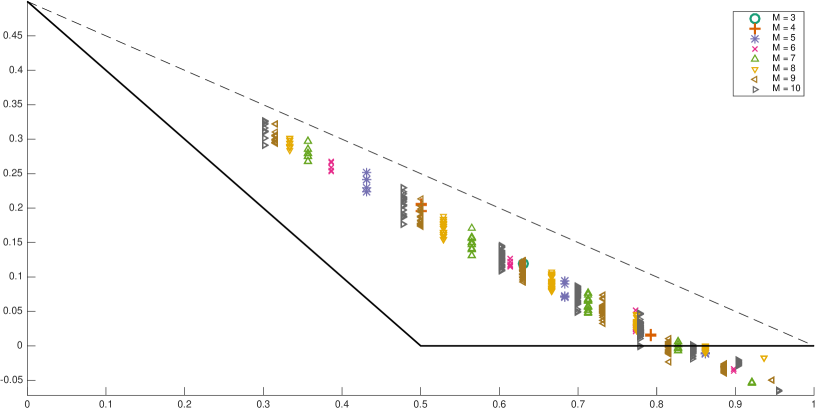
Figure 10. Numerically approximated fractal uncertainty exponents for all possible alphabets with $M\leq 10$ and $0<\delta<1$, using the dilated Fourier transform $\mathcal{F}_{N,\alpha}$ from (4.8) in place of $\mathcal{F}_{N}$, with $\alpha:=(1+\sqrt{5})/2$, taking $k$ large and assuming constant $1$ in the $\mathcal{O}(\bullet)$ in (4.9). We see that the worst FUP exponents are generally larger than those on Figure 9, supporting Conjecture 4.5. This data has to be interpreted with more caution than the one on Figure 9. In particular, some points have $\beta<0$, because the operator $\mathcal{F}_{N,\alpha}$ no longer has norm bounded by 1.

Figure 11. Graphs of the quantities $\beta_{k,\alpha}:=-\log\tilde{r}_{k,\alpha}/\log N$ as functions of $\alpha$ for two values of $k$ where $\tilde{r}_{k,\alpha}$ is defined in (4.11). The parameters of the Cantor set are $M=4$, $\mathcal{A}=\{0,1\}$, and in this case $|F_{k,\alpha}(j)|=2^{-k}\prod_{q=1}^{k}|\cos(4^{-q}\pi\alpha j)|$. We note the dips at $\alpha=1,3,4$, with $\beta_{k,\alpha}$ being much larger for generic $\alpha$ than at the dips. For $\alpha=2$ we have $\beta_{k,\alpha}={1\over 4}$ due to the choice of the alphabet, this is similar to the special alphabets considered in [DJ17, §3.5].

4.1. Proof of discrete FUP

We now give a proof of Theorem 4.1, following [DJ17, §3]. Compared to the general case the proof is greatly simplified by the following submultiplicative property which uses the special structure of Cantor sets:

Lemma 4.6.

Put

$$r_{k}:=\|\operatorname{1\hskip-2.75ptl}_{\mathcal{C}_{k}}\mathcal{F}_{N}\operatorname{1\hskip-2.75ptl}_{\mathcal{C}_{k}}\|_{\mathbb{C}^{N}\to\mathbb{C}^{N}},\quad N:=M^{k}.$$

Then for all $k_{1},k_{2}$ we have

$$r_{k_{1}+k_{2}}\leq r_{k_{1}}\cdot r_{k_{2}}.$$

Proof.

Denote

$$k:=k_{1}+k_{2},\quad N_{j}:=M^{k_{j}},\quad N:=M^{k}.$$

We define the space

$$\ell^{2}(\mathcal{C}_{k})=\{u\in\mathbb{C}^{N}\mid\operatorname{supp}u\subset\mathcal{C}_{k}\}.$$

Then $r_{k}$ is the norm of the operator

$$\mathcal{G}_{k}:\ell^{2}(\mathcal{C}_{k})\to\ell^{2}(\mathcal{C}_{k}),\quad\mathcal{G}_{k}u=\operatorname{1\hskip-2.75ptl}_{\mathcal{C}_{k}}\mathcal{F}_{N}u.$$

We will write $\mathcal{G}_{k}$ in terms of $\mathcal{G}_{k_{1}},\mathcal{G}_{k_{2}}$ using a procedure similar to the one used in the Fast Fourier Transform (FFT) algorithm. Take

$$u\in\ell^{2}(\mathcal{C}_{k}),\quad v:=\mathcal{G}_{k}u.$$

We associate to $u,v$ the $|\mathcal{A}|^{k_{1}}\times|\mathcal{A}|^{k_{2}}$ matrices $U,V$ defined as follows:

$$U_{ab} =u(N_{1}\cdot b+a)$$

$$V_{ab} =v(N_{2}\cdot a+b)$$

for all $a\in\mathcal{C}_{k_{1}}$ and $b\in\mathcal{C}_{k_{2}}$. Here we use the fact that

$$\mathcal{C}_{k}=N_{2}\cdot\mathcal{C}_{k_{1}}+\mathcal{C}_{k_{2}}=N_{1}\cdot\mathcal{C}_{k_{2}}+\mathcal{C}_{k_{1}}.$$

Note that the norms of $u,v$ are equal to the Hilbert–Schmidt norms of $U,V$:

$$\|u\|^{2}=\sum_{a,b}|U_{ab}|^{2},\quad\|v\|^{2}=\sum_{a,b}|V_{ab}|^{2}.$$

We now write the identity $v=\mathcal{G}_{k}u$ in terms of the matrices $U,V$:

$$V_{ab}={1\over\sqrt{N}}\sum_{p\in\mathcal{C}_{k_{1}}\atop q\in\mathcal{C}_{k_{2}}}\exp\Big{(}-{2\pi i(N_{2}\cdot a+b)(N_{1}\cdot q+p)\over N}\Big{)}U_{pq}.$$

Here is where a small miracle happens: the product of $N_{2}\cdot a$ and $N_{1}\cdot q$ is divisible by $N$, so it can be removed from the exponential. That is,

$$V_{ab}={1\over\sqrt{N}}\sum_{p,q}\exp\Big{(}-{2\pi iap\over N_{1}}\Big{)}\exp\Big{(}-{2\pi ibp\over N}\Big{)}\exp\Big{(}-{2\pi ibq\over N_{2}}\Big{)}U_{pq}.$$

It follows that the matrix $V$ can be obtained from $U$ in the following three steps:

1. Replace each row of $U$ by its Fourier transform $\mathcal{G}_{k_{2}}$, obtaining the matrix

   $$U^{\prime}_{pb}={1\over\sqrt{N_{2}}}\sum_{q\in\mathcal{C}_{k_{2}}}\exp\Big{(}-{2\pi ibq\over N_{2}}\Big{)}U_{pq}.$$

2. Multiply the entries of $U^{\prime}$ by twist factors, obtaining the matrix

   $$V^{\prime}_{pb}=\exp\Big{(}-{2\pi ibp\over N}\Big{)}U^{\prime}_{pb}.$$

3. Replace each column of $V^{\prime}$ by its Fourier transform $\mathcal{G}_{k_{1}}$, obtaining the matrix

   $$V_{ab}={1\over\sqrt{N_{1}}}\sum_{p\in\mathcal{C}_{k_{1}}}\exp\Big{(}-{2\pi iap\over N_{1}}\Big{)}V^{\prime}_{pb}.$$

Now, we have

$$\|U^{\prime}\|_{\operatorname{HS}}\leq r_{k_{2}}\|U\|_{\operatorname{HS}},\quad\|V^{\prime}\|_{\operatorname{HS}}=\|U^{\prime}\|_{\operatorname{HS}},\quad\|V\|_{\operatorname{HS}}\leq r_{k_{1}}\|V^{\prime}\|_{\operatorname{HS}},$$

giving

$$\|v\|\leq r_{k_{1}}\cdot r_{k_{2}}\cdot\|u\|$$

which finishes the proof. ∎

Given Lemma 4.6, we see by Fekete’s Lemma that

$$\lim_{k\to\infty}{\log r_{k}\over k\log M}=\inf_{k\geq 1}{\log r_{k}\over k\log M}.$$ (4.12)

Thus to prove Theorem 4.1 it suffices to obtain the strict inequality

$$r_{k}:=\|\operatorname{1\hskip-2.75ptl}_{\mathcal{C}_{k}}\mathcal{F}_{N}\operatorname{1\hskip-2.75ptl}_{\mathcal{C}_{k}}\|_{\mathbb{C}^{N}\to\mathbb{C}^{N}}<\min(1,N^{\delta-1/2})$$ (4.13)

for just one value of $k$.

The inequality (4.13) consists of two parts, proved below:

Lemma 4.7.

There exists $k$ such that $r_{k}<1$.

Proof.

Since $\mathcal{F}_{N}$ is unitary we have $r_{k}\leq 1$. We argue by contradiction. Assume that $r_{k}=1$. Then there exists

$$u\in\mathbb{C}^{N}\setminus\{0\},\quad\|\operatorname{1\hskip-2.75ptl}_{\mathcal{C}_{k}}\mathcal{F}_{N}\operatorname{1\hskip-2.75ptl}_{\mathcal{C}_{k}}u\|=\|u\|.$$

This implies that

$$\operatorname{supp}u \subset\mathcal{C}_{k},$$ (4.14)

$$\operatorname{supp}(\mathcal{F}_{N}u) \subset\mathcal{C}_{k}.$$ (4.15)

We now use the fact that discrete Fourier transform evaluates polynomials at roots of unity. Define the polynomial

$$p(z):=\sum_{\ell=0}^{N-1}u(\ell)z^{\ell}.$$

Then

$$\mathcal{F}_{N}u(j)={1\over\sqrt{N}}\,p(e^{-2\pi ij/N}).$$

By (4.15) for each $j\in\mathbb{Z}_{N}\setminus\mathcal{C}_{k}$ we have $\mathcal{F}_{N}u(j)=0$. It follows that the number of roots of $p$ is bounded below by (here we use that $\delta<1$)

$$N-|\mathcal{C}_{k}|\geq M^{k}-(M-1)^{k}.$$

On the other hand, the set $\mathbb{Z}_{N}\setminus\mathcal{C}_{k}$ contains $M^{k-1}$ consecutive numbers (specifically $aM^{k-1},\dots,(a+1)M^{k-1}-1$ where $a\in\mathbb{Z}_{M}\setminus\mathcal{A}$; this corresponds to porosity). We shift $\mathcal{C}_{k}$ circularly (which does not change the norm $r_{k}$) to map these numbers to $(M-1)M^{k-1},\dots,M^{k}-1$. Then the degree of $p$ is smaller than $(M-1)M^{k-1}$.

Now, for $k$ large enough we have

$$M^{k}-(M-1)^{k}\geq(M-1)M^{k-1}.$$

Then the number of roots of $p$ is larger than its degree, giving a contradiction. ∎

Lemma 4.8.

For $k\geq 2$ we have $r_{k}<N^{\delta-1/2}$.

Proof.

Recall from (4.7) that $N^{\delta-1/2}$ is the Hilbert–Schmidt norm of $\operatorname{1\hskip-2.75ptl}_{\mathcal{C}_{k}}\mathcal{F}_{N}\operatorname{1\hskip-2.75ptl}_{\mathcal{C}_{k}}$, while $r_{k}$ is its operator norm. We again argue by contradiction, assuming that $r_{k}=N^{\delta-1/2}$. Then $\operatorname{1\hskip-2.75ptl}_{\mathcal{C}_{k}}\mathcal{F}_{N}\operatorname{1\hskip-2.75ptl}_{\mathcal{C}_{k}}$ is a rank 1 operator; indeed, the sum of the squares of its singular values is equal to the square of the maximal singular value. It follows that each rank 2 minor of $\operatorname{1\hskip-2.75ptl}_{\mathcal{C}_{k}}\mathcal{F}_{N}\operatorname{1\hskip-2.75ptl}_{\mathcal{C}_{k}}$ is equal to zero, namely

$$\det\begin{pmatrix}e^{-2\pi ij\ell/N}&e^{-2\pi ij\ell^{\prime}/N}\\ e^{-2\pi ij^{\prime}\ell/N}&e^{-2\pi ij^{\prime}\ell^{\prime}/N}\end{pmatrix}=0\quad\text{for all }j,j^{\prime},\ell,\ell^{\prime}\in\mathcal{C}_{k}.$$

Computing the determinant we see that

$$(j-j^{\prime})(\ell-\ell^{\prime})\in N\mathbb{Z}\quad\text{for all }j,j^{\prime},\ell,\ell^{\prime}\in\mathcal{C}_{k}.$$

However, if $k\geq 2$ we may take $j=\ell,j^{\prime}=\ell^{\prime}\in\mathcal{C}_{k}$ such that (here we use that $\delta>0$)

$$0<|j-j^{\prime}|<M\leq\sqrt{N},$$

giving a contradiction. ∎

5. Relation to Fourier decay and additive energy

We now explain how a fractal uncertainty principle can be proved if we have a Fourier decay bound or an additive energy bound on one of the sets $X,Y$. While this does not give new results (compared to Theorems 2.12–2.13) in the general setting, it leads to improvements in special cases.

Let $X,Y\subset[0,1]$ be two $h$-dependent closed sets which are $\delta$-regular on scales $h$ to 1 with some $h$-independent regularity constant $C_{R}$ (see Definition 2.2). In particular by (2.6) we have

$$\operatorname{vol}(X),\operatorname{vol}(Y)\leq Ch^{1-\delta}.$$ (5.1)

To estimate the norm on the left-hand side of the uncertainty principle (2.4), we use the $T^{*}T$ argument:

$$\|\operatorname{1\hskip-2.75ptl}_{X}\mathcal{F}_{h}\operatorname{1\hskip-2.75ptl}_{Y}\|_{L^{2}\to L^{2}}^{2}=\|\operatorname{1\hskip-2.75ptl}_{Y}\mathcal{F}_{h}^{*}\operatorname{1\hskip-2.75ptl}_{X}\mathcal{F}_{h}\operatorname{1\hskip-2.75ptl}_{Y}\|_{L^{2}\to L^{2}}.$$

We write $\mathcal{F}_{h}^{*}\operatorname{1\hskip-2.75ptl}_{X}\mathcal{F}_{h}$ as an integral operator:

$$\mathcal{F}_{h}^{*}\operatorname{1\hskip-2.75ptl}_{X}\mathcal{F}_{h}f(y)=\int_{\mathbb{R}}\mathcal{K}_{X}(y-y^{\prime})f(y^{\prime})\,dy^{\prime}$$

where

$$\mathcal{K}_{X}(y)=(2\pi h)^{-1}\int_{X}e^{ixy/h}\,dx.$$ (5.2)

Note that $\mathcal{K}_{X}(y)$ is just the rescaled Fourier transform of the indicator function of $X$.

By Schur’s inequality applied to $\mathcal{K}_{X}(y-y^{\prime})$ we see that

$$\|\operatorname{1\hskip-2.75ptl}_{X}\mathcal{F}_{h}\operatorname{1\hskip-2.75ptl}_{Y}\|_{L^{2}\to L^{2}}^{2}\leq\sup_{y^{\prime}\in Y}\int_{Y}|\mathcal{K}_{X}(y-y^{\prime})|\,dy.$$ (5.3)

If we combine this with the basic bound (which follows from (5.1))

$$\sup|\mathcal{K}_{X}|\leq Ch^{-\delta}$$ (5.4)

then we recover the bound (2.4) with the standard exponent $\beta={1\over 2}-\delta$.

We now explore two possible conditions on $X$ where (5.3) gives an uncertainty principle with $\beta>\max(0,{1\over 2}-\delta)$.

5.1. Fourier decay

We first impose the condition that the Fourier transform $\mathcal{K}_{X}$ has a decay bound, with the baseline given by the upper bound (5.4): namely for some $\beta_{F}>0$

$$|\mathcal{K}_{X}(y)|=\mathcal{O}(h^{\beta_{F}/2-\delta}|y|^{-\beta_{F}/2})\quad\text{for }h\leq|y|\leq 2.$$ (5.5)

If we assume that $\operatorname{vol}(X)\sim h^{1-\delta}$, then this is equivalent to the Fourier transform $\widehat{\mu_{X}}(\xi)$ of the natural probability measure $\mu_{X}(U)=\operatorname{vol}(X\cap U)/\operatorname{vol}(X)$ having $\mathcal{O}(|\xi|^{-\beta_{F}/2})$ decay for $|\xi|\lesssim h^{-1}$. This is the finite scale version of requiring that $X$ has Fourier dimension at least $\beta_{F}$. In particular, it is natural to assume that $\beta_{F}\leq\delta$ (since the Fourier dimension of a set is always bounded above by its Hausdorff dimension).

Proposition 5.1.

Assume that (5.5) holds for some $\beta_{F}\in(0,\delta]$. Then the uncertainty principle (2.4) holds with

$$\beta={1\over 2}-\delta+{\beta_{F}\over 4}.$$ (5.6)

Proof.

From $\delta$-regularity of $Y$ (similarly to (2.6)) we see that for any interval $I$ with $h\leq|I|\leq 2$

$$\operatorname{vol}(Y\cap I)\leq Ch^{1-\delta}|I|^{\delta}.$$

Breaking the integral below into dyadic pieces centered at $y^{\prime}$, we see that (5.5) implies

$$\sup_{y^{\prime}\in Y}\int_{Y}|\mathcal{K}_{X}(y-y^{\prime})|\,dy\leq Ch^{1-2\delta+\beta_{F}/2}.$$

It remains to apply (5.3). ∎

In general we do not have the Fourier decay property (5.5). For example, if $X$ is the $h/2$-neighborhood of the middle third Cantor set where $h:=3^{-k}$ and $\delta=\log_{3}2$ then an explicit computation shows that

$$|\mathcal{K}_{X}(y)|=h^{-\delta}\bigg{|}{\sin(2y)\over 2\pi y}\bigg{|}\cdot\prod_{j=1}^{k-1}|\cos(3^{j}y)|.$$

For $y:=2\pi\cdot 3^{-\ell}$ where $\ell\in[1,k-1]$ is an integer, we have $|\mathcal{K}_{X}(y)|\sim h^{-\delta}$, contradicting (5.5) for any $\beta_{F}>0$.

However, if $X$ is a Schottky limit set then we have the following Fourier decay statement whose proof uses sum-product inequalities and the nonlinear structure of the transformations generating $X$:

Theorem 5.2.

[BD17, Theorem 2] Assume that $\Lambda_{\Gamma}\subset\mathbb{R}$ is a Schottky limit set of dimension $\delta>0$ and $\mu$ is the Patterson–Sullivan measure on $\Lambda_{\Gamma}$ (see §2.4). Then there exists $\beta_{F}>0$ depending only on $\delta$ such that for each phase function $\varphi\in C^{2}(\mathbb{R};\mathbb{R})$ with $\varphi^{\prime}>0$ everywhere and each amplitude $a\in C^{1}(\mathbb{R})$ we have the generalized Fourier decay bound (with $C$ depending on $\Gamma,\varphi,a$)

$$\bigg{|}\int_{\Lambda_{\Gamma}}e^{i\xi\varphi(x)}a(x)\,d\mu(x)\bigg{|}\leq C|\xi|^{-\beta_{F}/2}\quad\text{for all $\xi$,}\quad|\xi|\geq 1.$$ (5.7)

See Figure 12 for numerical evidence supporting Theorem 5.2. Fourier decay statements similar to (5.7) have been obtained for Gibbs measures for the Gauss map by Jordan–Sahlsten [JS16], for limit sets of sufficiently nonlinear iterated function systems by Sahlsten–Stevens [SS18], and in some higher dimensional cases by Li [Li18] and Li–Naud–Pan [LNP19].

Arguing similarly to Proposition 5.1 we obtain the generalized FUP (2.17) for $X=Y=\Lambda_{\Gamma}(h)$ with the exponent (5.6). Combining this with Theorem 3.5 we obtain the following application to spectral gaps of convex co-compact hyperbolic surfaces which uses that the exponent in Theorem 5.2 depends only on $\delta$:

Figure 12. Top two graphs: the absolute value of the Fourier transform $|\widehat{\mu}(\xi)|$ of the Patterson–Sullivan measure on a Schottky limit set. The top graph corresponds to the same Schottky data as Figure 2, with $\delta\approx 0.31038$. The second graph corresponds to the three-funnel surface with neck lengths $2,3,3$, with $\delta\approx 0.46932$. Both go to 0 polynomially fast as $\xi\to\infty$ by Theorem 5.2 though this decay is not evident on the plots. The bottom graph is the Fourier transform of the natural probability measure on the middle third Cantor set, which does not go to 0. Since the Fourier transform is highly oscillating we plot here its envelope, with each point corresponding to the maximum of $|\hat{\mu}|$ over an interval of size 25 (top), 5 (middle), and 10 (bottom).

Theorem 5.3.

[BD17, Theorem 1] Let $M$ be a convex co-compact hyperbolic surface with $\delta>0$. Then $M$ has an essential spectral gap of size ${1\over 2}-\delta+\varepsilon(\delta)$ in the sense of Definition 3.4, where $\varepsilon(\delta)>0$ depends only on $\delta$.

5.2. Additive energy

We now give an FUP which follows from an improved additive energy bound on the set $X$. As before we assume here that $X,Y\subset[0,1]$ are $\delta$-regular on scales $h$ to 1. We define additive energy as

$$\mathcal{E}_{A}(X)=\operatorname{vol}\{(x_{1},x_{2},x_{3},x_{4})\in X^{4}\mid x_{1}+x_{2}=x_{3}+x_{4}\}$$ (5.8)

where we use the volume form on the hypersurface $\{x_{1}+x_{2}=x_{3}+x_{4}\}\subset\mathbb{R}^{4}$ induced by the standard volume form in the $(x_{1},x_{2},x_{3})$ variables. It follows immediately from (5.1) that

$$\mathcal{E}_{A}(X)\leq\operatorname{vol}(X)^{3}\leq Ch^{3(1-\delta)}.$$ (5.9)

Proposition 5.4.

Assume that $X$ satisfies the improved additive energy bound for some $\beta_{A}>0$,

$$\mathcal{E}_{A}(X)\leq Ch^{3(1-\delta)+\beta_{A}}.$$ (5.10)

Then the fractal uncertainty principle (2.4) holds with

$$\beta={3\over 4}\Big{(}{1\over 2}-\delta\Big{)}+{\beta_{A}\over 8}.$$ (5.11)

Proof.

By Hölder’s inequality using the volume bound (5.1) on $Y$ we get

$$\sup_{y^{\prime}\in Y}\int_{Y}|\mathcal{K}_{X}(y-y^{\prime})|\,dy\leq Ch^{{3\over 4}(1-\delta)}\|\mathcal{K}_{X}\|_{L^{4}(\mathbb{R})}.$$ (5.12)

Recalling the definition (5.2) of $\mathcal{K}_{X}$ we compute

$$\|\mathcal{K}_{X}\|^{4}_{L^{4}(\mathbb{R})}=(2\pi h)^{-3}\mathcal{E}_{A}(X)\leq Ch^{-3\delta+\beta_{A}}.$$ (5.13)

It remains to combine (5.12) and (5.13) with (5.3). ∎

The next result shows that $\delta$-regular sets with $0<\delta<1$ satisfy an improved additive energy bound:

Theorem 5.5.

[DZ16, §6, Theorem 6] Assume that $X\subset[0,1]$ is $\delta$-regular on scales $h$ to 1 with constant $C_{R}$, and $0<\delta<1$. Then there exists $\beta_{A}=\beta_{A}(\delta,C_{R})>0$ such that (5.10) holds.

Note that [DZ16, Theorem 6] was formulated in slightly different terms (similar to (5.15) below), see [DZ16, §7.2, proof of Theorem 5] for the version which uses (5.8).

Example 5.6.

If $X$ is the $h$-neighborhood of the middle third Cantor set (see Example 2.6) then (5.10) holds with $\beta_{A}=\log_{3}(4/3)$, as follows by an application of [DJ17, Lemma 3.10].

We remark that if $X$ is sufficiently large (i.e. it contains a disjoint union of $\sim h^{-\delta}$ many intervals of length $h$ each) then any $\beta_{A}$ in (5.10) has to satisfy

$$\beta_{A}\leq\min(\delta,1-\delta).$$ (5.14)

See [DJ17, (3.20)–(3.21)] for a proof in the closely related discrete case.

Combining Theorem 5.5 with Proposition 5.4, we recover the fractal uncertainty principle of Theorems 2.12–2.13 when $\delta={1\over 2}$. On the other hand, when $\delta$ is far from $1\over 2$, the exponent (5.11) does not improve over the standard exponent $\beta=\max(0,{1\over 2}-\delta)$. In particular, even the best possible additive energy improvement (5.14) does not give an improved FUP exponent when $\delta\notin({1\over 3},{4\over 7})$.

A similar statement is true for the fractal uncertainty principle with a general phase (2.17), with the exponent in (5.11) divided by 2 (due to the fact that we use the argument presented at the end of §2.5). Also, the set $X$ should be replaced in (5.8) by its images under certain diffeomorphisms determined by the phase. We refer the reader to [DZ16, Theorem 4] and Conjecture 5.7 below for details in the case of the hyperbolic FUP used in Theorem 3.5.

Figure 13. Log-log plot of the Patterson–Sullivan additive energy (5.15) as a function of $h$ for some choice of $y\in\Lambda_{\Gamma}$ and two different Schottky limit sets: the Schottky data used in Figure 2, with $\delta\approx 0.31038$ (left), and the three-funnel surface with neck lengths $2,3,3$, with $\delta\approx 0.46932$ (right). The (red) higher straight line corresponds to the asymptotic upper bound $h^{\delta}$ and the (blue) lower straight line, to the bound $h^{2\delta}$ of Conjecture 5.7.

While arguments based on additive energy only give an FUP when $\delta\approx{1\over 2}$, for these values of $\delta$ they may give a larger FUP exponent than other techniques. For instance, for discrete Cantor sets considered in §4, using additive energy one can show an FUP with $\beta\sim 1/\log M$ where $M$ is the base of the Cantor set in the special case $\delta\approx{1\over 2}$ (see [DJ17, Proposition 3.12]) while the improvements $\beta-\max(0,{1\over 2}-\delta)$ obtained using other methods decay polynomially ($\delta<{1\over 2}$) or exponentially ($\delta>{1\over 2}$) in $M$ (see [DJ17, Corollaries 3.5 and 3.7]). The better improvement for $\delta\approx{1\over 2}$ is visible in the numerics on Figure 9.

For the case of convex co-compact hyperbolic surfaces, numerics on Figure 8 also show a better improvement in the size of the spectral gap when $\delta\approx{1\over 2}$. This could be explained if one were to prove the following

Conjecture 5.7.

Let $\Lambda_{\Gamma}\subset\mathbb{R}$ be a Schottky limit set and $\mu$ the Patterson–Sullivan measure on $\Lambda_{\Gamma}$, see §2.4. Then $\Lambda_{\Gamma}$ has an additive energy estimate with improvement $\min(\delta,1-\delta)-$ in the following sense: for each $\varepsilon>0$ there exists $C_{\varepsilon}$ such that for all $y\in\Lambda_{\Gamma}$ and all $h\in(0,1]$

$$\begin{gathered}\mu^{4}\big{\{}(x_{1},x_{2},x_{3},x_{4})\in(\Lambda_{\Gamma}\setminus I_{w})^{4}\colon|\gamma_{y}(x_{1})+\gamma_{y}(x_{2})-\gamma_{y}(x_{3})-\gamma_{y}(x_{4})|\leq h\big{\}}\\ \leq C_{\varepsilon}h^{\delta+\min(\delta,1-\delta)-\varepsilon}.\end{gathered}$$ (5.15)

Here $w\in\{1,\dots,2r\}$ is chosen so that $y$ is contained in the Schottky interval $I_{w}$ (see §2.4) and $\gamma_{y}(x)$ is the stereographic projection of $x$ centered at $y$, defined by

$$\gamma_{y}(x)={1+xy\over y-x}.$$

Note that similarly to (5.9), the left-hand side of (5.15) is trivially bounded above by $Ch^{\delta}$. For an explanation for why the transformation $\gamma_{y}$ appears, see [DZ16, Definition 1.3]. For the relation of the Patterson–Sullivan additive energy in (5.15) to the additive energy defined in (5.8) see [DZ16, §7.2, proof of Theorem 5]. Numerical evidence in support of Conjecture 5.7 is given on Figure 13.

6. FUP in higher dimensions

We finally discuss generalizations of Theorems 2.12–2.13,2.17–2.18 to fractal sets in $\mathbb{R}^{n}$. The case of $n\geq 2$ is currently not well-understood, with the known results not general enough to be able to extend the applications (Theorems 3.1–3.3,3.6) from the setting of surfaces to the case of higher dimensional manifolds. We discuss both the general FUP and the two-dimensional version of FUP for discrete Cantor sets (see §4), presenting the known results and formulating several open problems.

6.1. The continuous case

We first extend the definitions of uncertainty principle and fractal set to the case of higher dimensions. The unitary semiclassical Fourier transform on $\mathbb{R}^{n}$ is defined by the following generalization of (2.1):

$$\mathcal{F}_{h}f(\xi)=(2\pi h)^{-n/2}\int_{\mathbb{R}^{n}}e^{-i\langle x,\xi\rangle/h}f(x)\,dx.$$ (6.1)

The notion of a $\delta$-regular subset of $\mathbb{R}^{n}$, where $\delta\in[0,n]$, is introduced similarly to Definition 2.2, where we replace intervals in $\mathbb{R}$ with balls in $\mathbb{R}^{n}$ and the length of an interval by the diameter of a ball. Similarly to Definition 2.7 we define what it means for a subset of $\mathbb{R}^{n}$ to be $\nu$-porous. Regular and porous sets are related by the following analogue of Proposition 2.10: porous sets are subsets of $\delta$-regular sets with $\delta<n$.

The higher dimensional version of the question stated in the beginning of §2.3 is as follows: given $\delta,C_{R}$, what is the largest value of $\beta$ such that

$$\|\operatorname{1\hskip-2.75ptl}_{X}\mathcal{F}_{h}\operatorname{1\hskip-2.75ptl}_{Y}\|_{L^{2}(\mathbb{R}^{n})\to L^{2}(\mathbb{R}^{n})}=\mathcal{O}(h^{\beta})\quad\text{as }h\to 0$$ (6.2)

for all $h$-dependent sets $X,Y\subset B_{\mathbb{R}^{n}}(0,1)$ which are $\delta$-regular on scales $h$ to 1?

Similarly to (2.7) we see that (6.2) holds with the basic FUP exponent

$$\beta_{0}=\max\Big{(}0,{n\over 2}-\delta\Big{)}.$$ (6.3)

Unfortunately, in dimensions $n\geq 2$ one cannot obtain an uncertainty principle (6.2) with an exponent larger than (6.3) in the entire range $\delta\in(0,n)$. In dimension 2 this is illustrated by the following example, taking $X,Y$ to be $h$-neighborhoods of two orthogonal line segments:

Example 6.1.

Let $n=2$, $X=[0,1]\times[0,h]$, $Y=[0,h]\times[0,1]$. Then $X,Y\subset\mathbb{R}^{2}$ are $1$-regular on scales $h$ to 1 with constant 10, and they are ${1\over 10}$-porous on scales $10h$ to $\infty$. However, we have

$$\|\operatorname{1\hskip-2.75ptl}_{X}\mathcal{F}_{h}\operatorname{1\hskip-2.75ptl}_{Y}\|_{L^{2}(\mathbb{R}^{2})\to L^{2}(\mathbb{R}^{2})}\sim 1\quad\text{as }h\to 0,$$

as can be verified by applying the operator on the left-hand side to the function $f(x_{1},x_{2})=\chi(x_{1}/h)\chi(x_{2})$ where $\chi\in C^{\infty}_{\mathrm{c}}((0,1))$.

The currently known statements on FUP in higher dimensions thus make strong assumptions on the structure of one or both sets. For simplicity we present those in dimension 2 and restrict ourselves to obtaining exponent $\beta>0$ for porous sets (similarly to Theorem 2.16):

• Define $\pi_{1}(x_{1},x_{2})=x_{1}$, $\pi_{2}(x_{1},x_{2})=x_{2}$. If both the projection $\pi_{1}(X)$ and each intersection $Y_{y}=Y\cap\pi_{2}^{-1}(y)\subset\mathbb{R}$, $y\in\mathbb{R}$, are $\nu$-porous, then (6.2) holds with some $\beta=\beta(\nu)>0$. Indeed, denote $X_{1}:=\pi_{1}(X)$; we may assume that $X=X_{1}\times\mathbb{R}$. Denote by $\mathcal{F}_{h}^{(1)}$ and $\mathcal{F}_{h}^{(2)}$ the unitary semiclassical Fourier transforms in the first and the second variable respectively, then

  $$\|\operatorname{1\hskip-2.75ptl}_{X}\mathcal{F}_{h}\operatorname{1\hskip-2.75ptl}_{Y}\| =\|\operatorname{1\hskip-2.75ptl}_{X_{1}\times\mathbb{R}}\mathcal{F}_{h}^{(2)}\mathcal{F}_{h}^{(1)}\operatorname{1\hskip-2.75ptl}_{Y}\|=\|\mathcal{F}_{h}^{(2)}\operatorname{1\hskip-2.75ptl}_{X_{1}\times\mathbb{R}}\mathcal{F}_{h}^{(1)}\operatorname{1\hskip-2.75ptl}_{Y}\|$$

  $$=\|\operatorname{1\hskip-2.75ptl}_{X_{1}\times\mathbb{R}}\mathcal{F}_{h}^{(1)}\operatorname{1\hskip-2.75ptl}_{Y}\|\leq\sup_{y}\|\operatorname{1\hskip-2.75ptl}_{X_{1}}\mathcal{F}_{h}\operatorname{1\hskip-2.75ptl}_{Y_{y}}\|_{L^{2}(\mathbb{R})\to L^{2}(\mathbb{R})}\leq Ch^{\beta}$$

  where the last inequality follows from Theorem 2.16.

• A much more involved result is that if $X$ is $\nu$-porous and both projections $\pi_{1}(Y),\pi_{2}(Y)$ are $\nu$-porous then (6.2) holds with some $\beta=\beta(\nu)>0$. A more general version of this statement was proved by Han–Schlag [HS18, Theorem 1.2].

See Propositions 6.8–6.9 below for analogues of the above two statements for discrete Cantor sets.

Similarly to §2.5 we may generalize (6.2) to the estimate

$$\|\operatorname{1\hskip-2.75ptl}_{X}\mathcal{B}_{h}\operatorname{1\hskip-2.75ptl}_{Y}\|_{L^{2}(\mathbb{R}^{n})\to L^{2}(\mathbb{R}^{n})}=\mathcal{O}(h^{\beta})\quad\text{as }h\to 0$$ (6.4)

featuring a Fourier integral operator $\mathcal{B}_{h}$ defined by

$$\mathcal{B}_{h}f(x)=(2\pi h)^{-n/2}\int_{\mathbb{R}^{n}}e^{i\Phi(x,y)/h}b(x,y)f(y)\,dy$$

where $\Phi\in C^{\infty}(U;\mathbb{R})$ is a phase function satisfying the nondegeneracy condition

$$\det(\partial^{2}_{x_{j}y_{k}}\Phi(x,y))_{j,k=1}^{n}\neq 0\quad\text{for all }(x,y)\in U,$$ (6.5)

$U\subset\mathbb{R}^{2n}$ is an open set, and $b\in C^{\infty}_{\mathrm{c}}(U)$. In generalizations of applications in §3 (replacing hyperbolic surfaces with higher dimensional hyperbolic manifolds) one would use (6.4) with the phase

$$\Phi(x,y)=\log|x-y|,\quad U=\{(x,y)\in\mathbb{R}^{2n}\mid x\neq y\}$$ (6.6)

where $|x-y|$ denotes the Euclidean distance between $x,y\in\mathbb{R}^{n}$.

One can reduce the generalized FUP (6.4) to the FUP for Fourier transform, (6.2), similarly to the argument at the end of §2.5. However, in higher dimensions this reduction might be disadvantageous. In fact, Example 6.1 cannot be generalized to the phase (6.6), prompting the following

Conjecture 6.2.

For each $\nu>0$ there exists $\beta=\beta(\nu)>0$ such that the generalized FUP (6.4) holds for each $X,Y\subset B_{\mathbb{R}^{2}}(0,1)$ which are $\nu$-porous on scales $h$ to 1 and each $b\in C^{\infty}_{\mathrm{c}}(U)$, assuming that the phase $\Phi$ is given by (6.6).

If proved, Conjecture 6.2 would be a key component in generalizing the applications of FUP to hyperbolic surfaces (Theorems 3.1–3.3, 3.6) to the setting of higher dimensional hyperbolic manifolds.

6.2. The discrete setting

We now discuss a two-dimensional generalization of FUP for discrete Cantor sets presented in §4. We fix

• the base $M\geq 2$,

• and two nonempty alphabets $\mathcal{A},\mathcal{B}\subset\mathbb{Z}_{M}^{2}$ where $\mathbb{Z}_{M}:=\{0,\dots,M-1\}$.

For $k\geq 1$, define the Cantor set

$$\mathcal{C}_{k,\mathcal{A}}:=\{a_{0}+Ma_{1}+\dots+M^{k-1}a_{k-1}\mid a_{0},\dots,a_{k-1}\in\mathcal{A}\}\subset\mathbb{Z}_{N}^{2},\quad N:=M^{k}$$

and similarly define $\mathcal{C}_{k,\mathcal{B}}$. The corresponding dimensions are

$$\delta_{A}={\log|\mathcal{A}|\over\log M},\quad\delta_{B}={\log|\mathcal{B}|\over\log M}.$$

The two-dimensional unitary discrete Fourier transform is given by $\mathcal{F}_{N\times N}:\mathbb{C}^{N\times N}\to\mathbb{C}^{N\times N}$ where $\mathbb{C}^{N\times N}$ is the space of $N\times N$ matrices with the $\ell^{2}$ norm on the entries (i.e. the Hilbert–Schmidt norm) and

$$\mathcal{F}_{N\times N}u(j)={1\over N}\sum_{\ell\in\mathbb{Z}_{N}^{2}}\exp\Big{(}-{2\pi i\langle j,\ell\rangle\over N}\Big{)}u(\ell).$$

The fractal uncertainty principle for two-dimensional discrete Cantor sets then takes the form

$$\|\operatorname{1\hskip-2.75ptl}_{\mathcal{C}_{k,\mathcal{A}}}\mathcal{F}_{N\times N}\operatorname{1\hskip-2.75ptl}_{\mathcal{C}_{k,\mathcal{B}}}\|_{\mathbb{C}^{N\times N}\to\mathbb{C}^{N\times N}}\leq CN^{-\beta}.$$ (6.7)

Similarly to Remark 4.3 by using the unitarity of the Fourier transform and bounding the operator norm in (6.7) by the Hilbert–Schmidt norm we get (6.7) with $C=1$ and

$$\beta=\max\Big{(}0,1-{\delta_{A}+\delta_{B}\over 2}\Big{)}.$$ (6.8)

The question is then:

$$\begin{gathered}\text{For which alphabets $\mathcal{A},\mathcal{B}$ does the estimate~{}\eqref{e:hd-fup-discrete} hold}\\ \text{with some }\beta>\max\Big{(}0,1-{\delta_{A}+\delta_{B}\over 2}\Big{)}\,?\end{gathered}$$

We henceforth assume that $\delta_{A},\delta_{B}\in(0,2)$ since otherwise (6.8) is sharp. Unlike the one-dimensional case discussed in §4, there exist other situations where (6.8) is sharp, similarly to Example 6.1:

Example 6.3.

1. Assume that $\mathcal{A}\supset\mathcal{A}_{0}$ and $\mathcal{B}\supset\mathcal{B}_{0}$ where

$$\mathcal{A}_{0}:=\{0,\dots,M-1\}\times\{0\},\quad\mathcal{B}_{0}:=\{0\}\times\{0,\dots,M-1\}.$$

Then the norm in (6.7) is equal to 1. (Note that $\delta_{A}+\delta_{B}\geq 2$ in this case.)

2. Assume that $\mathcal{A}\subset\mathcal{A}_{0}$ and $\mathcal{B}\subset\mathcal{B}_{0}$. Then the norm in (6.7) is equal to $N^{-\beta}$ with $\beta=1-{\delta_{A}+\delta_{B}\over 2}$. (Note that $\delta_{A}+\delta_{B}\leq 2$ in this case.)

Similarly to Lemma 4.6 we have a submultiplicativity property:

Lemma 6.4.

Put

$$r_{k}:=\|\operatorname{1\hskip-2.75ptl}_{\mathcal{C}_{k,\mathcal{A}}}\mathcal{F}_{N\times N}\operatorname{1\hskip-2.75ptl}_{\mathcal{C}_{k,\mathcal{B}}}\|_{\mathbb{C}^{N\times N}\to\mathbb{C}^{N\times N}}.$$

Then for all $k_{1},k_{2}$ we have

$$r_{k_{1}+k_{2}}\leq r_{k_{1}}\cdot r_{k_{2}}.$$

Using this and arguing similarly to Lemma 4.8 we obtain a condition under which one can prove (6.7) with $\beta>1-{\delta_{A}+\delta_{B}\over 2}$:

Proposition 6.5.

Assume that there exist

$$a,a^{\prime}\in\mathcal{A},\quad b,b^{\prime}\in\mathcal{B},\quad\langle a-a^{\prime},b-b^{\prime}\rangle\neq 0.$$

(Here the inner product is an element of $\mathbb{Z}$ rather than $\mathbb{Z}/N\mathbb{Z}$.) Then (6.7) holds for some $\beta>1-{\delta_{A}+\delta_{B}\over 2}$.

Remark 6.6.

If the condition of Proposition 6.5 fails, then we have $\langle j-j^{\prime},\ell-\ell^{\prime}\rangle=0$ for all $j,j^{\prime}\in\mathcal{C}_{k,\mathcal{A}}$ and $\ell,\ell^{\prime}\in\mathcal{C}_{k,\mathcal{B}}$, in which case it is easy to check that the left-hand side of (6.7) is equal to $N^{-\beta}$ where $\beta=1-{\delta_{A}+\delta_{B}\over 2}\geq 0$.

On the other hand, there is no known criterion for when (6.7) holds with some $\beta>0$. We make the following

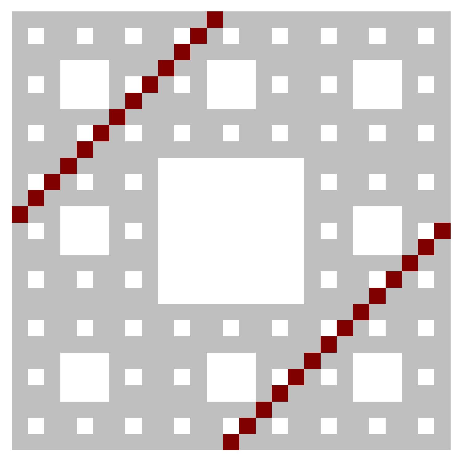
Figure 14. A discrete Sierpiński carpet $\mathcal{C}_{k,\mathcal{A}}$, with $M:=3$, $\mathcal{A}:=\{0,1,2\}^{2}\setminus\{(1,1)\}$; in the picture we have $k=3$. The dark red line is the diagonal $\{(j,j+{3^{k}-1\over 2})\mid j=0,\dots,3^{k}-1\}$ contained in $\mathcal{C}_{k,\mathcal{A}}$.

Conjecture 6.7.

The bound (6.7) holds with some $\beta>0$ (by Lemma 6.4 this is the same as saying that the left-hand side of (6.7) is $<1$ for some value of $k$) unless one of the following situations happens:

1. one of the sets $\mathcal{A},\mathcal{B}$ contains a horizontal line and the other set contains a vertical line, or

2. for each $k$, one of the sets $\mathcal{C}_{k,\mathcal{A}},\mathcal{C}_{k,\mathcal{B}}$ contains a diagonal line and the other set contains an antidiagonal line.

Here a horizontal line in $\mathbb{Z}_{M}^{2}$ is defined as a set of the form $\{(j,s)\mid j\in\mathbb{Z}_{M}\}$ for some $s\in\mathbb{Z}_{M}$; a vertical line is defined similarly, replacing $(j,s)$ with $(s,j)$. A diagonal line in $\mathbb{Z}_{N}^{2}$ is defined as a set of the form $\{(j,(j+s)\bmod N)\mid j\in\mathbb{Z}_{N}\}$ for some $s\in\mathbb{Z}_{N}$; an antidiagonal line is defined similarly, replacing $j+s$ by $s-j$. If either case (1) or case (2) above hold, then one can show that the norm in (6.7) is equal to 1. We note that the case (2) in Conjecture 6.7 can arise in a non-obvious way, see Figure 14.

We finish this section with two conditions under which (6.7) is known to hold with some $\beta>0$. The first one says that the complement of $\mathcal{A}$ contains a vertical line, while $\mathcal{B}$ contains no horizontal line:

Proposition 6.8.

Assume that (see Figure 15):

1. there exists $s\in\mathbb{Z}_{M}$ such that $(s,j)\notin\mathcal{A}$ for all $j\in\mathbb{Z}_{M}$, and

2. for each $t\in\mathbb{Z}_{M}$, the set $\{\ell\mid(\ell,t)\in\mathcal{B}\}$ is not equal to the entire $\mathbb{Z}_{M}$.

Then (6.7) holds with some $\beta>0$.

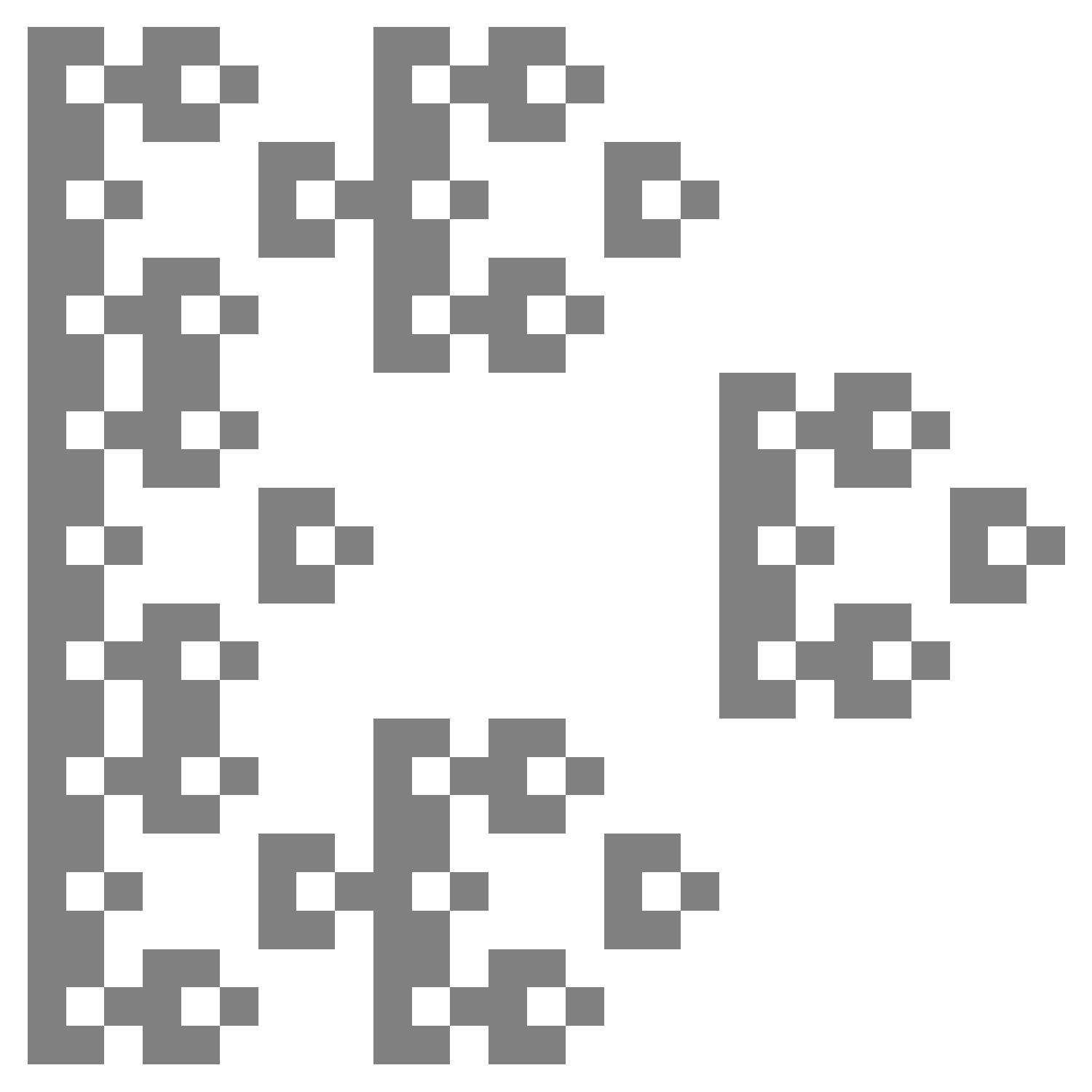
$\mathcal{C}_{k,\mathcal{A}}$     $\mathcal{C}_{k,\mathcal{B}}$

Figure 15. An example of Cantor sets with $M=3$, $k=3$ satisfying the conditions of Proposition 6.8.

Proof.

By Lemma 6.4, it suffices to show that the left-hand side of (6.7) is $<1$ for some value of $k$. We argue by contradiction, assuming that this left-hand side is equal to 1. Similarly to Lemma 4.7, there then exists nonzero $u\in\mathbb{C}^{N\times N}$ such that

$$\operatorname{supp}u\subset\mathcal{C}_{k,\mathcal{B}},\quad\operatorname{supp}(\mathcal{F}_{N\times N}u)\subset\mathcal{C}_{k,\mathcal{A}}.$$ (6.9)

For every $\ell_{2}\in\mathbb{Z}_{N}$, define $u_{\ell_{2}}\in\mathbb{C}^{N}$ by $u_{\ell_{2}}(\ell_{1})=u(\ell_{1},\ell_{2})$. Denote by $\mathcal{D}\subset\mathbb{Z}_{N}$ the set of all numbers of the form $d_{0}+d_{1}M+\dots+d_{k-1}M^{k-1}$ where $d_{0},d_{1},\dots,d_{k-1}\neq s$. Then by condition (1) the projection of $\operatorname{supp}\mathcal{F}_{N\times N}u$ onto the first coordinate lies inside $\mathcal{D}$. Writing

$$\mathcal{F}_{N}u_{\ell_{2}}(j_{1})={1\over\sqrt{N}}\sum_{j_{2}=0}^{N-1}\exp\Big{(}{2\pi ij_{2}\ell_{2}\over N}\Big{)}\mathcal{F}_{N\times N}u(j_{1},j_{2})$$

we see that

$$\operatorname{supp}(\mathcal{F}_{N}u_{\ell_{2}})\subset\mathcal{D}\quad\text{for all}\quad\ell_{2}\in\mathbb{Z}_{N}.$$

In particular, $\operatorname{supp}(\mathcal{F}_{N}u_{\ell_{2}})$ does not intersect some interval of length $M^{k-1}$. Arguing as in the proof of Lemma 4.7 we see that

$$\text{for each }\ell_{2}\in\mathbb{Z}_{N},\quad\text{either }\operatorname{supp}u_{\ell_{2}}=\emptyset\quad\text{or }\#(\operatorname{supp}u_{\ell_{2}})>M^{k-1}.$$ (6.10)

On the other hand, by condition (2) the support of each $u_{\ell_{2}}$ has at most $(M-1)^{k}$ elements. Choosing $k$ large enough so that $(M-1)^{k}\leq M^{k-1}$ we get that $u\equiv 0$, giving a contradiction. ∎

The second condition can be viewed as a special case of the work of Han–Schlag [HS18] presented in §6.1, letting $\mathcal{B}$ be any alphabet not equal to the entire $\mathbb{Z}_{M}^{2}$ and requiring that the complement of $\mathcal{A}$ contain both a horizontal and a vertical line:

Proposition 6.9.

Assume that (see Figure 16):

1. there exist $s,t\in\mathbb{Z}_{M}$ such that $(s,j)\notin\mathcal{A}$ and $(j,t)\notin\mathcal{A}$ for all $j$, and

2. $\mathcal{B}$ is not equal to the entire $\mathbb{Z}_{M}^{2}$.

Then (6.7) holds with some $\beta>0$.

$\mathcal{C}_{k,\mathcal{A}}$     $\mathcal{C}_{k,\mathcal{B}}$

Figure 16. An example of Cantor sets with $M=3$, $k=3$ satisfying the conditions of Proposition 6.9.

Proof.

We argue similarly to the proof of Proposition 6.8, assuming the existence of nonzero $u$ satisfying (6.9). By the first part of condition (1) we see that $\operatorname{supp}u$ satisfies (6.10); that is, the intersection of $\operatorname{supp}u$ with each horizontal line is either empty or contains $>M^{k-1}$ points. We fix $k_{0}\geq 0$ such that

$$\Big{(}1-{1\over M}\Big{)}^{k_{0}}\leq{1\over M}$$ (6.11)

and take $k\geq k_{0}$. By condition (2) there exists $(s^{\prime},t^{\prime})\in\mathbb{Z}_{M}^{2}\setminus\mathcal{B}$. For $b=b_{0}+b_{1}M+\dots+b_{k-1}M^{k-1}$, where $b_{0},\dots,b_{k-1}\in\mathbb{Z}_{M}$, we say that $b$ is thin if at most $k_{0}$ digits $b_{0},\dots,b_{k-1}$ are equal to $t^{\prime}$, and thick otherwise.

If $b$ is thick, then the set $\{a\in\mathbb{Z}_{N}\mid(a,b)\in\operatorname{supp}u\}$ contains at most $(M-1)^{k_{0}}M^{k-k_{0}}$ points. Indeed, writing $b$ as above and $a=a_{0}+a_{1}M+\dots+a_{k-1}M^{k-1}$, if $(a,b)\in\operatorname{supp}u\subset\mathcal{C}_{k,\mathcal{B}}$, then for each $r=0,\dots,k-1$ we have $(a_{r},b_{r})\neq(s^{\prime},t^{\prime})$. Since $b$ is thick, there exist $r_{1}<r_{2}<\dots<r_{k_{0}}$ such that $b_{r_{1}}=\dots=b_{r_{k_{0}}}=t^{\prime}$. Then $a$ has to satisfy the conditions $a_{r_{1}},\dots,a_{r_{k_{0}}}\neq s^{\prime}$, and the number of such points $a$ is equal to $(M-1)^{k_{0}}M^{k-k_{0}}$.

By (6.11) we have $(M-1)^{k_{0}}M^{k-k_{0}}\leq M^{k-1}$. Then by (6.10) we see that for each thick $b$, the intersection of $\operatorname{supp}u$ with the horizontal line $\{(a,b)\mid a\in\mathbb{Z}_{N}\}$ is empty. Thus the projection $\pi_{2}(\operatorname{supp}u)$ of $\operatorname{supp}u$ onto the second coordinate is contained inside the set of all thin elements of $\mathbb{Z}_{N}$, giving

$$\#(\pi_{2}(\operatorname{supp}u))\leq\binom{k}{k_{0}}M^{k_{0}}(M-1)^{k-k_{0}}.$$ (6.12)

On the other hand, using the second part of condition (1) similarly to (6.10) we see that the intersection of $\operatorname{supp}u$ with each vertical line is either empty or contains $>M^{k-1}$ points. Choose $k$ large enough (depending on $k_{0}$) so that the left-hand side of (6.12) is $\leq M^{k-1}$. Then we see that $u\equiv 0$, giving a contradiction. ∎

Acknowledgements. The author was supported by the NSF CAREER grant DMS-1749858 and a Sloan Research Fellowship. Part of this article originated as lecture notes for the minicourse on fractal uncertainty principle at the Third Symposium on Scattering and Spectral Theory in Florianopolis, Brazil, July 2017, and another part as lecture notes for the Emerging Topics Workshop on quantum chaos and fractal uncertainty principle at the Institute for Advanced Study, Princeton, October 2017. The numerics used to plot Figures 2, 5, and 13 were originally developed for an undergraduate project at MIT joint with Arjun Khandelwal during the 2015–2016 academic year. The author thanks the anonymous referee for a careful reading of the manuscript and many suggestions to improve the presentation.

References

- [An08] Nalini Anantharaman, Entropy and the localization of eigenfunctions, Ann. of Math. 168(2008), 435–475.
- [AN07] Nalini Anantharaman and Stéphane Nonnenmacher, Half-delocalization of eigenfunctions of the Laplacian on an Anosov manifold, Ann. Inst. Fourier 57(2007), 2465–2523.
- [B∗13] Sonja Barkhofen, Tobias Weich, Alexander Potzuweit, Hans-Jürgen Stöckmann, Ulrich Kuhl, and Maciej Zworski, Experimental observation of the spectral gap in microwave -disk systems, Phys. Rev. Lett. 110(2013), 164102.
- [BM62] Arne Beurling and Paul Malliavin, On Fourier transforms of measures with compact support, Acta Math. 107(1962), 291–309.
- [Bo14] David Borthwick, Distribution of resonances for hyperbolic surfaces, Experimental Math. 23(2014), 25–45.
- [Bo16] David Borthwick, Spectral theory of infinite-area hyperbolic surfaces, second edition, Birkhäuser, 2016.
- [BW16] David Borthwick and Tobias Weich, Symmetry reduction of holomorphic iterated function schemes and factorization of Selberg zeta functions, J. Spectr. Th. 6(2016), 267–329.
- [BD17] Jean Bourgain and Semyon Dyatlov, Fourier dimension and spectral gaps for hyperbolic surfaces, Geom. Funct. Anal. 27(2017), 744–771.
- [BD18] Jean Bourgain and Semyon Dyatlov, Spectral gaps without the pressure condition, Ann. Math. (2) 187(2018), 825–867.
- [BGS11] Jean Bourgain, Alex Gamburd, and Peter Sarnak, Generalization of Selberg’s 3/16 theorem and affine sieve, Acta Math. 207(2011), 255–290.
- [BGH10] Nicolas Burq, Colin Guillarmou, and Andrew Hassell, Strichartz estimates without loss on manifolds with hyperbolic trapped geodesics, Geom. Funct. Anal. 20(2010), 627–656.
- [CdV85] Yves Colin de Verdière, Ergodicité et fonctions propres du Laplacien, Comm. Math. Phys. 102(1985), 497–502.
- [Do98] Dmitry Dolgopyat, On decay of correlations in Anosov flows, Ann. Math. (2) 147(1998), 357–390.
- [Dy17] Semyon Dyatlov, Control of eigenfunctions on hyperbolic surfaces: an application of fractal uncertainty principle, Journées équations aux dérivées partielles (2017), Exp. No. 4.
- [Dy18] Semyon Dyatlov, Notes on hyperbolic dynamics, preprint, arXiv:1805.11660.
- [DJ17] Semyon Dyatlov and Long Jin, Resonances for open quantum maps and a fractal uncertainty principle, Comm. Math. Phys. 354(2017), 269–316.
- [DJ18a] Semyon Dyatlov and Long Jin, Dolgopyat’s method and the fractal uncertainty principle, Analysis&PDE 11(2018), 1457–1485.
- [DJ18b] Semyon Dyatlov and Long Jin, Semiclassical measures on hyperbolic surfaces have full support, Acta Math. 220(2018), 297–339.
- [DJN19] Semyon Dyatlov, Long Jin, and Stéphane Nonnenmacher, Control of eigenfunctions on surfaces of variable curvature, preprint, arXiv:1906.08923.
- [DZ16] Semyon Dyatlov and Joshua Zahl, Spectral gaps, additive energy, and a fractal uncertainty principle, Geom. Funct. Anal. 26(2016), 1011–1094.
- [DZ17] Semyon Dyatlov and Maciej Zworski, Fractal uncertainty for transfer operators, Int. Math. Res. Not., published online.
- [DZ19] Semyon Dyatlov and Maciej Zworski, Mathematical theory of scattering resonances, Graduate Studies in Mathematics 200, AMS, 2019.
- [GR89] Pierre Gaspard and Stuart Rice, Scattering from a classically chaotic repeller, J. Chem. Phys. 90(1989), 2225–2241.
- [HS18] Rui Han and Wilhelm Schlag, A higher dimensional Bourgain-Dyatlov fractal uncertainty principle, to appear in Analysis&PDE, arXiv:1805.04994.
- [Ha89] Alain Haraux, Séries lacunaires et contrôle semi-interne des vibrations d’une plaque rectangulaire, J. Math. Pures Appl. 68(1989), 457–465.
- [HV18] Peter Hintz and András Vasy, The global non-linear stability of the Kerr–de Sitter family of black holes, Acta Math. 220(2018), 1–206.
- [Ik88] Mitsuru Ikawa, Decay of solutions of the wave equation in the exterior of several convex bodies, Ann. Inst. Fourier 38(1988), 113–146.
- [Ja90] Stéphane Jaffard, Contrôle interne exact des vibrations d’une plaque rectangulaire, Portugal. Math. 47(1990), 423–429.
- [Ja97] Dmitry Jakobson, Quantum limits on flat tori, Ann. of Math. 145(1997), 235–266.
- [JN10] Dmitry Jakobson and Frédéric Naud, Lower bounds for resonances of infinite-area Riemann surfaces, Anal. PDE 3(2010), 207–225.
- [Ji17] Long Jin, Damped wave equations on compact hyperbolic surfaces, preprint, arXiv:1712.02692.
- [Ji18] Long Jin, Control for Schrödinger equation on hyperbolic surfaces, Math. Res. Lett. 25(2018), 1865–1877.
- [JZ17] Long Jin and Ruixiang Zhang, Fractal uncertainty principle with explicit exponent, preprint, arXiv:1710.00250.
- [JS16] Thomas Jordan and Tuomas Sahlsten, Fourier transforms of Gibbs measures for the Gauss map, Math. Ann., 364(2016), 983–1023.
- [Li18] Jialun Li, Fourier decay, renewal theorem and spectral gaps for random walks on split semisimple Lie groups, preprint, arXiv:1811.06484.
- [LNP19] Jialun Li, Frédéric Naud, and Wenyu Pan, Kleinian Schottky groups, Patterson-Sullivan measures and Fourier decay, preprint, arXiv:1902.01103.
- [Li06] Elon Lindenstrauss, Invariant measures and arithmetic quantum unique ergodicity, Ann. of Math. 163(2006), 165–219.
- [Li88] Jacques-Louis Lions, Contrôlabilité exacte, perturbation et stabilisation des systèmes distribués, R.M.A. Masson 23(1988).
- [MOW16] Michael Magee, Hee Oh, and Dale Winter, Uniform congruence counting for Schottky semigroups in , with an appendix by Jean Bourgain, Alex Kontorovich, and Michael Magee, J. für die reine und angewandte Mathematik, published online.
- [Ma06] Jens Marklof, Arithmetic quantum chaos, Encyclopedia of Mathematical Physics, Oxford: Elsevier 1(2006), 212–220.
- [Na05] Frédéric Naud, Expanding maps on Cantor sets and analytic continuation of zeta functions, Ann. de l’ENS (4) 38(2005), 116–153.
- [No11] Stéphane Nonnenmacher, Spectral problems in open quantum chaos, Nonlinearity 24(2011), R123.
- [NZ09] Stéphane Nonnenmacher and Maciej Zworski, Quantum decay rates in chaotic scattering, Acta Math. 203(2009), 149–233.
- [Pa76] Samuel James Patterson, The limit set of a Fuchsian group, Acta Math. 136(1976), 241–273.
- [PS10] Vesselin Petkov and Luchezar Stoyanov, Analytic continuation of the resolvent of the Laplacian and the dynamical zeta function, Anal. PDE 3(2010), 427–489.
- [RS94] Zeév Rudnick and Peter Sarnak, The behaviour of eigenstates of arithmetic hyperbolic manifolds, Comm. Math. Phys. 161(1994), 195–213.
- [SS18] Tuomas Sahlsten and Connor Stevens, Fourier decay in nonlinear dynamics, preprint, arXiv:1810.01378.
- [Sa11] Peter Sarnak, Recent progress on the quantum unique ergodicity conjecture, Bull. Amer. Math. Soc. 48(2011), 211–228.
- [Sa13] Peter Sarnak, Notes on thin matrix groups, MSRI Publications 61(2013).
- [Sh74a] Alexander Shnirelman, Ergodic properties of eigenfunctions, Usp. Mat. Nauk. 29(1974), 181–182.
- [Sh74b] Alexander Shnirelman, Statistical properties of eigenfunctions, Proceedings of the All-USSR School on differential equations with infinitely many independent variables and dynamical systems with infinitely many degrees of freedom, Dilijan, Armenia, May 21–June 3, 1973; Armenian Academy of Sciences, Erevan, 1974.
- [St11] Luchezar Stoyanov, Spectra of Ruelle transfer operators for axiom A flows, Nonlinearity 24(2011), 1089–1120.
- [St12] Luchezar Stoyanov, Non-integrability of open billiard flows and Dolgopyat-type estimates, Erg. Theory Dyn. Syst. 32(2012), 295–313.
- [SU13] Alexander Strohmaier and Ville Uski, An algorithm for the computation of eigenvalues, spectral zeta functions and zeta-determinants on hyperbolic surfaces, Comm. Math. Phys. 317(2013), 827–869.
- [Su79] Dennis Sullivan, The density at infinity of a discrete group of hyperbolic motions, Publ. Math. de l’IHES 50(1979), 171–202.
- [Va13a] András Vasy, Microlocal analysis of asymptotically hyperbolic and Kerr–de Sitter spaces, with an appendix by Semyon Dyatlov, Invent. Math. 194(2013), 381–513.
- [Va13b] András Vasy, Microlocal analysis of asymptotically hyperbolic spaces and high energy resolvent estimates, Inverse Problems and Applications. Inside Out II, Gunther Uhlmann (ed.), MSRI publications 60, Cambridge Univ. Press, 2013.
- [Wa17] Jian Wang, Strichartz estimates for convex co-compact hyperbolic surfaces, Proc. Amer. Math. Soc. 147(2019), 873–883.
- [Ze87] Steve Zelditch, Uniform distribution of eigenfunctions on compact hyperbolic surfaces, Duke Math. J. 55(1987), 919–941.
- [Ze09] Steve Zelditch, Recent developments in mathematical quantum chaos, Curr. Dev. Math. 2009, 115–204.
- [Zw12] Maciej Zworski, Semiclassical analysis, Graduate Studies in Mathematics 138, AMS, 2012.
- [Zw17] Maciej Zworski, Mathematical study of scattering resonances, Bull. Math. Sci. (2017) 7:1–85.