Dynamic NE Seeking for Multi-Integrator Networked Agents with Disturbance Rejection

Andrew R. Romano and Lacra Pavel This work was supported by NSERC Grant (261764). A.R. Romano and L. Pavel are with Department of Electrical and Computer Engineering, University of Toronto, Canada. andrew.romano@mail.utoronto.ca, pavel@ece.utoronto.ca
Abstract

In this paper, we consider game problems played by (multi)-integrator agents, subject to external disturbances. We propose Nash equilibrium seeking dynamics based on gradient-play, augmented with a dynamic internal-model based component, which is a reduced-order observer of the disturbance. We consider single-, double- and extensions to multi-integrator agents, in a partial-information setting, where agents have only partial knowledge on the others’ decisions over a network. The lack of global information is offset by each agent maintaining an estimate of the others’ states, based on local communication with its neighbours. Each agent has an additional dynamic component that drives its estimates to the consensus subspace. In all cases, we show convergence to the Nash equilibrium irrespective of disturbances. Our proofs leverage input-to-state stability under strong monotonicity of the pseudo-gradient and Lipschitz continuity of the extended pseudo-gradient.

I Introduction

Game theory has found many applications in multi-agent engineering problems, wherein each agent can be modelled as an independent, selfish decision maker that tries to optimize its individual, but coupled, cost function. These include wireless communication networks [1], [2], [3], optical networks [4], [5], smart-grid and PEV charging [6], [7], [8] noncooperative flow control [9], [10] and multi-agent formation problems[11]. The relevant equilibrium sought is the Nash equilibrium (NE), whereby no agent has incentive to unilaterally change its action. The objective is to design either continuous-time or discrete-time, distributed learning schemes that converge to the NE under reasonable assumptions on the game properties and agent knowledge. Most works focus on algorithms for agents that either do not have dynamics, or have single integrator dynamics, and disturbances are not explicitly considered, [12].

There are many scenarios when the game or the agents are subject to disturbances, noise or uncertainties. Examples are demand-side management in smart-grids, with changes in the energy consumption demand, [6], feedback control for PEV charging load allocation, [8], or power control for optical-signal-to-noise ratio (OSNR) in the presence of pilot tones, [13]. Yet there have been relatively few works on Nash equilibrium seeking in such settings. In [8], a time-varying pricing function that affects the cost functions of each agent is considered. Only robustness to the time-varying component is investigated. Another good motivating example is the case of a group of mobile robots in a sensor network, similar to the examples in [14]. Each agent in the network has a goal related to its global position. However, it must also consider its position relative to the other agents in the network in order to make sure that it maintains communication with its neighbours. This can easily be formulated as a game played by the robots, which can be modelled as higher-order agents. In addition, each robot may be subject to a disturbance, e.g., wind or a slope in the terrain. It is important that these robots be able to reject this deterministic disturbance and still converge to the NE. A similar problem without disturbances was presented in [15], however the state space is discretized and the game is treated as a finite action game. This formulation ignores the dynamics of the individual agents.

Motivated by the above, in this paper our focus is to extend these results to games wherein the agents are modelled as (multi)-integrator systems subject to external deterministic disturbances. This is related to NE seeking with noisy feedback, on which there has been recent work. A dual-averaging algorithm with noisy gradients is considered in [16]. A discrete-time extremum seeking algorithm with noisy cost measurements for agents modelled as single and double integrators and kinematic unicycles is investigated in [14]. In both of these papers, the noise involved is stochastic in nature instead of a deterministic disturbance, as we consider here. Separately, NE seeking in the special class of aggregative games for Euler-Lagrange systems has been recently investigated in [17], which is similar to our work due to the dynamic nature of the agents involved, but without disturbances being considered.

Our work is related to the literature on disturbance rejection and tracking in multi-agent systems, [18], [19], [20], [21], [22]. Most output regulation problems in multi-agent systems can be viewed as specific cases of game theoretical problems. The synchronization problem, for example, can be regarded as a special game where each agent’s cost function is quadratic and corresponds to the sum of the squared distances to all of its neighbours.

Our work is also related to distributed optimization, where a group of agents cooperatively minimize a global cost function, the sum of the agents’ individual cost functions. Optimization schemes that reject disturbances have been discussed for single integrator systems [23], systems with unit relative degree [24] and systems with double integrator dynamics [25]. In [26] the robustness of a continuous-time distributed optimization algorithm is analyzed in the presence of additively persistent noise on agents’ communication and computation, in a directed communication graph. Key differences from a game setup are the cooperative nature of the problem and the fact that usually each agent’s cost is decoupled of the others’ variables. Exploiting summability, leads to a set of parallel decoupled optimization problems, one for each agent and its own cost function. Even when the overall cost is not separable, due to its summable structure, one can extend the problem to an augmented space of estimates, where it becomes separable and convex. In a game context, an agent’s cost is inherently coupled to the others’ decisions, on which it does not have control and convexity is only partial.

Contributions. Motivated by the above, in this paper we consider how to design Nash equilibrium seeking dynamics that simultaneously reject exogenous disturbances. We consider single and double-integrator agents, i.e., agents that behave as continuous-time dynamical systems that integrate their respective inputs, in a partial-information setting, i.e., networked regimes where agents may only access the states of their neighbours. We also discuss extensions to multi-integrator agents. Unlike multi-agent set stabilization problems with disturbance rejection, herein the stabilization goal is the a priori unknown Nash equilibrium of the game, which has to be reached irrespective of disturbances. In all cases, we make standard assumptions that provide existence and uniqueness of the NE of the game.

Due to the partial-information setting, we inspire from the disturbance-free results in [27]. Each player keeps track of an estimate of the others’ decisions as in [27], and the problem can be seen as one of multi-agent agreement with disturbance rejection. The agreement subspace is the estimate-consensus subspace at the Nash equilibrium, irrespective of the disturbance. The proposed agent learning dynamics has two components: a gradient-play with estimate consensus component (that drives each player’s dynamics towards minimizing its own cost function) and a dynamic internal-model component, which effectively implements a reduced-order observer of the disturbance. Unlike typical multi-agent agreement, [18], [19], [21], we cannot use individual passivity of each agent. Rather, our proofs rely on combining input-to-state stability with design of a reduced-observer for disturbance, under strong monotonicity of the pseudo-gradient and Lipschitz continuity of the extended pseudo-gradient. The resulting agent dynamics are locally distributed, with coupling introduced only through the communication graph.

The paper is organized as follows. In Section II, we give the necessary background on nonlinear systems, graph theory and noncooperative game theory. In Section III, we formulate the NE seeking problem for dynamic agents with disturbance rejection. In Section IV, we give our results for NE seeking dynamics with disturbance rejection for single-integrator agents. In Section V, we formulate a NE seeking algorithm for double-integrator agents and discuss extensions to multi-integrator agents. In Section VI, we compare by simulation their performance with those of a standard gradient-play dynamics and an augmented gradient-play dynamics with estimate consensus (partial information setting), and give conclusions in Section VII. A short version of this work appeared in [28], where only single-integrators are treated.

Notations. Let \mathbb{R}, 0subscriptabsent0\mathbb{R}_{\geq 0} denote the set of real and non-negative real numbers, \mathbb{C} and superscript\mathbb{C}^{-} the set of complex numbers and complex numbers with negative real part. Given x,yn𝑥𝑦superscript𝑛x,y\!\in\!\mathbb{R}^{n}, xTysuperscript𝑥𝑇𝑦x^{T}y denotes the inner product of x𝑥x and y𝑦y. Let :n0\|\cdot\|\!:\!\mathbb{R}^{n}\!\rightarrow\!\mathbb{R}_{\geq 0} denote the Euclidean norm and :m×n0\|\cdot\|\!:\!\mathbb{R}^{m\times n}\!\rightarrow\!\mathbb{R}_{\geq 0} denote the induced matrix norm. col(x1,,xN)colsubscript𝑥1subscript𝑥𝑁\operatorname{col}(x_{1},\dots,x_{N}) denotes [x1T,,xNT]Tsuperscriptsuperscriptsubscript𝑥1𝑇superscriptsubscript𝑥𝑁𝑇𝑇[x_{1}^{T},\dots,x_{N}^{T}]^{T}. Given matrices A1,,ANsubscript𝐴1subscript𝐴𝑁A_{1},\dots,A_{N}, blkdiag(A1,,AN)blkdiagsubscript𝐴1subscript𝐴𝑁\operatorname{blkdiag}(A_{1},\dots,A_{N}) denotes the block diagonal matrix with Aisubscript𝐴𝑖A_{i} on the diagonal. Insubscript𝐼𝑛I_{n} denotes the n×n𝑛𝑛n\!\times\!n identity matrix. 𝟏nsubscript1𝑛\boldsymbol{1}_{n} denotes the n×1𝑛1n\!\times\!1 all ones vector. ABtensor-product𝐴𝐵A\otimes B denotes the Kronecker product of matrices A𝐴A and B𝐵B.

II Background

II-A Input to State Stability

In this work, we model the dynamics of each agent as a continuous time dynamical system. We first introduce some background from [29]. Consider a nonlinear system,

x˙=f(x,u)˙𝑥𝑓𝑥𝑢\displaystyle\dot{x}=f(x,u) (1)

where x˙:=dx(t)dtassign˙𝑥𝑑𝑥𝑡𝑑𝑡\dot{x}:=\frac{dx(t)}{dt}, f:n×mn:𝑓superscript𝑛superscript𝑚superscript𝑛f\!:\!\mathbb{R}^{n}\!\times\!\mathbb{R}^{m}\!\rightarrow\!\mathbb{R}^{n} is locally Lipschitz in x𝑥x and u𝑢u and the input u(t)𝑢𝑡u(t) is a piecewise continuous, bounded function.

Definition 1

System (1) is input-to-state stable (ISS) if there exist β𝒦𝛽𝒦\beta\in\mathcal{KL} and γ𝒦𝛾𝒦\gamma\in\mathcal{K} such that for any initial state x(t0)𝑥subscript𝑡0x(t_{0}) and any bounded input u(t)𝑢𝑡u(t), the solution x(t)𝑥𝑡x(t) satisfies

x(t)β(x(t0),tt0)+γ(suptoτtu(τ)),tt0formulae-sequencenorm𝑥𝑡𝛽norm𝑥subscript𝑡0𝑡subscript𝑡0𝛾subscriptsupremumsubscript𝑡𝑜𝜏𝑡norm𝑢𝜏for-all𝑡subscript𝑡0\displaystyle\|x(t)\|\leq\beta(\|x(t_{0})\|,t-t_{0})+\gamma\Big{(}\sup_{t_{o}\leq\tau\leq t}\|u(\tau)\|\Big{)},\,\,\forall t\geq t_{0}
Theorem 1

(Theorem 4.19, [29]) Let V(x)𝑉𝑥V(x) be a continuously differentiable function such that

α1(x)subscript𝛼1norm𝑥\displaystyle\alpha_{1}(\|x\|) V(x)α2(x)absent𝑉𝑥subscript𝛼2norm𝑥\displaystyle\leq V(x)\leq\alpha_{2}(\|x\|)
Vxf(x,u)𝑉𝑥𝑓𝑥𝑢\displaystyle\frac{\partial V}{\partial x}f(x,u) W(x),xρ(u)>0formulae-sequenceabsent𝑊𝑥for-allnorm𝑥𝜌norm𝑢0\displaystyle\leq-W(x),\ \forall\|x\|\geq\rho(\|u\|)>0

xn,umformulae-sequencefor-all𝑥superscript𝑛𝑢superscript𝑚\forall x\!\in\!\mathbb{R}^{n},\ u\!\in\!\mathbb{R}^{m}, where α1,α2𝒦,ρ𝒦formulae-sequencesubscript𝛼1subscript𝛼2subscript𝒦𝜌𝒦\alpha_{1},\alpha_{2}\!\in\!\mathcal{K}_{\infty},\!\rho\!\in\!\mathcal{K}, and W(x)𝑊𝑥W(x) is positive definite. Then system (1) is ISS with γ=α11α2ρ𝛾superscriptsubscript𝛼11subscript𝛼2𝜌\gamma\!=\!\alpha_{1}^{-1}\!\circ\!\alpha_{2}\!\circ\!\rho.

Consider now the cascade of two systems

x˙1subscript˙𝑥1\displaystyle\dot{x}_{1} =f1(x1,x2)absentsubscript𝑓1subscript𝑥1subscript𝑥2\displaystyle=f_{1}(x_{1},x_{2}) (2)
x˙2subscript˙𝑥2\displaystyle\dot{x}_{2} =f2(x2)absentsubscript𝑓2subscript𝑥2\displaystyle=f_{2}(x_{2}) (3)

with f1:n1×n2n1:subscript𝑓1superscriptsubscript𝑛1superscriptsubscript𝑛2superscriptsubscript𝑛1f_{1}\!:\!\mathbb{R}^{n_{1}}\!\times\!\mathbb{R}^{n_{2}}\!\rightarrow\!\mathbb{R}^{n_{1}}, f2:n2n2:subscript𝑓2superscriptsubscript𝑛2superscriptsubscript𝑛2f_{2}\!:\!\mathbb{R}^{n_{2}}\!\rightarrow\!\mathbb{R}^{n_{2}} locally Lipschitz.

Lemma 1

(Lemma 4.7, [29]) If the system (2) with x2subscript𝑥2x_{2} as an input is ISS and the origin of (3) is globally uniformly asymptotically stable, then the origin of the cascade system (2) and (3) is globally uniformly asymptotically stable.

II-B Graph Theory

In this paper, we consider NE seeking for dynamic agents with communication over networks with fixed (static) topology. The communication protocol relies on graph theory. The following is from [30]. An undirected graph, G𝐺G is a pair G=(,E)𝐺𝐸G=(\mathcal{I},E) where ={1,,N}1𝑁\mathcal{I}=\{1,\dots,N\} is the vertex set and E×𝐸E\subset\mathcal{I}\times\mathcal{I} is the edge set. Since G𝐺G is an undirected graph, for all i,j𝑖𝑗i,j\in\mathcal{I}, if (i,j)E𝑖𝑗𝐸(i,j)\in E then (j,i)E𝑗𝑖𝐸(j,i)\in E. Let 𝒩isubscript𝒩𝑖\mathcal{N}_{i}\subset\mathcal{I} denote the set of neighbours of player i𝑖i. The adjacency matrix A=[aij]N×NAdelimited-[]subscript𝑎𝑖𝑗superscript𝑁𝑁\textbf{A}=[a_{ij}]\in\mathbb{R}^{N\times N} of the graph G𝐺G is defined such that aij=1subscript𝑎𝑖𝑗1a_{ij}=1 if (j,i)E𝑗𝑖𝐸(j,i)\in E and aij=0subscript𝑎𝑖𝑗0a_{ij}=0 otherwise. For an an undirected graph, aij=ajisubscript𝑎𝑖𝑗subscript𝑎𝑗𝑖a_{ij}=a_{ji}. G𝐺G is connected if any two agents are connected by a path. The Laplacian matrix L=[lij]N×N𝐿delimited-[]subscript𝑙𝑖𝑗superscript𝑁𝑁L=[l_{ij}]\in\mathbb{R}^{N\times N} of the graph G𝐺G is defined as lii=jiaij=|𝒩i|subscript𝑙𝑖𝑖subscript𝑗𝑖subscript𝑎𝑖𝑗subscript𝒩𝑖l_{ii}=\sum_{j\neq i}a_{ij}=|\mathcal{N}_{i}| and lij=aijsubscript𝑙𝑖𝑗subscript𝑎𝑖𝑗l_{ij}=-a_{ij}, for ij𝑖𝑗i\neq j. For an undirected and connected graph, L𝐿L is symmetric positive definite and has a simple zero eigenvalue such that 0<λ2(L)λN(L)0subscript𝜆2𝐿subscript𝜆𝑁𝐿0<\lambda_{2}(L)\leq\ldots\leq\lambda_{N}(L) and L1N=0𝐿subscript1𝑁0L\textbf{1}_{N}=0. Furthermore, for any vector yN𝑦superscript𝑁y\in\mathbb{R}^{N} satisfying 1NTy=0superscriptsubscript1𝑁𝑇𝑦0\textbf{1}_{N}^{T}y=0, λ2(L)y2yTLyλN(L)y2subscript𝜆2𝐿superscriptnorm𝑦2superscript𝑦𝑇𝐿𝑦subscript𝜆𝑁𝐿superscriptnorm𝑦2\lambda_{2}(L)\|y\|^{2}\leq y^{T}Ly\leq\lambda_{N}(L)\|y\|^{2}.

II-C Game Theory

Consider a set of players, ={1,,N}1𝑁\mathcal{I}=\{1,\dots,N\}. Each player i𝑖i\in\mathcal{I} controls its own action xiΩinisubscript𝑥𝑖subscriptΩ𝑖superscriptsubscript𝑛𝑖x_{i}\in\Omega_{i}\subset\mathbb{R}^{n_{i}}. The overall action set of the players is Ω=Ω1××ΩNnΩsubscriptΩ1subscriptΩ𝑁superscript𝑛\Omega=\Omega_{1}\times\dots\times\Omega_{N}\subset\mathbb{R}^{n}, where n=ini𝑛subscript𝑖subscript𝑛𝑖n=\sum_{i\in\mathcal{I}}n_{i}. Let x=(xi,xi)Ω𝑥subscript𝑥𝑖subscript𝑥𝑖Ωx=(x_{i},x_{-i})\in\Omega denote the overall action profile of all players, where xiΩi=Ω1××Ωi1×Ωi+1××ΩNnisubscript𝑥𝑖subscriptΩ𝑖subscriptΩ1subscriptΩ𝑖1subscriptΩ𝑖1subscriptΩ𝑁superscriptsubscript𝑛𝑖{\color[rgb]{0,0,1}\definecolor[named]{pgfstrokecolor}{rgb}{0,0,1}x_{-i}}\in\Omega_{-i}=\Omega_{1}\times\dots\times\Omega_{i-1}\times\Omega_{i+1}\times\dots\times\Omega_{N}\subset\mathbb{R}^{n_{-i}} is the action set of all players except for player i𝑖i. Let Ji:Ω:subscript𝐽𝑖ΩJ_{i}:\Omega\rightarrow\mathbb{R} be the cost function of player i𝑖i. Each player tries to minimize its own cost function over its action. Denote the game 𝒢(,Ji,Ωi)𝒢subscript𝐽𝑖subscriptΩ𝑖\mathcal{G}(\mathcal{I},J_{i},\Omega_{i}).

Definition 2

Given a game 𝒢(,Ji,Ωi)𝒢subscript𝐽𝑖subscriptΩ𝑖\mathcal{G}(\mathcal{I},J_{i},\Omega_{i}), an action profile x=(xi,xi)Ωsuperscript𝑥superscriptsubscript𝑥𝑖superscriptsubscript𝑥𝑖Ωx^{*}=(x_{i}^{*},x_{-i}^{*})\in\Omega is a Nash Equilibrium (NE) of 𝒢𝒢\mathcal{G} if

Ji(xi,xi)Ji(xi,xi)i,xiΩiformulae-sequencesubscript𝐽𝑖superscriptsubscript𝑥𝑖superscriptsubscript𝑥𝑖subscript𝐽𝑖subscript𝑥𝑖superscriptsubscript𝑥𝑖formulae-sequencefor-all𝑖for-allsubscript𝑥𝑖subscriptΩ𝑖\displaystyle J_{i}(x_{i}^{*},x_{-i}^{*})\leq J_{i}(x_{i},x_{-i}^{*})\quad\forall i\in\mathcal{I},\ \forall x_{i}\in\Omega_{i}

At a Nash Equilibrium no player can unilaterally decrease its cost, and thus has no incentive to switch strategies (actions) on its own.

Assumption 1

For each i𝑖i\in\mathcal{I}, let Ωi=nisubscriptΩ𝑖superscriptsubscript𝑛𝑖\Omega_{i}=\mathbb{R}^{n_{i}}, the cost function Ji:Ω:subscript𝐽𝑖ΩJ_{i}:\Omega\rightarrow\mathbb{R} be 𝒞1superscript𝒞1\mathcal{C}^{1} in its arguments and convex in xisubscript𝑥𝑖x_{i}.

Under Assumption 1, any NE satisfies

iJi(xi,xi)=0,iformulae-sequencesubscript𝑖subscript𝐽𝑖subscriptsuperscript𝑥𝑖subscriptsuperscript𝑥𝑖0for-all𝑖\displaystyle\nabla_{i}J_{i}(x^{*}_{i},x^{*}_{-i})=0,\quad\forall i\in\mathcal{I} (4)

where iJi(xi,xi)=xiJi(xi,xi)nisubscript𝑖subscript𝐽𝑖subscript𝑥𝑖subscript𝑥𝑖subscript𝑥𝑖subscript𝐽𝑖subscript𝑥𝑖subscript𝑥𝑖superscriptsubscript𝑛𝑖\nabla_{i}J_{i}(x_{i},x_{-i})=\frac{\partial}{\partial x_{i}}J_{i}(x_{i},x_{-i})\in\mathbb{R}^{n_{i}} is the partial gradient of player i𝑖i’s cost function, with respect to its own action. We denote the set of all NE in the game by

ΓNE={xn|iJi(xi,xi)=0,i\displaystyle\Gamma_{NE}=\big{\{}x\in\mathbb{R}^{n}|\nabla_{i}J_{i}(x_{i},x_{-i})=0,\,\forall i\in\mathcal{I} }}\displaystyle\big{\}} (5)

Let F(x)=col(1J1(x),,NJN(x))𝐹𝑥colsubscript1subscript𝐽1𝑥subscript𝑁subscript𝐽𝑁𝑥\!F(x)\!\!=\!\!\operatorname{col}(\!\nabla_{1}J_{1}(x),\dots,\!\nabla_{N}J_{N}(x)) denote the pseudo-gradient- the stacked vector of all partial gradients, so (4) is

F(x)=0𝐹superscript𝑥0\displaystyle F(x^{*})=0
Assumption 2

The pseudo-gradient F:Ωn:𝐹Ωsuperscript𝑛F:\Omega\rightarrow\mathbb{R}^{n} is strongly monotone, (xx)T(F(x)F(x))>μxx2superscript𝑥superscript𝑥𝑇𝐹𝑥𝐹superscript𝑥𝜇superscriptnorm𝑥superscript𝑥2(x-x^{\prime})^{T}(F(x)-F(x^{\prime}))>\mu||x-x^{\prime}||^{2}, x,xnfor-all𝑥superscript𝑥superscript𝑛\forall x,x^{\prime}\in\mathbb{R}^{n} for μ>0𝜇0\mu>0 and Lipschitz continuous, F(x)F(x)θxxnorm𝐹𝑥𝐹superscript𝑥𝜃norm𝑥superscript𝑥||F(x)-F(x^{\prime})||\leq\theta||x-x^{\prime}||, θ>0𝜃0\theta>0.

Under Assumptions 1 and 2, by Theorem 3 in [31], the game has a unique NE.

II-D Full-Information Gradient Dynamics

In the rest of this paper, we assume that each agent updates its action in a continuous manner, therefore xi=xi(t)subscript𝑥𝑖subscript𝑥𝑖𝑡x_{i}=x_{i}(t). For simplicity of notation, we drop the explicit dependence on time. In a game with perfect information, i.e., complete communication graph, a gradient-based NE seeking algorithm (gradient-play) can be used for action update, given by

Σi:x˙i=iJi(xi,xi),i\displaystyle\Sigma_{i}:\quad\dot{x}_{i}=-\nabla_{i}J_{i}(x_{i},x_{-i}),\quad\forall i\in\mathcal{I} (6)

We call ΣisubscriptΣ𝑖\Sigma_{i} the agent learning dynamics, and note that it requires full decision information of the others’, xisubscript𝑥𝑖x_{-i}.

The game can be visualized as an interconnection between all agents’ learning dynamics, ΣisubscriptΣ𝑖\Sigma_{i}, i𝑖i\!\in\!\mathcal{I}, represented as in Fig. 1, where ΣisubscriptΣ𝑖\Sigma_{-i} denote the other agents’ learning dynamics (except i𝑖i), and sisubscript𝑠𝑖s_{-i} is the information received by agent i𝑖i from the others ΣisubscriptΣ𝑖\Sigma_{-i} in continuous-time. Hence, in the full information setting, si=xisubscript𝑠𝑖subscript𝑥𝑖s_{-i}=x_{-i}.

ΣisubscriptΣ𝑖\Sigma_{i}𝒢𝒢\mathcal{G}ΣisubscriptΣ𝑖\Sigma_{-i}sisubscript𝑠𝑖s_{i}sisubscript𝑠𝑖s_{-i}xisubscript𝑥𝑖x_{i}xisubscript𝑥𝑖x_{-i}
Figure 1: Game as an interconnection between agents’ dynamics

With (6), the overall dynamics of all players, Σ=(Σi,Σi)ΣsubscriptΣ𝑖subscriptΣ𝑖\Sigma=(\Sigma_{i},\Sigma_{-i}) is Σ:x˙=F(x):Σ˙𝑥𝐹𝑥\Sigma:\,\,\,\dot{x}=-F(x). Note that ΣΣ\Sigma can be viewed as a feedback interconnection between a bank of integrators with the pseudo-gradient map F𝐹F. Under Assumption 1, the solutions of (6) exist and are unique for any initial condition, x(0)𝑥0x(0). Under Assumption 2, the unique Nash Equilibrium of the game is globally asymptotically stable for the interconnected ΣΣ\Sigma, with ΣisubscriptΣ𝑖\Sigma_{i} as in (6), (cf. [32] or Lemma 1, [27]).

II-E Partial-Information Gradient Dynamics

Often only partial information is available to each agent, i.e., from the neighbours of each agent. In this case, a modified algorithm must be used, where agent i𝑖i uses estimates, xisuperscriptx𝑖\textbf{x}^{i}, which it shares with its neighbours, and evaluates its gradient using these estimates instead of the others’ actions. Referring to Fig. 1, in this case, si={xj|j𝒩i}subscript𝑠𝑖conditional-setsuperscriptx𝑗𝑗subscript𝒩𝑖s_{-i}=\{\textbf{x}^{j}|j\in\mathcal{N}_{i}\}. The following is from [27]. Consider a game with information exchanged over a network, with static communication graph, Gcsubscript𝐺𝑐G_{c} and Laplacian, L𝐿L.

Assumption 3

The undirected graph Gcsubscript𝐺𝑐G_{c} is connected.

Consider the following agent learning dynamics

Σi:{x˙ii=𝒮ij𝒩i(xixj)x˙i=iJi(xi,xii)ij𝒩i(xixj),i:subscriptΣ𝑖casessuperscriptsubscript˙x𝑖𝑖subscript𝒮𝑖subscript𝑗subscript𝒩𝑖superscriptx𝑖superscriptx𝑗otherwiseformulae-sequencesubscript˙𝑥𝑖subscript𝑖subscript𝐽𝑖subscript𝑥𝑖superscriptsubscriptx𝑖𝑖subscript𝑖subscript𝑗subscript𝒩𝑖superscriptx𝑖superscriptx𝑗for-all𝑖otherwise\displaystyle\Sigma_{i}:\begin{cases}\dot{\textbf{x}}_{-i}^{i}=-\mathcal{S}_{i}\sum_{j\in\mathcal{N}_{i}}(\textbf{x}^{i}-\textbf{x}^{j})\\ \dot{x}_{i}=-\nabla_{i}J_{i}(x_{i},\textbf{x}_{-i}^{i})-\mathcal{R}_{i}\sum_{j\in\mathcal{N}_{i}}(\textbf{x}^{i}-\textbf{x}^{j}),\,\forall i\in\mathcal{I}\end{cases} (7)

where xiisuperscriptsubscriptx𝑖𝑖\textbf{x}_{-i}^{i} are agent i𝑖i’s estimates of the others actions. Based on local communication with its neighbours, 𝒩isubscript𝒩𝑖\mathcal{N}_{i}, each agent i𝑖i computes estimates of all other agents’ actions, xii=col(x1i,,xi1i,xi+1i,,xNi)nisuperscriptsubscriptx𝑖𝑖colsuperscriptsubscriptx1𝑖superscriptsubscriptx𝑖1𝑖superscriptsubscriptx𝑖1𝑖superscriptsubscriptx𝑁𝑖superscriptsubscript𝑛𝑖\textbf{x}_{-i}^{i}\!\!=\!\!\operatorname{col}(\textbf{x}_{1}^{i},\dots,\textbf{x}_{i-1}^{i},\textbf{x}_{i+1}^{i},\dots,\textbf{x}_{N}^{i})\!\in\!\mathbb{R}^{n_{-i}} and uses these estimates to evaluate its gradient, iJi(xi,xii)subscript𝑖subscript𝐽𝑖subscript𝑥𝑖superscriptsubscriptx𝑖𝑖\nabla_{i}J_{i}(x_{i},\textbf{x}_{-i}^{i}). Then, xi=col(x1i,,xi1i,xi,xi+1i,,xNi)nsuperscriptx𝑖colsuperscriptsubscriptx1𝑖superscriptsubscriptx𝑖1𝑖subscript𝑥𝑖superscriptsubscriptx𝑖1𝑖superscriptsubscriptx𝑁𝑖superscript𝑛\textbf{x}^{i}\!=\!\operatorname{col}(\textbf{x}_{1}^{i},\dots,\textbf{x}_{i-1}^{i},x_{i},\textbf{x}_{i+1}^{i},\dots,\textbf{x}_{N}^{i})\!\in\!\mathbb{R}^{n} and x=col(x1,,xN)Nnxcolsuperscriptx1superscriptx𝑁superscript𝑁𝑛\textbf{x}\!=\!\operatorname{col}(\textbf{x}^{1},\dots,\textbf{x}^{N})\!\in\!\mathbb{R}^{Nn}. The matrices isubscript𝑖\mathcal{R}_{i} and 𝒮isubscript𝒮𝑖\mathcal{S}_{i} are defined as follows

i:=[0ni×n<iIni0ni×n>i]𝒮i:=[In<i0n<i×ni0n<i×n>i0n>i×n<i0n>i×niIn>i]assignsubscript𝑖matrixsubscript0subscript𝑛𝑖subscript𝑛absent𝑖subscript𝐼subscript𝑛𝑖subscript0subscript𝑛𝑖subscript𝑛absent𝑖subscript𝒮𝑖assignmatrixsubscript𝐼subscript𝑛absent𝑖subscript0subscript𝑛absent𝑖subscript𝑛𝑖subscript0subscript𝑛absent𝑖subscript𝑛absent𝑖subscript0subscript𝑛absent𝑖subscript𝑛absent𝑖subscript0subscript𝑛absent𝑖subscript𝑛𝑖subscript𝐼subscript𝑛absent𝑖\displaystyle\begin{split}\mathcal{R}_{i}&:=\begin{bmatrix}0_{n_{i}\times n_{<i}}&I_{n_{i}}&0_{n_{i}\times n_{>i}}\end{bmatrix}\\ \mathcal{S}_{i}&:=\begin{bmatrix}I_{n_{<i}}&0_{n_{<i}\times n_{i}}&0_{n_{<i}\times n_{>i}}\\ 0_{n_{>i}\times n_{<i}}&0_{n_{>i}\times n_{i}}&I_{n_{>i}}\end{bmatrix}\end{split} (8)

for actions and estimates selection, where n<i:=j<ij,injassignsubscript𝑛absent𝑖subscriptformulae-sequence𝑗𝑖𝑗𝑖subscript𝑛𝑗n_{<i}:=\sum_{j<i\ j,i\in\mathcal{I}}n_{j} and n>i:=j>ij,injassignsubscript𝑛absent𝑖subscriptformulae-sequence𝑗𝑖𝑗𝑖subscript𝑛𝑗n_{>i}:=\sum_{j>i\ j,i\in\mathcal{I}}n_{j}. Then xi=ixisubscript𝑥𝑖subscript𝑖superscriptx𝑖x_{i}=\mathcal{R}_{i}\textbf{x}^{i}, xii=𝒮ixisuperscriptsubscriptx𝑖𝑖subscript𝒮𝑖superscriptx𝑖\textbf{x}_{-i}^{i}=\mathcal{S}_{i}\textbf{x}^{i}, and xi=iTxi+𝒮iTxiisuperscriptx𝑖superscriptsubscript𝑖𝑇subscript𝑥𝑖superscriptsubscript𝒮𝑖𝑇subscriptsuperscriptx𝑖𝑖\textbf{x}^{i}=\mathcal{R}_{i}^{T}x_{i}+\mathcal{S}_{i}^{T}\textbf{x}^{i}_{-i}. Note that,

iTi+𝒮iT𝒮i=In,iformulae-sequencesuperscriptsubscript𝑖𝑇subscript𝑖superscriptsubscript𝒮𝑖𝑇subscript𝒮𝑖subscript𝐼𝑛for-all𝑖\displaystyle\mathcal{R}_{i}^{T}\mathcal{R}_{i}+\mathcal{S}_{i}^{T}\mathcal{S}_{i}=I_{n},\qquad\qquad\forall i\in\mathcal{I} (9)

The vector of stacked, partial gradients iJi(xi,xii)subscript𝑖subscript𝐽𝑖subscript𝑥𝑖superscriptsubscriptx𝑖𝑖\nabla_{i}J_{i}(x_{i},\textbf{x}_{-i}^{i}) in (7), computed based on estimates, is denoted as

F(x)=col(1J1(x1,x11),,NJN(xN,xNN)).Fxcolsubscript1subscript𝐽1subscript𝑥1superscriptsubscriptx11subscript𝑁subscript𝐽𝑁subscript𝑥𝑁superscriptsubscriptx𝑁𝑁\displaystyle\textbf{F}(\textbf{x})=\operatorname{col}(\nabla_{1}J_{1}(x_{1},\textbf{x}_{-1}^{1}),\dots,\nabla_{N}J_{N}(x_{N},\textbf{x}_{-N}^{N})). (10)

and is called the extended pseudo-gradient. Note that F satisfies F(1Nx)=F(x)Ftensor-productsubscript1𝑁𝑥𝐹𝑥\textbf{F}(\textbf{1}_{N}\otimes x)=F(x) for any x𝑥x, hence

F(1Nx)=0Ftensor-productsubscript1𝑁superscript𝑥0\displaystyle\textbf{F}(\textbf{1}_{N}\otimes x^{*})=0 (11)
Assumption 4

F is Lipschitz continuous, F(x)F(x)θxxnormFxFsuperscriptx𝜃normxsuperscriptx||\textbf{F}(\textbf{x})-\textbf{F}(\textbf{x}^{\prime})||\leq\theta||\textbf{x}-\textbf{x}^{\prime}||, for all x,xNnxsuperscriptxsuperscript𝑁𝑛\textbf{x},\textbf{x}^{\prime}\in\mathbb{R}^{Nn}, for some θ>0𝜃0\theta>0.

Under Assumptions 1- 4, if μ(λ2(L)θ)>θ2𝜇subscript𝜆2𝐿𝜃superscript𝜃2\mu(\lambda_{2}(L)-\theta)>\theta^{2}, the unique NE, x=x𝑥superscript𝑥x=x^{*}, is globally asymptotically stable for all networked interconnected ΣisubscriptΣ𝑖\Sigma_{i}, (7), (cf. Theorem 1, [27]).

III Problem Formulation

In this paper, we consider the problem of NE seeking for multi-integrator agents in the presence of additive disturbance signals. The dynamics of each agent can be modelled by the following linear system, of order ri1subscript𝑟𝑖1r_{i}\geq 1

xi(ri)=ui+di,iformulae-sequencesuperscriptsubscript𝑥𝑖subscript𝑟𝑖subscript𝑢𝑖subscript𝑑𝑖for-all𝑖\displaystyle x_{i}^{(r_{i})}=u_{i}+d_{i},\quad\forall i\in\mathcal{I} (12)

where xi(ri):=drixi(t)dtriassignsuperscriptsubscript𝑥𝑖subscript𝑟𝑖superscript𝑑subscript𝑟𝑖subscript𝑥𝑖𝑡𝑑superscript𝑡subscript𝑟𝑖x_{i}^{(r_{i})}:=\frac{d^{r_{i}}x_{i}(t)}{dt^{r_{i}}}. Each agent has a cost function Ji(xi,xi)subscript𝐽𝑖subscript𝑥𝑖subscript𝑥𝑖J_{i}(x_{i},x_{-i}) that it seeks to minimize. Agent i𝑖i is affected by disturbance, disubscript𝑑𝑖d_{i}, which can be modelled as being generated by

𝒟i::subscript𝒟𝑖absent\displaystyle\mathcal{D}_{i}: {w˙i=Siwi,wi(0)𝒲i,idi=Diwicasesformulae-sequencesubscript˙𝑤𝑖subscript𝑆𝑖subscript𝑤𝑖formulae-sequencesubscript𝑤𝑖0subscript𝒲𝑖for-all𝑖otherwisesubscript𝑑𝑖subscript𝐷𝑖subscript𝑤𝑖otherwise\displaystyle\begin{cases}\dot{w}_{i}=S_{i}w_{i},\quad w_{i}(0)\in\mathcal{W}_{i},\,\,\,\forall i\in\mathcal{I}\\ d_{i}=D_{i}w_{i}\end{cases} (13)

where wiqisubscript𝑤𝑖superscriptsubscript𝑞𝑖w_{i}\in\mathbb{R}^{q_{i}}, dinisubscript𝑑𝑖superscriptsubscript𝑛𝑖d_{i}\in\mathbb{R}^{n_{i}}. We assume that 𝒲isubscript𝒲𝑖\mathcal{W}_{i} a compact subset set of qisuperscriptsubscript𝑞𝑖\mathbb{R}^{q_{i}} and that 𝒟isubscript𝒟𝑖\mathcal{D}_{i} is marginally (neutrally) stable and observable, [33]. Let 𝒲=𝒲1××𝒲N𝒲subscript𝒲1subscript𝒲𝑁\mathcal{W}=\mathcal{W}_{1}\times\dots\times\mathcal{W}_{N}. This setting is motivated by cases where the agents in the game have inherent dynamics. This occurs, for example, in the case of a game played between a network of velocity-actuated (single-integrator) or force-actuated (double-integrator) robots whose costs depend upon their position only. The disturbances are the result of a deterministic effect from the physical nature of the systems, e.g., wind pushing the mobile robots. These disturbances have known form (e.g., constant) but unknown parameters (e.g., strength). Therefore, we assume that each agent knows its Sisubscript𝑆𝑖S_{i} and Disubscript𝐷𝑖D_{i} only, but has no knowledge of the initial condition wi(0)𝒲isubscript𝑤𝑖0subscript𝒲𝑖w_{i}(0)\in\mathcal{W}_{i} or the resulting solution wi(t)subscript𝑤𝑖𝑡w_{i}(t). These are standard assumptions in the output regulation literature. Now the problem becomes one of finding control inputs, uisubscript𝑢𝑖u_{i}, that minimize the cost function Ji(xi,xi)subscript𝐽𝑖subscript𝑥𝑖subscript𝑥𝑖J_{i}(x_{i},x_{-i}) while simultaneously rejecting the disturbances, i.e., designing dynamics ΣisubscriptΣ𝑖\Sigma_{i}, under which the NE xsuperscript𝑥x^{*} is asymptotically stable for the closed-loop irrespective of disturbances (Fig. 2). We consider separately the single-integrator agents (Section IV) and double-integrator agents (Section V), and indicate how to extend the results to multi-integrator agents.

ΣisubscriptΣ𝑖\Sigma_{i}𝒢𝒢\mathcal{G}ΣisubscriptΣ𝑖\Sigma_{-i}disubscript𝑑𝑖d_{i}disubscript𝑑𝑖d_{-i}sisubscript𝑠𝑖s_{i}sisubscript𝑠𝑖s_{-i}xisubscript𝑥𝑖x_{i}xisubscript𝑥𝑖x_{-i}
Figure 2: Game with disturbances on the dynamics of each agent

In each case we consider a partial-decision information setting, under local knowledge and communication over a graph Gcsubscript𝐺𝑐G_{c}. We will show that if each player uses a gradient-play dynamics combined with an internal-model correction term that implements a reduced order observer for wisubscript𝑤𝑖w_{i}, [34], (and a consensus-based dynamics), then every solution of the stacked dynamics of all agents stays bounded and will converge to the NE, xsuperscript𝑥x^{*}, irrespective of disturbances w𝒲𝑤𝒲w\in\mathcal{W}.

IV NE Seeking for Single-Integrator Agents

In this section, we consider a game 𝒢𝒢\mathcal{G} where each agent is modelled as

x˙i=ui+di,iformulae-sequencesubscript˙𝑥𝑖subscript𝑢𝑖subscript𝑑𝑖for-all𝑖\displaystyle\dot{x}_{i}=u_{i}+d_{i},\quad\forall i\in\mathcal{I} (14)

where disubscript𝑑𝑖d_{i} is generated by (13), as in the example of a network of velocity actuated robots, and has a cost Ji(xi,xi)subscript𝐽𝑖subscript𝑥𝑖subscript𝑥𝑖J_{i}(x_{i},x_{-i}), which it seeks to minimize while rejecting disturbances. We consider that each agent has partial (networked) information from his neighbours over graph, Gcsubscript𝐺𝑐G_{c}.

Under Assumptions 1 and 2, the game has a unique NE. Inspired by (7), our proposed uisubscript𝑢𝑖u_{i} is dynamic and is generated by

x˙ii=𝒮ij𝒩i(xixj)ξ˙i=Si(Kixi+ξi)+KiiJi(xi,xii)+Kiij𝒩i(xixj)ui=iJi(xi,xii)ij𝒩i(xixj)Di(Kixi+ξi),i\displaystyle\begin{split}\dot{\textbf{x}}_{-i}^{i}&=-\mathcal{S}_{i}\sum_{j\in\mathcal{N}_{i}}(\textbf{x}^{i}-\textbf{x}^{j})\\ \dot{\xi}_{i}&=S_{i}(K_{i}x_{i}+\xi_{i})+K_{i}\nabla_{i}J_{i}(x_{i},\textbf{x}_{-i}^{i})\\ &\quad+K_{i}\mathcal{R}_{i}\sum_{j\in\mathcal{N}_{i}}(\textbf{x}^{i}-\textbf{x}^{j})\\ u_{i}&=-\nabla_{i}J_{i}(x_{i},\textbf{x}^{i}_{-i})-\mathcal{R}_{i}\sum_{j\in\mathcal{N}_{i}}(\textbf{x}^{i}-\textbf{x}^{j})\\ &\quad-D_{i}(K_{i}x_{i}+\xi_{i}),\quad\quad\quad\quad\quad\forall i\in\mathcal{I}\end{split} (15)

where Kisubscript𝐾𝑖K_{i} is chosen such that σ(SiKiDi)𝜎subscript𝑆𝑖subscript𝐾𝑖subscript𝐷𝑖superscript\sigma(S_{i}-K_{i}D_{i})\subset\mathbb{C}^{-}. Note that (15) has a gradient-play term (evaluated at estimates) as well as a dynamic component ξ˙isubscript˙𝜉𝑖\dot{\xi}_{i} to reject disturbances, combined with a dynamic Laplacian-based estimate-consensus component x˙iisuperscriptsubscript˙x𝑖𝑖\dot{\textbf{x}}_{-i}^{i}, which in steady-state should bring all xisuperscriptx𝑖\textbf{x}^{i} to the consensus subspace, xi=xjsuperscriptx𝑖superscriptx𝑗\textbf{x}^{i}=\textbf{x}^{j}. This leads to ΣisubscriptΣ𝑖\Sigma_{i} given by,

Σi:{x˙i=iJi(xi,xii)ij𝒩i(xixj)Di(Kixi+ξi)+dix˙ii=𝒮ij𝒩i(xixj)ξ˙i=Si(Kixi+ξi)+KiiJi(xi,xii)+Kiij𝒩i(xixj),i:subscriptΣ𝑖casessubscript˙𝑥𝑖absentsubscript𝑖subscript𝐽𝑖subscript𝑥𝑖superscriptsubscriptx𝑖𝑖subscript𝑖subscript𝑗subscript𝒩𝑖superscriptx𝑖superscriptx𝑗otherwisesubscript𝐷𝑖subscript𝐾𝑖subscript𝑥𝑖subscript𝜉𝑖subscript𝑑𝑖superscriptsubscript˙x𝑖𝑖absentsubscript𝒮𝑖subscript𝑗subscript𝒩𝑖superscriptx𝑖superscriptx𝑗subscript˙𝜉𝑖absentsubscript𝑆𝑖subscript𝐾𝑖subscript𝑥𝑖subscript𝜉𝑖subscript𝐾𝑖subscript𝑖subscript𝐽𝑖subscript𝑥𝑖superscriptsubscriptx𝑖𝑖otherwisesubscript𝐾𝑖subscript𝑖subscript𝑗subscript𝒩𝑖superscriptx𝑖superscriptx𝑗for-all𝑖\displaystyle\Sigma_{i}:\begin{cases}\dot{x}_{i}&=-\nabla_{i}J_{i}(x_{i},\textbf{x}_{-i}^{i})-\mathcal{R}_{i}\sum_{j\in\mathcal{N}_{i}}(\textbf{x}^{i}-\textbf{x}^{j})\\ &\quad-D_{i}(K_{i}x_{i}+\xi_{i})+d_{i}\\ \dot{\textbf{x}}_{-i}^{i}&=-\mathcal{S}_{i}\sum_{j\in\mathcal{N}_{i}}(\textbf{x}^{i}-\textbf{x}^{j})\\ \dot{\xi}_{i}&=S_{i}(K_{i}x_{i}+\xi_{i})+K_{i}\nabla_{i}J_{i}(x_{i},\textbf{x}_{-i}^{i})\\ &\quad+K_{i}\mathcal{R}_{i}\sum_{j\in\mathcal{N}_{i}}(\textbf{x}^{i}-\textbf{x}^{j}),\quad\quad\forall i\in\mathcal{I}\end{cases} (16)

Compared to (7), (16) has an extra-component, ξisubscript𝜉𝑖\xi_{i}, that acts an internal model for the disturbance. The following result shows convergence to the NE irrespective of disturbances.

Theorem 2

Consider a game 𝒢(,Ji,Ωi)𝒢subscript𝐽𝑖subscriptΩ𝑖\mathcal{G}(\mathcal{I},J_{i},\Omega_{i}) with partial information over a graph Gcsubscript𝐺𝑐G_{c} with Laplacian L𝐿L and agent learning dynamics ΣisubscriptΣ𝑖\Sigma_{i}, (16), where disturbance disubscript𝑑𝑖d_{i} is as in (13). Under Assumptions 1, 2, 3 and 4, if μ(λ2(L)θ)>θ2𝜇subscript𝜆2𝐿𝜃superscript𝜃2\mu(\lambda_{2}(L)-\theta)>\theta^{2}, then x¯=1Nx¯xtensor-productsubscript1𝑁superscript𝑥\bar{\textbf{x}}=\textbf{1}_{N}\otimes x^{*}, where xsuperscript𝑥x^{*} is the unique NE, is globally asymptotically stable for all networked interconnected ΣisubscriptΣ𝑖\Sigma_{i}s, (16), for all w𝒲𝑤𝒲w\in\mathcal{W}. Moreover, all players’ estimates converge globally to x¯=1Nx¯xtensor-productsubscript1𝑁superscript𝑥\bar{\textbf{x}}=\textbf{1}_{N}\otimes x^{*}, for all w𝒲𝑤𝒲w\in\mathcal{W}.

Proof:

The idea of the proof is to express all agents’ interconnected dynamics as a closed-loop dynamical system for which the NE is shown to be globally asymptotically stable irrespective of disturbances. To show stability we use a suitable change of coordinates to put the system in cascade form. Then we exploit ISS properties induced by strong monotonicity of the pseudo-gradient and Lipschitz continuity of the extended pseudo-gradient.

In stacked form, using F, (10), (13), all interconnected ΣisubscriptΣ𝑖\Sigma_{i}, (16), of all agents i𝑖i\in\mathcal{I}, can be written as a closed-loop system

w˙=Sw˙𝑤𝑆𝑤\displaystyle\quad\dot{w}=Sw
Σ::Σabsent\displaystyle\Sigma: {x˙=F(x)LxD(Kx+ξ)+Dw𝒮x˙=𝒮Lxξ˙=S(Kx+ξ)+KF(x)+KLxcases˙𝑥FxLx𝐷𝐾𝑥𝜉𝐷𝑤otherwise𝒮˙x𝒮Lxotherwise˙𝜉𝑆𝐾𝑥𝜉𝐾Fx𝐾Lxotherwise\displaystyle\begin{cases}\dot{x}=-\textbf{F}(\textbf{x})-\mathcal{R}\textbf{L}\textbf{x}-D(Kx+\xi)+Dw\\ \mathcal{S}\dot{\textbf{x}}=-\mathcal{S}\textbf{L}\textbf{x}\\ \dot{\xi}=S(Kx+\xi)+K\textbf{F}(\textbf{x})+K\mathcal{R}\textbf{L}\textbf{x}\end{cases} (17)

with =blkdiag(1,N)blkdiagsubscript1subscript𝑁\mathcal{R}\!\!=\!\!\operatorname{blkdiag}\!(\mathcal{R}_{1},\dots\mathcal{R}_{N}), 𝒮=blkdiag(𝒮1𝒮N)𝒮blkdiagsubscript𝒮1subscript𝒮𝑁\!\mathcal{S}\!=\!\operatorname{blkdiag}\!(\mathcal{S}_{1}\dots\!\mathcal{S}_{N}), L=LINLtensor-product𝐿subscript𝐼𝑁\!\textbf{L}\!\!=\!L\otimes I_{N}, x=col(x1,xN)xcolsuperscriptx1superscriptx𝑁\!\textbf{x}\!=\operatorname{col}(\textbf{x}^{1},\dots\textbf{x}^{N}), col(x11,,xNN)=𝒮xcolsuperscriptsubscriptx11superscriptsubscriptx𝑁𝑁𝒮x\!\operatorname{col}(\textbf{x}_{-1}^{1},\dots,\textbf{x}_{-N}^{N}\!)\!=\!\mathcal{S}\textbf{x}\! by xii=𝒮ixisuperscriptsubscriptx𝑖𝑖subscript𝒮𝑖superscriptx𝑖\textbf{x}_{-i}^{i}\!=\!\mathcal{S}_{i}\textbf{x}^{i}.

Consider the coordinate transformation ξρ:=w(Kx+ξ)maps-to𝜉𝜌assign𝑤𝐾𝑥𝜉\xi\mapsto\rho\!:=\!w\!-\!(Kx\!+\!\xi), so that ρ˙=(SKD)ρ˙𝜌𝑆𝐾𝐷𝜌\dot{\rho}\!=\!(S\!-\!KD)\rho. Note that from xi=iTxi+𝒮iTxiisuperscriptx𝑖superscriptsubscript𝑖𝑇subscript𝑥𝑖superscriptsubscript𝒮𝑖𝑇subscriptsuperscriptx𝑖𝑖\textbf{x}^{i}=\mathcal{R}_{i}^{T}x_{i}+\mathcal{S}_{i}^{T}\textbf{x}^{i}_{-i} it follows that x=Tx+𝒮T𝒮xxsuperscript𝑇𝑥superscript𝒮𝑇𝒮x\textbf{x}=\mathcal{R}^{T}x+\mathcal{S}^{T}\mathcal{S}\textbf{x}. Using T+𝒮T𝒮=INnsuperscript𝑇superscript𝒮𝑇𝒮subscript𝐼𝑁𝑛\mathcal{R}^{T}\mathcal{R}\!+\!\mathcal{S}^{T}\mathcal{S}\!=\!I_{Nn}, from (9), and the previous relations, it follows that in the new coordinates, the stacked-form dynamics (IV) are given as,

w˙˙𝑤\displaystyle\dot{w} =Swabsent𝑆𝑤\displaystyle=Sw
x˙=TF(x)Lx+TDρρ˙=(SKD)ρ˙xsuperscript𝑇FxLxsuperscript𝑇𝐷𝜌˙𝜌𝑆𝐾𝐷𝜌\displaystyle\begin{split}\dot{\textbf{x}}&=-\mathcal{R}^{T}\textbf{F}(\textbf{x})-\textbf{L}\textbf{x}+\mathcal{R}^{T}D\rho\\ \dot{\rho}&=(S-KD)\rho\end{split} (18)

We note that (18) is in cascade form from ρ𝜌\rho to x. By shifting the coordinates xx~:=xx¯maps-tox~xassignx¯x\textbf{x}\mapsto\tilde{\textbf{x}}:=\textbf{x}-\bar{\textbf{x}}, where x¯=1Nx¯xtensor-productsubscript1𝑁superscript𝑥\bar{\textbf{x}}=\textbf{1}_{N}\otimes x^{*}, the dynamics of the (x~,ρ)~x𝜌(\tilde{\textbf{x}},\rho) subsystem become

x~˙=TF(x~+x¯)L(x~+x¯)+TDρρ˙=(SKD)ρ˙~xsuperscript𝑇F~x¯xL~x¯xsuperscript𝑇𝐷𝜌˙𝜌𝑆𝐾𝐷𝜌\displaystyle\begin{split}\dot{\tilde{\textbf{x}}}&=-\mathcal{R}^{T}\textbf{F}(\tilde{\textbf{x}}+\bar{\textbf{x}})-\textbf{L}(\tilde{\textbf{x}}+\bar{\textbf{x}})+\mathcal{R}^{T}D\rho\\ \dot{\rho}&=(S-KD)\rho\end{split} (19)

Note that (19) is again in cascade form, with the ρ𝜌\rho-subsystem generating the external input for the x~~x\tilde{\textbf{x}}-subsystem. Consider V(x~)=12x~2𝑉~x12superscriptnorm~x2V(\tilde{\textbf{x}})=\frac{1}{2}\|\tilde{\textbf{x}}\|^{2}. Then, along solutions of the x~~x\tilde{\textbf{x}}-subsystem in (19), using Lx¯=0NnL¯xsubscript0𝑁𝑛\textbf{L}\!\bar{\textbf{x}}=\textbf{0}_{Nn}, it holds that

V˙˙𝑉\displaystyle\dot{V} =x~T(T[F(x~+x¯)+Lx~TDρ)\displaystyle=-\tilde{\textbf{x}}^{T}\big{(}\mathcal{R}^{T}[\textbf{F}(\tilde{\textbf{x}}+\bar{\textbf{x}})+\textbf{L}\tilde{\textbf{x}}\!-\mathcal{R}^{T}D\rho\big{)} (20)

Decompose Nnsuperscript𝑁𝑛\mathbb{R}^{Nn} as Nn=CnEnsuperscript𝑁𝑛direct-sumsuperscript𝐶𝑛superscript𝐸𝑛\mathbb{R}^{Nn}\!=\!C^{n}\!\oplus\!E^{n}, where Cn={1Nx|xn}superscript𝐶𝑛conditional-settensor-productsubscript1𝑁𝑥𝑥superscript𝑛C^{n}\!=\!\{\textbf{1}_{N}\otimes\!x\!|\ x\!\in\!\mathbb{R}^{n}\} is the consensus subspace, and Ensuperscript𝐸𝑛E^{n} is its orthogonal complement. Any xNnxsuperscript𝑁𝑛\textbf{x}\!\in\!\mathbb{R}^{Nn} can be written as x ​=x+xx ​superscriptxbottomsuperscriptx\textbf{x \!}=\!\textbf{x}^{\bot}\!+\!\textbf{x}^{\|}, where x=PCxCnsuperscriptxsubscript𝑃𝐶xsuperscript𝐶𝑛\textbf{x}^{\|}\!=\!P_{C}\textbf{x}\!\in\!C^{n}, x=PExEnsuperscriptxbottomsubscript𝑃𝐸xsuperscript𝐸𝑛\textbf{x}^{\bot}\!=\!P_{E}\textbf{x}\!\in\!E^{n}, for PC=1N1N1NTInsubscript𝑃𝐶tensor-product1𝑁subscript1𝑁superscriptsubscript1𝑁𝑇subscript𝐼𝑛P_{C}\!=\!\frac{1}{N}\textbf{1}_{N}\!\otimes\!\textbf{1}_{N}^{T}\!\otimes\!I_{n}, PE=INn1N1N1NTInsubscript𝑃𝐸subscript𝐼𝑁𝑛tensor-product1𝑁subscript1𝑁superscriptsubscript1𝑁𝑇subscript𝐼𝑛P_{E}\!=\!I_{Nn}\!-\!\frac{1}{N}\textbf{1}_{N}\!\otimes\!\textbf{1}_{N}^{T}\!\otimes\!I_{n}. Thus, x=1Nxsuperscriptxtensor-productsubscript1𝑁𝑥{\textbf{x}}^{\|}\!=\!\textbf{1}_{N}\!\otimes\!x, for some xn𝑥superscript𝑛x\!\in\!\mathbb{R}^{n}, and x~=xx¯=x~+x~~xx¯xsuperscript~xbottomsuperscript~x\tilde{\textbf{x}}\!=\!\textbf{x}\!-\!\bar{\textbf{x}}\!=\!\tilde{\textbf{x}}^{\bot}\!+\!\tilde{\textbf{x}}^{\|}, where x~=1N(xx)superscript~xtensor-productsubscript1𝑁𝑥superscript𝑥\tilde{\textbf{x}}^{\|}\!=\!\textbf{1}_{N}\!\otimes\!(x\!-\!x^{*}), x~=xsuperscript~xbottomsuperscriptxbottom\tilde{\textbf{x}}^{\bot}\!=\!{\textbf{x}}^{\bot}. Using F(x¯)=0nF¯xsubscript0𝑛\textbf{F}(\bar{\textbf{x}})\!=\!\textbf{0}_{n} by (11), from (20) we get

V˙=(x~+x~)TT[F(x~+x¯)F(x¯)](x~+x~)TL(x~+x~)+(x~+x~)TTDρ˙𝑉superscriptsuperscript~xbottomsuperscript~x𝑇superscript𝑇delimited-[]F~x¯xF¯xsuperscriptsuperscript~xbottomsuperscript~x𝑇Lsuperscript~xbottomsuperscript~xsuperscriptsuperscript~xbottomsuperscript~x𝑇superscript𝑇𝐷𝜌\displaystyle\begin{split}\dot{V}&=-(\tilde{\textbf{x}}^{\bot}+\tilde{\textbf{x}}^{\|})^{T}\mathcal{R}^{T}[\textbf{F}(\tilde{\textbf{x}}+\bar{\textbf{x}})-\textbf{F}(\bar{\textbf{x}})]\\ &-(\tilde{\textbf{x}}^{\bot}\!+\!\tilde{\textbf{x}}^{\|})^{T}\textbf{L}(\tilde{\textbf{x}}^{\bot}\!+\!\tilde{\textbf{x}}^{\|})\!+\!(\tilde{\textbf{x}}^{\bot}\!+\!\tilde{\textbf{x}}^{\|})^{T}\mathcal{R}^{T}D\rho\end{split} (21)

Note that Lx~=0NnLsuperscript~xsubscript0𝑁𝑛\textbf{L}\tilde{\textbf{x}}^{\|}\!=\!\textbf{0}_{Nn} and λ2(L)x~2x~Lx~subscript𝜆2𝐿superscriptnormsuperscript~xbottom2superscript~xbottomLsuperscript~xbottom\lambda_{2}(L)\|\tilde{\textbf{x}}^{\bot}\|^{2}\!\leq\!\tilde{\textbf{x}}^{\bot}\textbf{L}\tilde{\textbf{x}}^{\bot}, x~Enfor-allsuperscript~xbottomsuperscript𝐸𝑛\forall\tilde{\textbf{x}}^{\bot}\!\in\!E^{n} by properties of the Laplacian under Assumption 3. Adding and subtracting F(x~+x¯)Fsuperscript~x¯x\!\textbf{F}(\tilde{\textbf{x}}^{\|}\!+\!\bar{\textbf{x}}) in (21), with F(x~+x¯)=F(1Nx)=F(x)Fsuperscript~x¯xFtensor-productsubscript1𝑁𝑥𝐹𝑥\textbf{F}(\tilde{\textbf{x}}^{\|}\!+\!\bar{\textbf{x}})\!=\!\textbf{F}(\textbf{1}_{N}\otimes x)\!=\!F(x), F(x¯)=F(1Nx)=F(x)F¯xFtensor-productsubscript1𝑁superscript𝑥𝐹superscript𝑥\textbf{F}(\bar{\textbf{x}})\!=\!\textbf{F}(\textbf{1}_{N}\otimes x^{*})\!=\!F(x^{*}), and using (x~)=xxsuperscript~x𝑥superscript𝑥\mathcal{R}(\tilde{\textbf{x}}^{\|})\!=\!x-x^{*}, yields

V˙(x~)TT[F(x~+x~+x¯)F(x~+x¯)](x~)TT[F(x)F(x)]λ2(L)x~2(xx)T[F(x~+x~+x¯)F(x~+x¯)](xx)T[F(x)F(x)]+(x~+x~)TTDρ˙𝑉superscriptsuperscript~xbottom𝑇superscript𝑇delimited-[]Fsuperscript~xbottomsuperscript~x¯xFsuperscript~x¯xsuperscriptsuperscript~xbottom𝑇superscript𝑇delimited-[]𝐹𝑥𝐹superscript𝑥subscript𝜆2𝐿superscriptdelimited-∥∥superscript~xbottom2superscript𝑥superscript𝑥𝑇delimited-[]Fsuperscript~xbottomsuperscript~x¯xFsuperscript~x¯xsuperscript𝑥superscript𝑥𝑇delimited-[]𝐹𝑥𝐹superscript𝑥superscriptsuperscript~xbottomsuperscript~x𝑇superscript𝑇𝐷𝜌\displaystyle\begin{split}\dot{V}&\leq-(\tilde{\textbf{x}}^{\bot})^{T}\mathcal{R}^{T}[\textbf{F}(\tilde{\textbf{x}}^{\bot}+\tilde{\textbf{x}}^{\|}+\bar{\textbf{x}})-\textbf{F}(\tilde{\textbf{x}}^{\|}+\bar{\textbf{x}})]\\ &\quad-(\tilde{\textbf{x}}^{\bot})^{T}\mathcal{R}^{T}[F(x)-F(x^{*})]-\lambda_{2}(L)\|\tilde{\textbf{x}}^{\bot}\|^{2}\\ &\quad-(x-x^{*})^{T}[\textbf{F}(\tilde{\textbf{x}}^{\bot}+\tilde{\textbf{x}}^{\|}+\bar{\textbf{x}})-\textbf{F}(\tilde{\textbf{x}}^{\|}+\bar{\textbf{x}})]\\ &\quad-(x-x^{*})^{T}[F(x)-F(x^{*})]+(\tilde{\textbf{x}}^{\bot}+\tilde{\textbf{x}}^{\|})^{T}\mathcal{R}^{T}D\rho\end{split}

Using F(x~+x~+x¯)F(x~+x¯)θx~normFsuperscript~xbottomsuperscript~x¯xFsuperscript~x¯x𝜃normsuperscript~xbottom\|\textbf{F}(\!\tilde{\textbf{x}}^{\bot}\!+\!\tilde{\textbf{x}}^{\|}\!+\!\bar{\textbf{x}})\!-\!\textbf{F}(\!\tilde{\textbf{x}}^{\|}\!+\!\bar{\textbf{x}})\|\!\leq\!\theta\|\!\tilde{\textbf{x}}^{\bot}\| by Assumption 4, x~x~normsuperscript~xbottomnormnormsuperscript~xbottom\|\mathcal{R}\!\tilde{\textbf{x}}^{\bot}\|\!\leq\!\|\mathcal{R}\|\|\tilde{\textbf{x}}^{\bot}\|, F(x)F(x)θ¯xxθxxnorm𝐹𝑥𝐹superscript𝑥¯𝜃norm𝑥superscript𝑥𝜃norm𝑥superscript𝑥\|F(x)-F(x^{*})\|\!\leq\!\bar{\theta}\|x-x^{*}\|\!\leq\!\theta\|x-x^{*}\|, (xx)T[F(x)F(x)]μxx2superscript𝑥superscript𝑥𝑇delimited-[]𝐹𝑥𝐹superscript𝑥𝜇superscriptnorm𝑥superscript𝑥2(x-x^{*})^{T}[F(x)-F(x^{*})]\!\geq\!\mu\|x-x^{*}\|^{2} by Assumption 2, yields

V˙θx~2+θx~xxλ2(L)x~2+θxxx~μxx2+(x~+x~)TTDρ˙𝑉𝜃superscriptdelimited-∥∥superscript~xbottom2𝜃delimited-∥∥superscript~xbottomdelimited-∥∥𝑥superscript𝑥subscript𝜆2𝐿superscriptdelimited-∥∥superscript~xbottom2𝜃delimited-∥∥𝑥superscript𝑥delimited-∥∥superscript~xbottom𝜇superscriptdelimited-∥∥𝑥superscript𝑥2superscriptsuperscript~xbottomsuperscript~x𝑇superscript𝑇𝐷𝜌\displaystyle\begin{split}\dot{V}&\leq\theta\|\tilde{\textbf{x}}^{\bot}\|^{2}+\theta\|\tilde{\textbf{x}}^{\bot}\|\|x-x^{*}\|-\lambda_{2}(L)\|\tilde{\textbf{x}}^{\bot}\|^{2}\\ &\quad+\theta\|x-x^{*}\|\|\tilde{\textbf{x}}^{\bot}\|-\mu\|x-x^{*}\|^{2}+(\tilde{\textbf{x}}^{\bot}+\tilde{\textbf{x}}^{\|})^{T}\mathcal{R}^{T}D\rho\end{split}

Using xx=1Nx~norm𝑥superscript𝑥1𝑁normsuperscript~x\|x-x^{*}\|=\frac{1}{\sqrt{N}}\|\tilde{\textbf{x}}^{\|}\|, we can write

V˙[x~x~][1Nμ1Nθ1Nθλ2(L)θ][x~x~]+x~+x~TDρ˙𝑉matrixnormsuperscript~xnormsuperscript~xbottommatrix1𝑁𝜇1𝑁𝜃1𝑁𝜃subscript𝜆2𝐿𝜃matrixnormsuperscript~xnormsuperscript~xbottomdelimited-∥∥superscript~xbottomsuperscript~xdelimited-∥∥superscript𝑇𝐷delimited-∥∥𝜌\displaystyle\begin{split}\dot{V}&\leq-\begin{bmatrix}\|\tilde{\textbf{x}}^{\|}\|&\|\tilde{\textbf{x}}^{\bot}\|\end{bmatrix}\begin{bmatrix}\frac{1}{N}\mu&-\frac{1}{\sqrt{N}}\theta\\ -\frac{1}{\sqrt{N}}\theta&\lambda_{2}(L)-\theta\end{bmatrix}\begin{bmatrix}\|\tilde{\textbf{x}}^{\|}\|\\ \|\tilde{\textbf{x}}^{\bot}\|\end{bmatrix}\\ &\quad+\|\tilde{\textbf{x}}^{\bot}+\tilde{\textbf{x}}^{\|}\|\|\mathcal{R}^{T}D\|\|\rho\|\end{split}

Then, given any a>0𝑎0a>0, for any x~+x~TDaρnormsuperscript~xbottomsuperscript~xnormsuperscript𝑇𝐷𝑎norm𝜌\|\tilde{\textbf{x}}^{\bot}+\tilde{\textbf{x}}^{\|}\|\geq\frac{\|\mathcal{R}^{T}D\|}{a}\|\rho\|,

V˙[x~x~][1Nμ1Nθ1Nθλ2(L)θ][x~x~]+ax~+x~2˙𝑉matrixnormsuperscript~xnormsuperscript~xbottommatrix1𝑁𝜇1𝑁𝜃1𝑁𝜃subscript𝜆2𝐿𝜃matrixnormsuperscript~xnormsuperscript~xbottom𝑎superscriptdelimited-∥∥superscript~xbottomsuperscript~x2\displaystyle\begin{split}\dot{V}&\leq-\begin{bmatrix}\|\tilde{\textbf{x}}^{\|}\|&\|\tilde{\textbf{x}}^{\bot}\|\end{bmatrix}\begin{bmatrix}\frac{1}{N}\mu&-\frac{1}{\sqrt{N}}\theta\\ -\frac{1}{\sqrt{N}}\theta&\lambda_{2}(L)-\theta\end{bmatrix}\begin{bmatrix}\|\tilde{\textbf{x}}^{\|}\|\\ \|\tilde{\textbf{x}}^{\bot}\|\end{bmatrix}\\ &\quad+a\|\tilde{\textbf{x}}^{\bot}+\tilde{\textbf{x}}^{\|}\|^{2}\end{split}

Note that x~+x~2=x~2+x~2=x~2superscriptnormsuperscript~xbottomsuperscript~x2superscriptnormsuperscript~xbottom2superscriptnormsuperscript~x2superscriptnorm~x2\|\tilde{\textbf{x}}^{\bot}+\tilde{\textbf{x}}^{\|}\|^{2}=\|\tilde{\textbf{x}}^{\bot}\|^{2}+\|\tilde{\textbf{x}}^{\|}\|^{2}=\|\tilde{\textbf{x}}\|^{2}, so that, for any x~+x~TDaρnormsuperscript~xbottomsuperscript~xnormsuperscript𝑇𝐷𝑎norm𝜌\|\tilde{\textbf{x}}^{\bot}+\tilde{\textbf{x}}^{\|}\|\geq\frac{\|\mathcal{R}^{T}D\|}{a}\|\rho\| we can write,

V˙[x~x~][1Nμa1Nθ1Nθλ2(L)θa][x~x~]˙𝑉delimited-[]normsuperscript~xnormsuperscript~xbottommatrix1𝑁𝜇𝑎1𝑁𝜃1𝑁𝜃subscript𝜆2𝐿𝜃𝑎matrixnormsuperscript~xnormsuperscript~xbottom\displaystyle\dot{V}\!\leq\!-\!\big{[}\|\tilde{\textbf{x}}^{\|}\|\,\,\|\tilde{\textbf{x}}^{\bot}\|\big{]}\!\!\begin{bmatrix}\frac{1}{N}\mu-a&\!-\frac{1}{\sqrt{N}}\theta\\ -\frac{1}{\sqrt{N}}\theta&\!\lambda_{2}(L)-\theta-a\end{bmatrix}\!\!\begin{bmatrix}\|\tilde{\textbf{x}}^{\|}\|\\ \|\tilde{\textbf{x}}^{\bot}\|\end{bmatrix} (22)

For the x~~x\tilde{\textbf{x}}-subsystem in (19) to be ISS, we need the matrix on the right-hand side to be positive definite. This holds for any a>0𝑎0a\!>\!0 such that a<1Nμ𝑎1𝑁𝜇a\!<\!\frac{1}{N}\mu, a<λ2(L)θ𝑎subscript𝜆2𝐿𝜃a\!<\!\lambda_{2}(L)\!-\!\theta, and (1Nμa)(λ2(L)θa)1Nθ2>01𝑁𝜇𝑎subscript𝜆2𝐿𝜃𝑎1𝑁superscript𝜃20(\frac{1}{N}\mu\!-\!a)(\lambda_{2}(L)\!-\!\theta\!-\!a)\!-\!\frac{1}{N}\theta^{2}\!>\!0. Since μ(λ2(L)θ)>θ2𝜇subscript𝜆2𝐿𝜃superscript𝜃2\mu(\lambda_{2}(L)-\theta)>\theta^{2}, the intersection of the above inequalities is guaranteed to be nonempty and the matrix is positive definite for any such a𝑎a. Then, for any such a𝑎a, V˙(x~)W(x~),x~TDaρformulae-sequence˙𝑉~x𝑊~xfor-allnorm~xnormsuperscript𝑇𝐷𝑎norm𝜌\dot{V}(\tilde{\textbf{x}})\leq-W(\tilde{\textbf{x}}),\,\forall\|\tilde{\textbf{x}}\|\geq\frac{\|\mathcal{R}^{T}D\|}{a}\|\rho\|, where W(x~)𝑊~xW(\tilde{\textbf{x}}) is a positive definite function, hence the x~~x\tilde{\textbf{x}}-subsystem in (19) is ISS with respect to ρ𝜌\rho by Theorem 1. Since ρ˙=(SKD)ρ˙𝜌𝑆𝐾𝐷𝜌\!\dot{\rho}\!=\!(S\!-\!KD)\rho is asymptotically stable by (16), it follows that the origin of (19) is asymptotically stable by Lemma 1, hence (𝟏Nx,0)tensor-productsubscript1𝑁superscript𝑥0(\mathbf{1}_{N}\!\otimes x^{*},0) is asymptotically stable for (18), for any w𝒲𝑤𝒲w\in\mathcal{W}. ∎

Remark 1

Local results follow if Assumption 4 holds only locally around 𝐱=𝟏Nxsuperscript𝐱tensor-productsubscript1𝑁superscript𝑥\mathbf{x}^{*}=\mathbf{1}_{N}\otimes x^{*}. We note that the class of quadratic games satisfies Assumption 4 globally.

Remark 2

In the special case of full-information, there is no need for estimates and the agent (closed-loop) learning dynamics ΣisubscriptΣ𝑖\Sigma_{i}, (16), reduce to,

Σi:{x˙i=iJi(xi,xi)Di(Kixi+ξi)+di,ξ˙i=Si(Kixi+ξi)+KiiJi(xi,xi),:subscriptΣ𝑖casessubscript˙𝑥𝑖subscript𝑖subscript𝐽𝑖subscript𝑥𝑖subscript𝑥𝑖subscript𝐷𝑖subscript𝐾𝑖subscript𝑥𝑖subscript𝜉𝑖subscript𝑑𝑖otherwisesubscript˙𝜉𝑖subscript𝑆𝑖subscript𝐾𝑖subscript𝑥𝑖subscript𝜉𝑖subscript𝐾𝑖subscript𝑖subscript𝐽𝑖subscript𝑥𝑖subscript𝑥𝑖otherwise\displaystyle\Sigma_{i}:\begin{cases}\dot{x}_{i}=-\nabla_{i}J_{i}(x_{i},x_{-i})-D_{i}(K_{i}x_{i}+\xi_{i})+d_{i},\\ \dot{\xi}_{i}=S_{i}(K_{i}x_{i}+\xi_{i})+K_{i}\nabla_{i}J_{i}(x_{i},x_{-i}),\end{cases} (23)

The convergence result as in Theorem 2 holds without the need for Assumptions 3 and 4.

V NE Seeking For Double Integrators

In this section, we consider NE seeking for double-integrator agents with disturbances. Our motivation is two-fold. Firstly, the agents in the game might have some sort of inherent dynamics, such as double integrator robots playing a game wherein the cost functions are functions of their positions. Each agent, therefore, cannot directly update its action, xisubscript𝑥𝑖x_{i}, via choice of input uisubscript𝑢𝑖u_{i} and must take into account its inherent dynamics. Secondly, we may want to consider higher-order dynamics for learning, as done extensively in the optimization literature, e.g., the heavy-ball method.

Consider that each agent is modelled as a double integrator

{x˙i=viv˙i=ui+dicasessubscript˙𝑥𝑖subscript𝑣𝑖otherwisesubscript˙𝑣𝑖subscript𝑢𝑖subscript𝑑𝑖otherwise\displaystyle\begin{cases}\dot{x}_{i}=v_{i}\\ \dot{v}_{i}=u_{i}+d_{i}\end{cases} (24)

where xi,vi,ui,dinisubscript𝑥𝑖subscript𝑣𝑖subscript𝑢𝑖subscript𝑑𝑖superscriptsubscript𝑛𝑖x_{i},v_{i},u_{i},d_{i}\in\mathbb{R}^{n_{i}}, disubscript𝑑𝑖d_{i} generated by (13). Each agent minimizes its cost function Ji(xi,xi)subscript𝐽𝑖subscript𝑥𝑖subscript𝑥𝑖J_{i}(x_{i},x_{-i}), with the constraint that its steady-state velocity is zero. This setting is motivated for example in the case of a network of mobile, force-actuated robots whose costs depend on their positions only. At steady state, necessarily, their velocities must be zero. This requirement can be seen as the result of a quadratic penalty term, Jvi(vi)=12vi2subscript𝐽subscript𝑣𝑖subscript𝑣𝑖12superscriptnormsubscript𝑣𝑖2J_{v_{i}}(v_{i})\!=\!\frac{1}{2}\|v_{i}\|^{2}, on the velocity of each agent. Thus, the overall cost function for each agent is given by J¯(xi,xi,vi)=J(xi,xi)+12vi2¯𝐽subscript𝑥𝑖subscript𝑥𝑖subscript𝑣𝑖𝐽subscript𝑥𝑖subscript𝑥𝑖12superscriptnormsubscript𝑣𝑖2\bar{J}(x_{i},x_{-i},v_{i})\!=\!J(x_{i},x_{-i})\!+\!\frac{1}{2}\|v_{i}\|^{2} and the resulting NE is

ΓNE={(x,v)n×n|iJi(xi,xi)=0,vi=0,i}subscriptΓ𝑁𝐸conditional-set𝑥𝑣superscript𝑛superscript𝑛formulae-sequencesubscript𝑖subscript𝐽𝑖subscript𝑥𝑖subscript𝑥𝑖0formulae-sequencesubscript𝑣𝑖0for-all𝑖\displaystyle\!\!\!\!\Gamma_{NE}\!=\big{\{}\!(x,\!v\!)\!\in\!\mathbb{R}^{n}\!\!\times\!\!\mathbb{R}^{n}|\!\nabla_{i}J_{i}(x_{i},x_{-i})\!=\!0,v_{i}\!=\!0,\forall i\!\in\!\mathcal{I}\big{\}} (25)

Under Assumptions 1 and 2, xsuperscript𝑥x^{*} is unique. By (25), (x,v)superscript𝑥superscript𝑣(x^{*},v^{*}) is such that

F(x)𝐹superscript𝑥\displaystyle F(x^{*}) =0,v=0formulae-sequenceabsent0superscript𝑣0\displaystyle=0,\quad v^{*}=0 (26)

We consider partial-information learning dynamics under which the NE of the game is reached in the presence of additive disturbances.

We propose the following dynamic feedback

𝜸˙ii=𝒮ij𝒩i(𝜸i𝜸j)ξ˙i=Si(Kivi+ξi)+KiiJi(xi+bivi,𝜸ii)+Ki(1bivi+ij𝒩i(𝜸i𝜸j))ui=iJi(xi+bivi,𝜸i)1biviij𝒩i(𝜸i𝜸j)Di(Kivi+ξi)superscriptsubscript˙𝜸𝑖𝑖subscript𝒮𝑖subscript𝑗subscript𝒩𝑖superscript𝜸𝑖superscript𝜸𝑗subscript˙𝜉𝑖subscript𝑆𝑖subscript𝐾𝑖subscript𝑣𝑖subscript𝜉𝑖subscript𝐾𝑖subscript𝑖subscript𝐽𝑖subscript𝑥𝑖subscript𝑏𝑖subscript𝑣𝑖superscriptsubscript𝜸𝑖𝑖subscript𝐾𝑖1subscript𝑏𝑖subscript𝑣𝑖subscript𝑖subscript𝑗subscript𝒩𝑖superscript𝜸𝑖superscript𝜸𝑗subscript𝑢𝑖subscript𝑖subscript𝐽𝑖subscript𝑥𝑖subscript𝑏𝑖subscript𝑣𝑖subscript𝜸𝑖1subscript𝑏𝑖subscript𝑣𝑖subscript𝑖subscript𝑗subscript𝒩𝑖superscript𝜸𝑖superscript𝜸𝑗subscript𝐷𝑖subscript𝐾𝑖subscript𝑣𝑖subscript𝜉𝑖\displaystyle\begin{split}\dot{\boldsymbol{\gamma}}_{-i}^{i}\!\!\!&=-\mathcal{S}_{i}\sum_{j\in\mathcal{N}_{i}}(\boldsymbol{\gamma}^{i}-\boldsymbol{\gamma}^{j})\\ \!\dot{\xi}_{i}\!\!\!&=S_{i}(K_{i}v_{i}+\xi_{i})+K_{i}\nabla_{i}J_{i}(x_{i}+b_{i}v_{i},\boldsymbol{\gamma}_{-i}^{i})\\ &\quad+K_{i}\Big{(}\frac{1}{b_{i}}v_{i}+\mathcal{R}_{i}\sum_{j\in\mathcal{N}_{i}}(\boldsymbol{\gamma}^{i}-\boldsymbol{\gamma}^{j})\Big{)}\\ \!\!u_{i}\!\!&=\!-\!\nabla_{i}J_{i}(x_{i}+b_{i}v_{i},\boldsymbol{\gamma}_{-i})-\frac{1}{b_{i}}v_{i}\\ &\quad\!-\!\mathcal{R}_{i}\!\sum_{j\in\mathcal{N}_{i}}\!(\boldsymbol{\gamma}^{i}\!-\!\!\boldsymbol{\gamma}^{j})\!-\!D_{i}(K_{i}v_{i}\!+\!\xi_{i})\!\end{split} (27)

where Kisubscript𝐾𝑖K_{i} is such that σ(SiKiDi)𝜎subscript𝑆𝑖subscript𝐾𝑖subscript𝐷𝑖superscript\sigma(S_{i}\!-\!K_{i}D_{i})\!\!\subset\!\mathbb{C}^{-} and bi>0subscript𝑏𝑖0b_{i}\!>\!0 and 𝜸isuperscript𝜸𝑖\boldsymbol{\gamma}^{i} is agent i𝑖i’s estimate variable. Note that in iJisubscript𝑖subscript𝐽𝑖\nabla_{i}J_{i} is evaluated at a predicted point, xi+bivisubscript𝑥𝑖subscript𝑏𝑖subscript𝑣𝑖x_{i}+b_{i}v_{i}. We denote 𝜸jisuperscriptsubscript𝜸𝑗𝑖\boldsymbol{\gamma}_{j}^{i} agent i𝑖i’s prediction of xj+bjvjsubscript𝑥𝑗subscript𝑏𝑗subscript𝑣𝑗x_{j}+b_{j}v_{j}. (27) uses a similar internal model and Laplacian-based consensus scheme (15), as in Section IV. However, instead of each agent estimating the others’ actions, xisubscript𝑥𝑖x_{-i}, they estimate the predicted actions {xj+bjvj|j,ji}conditional-setsubscript𝑥𝑗subscript𝑏𝑗subscript𝑣𝑗formulae-sequence𝑗𝑗𝑖\{x_{j}+b_{j}v_{j}|j\in\mathcal{I},j\neq i\} used to evaluate the gradient at the predicted point. Each agent will then share these estimates as well as their own prediction with their neighbours. Therefore, each agent i𝑖i computes 𝜸ii=col(𝜸1i,,𝜸i1i,𝜸i+1i,,𝜸Ni)nisuperscriptsubscript𝜸𝑖𝑖colsuperscriptsubscript𝜸1𝑖superscriptsubscript𝜸𝑖1𝑖superscriptsubscript𝜸𝑖1𝑖superscriptsubscript𝜸𝑁𝑖superscriptsubscript𝑛𝑖\boldsymbol{\gamma}_{-i}^{i}=\operatorname{col}(\boldsymbol{\gamma}_{1}^{i},\dots,\boldsymbol{\gamma}_{i-1}^{i},\boldsymbol{\gamma}_{i+1}^{i},\dots,\boldsymbol{\gamma}_{N}^{i})\in\mathbb{R}^{n_{-i}} and uses these estimates when evaluating its gradient, iJi(xi+bivi,𝜸ii)subscript𝑖subscript𝐽𝑖subscript𝑥𝑖subscript𝑏𝑖subscript𝑣𝑖superscriptsubscript𝜸𝑖𝑖\nabla_{i}J_{i}(x_{i}+b_{i}v_{i},\boldsymbol{\gamma}_{-i}^{i}). Intuitively, each agent makes a prediction on the future state of the game, xi+bivisubscript𝑥𝑖subscript𝑏𝑖subscript𝑣𝑖\!x_{i}\!+\!b_{i}v_{i}, based on the current actions and velocities, and evaluates its gradient with respect to xisubscript𝑥𝑖x_{i} at this point. We denote 𝜸i=col(𝜸1i,,𝜸i1i,xi+bivi,𝜸i+1i,,𝜸Ni)nsuperscript𝜸𝑖colsuperscriptsubscript𝜸1𝑖superscriptsubscript𝜸𝑖1𝑖subscript𝑥𝑖subscript𝑏𝑖subscript𝑣𝑖superscriptsubscript𝜸𝑖1𝑖superscriptsubscript𝜸𝑁𝑖superscript𝑛\boldsymbol{\gamma}^{i}=\operatorname{col}(\boldsymbol{\gamma}_{1}^{i},\dots,\boldsymbol{\gamma}_{i-1}^{i},x_{i}+b_{i}v_{i},\boldsymbol{\gamma}_{i+1}^{i},\dots,\boldsymbol{\gamma}_{N}^{i})\in\mathbb{R}^{n} and 𝜸=col(𝜸1,,𝜸N)Nn𝜸colsuperscript𝜸1superscript𝜸𝑁superscript𝑁𝑛\boldsymbol{\gamma}=\operatorname{col}(\boldsymbol{\gamma}^{1},\dots,\boldsymbol{\gamma}^{N})\in\mathbb{R}^{Nn}.

Remark 3

From an agent perspective, the intuition behind (27) is that each agent evaluates its partial-gradient at a predicted future point, xi+bivisubscript𝑥𝑖subscript𝑏𝑖subscript𝑣𝑖x_{i}+b_{i}v_{i}, obtained as a first-order prediction from the current action and velocity of each agent, with a negative feedback on its velocity. This can be viewed as resulting from the quadratic penalty term associated with the velocity of each agent. In addition, consider the disturbance-free case and recall that gradient-play is a method that works well for single-integrators, i.e., systems with unit relative degree. By creating a fictitious output 𝛄ii:=xi+bivi\boldsymbol{\gamma}^{i}_{i}\!:\!=\!x_{i}\!+\!b_{i}v_{i} we decrease the relative degree of each agent to {1,,1}11\{1,\dots,1\}. This creates a hyperplane x+vx=0𝑥𝑣superscript𝑥0x+\mathcal{B}v-x^{*}=0, where =blkdiag(b1In1,,bNInN)blkdiagsubscript𝑏1subscript𝐼subscript𝑛1subscript𝑏𝑁subscript𝐼subscript𝑛𝑁\mathcal{B}=\operatorname{blkdiag}(b_{1}I_{n_{1}},\dots,b_{N}I_{n_{N}}), on which the pseudo-gradient map is zero. The pseudo-gradient feedback makes this hyperplane attractive for the double-integrator system. The feedback stabilizes v=0𝑣0v=0 and renders this hyperplane invariant, thereby stabilizing x=x𝑥superscript𝑥x=x^{*}.

Remark 4

We note that (27) is similar to a passivity-based group coordination design, e.g., [35]. Indeed, the inner-loop feedback ui=1bivisubscript𝑢𝑖1subscript𝑏𝑖subscript𝑣𝑖u_{i}=-\frac{1}{b_{i}}v_{i} renders the agent dynamics passive with 𝛄ii=xi+bivisubscriptsuperscript𝛄𝑖𝑖subscript𝑥𝑖subscript𝑏𝑖subscript𝑣𝑖\boldsymbol{\gamma}^{i}_{i}=x_{i}+b_{i}v_{i} as output. However, we stress that the feedback iJi(xi+bivi,𝛄i)subscript𝑖subscript𝐽𝑖subscript𝑥𝑖subscript𝑏𝑖subscript𝑣𝑖subscript𝛄𝑖\nabla_{i}J_{i}(x_{i}+b_{i}v_{i},\boldsymbol{\gamma}_{-i}) is not necessarily the proper gradient of any function, as required in [35]. Therefore, individually, each agent is not a passive system when the feedback is added, due to coupling to the others’ actions via the cost function. This precludes using a passivity approach as in [35]. Rather, here we use a combined ISS approach to deal with both the disturbance and the higher-order stabilization.

The choice of feedback (27) yields learning (closed-loop) dynamics given by

Σi:{𝜸˙ii=𝒮ij𝒩i(𝜸i𝜸j),ix˙i=viv˙i=iJi(xi+bivi,𝜸i)1biviij𝒩i(𝜸i𝜸j)Di(Kivi+ξi)+diξ˙i=Si(Kivi+ξi)+KiiJi(xi+bivi,𝜸ii)+Ki(1bivi+ij𝒩i(𝜸i𝜸j)):subscriptΣ𝑖casessuperscriptsubscript˙𝜸𝑖𝑖formulae-sequenceabsentsubscript𝒮𝑖subscript𝑗subscript𝒩𝑖superscript𝜸𝑖superscript𝜸𝑗for-all𝑖subscript˙𝑥𝑖absentsubscript𝑣𝑖subscript˙𝑣𝑖absentsubscript𝑖subscript𝐽𝑖subscript𝑥𝑖subscript𝑏𝑖subscript𝑣𝑖subscript𝜸𝑖1subscript𝑏𝑖subscript𝑣𝑖otherwisesubscript𝑖subscript𝑗subscript𝒩𝑖superscript𝜸𝑖superscript𝜸𝑗subscript𝐷𝑖subscript𝐾𝑖subscript𝑣𝑖subscript𝜉𝑖subscript𝑑𝑖subscript˙𝜉𝑖absentsubscript𝑆𝑖subscript𝐾𝑖subscript𝑣𝑖subscript𝜉𝑖subscript𝐾𝑖subscript𝑖subscript𝐽𝑖subscript𝑥𝑖subscript𝑏𝑖subscript𝑣𝑖superscriptsubscript𝜸𝑖𝑖otherwisesubscript𝐾𝑖1subscript𝑏𝑖subscript𝑣𝑖subscript𝑖subscript𝑗subscript𝒩𝑖superscript𝜸𝑖superscript𝜸𝑗\displaystyle\!\Sigma_{i}\!:\!\begin{cases}\!\dot{\boldsymbol{\gamma}}_{-i}^{i}\!\!\!&=-\mathcal{S}_{i}\sum_{j\in\mathcal{N}_{i}}(\boldsymbol{\gamma}^{i}-\boldsymbol{\gamma}^{j}),\quad\quad\quad\quad\forall i\in\mathcal{I}\\ \!\dot{x}_{i}\!\!\!&=v_{i}\\ \!\dot{v}_{i}\!\!\!&=\!-\!\nabla_{i}J_{i}(x_{i}+b_{i}v_{i},\boldsymbol{\gamma}_{-i})-\frac{1}{b_{i}}v_{i}\\ &\quad\!-\!\mathcal{R}_{i}\!\sum_{j\in\mathcal{N}_{i}}\!(\boldsymbol{\gamma}^{i}\!-\!\!\boldsymbol{\gamma}^{j})\!-\!D_{i}(K_{i}v_{i}\!+\!\xi_{i})\!+\!d_{i}\\ \!\dot{\xi}_{i}\!\!\!&=S_{i}(K_{i}v_{i}+\xi_{i})+K_{i}\nabla_{i}J_{i}(x_{i}+b_{i}v_{i},\boldsymbol{\gamma}_{-i}^{i})\\ &\quad+K_{i}\Big{(}\frac{1}{b_{i}}v_{i}+\mathcal{R}_{i}\sum_{j\in\mathcal{N}_{i}}(\boldsymbol{\gamma}^{i}-\boldsymbol{\gamma}^{j})\Big{)}\\ \end{cases} (28)
Theorem 3

Consider a game 𝒢(,Ji,ni)𝒢subscript𝐽𝑖superscriptsubscript𝑛𝑖\mathcal{G}(\mathcal{I},J_{i},\mathbb{R}^{n_{i}}) with partial information over a graph Gcsubscript𝐺𝑐G_{c} with Laplacian L𝐿L and learning dynamics ΣisubscriptΣ𝑖\Sigma_{i}, (28), where disturbance disubscript𝑑𝑖d_{i} is generated by (13). Under Assumptions 1-4, if μ(λ2(L)θ)>θ2𝜇subscript𝜆2𝐿𝜃superscript𝜃2\mu(\lambda_{2}(L)\!-\!\theta)\!>\!\theta^{2} then 1Nxtensor-productsubscript1𝑁superscript𝑥1_{N}\otimes x^{*}, where xsuperscript𝑥x^{*} is the unique NE, is globally asymptotically stable for all networked interconnected ΣisubscriptΣ𝑖\Sigma_{i}, for all w𝒲𝑤𝒲w\in\mathcal{W}. Moreover, each player’s estimates converge globally to the NE value, 𝛄¯=1Nx¯𝛄tensor-productsubscript1𝑁superscript𝑥\bar{\boldsymbol{\gamma}}=\textbf{1}_{N}\otimes x^{*}.

Proof:

The idea of the proof is similar to that of Theorem 2. We use a change of coordinates to express the closed-loop dynamics in cascade form and use ISS arguments the show stability of the NE for the overall cascade system, irrespective of disturbance. The difference lies in the fact that (28) has extra terms due to the higher-order dynamics v˙isubscript˙𝑣𝑖\dot{v}_{i} that must be incorporated into the cascade.

The stacked dynamics of (28) is given by

w˙=SwΣ:{𝒮𝜸˙=𝒮L𝜸x˙=vv˙=1vF(𝜸)L𝜸D(Kv+ξ)+Dwξ˙=S(Kv+ξ)+K(F(𝜸)+1v+L𝜸):˙𝑤𝑆𝑤Σcases𝒮˙𝜸𝒮L𝜸otherwise˙𝑥𝑣otherwise˙𝑣superscript1𝑣F𝜸L𝜸𝐷𝐾𝑣𝜉𝐷𝑤otherwise˙𝜉𝑆𝐾𝑣𝜉𝐾F𝜸superscript1𝑣L𝜸otherwise\displaystyle\begin{split}&\quad\dot{w}\!=\!Sw\\ \Sigma:&\begin{cases}\mathcal{S}\dot{\boldsymbol{\gamma}}\!=\!-\mathcal{S}\textbf{L}\boldsymbol{\gamma}\\ \dot{x}\!=\!v\\ \dot{v}\!=\!-\mathcal{B}^{-1}v\!-\!\textbf{F}(\boldsymbol{\gamma})\!-\!\mathcal{R}\textbf{L}\boldsymbol{\gamma}\!-\!D(Kv\!+\!\xi)\!+\!Dw\\ \dot{\xi}\!=\!S(Kv+\xi)+K(\textbf{F}(\boldsymbol{\gamma})+\mathcal{B}^{-1}v+\mathcal{R}\textbf{L}\boldsymbol{\gamma})\end{cases}\end{split} (29)

Note that 𝜸=[i𝜸i]i=[xi+bivi]i=x+v𝜸subscriptdelimited-[]subscript𝑖superscript𝜸𝑖𝑖subscriptdelimited-[]subscript𝑥𝑖subscript𝑏𝑖subscript𝑣𝑖𝑖𝑥𝑣\mathcal{R}\boldsymbol{\gamma}=[\mathcal{R}_{i}\boldsymbol{\gamma}^{i}]_{i\in\mathcal{I}}=[x_{i}+b_{i}v_{i}]_{i\in\mathcal{I}}=x+\mathcal{B}v. Let the coordinate transformation x𝜸:=x+vmaps-to𝑥𝜸assign𝑥𝑣x\mapsto\mathcal{R}\boldsymbol{\gamma}\!:=\!x\!+\!\mathcal{B}v. Then,

𝜸˙˙𝜸\displaystyle\mathcal{R}\dot{\boldsymbol{\gamma}} =F(𝜸)L𝜸D(Kv+ξw).absentF𝜸L𝜸𝐷𝐾𝑣𝜉𝑤\displaystyle=-\mathcal{B}\textbf{F}(\boldsymbol{\gamma})-\mathcal{B}\mathcal{R}\textbf{L}\boldsymbol{\gamma}-\mathcal{B}D(Kv+\xi-w).

Combining this with the second equation in (29), by using the properties of \mathcal{R} and 𝒮𝒮\mathcal{S}, T+𝒮T𝒮=Isuperscript𝑇superscript𝒮𝑇𝒮𝐼\mathcal{R}^{T}\mathcal{R}+\mathcal{S}^{T}\mathcal{S}=I, yields that

𝜸˙=TF(𝜸)(T+𝒮T𝒮)L𝜸˙𝜸superscript𝑇F𝜸superscript𝑇superscript𝒮𝑇𝒮L𝜸\!\!\dot{\boldsymbol{\gamma}}\!=\!-\mathcal{R}^{T}\mathcal{B}\textbf{F}(\!\boldsymbol{\gamma}\!)\!-\!(\mathcal{R}^{T}\mathcal{B}\mathcal{R}\!+\!\mathcal{S}^{T}\mathcal{S})\textbf{L}\boldsymbol{\gamma}

Let ξρ:=w(Kv+ξ)maps-to𝜉𝜌assign𝑤𝐾𝑣𝜉\xi\mapsto\rho\!:=\!w-(Kv\!+\!\xi), so that ρ˙=(SKD)ρ˙𝜌𝑆𝐾𝐷𝜌\dot{\rho}=(S-KD)\rho. Consider also 𝜸𝜸~:=𝜸𝜸¯maps-to𝜸~𝜸assign𝜸¯𝜸\boldsymbol{\gamma}\mapsto\tilde{\boldsymbol{\gamma}}:=\boldsymbol{\gamma}-\bar{\boldsymbol{\gamma}}. Then, in the new coordinates, using L𝜸¯=0L¯𝜸0\textbf{L}\bar{\boldsymbol{\gamma}}=0, the dynamics of the (𝜸~,v,ρ)~𝜸𝑣𝜌(\tilde{\boldsymbol{\gamma}},v,\rho) are given by

v˙˙𝑣\displaystyle\dot{v} =1vF(𝜸~+𝜸¯)L𝜸~+Dρabsentsuperscript1𝑣F~𝜸¯𝜸L~𝜸𝐷𝜌\displaystyle=-\mathcal{B}^{-1}v-\textbf{F}(\tilde{\boldsymbol{\gamma}}+\bar{\boldsymbol{\gamma}})-\mathcal{R}\textbf{L}\tilde{\boldsymbol{\gamma}}+D\rho (30)
𝜸~˙˙~𝜸\displaystyle\dot{\tilde{\boldsymbol{\gamma}}}\! =TF(𝜸~+𝜸¯)(T+𝒮T𝒮)L𝜸~+TDρabsentsuperscript𝑇F~𝜸¯𝜸superscript𝑇superscript𝒮𝑇𝒮L~𝜸superscript𝑇𝐷𝜌\displaystyle=\!-\mathcal{R}^{T}\mathcal{B}\textbf{F}(\tilde{\boldsymbol{\gamma}}\!+\!\bar{\boldsymbol{\gamma}})\!-\!(\mathcal{R}^{T}\mathcal{B}\mathcal{R}\!+\!\mathcal{S}^{T}\mathcal{S})\textbf{L}\tilde{\boldsymbol{\gamma}}\!+\!\mathcal{R}^{T}\mathcal{B}D\rho (31)
ρ˙˙𝜌\displaystyle\dot{\rho} =(SKD)ρabsent𝑆𝐾𝐷𝜌\displaystyle=(S-KD)\rho (32)

Note that the (30-32) is in cascade form with subsystem (𝜸~,ρ)~𝜸𝜌(\tilde{\boldsymbol{\gamma}},\rho) (31, 32) generating the external input for (30). In turn, (31, 32) is in cascade form with (32) generating input ρ𝜌\rho for (31). We show first that (31) is ISS with respect to ρ𝜌\rho. Consider

V(𝜸~)=12𝜸~TT1𝜸~+12𝜸~T𝒮T𝒮𝜸~𝑉~𝜸12superscript~𝜸𝑇superscript𝑇superscript1~𝜸12superscript~𝜸𝑇superscript𝒮𝑇𝒮~𝜸\displaystyle V(\tilde{\boldsymbol{\gamma}})=\frac{1}{2}\tilde{\boldsymbol{\gamma}}^{T}\mathcal{R}^{T}\mathcal{B}^{-1}\mathcal{R}\tilde{\boldsymbol{\gamma}}+\frac{1}{2}\tilde{\boldsymbol{\gamma}}^{T}\mathcal{S}^{T}\mathcal{S}\tilde{\boldsymbol{\gamma}} (33)

which is positive definite. Taking the time-derivative of V𝑉V (33) along the solutions of (31), using F(𝜸¯)=0F¯𝜸0\textbf{F}(\bar{\boldsymbol{\gamma}})=0, cf. (11), and properties of \mathcal{R}, 𝒮𝒮\mathcal{S}, e.g. 𝒮T=0superscript𝒮𝑇0\mathcal{R}\mathcal{S}^{T}=0, T=Isuperscript𝑇𝐼\mathcal{R}\mathcal{R}^{T}=I, yields

V˙=𝜸~TT1(F(𝜸~+𝜸¯)+L𝜸~Dρ)𝜸~T𝒮T𝒮L𝜸~=𝜸~T(TF(𝜸~+𝜸¯)+L𝜸~TDρ)˙𝑉superscript~𝜸𝑇superscript𝑇superscript1F~𝜸¯𝜸L~𝜸𝐷𝜌superscript~𝜸𝑇superscript𝒮𝑇𝒮L~𝜸superscript~𝜸𝑇superscript𝑇F~𝜸¯𝜸L~𝜸superscript𝑇𝐷𝜌\displaystyle\begin{split}\dot{V}\!&=\!-\tilde{\boldsymbol{\gamma}}^{T}\mathcal{R}^{T}\mathcal{B}^{-1}(\mathcal{B}\textbf{F}(\!\tilde{\boldsymbol{\gamma}}\!+\!\bar{\boldsymbol{\gamma}})\!+\!\mathcal{B}\mathcal{R}\textbf{L}\tilde{\boldsymbol{\gamma}}\!-\!\mathcal{B}D\rho)-\tilde{\boldsymbol{\gamma}}^{T}\mathcal{S}^{T}\mathcal{S}\textbf{L}\tilde{\boldsymbol{\gamma}}\\ \!&=-\tilde{\boldsymbol{\gamma}}^{T}(\mathcal{R}^{T}\textbf{F}(\tilde{\boldsymbol{\gamma}}+\bar{\boldsymbol{\gamma}})+\textbf{L}\tilde{\boldsymbol{\gamma}}-\mathcal{R}^{T}D\rho)\end{split}

which is similar to (20). Then, following an argument as in the proof of Theorem 2, it follows that the 𝜸~~𝜸\tilde{\boldsymbol{\gamma}} subsystem of (31) is ISS with input ρ𝜌\rho. Since the origin of the ρ𝜌\rho subsystem is globally asymptotically stable, then the origin of the (𝜸~,ρ)~𝜸𝜌(\tilde{\boldsymbol{\gamma}},\rho) subsystem is globally asymptotically stable (cf. Lemma 1).

Now consider the v𝑣v-subsystem (30) with input (𝜸~,ρ)~𝜸𝜌(\tilde{\boldsymbol{\gamma}},\rho) and V2(v)=12v2subscript𝑉2𝑣12superscriptnorm𝑣2V_{2}(v)=\frac{1}{2}\|v\|^{2}. Along (30), using Assumption 2,

V˙2subscript˙𝑉2\displaystyle\dot{V}_{2} =vT1(v)vT(F(𝜸~+𝜸¯)+L𝜸~Dρ)absentsuperscript𝑣𝑇superscript1𝑣superscript𝑣𝑇F~𝜸¯𝜸L~𝜸𝐷𝜌\displaystyle=-v^{T}\mathcal{B}^{-1}(v)-v^{T}(\textbf{F}(\tilde{\boldsymbol{\gamma}}+\bar{\boldsymbol{\gamma}})+\mathcal{R}\textbf{L}\tilde{\boldsymbol{\gamma}}-D\rho)
1bmv2+vF(𝜸~+𝜸¯)+vL𝜸~+vDρabsent1subscript𝑏𝑚superscriptnorm𝑣2norm𝑣normF~𝜸¯𝜸norm𝑣normL~𝜸norm𝑣norm𝐷norm𝜌\displaystyle\!\leq\!-\frac{1}{b_{m}}\|v\|^{2}\!+\!\|v\|\|\textbf{F}(\!\tilde{\boldsymbol{\gamma}}\!+\!\bar{\boldsymbol{\gamma}})\|+\|v\|\|\mathcal{R}\textbf{L}\tilde{\boldsymbol{\gamma}}\|+\|v\|\|D\|\|\rho\|
1bmv2+βv(ρ+𝜸~)absent1subscript𝑏𝑚superscriptnorm𝑣2𝛽norm𝑣norm𝜌norm~𝜸\displaystyle\leq-\frac{1}{b_{m}}\|v\|^{2}+\beta\|v\|(\|\rho\|+\|\tilde{\boldsymbol{\gamma}}\|)

where bm=maxibisubscript𝑏𝑚subscript𝑖subscript𝑏𝑖b_{m}\!=\!\max_{i\in\mathcal{I}}b_{i}, β=max{L+θ,D}𝛽normL𝜃norm𝐷\beta\!=\!\max\{\|\mathcal{R}\textbf{L}\|\!+\!\theta,\|D\|\}. Thus V˙21bmv2+βv2(ρ2+𝜸~2)subscript˙𝑉21subscript𝑏𝑚superscriptnorm𝑣2𝛽norm𝑣2superscriptnorm𝜌2superscriptnorm~𝜸2\dot{V}_{2}\leq-\frac{1}{b_{m}}\|v\|^{2}+\beta\|v\|\sqrt{2(\|\rho\|^{2}+\|\tilde{\boldsymbol{\gamma}}\|^{2})} or,

V˙21bmv2+2βvu~.subscript˙𝑉21subscript𝑏𝑚superscriptnorm𝑣22𝛽norm𝑣norm~𝑢\displaystyle\dot{V}_{2}\leq-\frac{1}{b_{m}}\|v\|^{2}+\sqrt{2}\beta\|v\|\|\tilde{u}\|.

where u~:=col(𝜸~,ρ)assign~𝑢col~𝜸𝜌\tilde{u}:=\operatorname{col}(\tilde{\boldsymbol{\gamma}},\rho). Hence, V˙2(1bmb)v2,v2βbu~formulae-sequencesubscript˙𝑉21subscript𝑏𝑚𝑏superscriptnorm𝑣2for-allnorm𝑣2𝛽𝑏norm~𝑢\dot{V}_{2}\!\leq\!-\big{(}\frac{1}{b_{m}}\!-\!b\big{)}\|v\|^{2},\ \forall\|v\|\!\geq\!\frac{\sqrt{2}\beta}{b}\!\|\tilde{u}\|, for any 0<b<1bm0𝑏1subscript𝑏𝑚0\!<\!b\!<\!\frac{1}{b_{m}}. Therefore, by Theorem 1, (30) is ISS with u~=(𝜸~,ρ)~𝑢~𝜸𝜌\tilde{u}=(\tilde{\boldsymbol{\gamma}},\rho). Since the origin of (𝜸~,ρ)~𝜸𝜌(\tilde{\boldsymbol{\gamma}},\rho) subsystem is globally asymptotically stable, by Lemma 1, the origin of (31)-(32) is globally asymptotically stable, hence (x,0)superscript𝑥0(x^{*},0) is globally asymptotically stable for (29) for all w𝒲𝑤𝒲w\in\mathcal{W}. ∎

Remark 5

In the full information case, there is no need for estimate and (28) reduces to

Σi:{x˙i=viv˙i=iJi(xi+bivi,xi+bivi)1biviDi(Kivi+ξi)+diξ˙i=Si(Kivi+ξ)+Ki(iJi(xi+bivi,xi+bivi)+1bivi):subscriptΣ𝑖casessubscript˙𝑥𝑖absentsubscript𝑣𝑖subscript˙𝑣𝑖absentsubscript𝑖subscript𝐽𝑖subscript𝑥𝑖subscript𝑏𝑖subscript𝑣𝑖subscript𝑥𝑖subscript𝑏𝑖subscript𝑣𝑖1subscript𝑏𝑖subscript𝑣𝑖subscript𝐷𝑖subscript𝐾𝑖subscript𝑣𝑖subscript𝜉𝑖subscript𝑑𝑖subscript˙𝜉𝑖absentsubscript𝑆𝑖subscript𝐾𝑖subscript𝑣𝑖𝜉subscript𝐾𝑖subscript𝑖subscript𝐽𝑖subscript𝑥𝑖subscript𝑏𝑖subscript𝑣𝑖subscript𝑥𝑖subscript𝑏𝑖subscript𝑣𝑖1subscript𝑏𝑖subscript𝑣𝑖\displaystyle\!\Sigma_{i}\!\!:\!\!\begin{cases}\!\!\dot{x}_{i}\!\!\!\!\!&=\!v_{i}\\ \!\!\dot{v}_{i}\!\!\!\!\!&=\!-\!\nabla_{i}J_{i}(x_{i}\!\!+\!\!b_{i}v_{i},\!x_{-i}\!\!+\!\!b_{-i}v_{-i})\!-\!\!\frac{1}{b_{i}}v_{i}\!-\!\!D_{i}(K_{i}v_{i}\!+\!\!\xi_{i})\!+\!\!d_{i}\\ \!\!\dot{\xi}_{i}\!\!\!\!\!&=\!S_{i}(K_{i}v_{i}\!+\!\xi)\!+\!K_{i}\big{(}\nabla_{i}J_{i}(x_{i}\!+\!b_{i}v_{i},\!x_{-i}\!+\!\!b_{-i}v_{-i})\!+\!\frac{1}{b_{i}}v_{i}\!\big{)}\end{cases} (34)

The convergence results hold without the need for Assumptions 3 and 4. Furthermore, the disturbance-free, higher-order learning dynamics generated by (34) is

x¨+1x˙+F(x+x˙)=0¨𝑥superscript1˙𝑥𝐹𝑥˙𝑥0\ddot{x}+\mathcal{B}^{-1}\dot{x}+F(x+\mathcal{B}\dot{x})=0

which resembles heavy-ball with friction dynamics used in optimization, [36, 37].

Remark 6

The results from this section can easily be extended to multi-integrator agents. Consider that each agent is modelled as a rithsuperscriptsubscript𝑟𝑖𝑡\!r_{i}^{th}\! order integrator, ri2subscript𝑟𝑖2r_{i}\!\geq\!2,

x˙isubscript˙𝑥𝑖\displaystyle\dot{x}_{i} =Civiabsentsubscript𝐶𝑖subscript𝑣𝑖\displaystyle=C_{i}v_{i}
v˙isubscript˙𝑣𝑖\displaystyle\dot{v}_{i} =Aivi+Bi(ui+di),iformulae-sequenceabsentsubscript𝐴𝑖subscript𝑣𝑖subscript𝐵𝑖subscript𝑢𝑖subscript𝑑𝑖for-all𝑖\displaystyle=A_{i}v_{i}+B_{i}(u_{i}+d_{i}),\quad\forall i\in\mathcal{I}

where Ai=[0ni(ri2)×niIni(ri2)0ni×ni0ni×ni(ri2)]subscript𝐴𝑖matrixsubscript0subscript𝑛𝑖subscript𝑟𝑖2subscript𝑛𝑖subscript𝐼subscript𝑛𝑖subscript𝑟𝑖2subscript0subscript𝑛𝑖subscript𝑛𝑖subscript0subscript𝑛𝑖subscript𝑛𝑖subscript𝑟𝑖2A_{i}\!=\!\begin{bmatrix}\!0_{n_{i}(r_{i}-2)\!\times\!n_{i}}\!&\!I_{n_{i}(r_{i}-2)}\\ \!0_{n_{i}\!\times\!n_{i}}\!&\!\!0_{n_{i}\!\times\!n_{i}(r_{i}-2)}\end{bmatrix}, Bi=[0ni(ri2)×niIni]subscript𝐵𝑖matrixsubscript0subscript𝑛𝑖subscript𝑟𝑖2subscript𝑛𝑖subscript𝐼subscript𝑛𝑖B_{i}\!=\!\begin{bmatrix}\!0_{n_{i}(r_{i}-2)\!\times\!n_{i}}\\ \!I_{n_{i}}\!\end{bmatrix}, Ci=[Ini0ni×ni(ri2)]subscript𝐶𝑖matrixsubscript𝐼subscript𝑛𝑖subscript0subscript𝑛𝑖subscript𝑛𝑖subscript𝑟𝑖2C_{i}\!=\!\begin{bmatrix}\!I_{n_{i}}\!\!&\!0_{n_{i}\!\times\!n_{i}(r_{i}-2)}\!\end{bmatrix}, vi=col(vi1,,viri1)subscript𝑣𝑖colsuperscriptsubscript𝑣𝑖1superscriptsubscript𝑣𝑖subscript𝑟𝑖1v_{i}=\operatorname{col}(v_{i}^{1},\dots,v_{i}^{r_{i}-1}), and has a cost function Ji(xi,xi)subscript𝐽𝑖subscript𝑥𝑖subscript𝑥𝑖J_{i}(x_{i},x_{-i}). In this case, γi:=xi+[ciTIniIni]viassignsubscript𝛾𝑖subscript𝑥𝑖matrixtensor-productsuperscriptsubscript𝑐𝑖𝑇subscript𝐼subscript𝑛𝑖subscript𝐼subscript𝑛𝑖subscript𝑣𝑖\gamma_{i}\!:=\!x_{i}\!+\!\begin{bmatrix}c_{i}^{T}\!\otimes\!I_{n_{i}}\!&\!I_{n_{i}}\end{bmatrix}\!v_{i} where ciT=[ci,1ci,(ri2)]superscriptsubscript𝑐𝑖𝑇matrixsubscript𝑐𝑖1subscript𝑐𝑖subscript𝑟𝑖2c_{i}^{T}\!=\!\begin{bmatrix}c_{i,1}\!&\!\dots\!&\!c_{i,(r_{i}-2)}\end{bmatrix}, ci,ksubscript𝑐𝑖𝑘c_{i,k} are the coefficients of any (ri1)thsuperscriptsubscript𝑟𝑖1𝑡\!(r_{i}\!-\!1)^{\!th}\! order Hurwitz polynomial with ci,0=1subscript𝑐𝑖01c_{i,0}\!\!=\!1, ci,(ri1)=1subscript𝑐𝑖subscript𝑟𝑖11c_{i,(r_{i}-1)}\!\!=\!1, and ui:=iJi(γi,𝛄ii)[IniciTIni]viassignsubscript𝑢𝑖subscript𝑖subscript𝐽𝑖subscript𝛾𝑖subscriptsuperscript𝛄𝑖𝑖matrixsubscript𝐼subscript𝑛𝑖tensor-productsuperscriptsubscript𝑐𝑖𝑇subscript𝐼subscript𝑛𝑖subscript𝑣𝑖u_{i}\!:=\!-\nabla_{i}J_{i}(\gamma_{i},\boldsymbol{\gamma}^{i}_{-i})\!-\!\begin{bmatrix}I_{n_{i}}\!&\!c_{i}^{T}\!\otimes\!I_{n_{i}}\end{bmatrix}\!v_{i}. When ri=2subscript𝑟𝑖2r_{i}\!=\!2, this feedback reduces to the one for the second-order integrator with bi=1subscript𝑏𝑖1b_{i}=1. Then a dynamic learning scheme similar to (28) can be developed, by appropriately augmenting with reduced-order observer for the disturbance, and consensus-dynamics for the estimates 𝛄iisubscriptsuperscript𝛄𝑖𝑖\boldsymbol{\gamma}^{i}_{-i}.

The resulting agent learning dynamics are given as

Σi:{𝜸˙ii=𝒮ij𝒩i(𝜸i𝜸j)x˙i=Civiv˙i=AiviBi(iJi(𝜸i,𝜸i)+[IniciTIni]vi+ij𝒩i(𝜸i𝜸j)Diw+Di(Kiviri1+ξi))ξ˙i=Si(Kiviri1+ξi)+Ki(iJi(𝜸ii,𝜸ii)+ij𝒩i(𝜸i𝜸j)+[IniciTIni]vi)\displaystyle\Sigma_{i}:\begin{cases}\dot{\boldsymbol{\gamma}}_{-i}^{i}&=-\mathcal{S}_{i}\sum_{j\in\mathcal{N}_{i}}(\boldsymbol{\gamma}^{i}-\boldsymbol{\gamma}^{j})\\ \dot{x}_{i}&=C_{i}v_{i}\\ \dot{v}_{i}&=A_{i}v_{i}-B_{i}\Big{(}\nabla_{i}J_{i}(\boldsymbol{\gamma}_{i},\boldsymbol{\gamma}_{-i})+\begin{bmatrix}I_{n_{i}}\!&\!c_{i}^{T}\!\otimes\!I_{n_{i}}\end{bmatrix}\!v_{i}\\ &\quad+\mathcal{R}_{i}\sum_{j\in\mathcal{N}_{i}}(\boldsymbol{\gamma}^{i}-\boldsymbol{\gamma}^{j})-D_{i}w\\ &\quad+D_{i}(K_{i}v_{i}^{r_{i}-1}+\xi_{i})\Big{)}\\ \dot{\xi}_{i}&=S_{i}(K_{i}v_{i}^{r_{i}-1}+\xi_{i})+K_{i}\Big{(}\nabla_{i}J_{i}(\boldsymbol{\gamma}_{i}^{i},\boldsymbol{\gamma}_{-i}^{i})\\ &\quad+\mathcal{R}_{i}\sum_{j\in\mathcal{N}_{i}}(\boldsymbol{\gamma}^{i}-\boldsymbol{\gamma}^{j})+\begin{bmatrix}I_{n_{i}}\!&\!c_{i}^{T}\!\otimes\!I_{n_{i}}\end{bmatrix}\!v_{i}\Big{)}\end{cases} (35)

which for ri=2subscript𝑟𝑖2r_{i}=2 reduces to (28).

Theorem 4

Consider a game 𝒢(,Ji,Ωi)𝒢subscript𝐽𝑖subscriptΩ𝑖\mathcal{G}(\mathcal{I},J_{i},\Omega_{i}) with partial information communicated over a graph Gcsubscript𝐺𝑐G_{c} with Laplacian L𝐿L and agent dynamics given by ΣisubscriptΣ𝑖\Sigma_{i}, (35). Under Assumptions 1, 2, 3 and 4, if μ(λ2(L)θ)>θ2𝜇subscript𝜆2𝐿𝜃superscript𝜃2\mu(\lambda_{2}(L)-\theta)>\theta^{2} then the unique NE, x=x𝑥superscript𝑥x=x^{*}, is globally asymptotically stable for (35) for all w𝒲𝑤𝒲w\in\mathcal{W}. Moreover, each player’s estimates converge globally to the NE values, x¯=1Nx¯xtensor-productsubscript1𝑁superscript𝑥\bar{\textbf{x}}=\textbf{1}_{N}\otimes x^{*}, for all w𝒲𝑤𝒲w\in\mathcal{W}.

Proof:

Similar to Theorem 3. ∎

VI Numerical Examples

In this section we consider two application scenarios: an optical network OSNR game and a sensor network game. In both examples, our algorithms are compared with the full and partial-information gradient-play in the presence of disturbances.

VI-A OSNR Game

Consider an optical signal-to-noise ratio (OSNR) model for wavelength-division multiplexing (WDM) links [4], where 10 channels, ={1,,10}110\mathcal{I}=\{1,\dots,10\}, are transmitted over an optically amplified link. We consider each channel as an agent and denote each agent’s transmitting power as xisubscript𝑥𝑖x_{i}, while the noise power of each channel as ni0superscriptsubscript𝑛𝑖0n_{i}^{0}. Each agent attempts to maximize its OSNR on its channel by adjusting its transmission power. Each agent has a cost function as in [38], given by

Ji(xi,xi)=aixi+1P0jxjbiln(1+cixini0+jiΓijxj)subscript𝐽𝑖subscript𝑥𝑖subscript𝑥𝑖subscript𝑎𝑖subscript𝑥𝑖1superscript𝑃0subscript𝑗subscript𝑥𝑗subscript𝑏𝑖1subscript𝑐𝑖subscript𝑥𝑖superscriptsubscript𝑛𝑖0subscript𝑗𝑖subscriptΓ𝑖𝑗subscript𝑥𝑗\!\!J_{i}(x_{i},x_{-i})\!=\!a_{i}x_{i}\!+\!\frac{1}{P^{0}\!-\!\sum_{j\in\mathcal{I}}\!x_{j}}\!-\!b_{i}\!\ln\!\Big{(}1\!+\!c_{i}\!\frac{x_{i}}{n_{i}^{0}\!+\!\!\sum_{j\neq i}\!\Gamma_{ij}x_{j}}\Big{)}

where ai>0subscript𝑎𝑖0a_{i}>0 is a pricing parameter, P0superscript𝑃0P^{0} is the total power target of the link, bi>0subscript𝑏𝑖0b_{i}>0, and Γ=[Γij]Γdelimited-[]subscriptΓ𝑖𝑗\Gamma=[\Gamma_{ij}] is the link system matrix, with parameters as in [39]. Each channel (agent) has dynamics (14), where the disturbance is generated due to the pilot-tones used for network tracing and monitoring, [13], which take the form of a sinusoidal signal with a unique frequency assigned for each channel and unknown modulation. Thus di=P0[1+misin(2πfit)]subscript𝑑𝑖superscript𝑃0delimited-[]1subscript𝑚𝑖2𝜋subscript𝑓𝑖𝑡d_{i}=P^{0}[1+m_{i}\sin(2\pi f_{i}t)], where mi=0.1isubscript𝑚𝑖0.1𝑖m_{i}=0.1i (unknown modulation index) and frequency fi=10isubscript𝑓𝑖10𝑖f_{i}=10i kHz, i𝑖i\in\mathcal{I}.

Refer to caption
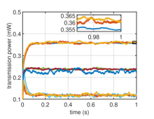
Figure 3: Gradient-play dynamics (6) subject to disturbances
Refer to caption
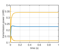
Figure 4: Agent dynamics ΣisubscriptΣ𝑖\Sigma_{i} (23) subject to disturbances
Refer to caption
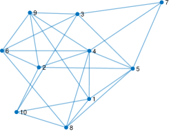
Figure 5: Random communication graph, Gcsubscript𝐺𝑐G_{c}, λ2=2.6158subscript𝜆22.6158\lambda_{2}=2.6158

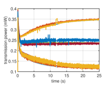
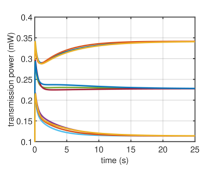
First, we consider that each agent has full information about the others’ actions and we compare the results of agent dynamics, (23), with a standard gradient-play scheme (6). As seen in Fig. 3 and Fig. 4, (6) do not the reject disturbances (sustained fluctuations in the OSNR values), while (23) successfully reject disturbances and converge to the NE found in [39]. Next, assume each agent has partial information over a random graph, Gcsubscript𝐺𝑐G_{c}, Fig. 5. The results of dynamics (16) are plotted in Fig. 7, while those of the Laplacian-based gradient dynamics (7) are shown in Fig. 6, with similar comparison.
Refer to caption
Figure 6: Laplacian-based dynamics (7) over Gcsubscript𝐺𝑐\!G_{c}\!
Refer to caption
Figure 7: Agent dynamics ΣisubscriptΣ𝑖\!\Sigma_{i}\! (16) subject to disturbances over Gcsubscript𝐺𝑐\!G_{c}\!

VI-B Sensor Networks

Our next example is similar to the one investigated in [14]. However, our algorithm uses a continuous-time gradient-play inspired feedback instead of the discrete-time extremum seeking algorithm used in [14]. It is also important to note that while [14] considers noisy feedbacks, it does not consider disturbance rejection as we have posed it here.

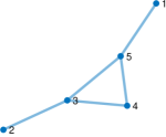
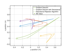
Consider a group of five mobile robots in the plane in a sensor network. Each agent has a cost function that is a function of all robots’ positions, (xi,xi)subscript𝑥𝑖subscript𝑥𝑖(x_{i},x_{-i}),

Ji(xi,xi)=xiTxi+xiTri+jxixj2subscript𝐽𝑖subscript𝑥𝑖subscript𝑥𝑖superscriptsubscript𝑥𝑖𝑇subscript𝑥𝑖superscriptsubscript𝑥𝑖𝑇subscript𝑟𝑖subscript𝑗superscriptnormsubscript𝑥𝑖subscript𝑥𝑗2\displaystyle J_{i}(x_{i},x_{-i})=x_{i}^{T}x_{i}+x_{i}^{T}r_{i}+\sum_{j\in\mathcal{I}}\|x_{i}-x_{j}\|^{2} (36)

where r1=col(2,2)subscript𝑟1col22r_{1}\!=\!\operatorname{col}(2,-2), r2=col(2,2)subscript𝑟2col22r_{2}\!=\!\operatorname{col}(-2,-2), r3=col(4,2)subscript𝑟3col42r_{3}\!=\!\operatorname{col}(-4,2), r4=col(2,4)subscript𝑟4col24r_{4}\!=\!\operatorname{col}(2,-4), and r5=col(3,3)subscript𝑟5col33r_{5}\!=\!\operatorname{col}(3,3). We consider two types, velocity actuated and force-actuated robots, and in each case we consider the full-information and the partial-information case with communication over a random graph, Gcsubscript𝐺𝑐G_{c} (Fig. LABEL:fig:Gc11).

Refer to caption
Figure 8: Random Communication Graph, Gcsubscript𝐺𝑐G_{c}

VI-B1 Velocity-Actuated Robots

Consider that each agent in the network is a velocity-actuated robot with dynamics given by (14), where di=col(0.5,0)subscript𝑑𝑖col0.50d_{i}=\operatorname{col}(0.5,0) is a constant disturbance.

Refer to caption
Figure 9: Comparison of (23) and (6) for single-integrator agents

We consider first that each agent has full information about the other’s actions and compare our algorithm (23) to the standard gradient-play (6). In Fig. 9 solid-lines depict gradient-play results in the disturbance-free case. In the presence of disturbances, as seen in Fig. 9, (23) (dashed-lines) converges to the same NE values, while the standard gradient-play (dotted-lines) does not.
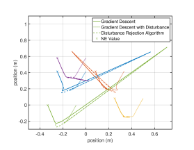
Refer to caption
Figure 10: Comparison of (16) &\& (7) for single-integrator agents

Next consider that each agent only has partial-information communicated over a graph, Gcsubscript𝐺𝑐G_{c}. We compare our algorithm (16) to that of the Laplacian based-gradient dynamics (7) in Fig. 10, where solid-lines depict (7) results in the disturbance-free case. In the presence of disturbances, Fig. 10 shows that (16) (dashed-lines) converges to the same NE values as found by the full-information case, Fig. 9, while (7) (dotted-lines) does not.

VI-B2 Force-Actuated Robots

Consider that each agent is modelled as double integrator, (24) where di=col(0.5,0)subscript𝑑𝑖col0.50d_{i}=\operatorname{col}(0.5,0). The corresponding results are shown in Fig. 11 (full information case) and Fig. 12 (partial-information over Gcsubscript𝐺𝑐G_{c}), where dashed-lines correspond to (34) and (28), respectively, while dotted-lines to the disturbance-free learning algorithm.
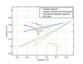
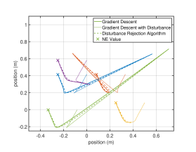
Refer to caption
Figure 11: Results of (34) for double-integrator agents
Refer to caption
Figure 12: Results of (28) for double-integrator agents
Remark 7

Although we did not specifically investigate systems with noisy feedbacks, it is possible to show that due to their ISS properties, the dynamics (16) and (28) have a certain amount of robustness to feedback noise, such as the type investigated in [14] and [16]. The ISS property implies that for any bounded feedback noise, the steady-state solution will remain in a neighbourhood of the NE.

VII Conclusions

We considered Nash equilibrium seeking schemes for (multi)-integrator agents subject to external disturbances. We addressed the case of full information on the others’ decisions, as well as the case where agents have partial-decision information, based on local observation and communication. In both cases, we proposed new continuous-time dynamic schemes that converge to the Nash equilibrium, irrespective of the disturbance. Besides a gradient-play component, the proposed agent dynamics have a dynamic internal-model component, and, in the case of partial-information, a consensus component that drives agents to reach the decision-estimate consensus subspace.

References

  • [1] X. Fan, T. Alpan, M. Arcak, T. Wen, and T. Başar, “A passivity approach to game-theoretic CDMA power control,” Automatica, vol. 42, pp. 1837–1847, 2006.
  • [2] H. Li and Z. Han, “Competitive spectrum access in cognitive radio networks: Graphical game and learning,” in Proc. of the 2010 IEEE WCNC, Apr. 2010, pp. 1–6.
  • [3] X. Chen and J. Huang, “Spatial spectrum access game: Nash equilibria and distributed learning,” in Proc. of the 13th ACM MobiHoc, Jun. 2012, pp. 205–214.
  • [4] L. Pavel, Game Theory for Control of Optical Networks, 3rd ed., ser. Static & Dynamic Game Theory: Foundations & Applications.   Birkhäuser-Springer Science, 2012.
  • [5] ——, “A noncooperative game approach to OSNR optimization in optical networks,” IEEE Trans. Autom. Control, vol. 51, no. 5, pp. 848–852, May 2006.
  • [6] A.-H. Mohsenian-Rad, V. W. Wong, J. Jatskevich, R. Schober, and A. Leon-Garcia, “Autonomous demand-side management based on game-theoretic energy consumption scheduling for the future smart grid,” IEEE Trans. Smart Grid, vol. 1, no. 3, pp. 320–331, Dec. 2010.
  • [7] S. Grammatico, “Exponentially convergent decentralized charging control for large populations of plug-in electric vehicles,” in Proc. of the 55th IEEE CDC, Dec. 2016, pp. 5775–5780.
  • [8] H. Ito, “Disturbance and delay robustness guarantees of gradient systems based on static noncooperative games with an application to feedback control for PEV charging load allocation,” IEEE Trans. Control Syst. Technol., vol. 21, no. 4, pp. 1374–1385, Jul. 2013.
  • [9] H. Yin, U. V. Shanbhag, and P. G. Mehta, “Nash equilibrium problems with scaled congestion costs and shared constraints,” IEEE Trans. Autom. Control, vol. 56, no. 7, pp. 1702–1708, Jul. 2011.
  • [10] T. Alpcan and T. Başar, Distributed Algorithms for Nash Equilibria of Flow Control Games.   Birkhäuser Boston, 2005.
  • [11] W. Lin, Z. Qu, and M. A. Simaan, “Distributed game strategy design with application to multi-agent formation control,” in Proc. of the 53rd IEEE CDC, Dec. 2014, pp. 433–438.
  • [12] P. Frihauf, M. Krstic, and T. Başar, “Nash Equilibrium Seeking in Noncooperative Games,” IEEE Trans. on Automatic Control, vol. 57, no. 5, pp. 1192–1207, 2012.
  • [13] Y. Taing and L. Pavel, “An EDFA Hsubscript𝐻H_{\infty} controller for suppression of power excursions due to pilot tones and network traffic,” IEEE Photon. Technol. Lett., vol. 18, no. 18, pp. 1916–1918, Sep. 2006.
  • [14] M. S. Stankovic, K. H. Johansson, and D. M. Stipanonic, “Distributed seeking of Nash equilibria with application to mobile sensor networks,” IEEE Trans. Autom. Control, vol. 57, no. 4, pp. 904–919, Apr. 2012.
  • [15] M. Zhu and S. Martinez, “Distributed coverage games for energy-aware mobile sensor networks,” SIAM J. Control Optim., vol. 51, no. 1, pp. 1–27, 2013.
  • [16] P. Mertikopoulos and M. Staudigl, “Convergence to Nash equilibrium in continuous games with noisy first-order feedback,” in Proc. of the 56th IEEE CDC, Dec. 2017, pp. 5609–5614.
  • [17] Z. Deng and S. Liang, “Distributed algorithms for aggregative games of multiple heterogeneous Euler-Lagrange systems,” Automatica, vol. 99, pp. 246–252, 2019.
  • [18] M. Bürger and C. D. Persis, “Dynamic coupling design for nonlinear output agreement and time-varying flow control,” Automatica, vol. 51, pp. 210–222, 2015.
  • [19] C. D. Persis and B. Jayawardhana, “On the internal model principle in the coordination of nonlinear systems,” IEEE Trans. Control Netw. Syst., vol. 1, no. 3, pp. 272–282, Sep. 2015.
  • [20] Z. Ding, “Consensus output regulation of a class of heterogeneous nonlinear systems,” IEEE Trans. Autom. Control, vol. 49, no. 12, pp. 2244–2247, Dec. 2004.
  • [21] D. Xu, X. Wang, Y. Hong, and Z.-P. Jiang, “Global robust distributed output consensus of multi-agent nonlinear systems: An internal model approach,” Systems & Control Letters, vol. 87, pp. 64–69, 2016.
  • [22] J. Xiang and Y. L. ad David J. Hill, “Cooperative output regulation of linear multi-agent network systems with dynamic edges,” Automatica, vol. 77, pp. 1–13, 2017.
  • [23] X. Wang, P. Yi, and Y. Hong, “Dynamic optimization for multi-agent systems with external disturbances,” Control Theory Tech, vol. 12, no. 2, pp. 132–138, May 2014.
  • [24] X. Wang, Y. Hong, and H. Ji, “Distributed optimization for a class of nonlinear multiagent systems with disturbance rejection,” IEEE Trans. Cybern., vol. 46, no. 7, pp. 1655–1666, Jul. 2016.
  • [25] N.-T. Trand, Y.-W. Wang, and W. Yang, “Distributed optimization problem for double-integrator systems with the presence of the exogenous disturbance,” Neurocomputing, vol. 272, pp. 386–395, Jan. 2018.
  • [26] D. Mateos-Nunes and J. Cortes, “Noise-to-state exponentially stable distributed convex optimization on weight-balanced digraph,” SIAM J. Control Optim., vol. 54, no. 1, pp. 266–290, 2016.
  • [27] D. Gadjov and L. Pavel, “A passivity-based approach to nash equilibrium seeking over networks,” IEEE Transactions on Automatic Control, vol. 64, no. 3, pp. 1077–1092, 2019.
  • [28] A. Romano and L. Pavel, “Dynamic gradient play for NE seeking with disturbance rejection,” in Proc. of 57th IEEE CDC, Dec. 2018, pp. 346–351.
  • [29] H. K. Khalil, Nonlinear Systems, 3rd ed.   Princeton Hall, 2002.
  • [30] C. Godsil and G. Royle, Algebraic Graph Theory, ser. Graduate Texts in Mathematics.   Springer New York, 2001.
  • [31] G. Scutari, F. Facchinei, J.-S. Pang, and D. P. Pallomar, “Real and complex monotone communication games,” IEEE Trans. Inf. Theory, vol. 60, no. 7, pp. 400–409, Jul. 2014.
  • [32] S. Flåm, “Equilibrium, evolutionary stability and gradient dynamics,” International Game Theory Review, vol. 4, no. 04, pp. 357–370, 2002.
  • [33] A. Isidori and C. I. Byrnes, “Output regulation of nonlinear systems,” IEEE Trans. Autom. Control, vol. 35, no. 2, pp. 131–140, Feb. 1990.
  • [34] A. Isidori, Nonlinear Control Systems, 3rd ed., ser. Communication and Control Engineering.   Springer, 1995.
  • [35] L. Marconi and A. Isidori, A Unifying Approach to the Design of Nonlinear Output Regulators.   Springer-Verlag, 2007.
  • [36] X. G. H. Attouch and P. Redont, “The heavy ball with friction method, i. the continuous dynamical system: Global exploration of the local minima of a real-valued function by asymptotic analysis of a dissipative dynamical system,” Comm. in Contemporary Mathematics, vol. 2, no. 1, pp. 1–34, 2000.
  • [37] F. Alvarez, “On the minimizing property of a second order dissipative system in Hilbert spaces,” SIAM J. Control. Optim., vol. 38, no. 4, pp. 1102–1119, 2000.
  • [38] Y. Pan and L. Pavel, “Games with coupled propogated contraints in optical networks with multi-link topologies,” Automatica, vol. 45, pp. 871–880, 2009.
  • [39] F. Salehisadaghiani and L. Pavel, “Distributed Nash equilibrium seeking: A gossip-based algorithm,” Automatica, vol. 72, pp. 209–216, 2016.