Exceptional point enhances sensitivity of optomechanical mass sensors

Abstract

We propose an efficient optomechanical mass sensor operating at exceptional points (EPs), non-hermitian degeneracies where eigenvalues of a system and their corresponding eigenvectors simultaneously coalesce. The benchmark system consists of two optomechanical cavities (OMCs) that are mechanically coupled, where we engineer mechanical gain (loss) by driving the cavity with a blue (red) detuned laser. The system features EP at the gain and loss balance, where any perturbation induces a frequency splitting that scales as the square-root of the perturbation strength, resulting in a giant sensitivity factor enhancement compared to the conventional optomechanical sensors. For non-degenerated mechanical resonators, quadratic optomechanical coupling is used to tune the mismatch frequency in order to get closer to the EP, extending the efficiency of our sensing scheme to mismatched resonators. This work paves the way towards new levels of sensitivity for optomechanical sensors, which could find applications in many other fields including nanoparticles detection, precision measurement, and quantum metrology.

I Introduction

Owing to a rapid progress in micro/nano-engineering of mechanical resonators, tremendous advances have been made in mass sensing in the view of achieving ultra sensitive detection [1] ; [2] . Resonant mass sensors are widely used in diverse fields of science and technologies. For instance, they are actively used to detect single biomolecules, viruses, nanoparticles and others nano-objects. Because of these interesting applications, nano-mechanical mass sensors have deserved much attention over the last few years. This has led to detections ranging from femtogram ($10^{-15}\rm{g}$) [3] though attogram ($10^{-18}\rm{g}$) [4] and zeptogram ($10^{-21}\rm{g}$) [5] to yoctogram ($10^{-24}\rm{g}$) [6] .

Besides these sensors based on electrical excitations, all-optical mass sensors have been proposed as well, with the aim of reaching new levels of sensitivity and to breakthrough the limitation of frequency restriction (see [7] and the references therein). Optomechanical sensors, have been revealed as excellent candidates for mass detection due to their simplicity, sensitivity and because the optical field serves both as an actuator and a probe for precise monitoring of the mechanical frequencies. Single optomechanical sensors, exploiting nonlinearies of the systems, were proposed in [8] ; [9] ; [10] whereas coupled optomechanical cavities have been used for sensing in [11] ; [12] . A mechanical resonator was inserted inside one of the coupled optical cavities in [11] , while a hybrid opto-electromechanical system consisting of an optical and microwave cavities coupled to a common mechanical oscillator has been used in [12] . It resulted that sensors based on coupled systems perform better than their counterpart that are based on single cavity. This conclusion remains the same even for coupled mechanical resonators driving by a common electromagnetic field as shown in [13] ; [14] . The main reason of such performance lies on the fact that, sensitivity in coupled structures is determined through the splitting of eigenmodes, and it therefore can be significantly increased even without entering the strong coupling regime. This is not the case neither for electromechanical nor single optomechanical mass sensors aforementioned, where the sensing process employs tracking the frequency shifts of the mechanical resonator due to mass changes induced by any added tiny object [1] ; [2] . Moreover, simple multimodal response of a mechanical resonator enables mass sensing at much higher levels of accuracy than what is typically achieved with a single frequency shift measurement [15] . It goes without saying that mass sensor performances are enhanced in coupled systems that feature strong coupling regime or those exhibiting very narrow splitting in their eigenmodes structure.

Recently, sensitivity enhancement of more than threefold in particles detection has been theoretically demonstrated with a sensor operating at exceptional points (EPs) [16] . Owing to the complex square-root topology near an EP, any perturbation lifts the degeneracy leading to a frequency splitting that scales as the square-root of the perturbation strength. This splitting is therefore larger for sufficiently small perturbation than the splitting observed in conventional sensing schemes, where the linewidth or frequency shift/splitting is proportional to the strength of the perturbation. Later on, these theoretical results have been validated by two experimental works, at EP in whispering-gallery-mode micro-toroid cavity [17] and with higher order EP in parity-time ($\mathcal{PT}$)-symmetric photonic laser molecule [18] . Along the same line, the performance of cavity-assisted metrology, where a cavity is coupled to the device under test, has been enhanced near EP in $\mathcal{PT}$-symmetric micro-cavities [19] . It follows that EP is a useful tool for next generation of sensors in reaching new levels of sensitivity.

Our proposal is based on two optomechanical cavities, mechanically coupled through their moving mechanical resonators. This benchmark system has an advantage that it enables to get an effective coupled mechanical system, where mechanical gain (loss) can be easily engineered by driving the cavity with a blue (red) detuned laser. At the balance between gain and loss, the system features EP in its mechanical spectrum [20] , which is the key point of our optomechanical mass sensor-based EP. The proposed sensor differs from those known [16] ; [17] ; [18] ; [19] on at least three points: (i) it operates at an EP generated on its mechanical spectrum (instead of the optical spectrum), (ii) the gain and loss are self-engineered while the cavities are driven, and (iii) it does not needs the $\mathcal{PT}$-symmetric requirement. At the vicinity of EP, our proposed sensing scheme has shown a giant enhancement sensitivity factor compared to conventional opto-(electro)mechanical sensing schemes. This efficiency comes from topological complex square-root near the EP, and is highly pronouced for small perturbations. Bearing in mind the laborious micro/nanofabrication task of engineering two identical mechanical resonators, we have extended our results to non-degenerated mechanical resonators, where their frequency mismatch can be tuned through quadratic coupling that is well known in optomechanics [21] . This work is organized as follows. In Sec. II, the model and its dynamical equations up to the EP features are described. The sensitivity enhancement, at the vicinity of EP for degenerated mechanical resonators, is presented in Sec. III. Section IV is devoted to the sensitivity assisted by quadratic coupling for the non-degenerated case, while Sec. V concludes the work.

II Modelling and dynamical equations

The system of our proposal is the one sketched in Fig. 1a. It consists of two optomechanical cavities, mechanically coupled through their moving mechanical resonators. The first cavity is driven with a red-detuned laser while the second one is excited with a blue-detuned driving field. By symmetrically driving the cavities at the mentioned sidebands, we can engineer either mechanical gain or loss. In the rotating frame of the driving fields ($\omega_{p}$), the Hamiltonian ($\hbar=1$) describing this system is,

$$H=H_{OM}+H_{int}+H_{drive},$$ (1)

with

$$\left\{\begin{array}[c]{c}H_{OM}=\sum_{j=1,2}\omega_{j}b_{j}^{{\dagger}}b_{j}-\Delta_{j}a_{j}^{{\dagger}}a_{j}\\ -ga_{j}^{{\dagger}}a_{j}(b_{j}^{{\dagger}}+b_{j})\\ H_{int}=-J(b_{1}b_{2}^{{\dagger}}+b_{1}^{{\dagger}}b_{2})\\ H_{drive}=E(a^{{\dagger}}+a).\end{array}\right.$$ (2)

In this Hamiltonian, $a_{j}$ and $b_{j}$ are the annihilation bosonic field operators describing the optical and mechanical resonators, respectively. The mechanical displacements $x_{j}$ are connected to $b_{j}$ as $x_{j}=x_{{}_{\rm{ZPF}}}(b_{j}+b_{j}^{{\dagger}})$, where $x_{{}_{\rm{ZPF}}}$ is the zero-point fluctuation amplitude of the mechanical resonator. The mechanical frequency of the $j^{th}$ resonator is $\omega_{j}$ and $\Delta_{j}=\omega_{p}^{j}-\omega_{cav}^{j}$ is the optical detuning between the optical and the cavity ($\omega_{cav}^{j}$) frequencies . The mechanical coupling strength between the two mechanical resonators is $J$, and the linear optomechanical coupling is $g$. By setting the mean values of the operators, $\langle a\rangle=\alpha_{j}$ for the optics and $\langle b\rangle=\beta_{j}$ for the mechanics, one can derive the following classical set of nonlinear equations of our system,

$$\left\{\begin{array}[]{c}\dot{\alpha}_{j}=[i(\Delta_{j}+g(\beta_{j}^{\ast}+\beta_{j}))-\frac{\kappa}{2}]\alpha_{j}-i\sqrt{\kappa}\alpha^{\rm{in}},\\ \dot{\beta}_{j}=-(i\omega_{j}+\frac{\gamma_{m}}{2})\beta_{j}+iJ\beta_{3-j}+ig\alpha_{j}^{\ast}\alpha_{j},\end{array}\right.$$ (3)

where optical ($\kappa$) and mechanical ($\gamma$) dissipations have been added, and the amplitude of the driving pump has been substituted as $E=\sqrt{\kappa}\alpha^{\rm{in}}$ in order to account for losses. In this form, the input laser power $\rm{P_{in}}$ acts through $\alpha^{\rm{in}}=\sqrt{\frac{\rm{P_{in}}}{\hbar\omega_{p}}}$. Without loss of generality, the parameters $\gamma_{m}$, $g$, and $\kappa$ are assumed to be degenerated for the whole system. Moreover, they follows the hierarchy $\gamma_{m},g\ll\kappa\ll\omega_{m}$, as encountered in resolved sideband regime experiments [22] ; [23] .

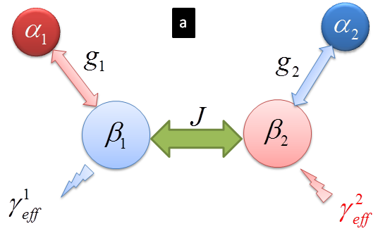
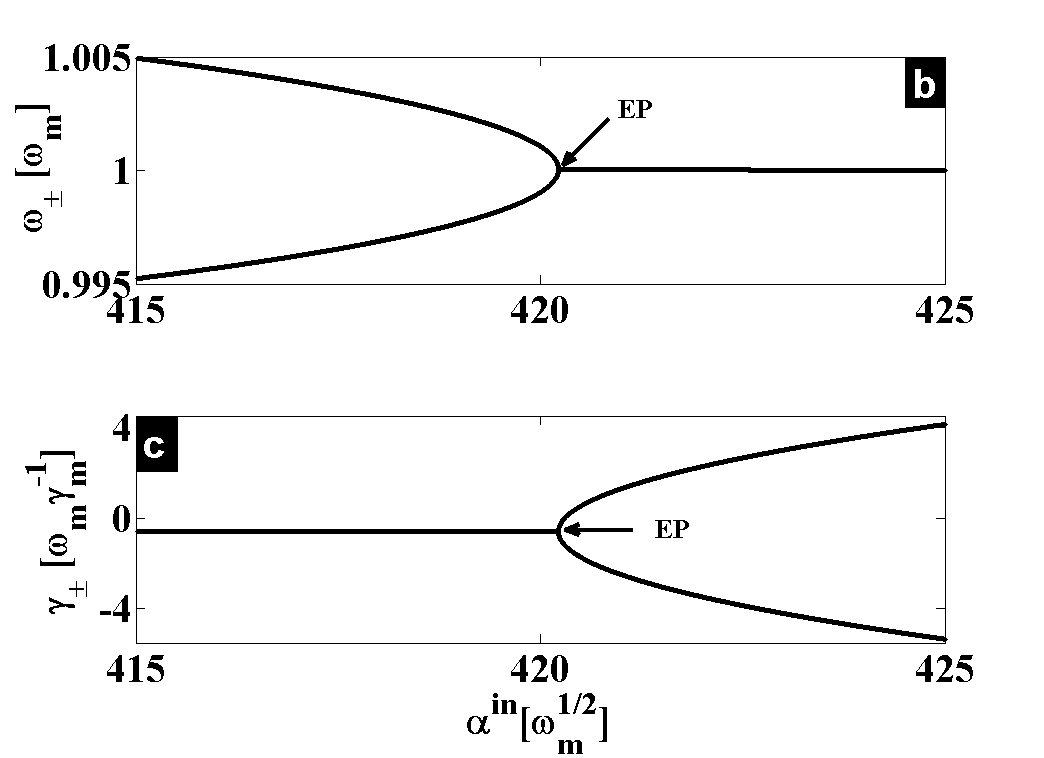
Figure 1: (a) Generic setup. Two optomechanical cavities, one with gain and the other generating losses are mechanically coupled. (b)-(c) Real and imaginary parts of the eigenvalues versus the driving strength $\alpha^{in}$, which depict the EP feature.

To investigate sensitivity performance of our proposed sensor, we need to compute the eigenvalues of the effective mechanical system in order to identify the EP feature. One can obtain this effective system by integrating $\alpha_{j}(t)$ out of the full set of Eq. (3). This can be straightforwardly done by approaching the mechanical oscillations with the ansatz, $\beta_{j}(t)=\bar{\beta}_{j}+A_{j}\exp(-i\omega_{{}_{\rm{lock}}}t)$ (see more details in [20] ). $\bar{\beta}_{j}$ is a constant shift in the origin of the movement, $A_{j}$ is the slowly time dependent amplitude, and $\omega_{{}_{\rm{lock}}}$ is the mechanical degenerated frequency when the resonators experience frequency locking phenomenon. This leads to the following mechanical effective Hamiltonian,

$$H_{\rm{eff}}=\begin{bmatrix}\omega_{\rm{eff}}^{1}-i\frac{\gamma_{\rm{eff}}^{1}}{2}&-J\\ -J&\omega_{\rm{eff}}^{2}-i\frac{\gamma_{\rm{eff}}^{2}}{2}\end{bmatrix},$$ (4)

having the eigenvalues

$$\lambda_{\pm}=\frac{\omega_{\rm{eff}}^{1}+\omega_{\rm{eff}}^{2}}{2}-\frac{i}{4}\left(\gamma_{\rm{eff}}^{1}+\gamma_{\rm{eff}}^{2}\right)\pm\frac{\sigma}{4},$$ (5)

with

$$\sigma=\sqrt{16J^{2}+[2(\omega_{eff}^{1}-\omega_{eff}^{2})+i(\gamma_{eff}^{2}-\gamma_{eff}^{1})]^{2}}.$$ (6)

Here, $\omega_{\rm{eff}}^{j}=\omega_{m}+\delta\omega_{opt}^{j}$ and $\gamma_{\rm{eff}}^{j}=\gamma_{m}+\gamma_{\rm{opt}}^{j}$ are the effective frequencies and dampings, respectively. Furthermore, the quantities $\delta\omega_{opt}^{j}$ and $\gamma_{\rm{opt}}^{j}$ are the optical spring effect and optical damping induced by the optical fields, respectively. These terms are given as,

$$\delta\omega_{opt}^{j}=-\frac{2\kappa(g\alpha^{in})^{2}}{\omega_{lock}\epsilon_{j}}\rm{Re}\left(\sum_{n}\frac{J_{n+1}\left(-\epsilon_{j}\right)J_{n}\left(-\epsilon_{j}\right)}{h_{n+1}^{j\ast}h_{n}^{j}}\right),$$ (7)

and

$$\gamma_{\rm{opt}}^{j}=\frac{2(g\kappa\alpha^{\rm{in}})^{2}}{\epsilon_{j}}\sum_{n}\frac{J_{n+1}\left(-\epsilon_{j}\right)J_{n}\left(-\epsilon_{j}\right)}{\left|h_{n+1}^{j\ast}h_{n}^{j}\right|^{2}},$$ (8)

where $\epsilon_{j}=\frac{2g\rm{Re}(A_{j})}{\omega_{{}_{\rm{lock}}}}$ is a normalized amplitude, $J_{n}$ the Bessel function, $h_{n}^{j}=i\left(n\omega_{{}_{\rm{lock}}}-\tilde{\Delta}_{j}\right)+\frac{\kappa}{2}$, and $\tilde{\Delta}_{j}=\Delta_{j}+2g(\bar{\beta}_{j})$ the effective detuning [20] . The eigenfrequencies and the dampings of the system are defined as the real [$\omega_{\pm}=\rm{Re}(\lambda_{\pm})$] and imaginary [$\gamma_{\pm}=\rm{Im}(\lambda_{\pm})$] parts of $\lambda_{\pm}$, respectively.

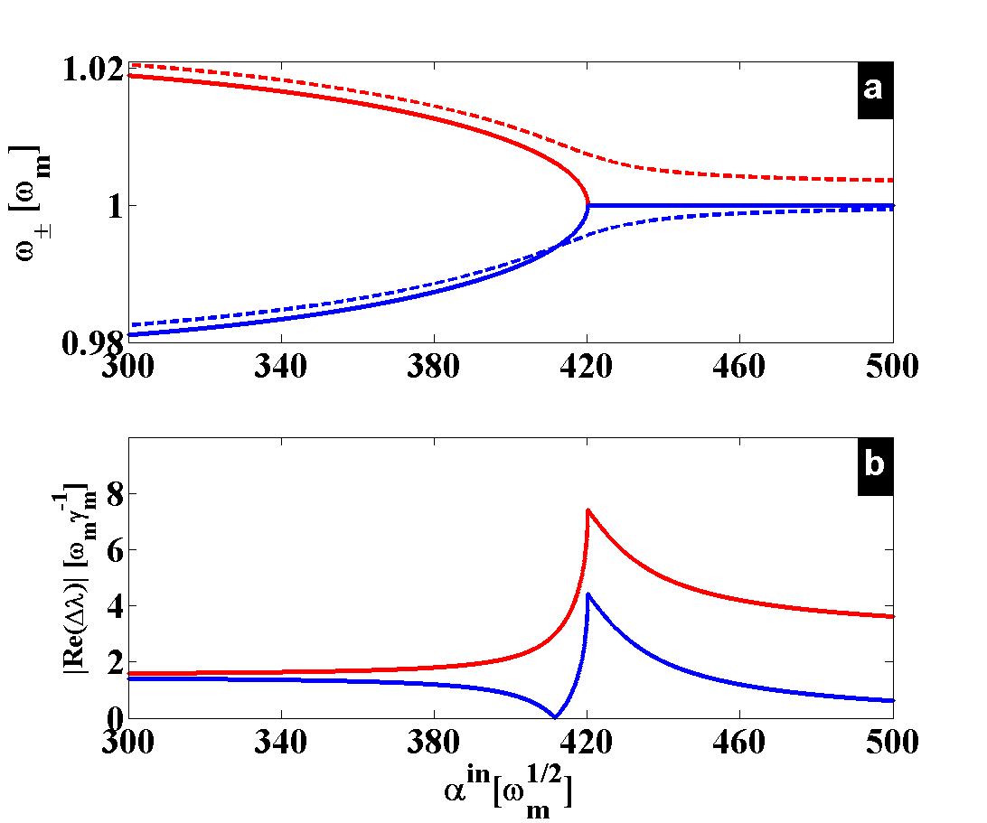
Figure 2: (a) Frequencies of the effective mechanical system, before perturbation (full lines) and after perturbation by a mass deposition (dashed lines). (b) Gap difference between the perturbed and reference frequencies shown in (a). These quantities are plotted versus the driving strength $\alpha^{in}$. Note the difference in the units on the $y$-axis in (a) and (b).

At the EP, both these pairs of frequencies and dampings coalesce, $\omega_{-}=\omega_{+}\equiv\omega_{lock}$ and $\gamma_{-}=\gamma_{+}$. From Eq. (5), this is equivalent to $\sigma=0$, which requires both control of real and imaginary parts of $\sigma$, through the driving fields ($\alpha^{in}_{j}$) and detunings ($\Delta_{j}$) [24] . For a proof of concept of the proposed sensor, we assume in the next section that the two mechanical resonators are degenerated ($\omega_{j}\equiv\omega_{m}$). However, the non-degenerated case, where there is a mismatch frequency due to micro/nanofabrication imperfections for intance, is later on discussed in section Sec. IV.

III Sensitivity at the exceptional point

The eigenvalues of our effective mechanical system undergo a singularity (known as EP) in their spectrum as shown in Fig. 1(b)-(c). The efficiency of the proposed sensor depends on this EP, which emerges from the eigenvalues given in Eq. (5), instead of tracking the resonant frequency shift induced by mass deposition on the surface of the resonators [8] ; [9] ; [10] ; [11] ; [12] ; [13] . For ordinary mass sensor, the relationship between the frequency shift $\delta\omega$ with the deposited mass $\delta m$ is given by [1] ; [2] ,

$$\delta m=\frac{2m}{\omega_{m}}\delta\omega=\mathcal{R}^{-1}\delta\omega,$$ (9)

where $\mathcal{R}=\tfrac{\omega_{m}}{2m}$ stands for the mass responsivity and $m$ is the mass of the resonator supporting the deposition. It results that the induced frequency shift is proportional to the strength of the perturbation. At the EP, both frequencies ($\omega_{\pm}$) and dampings ($\gamma_{\pm}$) coalesce (see Fig. 1b), and any external perturbation will split these eigenvalues leading to high sensitivity (see Fig. 3). To get insight of this feature, we assume that a mass deposition has landed on the mechanical resonator driven by the blue-detuned field ($m_{2}\equiv m$), which will induce its resonance to shift according to Eq. (9). As the resonators are coupled, this localized shift will affect the whole system, resulting in a splitting at the EP. For degenerated resonators, and for weak driving regime one has $\delta\omega_{opt}^{j}\ll\omega_{m}$, and Eq. (5) simplifies to

$$\lambda_{\pm}\approx\omega_{m}-\frac{i}{4}\left(\gamma_{\rm{eff}}^{1}+\gamma_{\rm{eff}}^{2}\right)\pm\sqrt{J^{2}-\left(\frac{\Delta\gamma_{eff}}{4}\right)^{2}},$$ (10)

with $\Delta\gamma_{eff}=\gamma_{eff}^{2}-\gamma_{eff}^{1}$. As the second resonator experiences a small perturbation $\delta m$ (or shift $\delta\omega$), this affects the eigenvalues as (see appendix A),

$$\begin{split}\lambda_{\pm}^{\delta\omega}&\approx\omega_{m}+\frac{\delta\omega}{2}-\frac{i}{4}\left(\gamma_{\rm{eff}}^{1}+\gamma_{\rm{eff}}^{2}\right)\\ &\pm\sqrt{J^{2}-\left(\frac{\Delta\gamma_{eff}}{4}\right)^{2}+\frac{\delta\omega^{2}+i\delta\omega\Delta\gamma_{eff}}{4}}.\end{split}$$ (11)

This perturbation generally affects also the optical dampings, but for the sake of a qualitative discussion and since the corresponding variations are very small (see Fig. 6(a)-(b) in appendix A), we did not include them in Eq. (11). However, it is worth noticing that these effects are fully accounted in our simulated results. We define sensitivity as the frequency shift of a supermode relative to its reference signal, i.e., the frequency splitting of these two pairs of supermodes $\rm{Re}(\Delta\lambda_{+})\equiv\rm{Re}(\lambda_{+}^{\delta\omega}-\lambda_{+})$ and $\rm{Re}(\Delta\lambda_{-})\equiv\rm{Re}(\lambda_{-}^{\delta\omega}-\lambda_{-})$ as shown in Fig. 2(a)-(b). One remarks that significant splitting is experienced at the EP (see Fig. 2(a)), resulting in a high sensitivity $|\rm{Re}(\Delta\lambda)|$ as depicted in Fig. 2(b). This feature can be approaching through our analytical investigation aforementioned. Indeed, the system undergoes the EP when $4J=\Delta\gamma_{eff}$ (see Eq. (10)). At this degeneracy point, and from Eq. (10) and Eq. (11), the splitting of the two pairs of supermodes can be deduced as (see appendix A),

$$\Delta\lambda^{EP}=\frac{1}{2}\left(\delta\omega\pm\sqrt{\delta\omega^{2}-i\delta\omega\Delta\gamma_{eff}}\right).$$ (12)

As expected, Eq. (12) shows that there is no splitting at the EP for $\delta\omega=0$. For any perturbation however ($\delta\omega\neq 0$), it reveals that the two pairs of supermodes experience different splittings $\rm{Re}(\Delta\lambda_{+})\neq\rm{Re}(\Delta\lambda_{-})$, as it appears in Fig. 2(b). This asymmetry depends on which resonator the extra mass-like perturbation has landed. By adding the deposition on the other resonator instead, we have verified that the sensitivities of the supermodes are reversed. For small enough landed mass ($|\delta\omega|\ll|\Delta\gamma_{eff}|$), both pairs of supermodes experience the same amount of splitting $\sim\sqrt{\tfrac{\delta\omega\Delta\gamma_{eff}}{8}}$ (see appendix A). It results that the splitting at the EP scales as the square-root of the strength of the perturbation $\sim\delta\omega^{1/2}$, in stark contrast with the linear dependence as it is for the conventional sensors (see Eq. (9)). Owing to this complex square-root topology near the EP, the EP-sensors perform better in detecting small mass deposition compared to the conventional ones. In this weak perturbation limit, the splitting at the EP can be expressed in terms of the deposited mass as $\sim\sqrt{\frac{\omega_{m}\delta m\Delta\gamma_{eff}}{16m}}$. From this expression and Eq. (9), we can define the sensitivity enhancement factor as,

$$\eta\equiv\left|\frac{\rm{Re}(\Delta\lambda^{\rm{EP}})}{\delta\omega}\right|=\sqrt{\frac{\Delta\gamma_{eff}}{8\delta\omega}}=\sqrt{\frac{m\Delta\gamma_{eff}}{4\omega_{m}\delta m}}.$$ (13)

which again highlights the square root dependence with $\delta m$, instead of a linear dependence, for small mass deposition. As expected, Fig. 3(a) shows the square-root-like evolution of the sensitivity versus perturbation ($\left|\rm{Re}(\Delta\lambda^{EP})\right|\propto\delta\omega^{1/2}$), which is revealed through the log-log scale representation in the inset. Hence, a $\frac{1}{2}$-slope is shown for weak perturbations, which evolves towards $1$-slope behaviour as the perturbation increases. This simply reveals the fact that, the sensitivity of EP-sensor scales linearly with the strength of the perturbations when they are large enough. This is confirmed through the enhancement factor $\eta$ depicted in Fig. 3(b), where it evolves towards the limit $\eta\sim 1$ for strong enough perturbation. It can be also seen that this factor $\eta$ is highly enhanced for weak perturbation strength (see inset), proving the efficiency of the EP-sensor in detecting small particles, mass or objects.

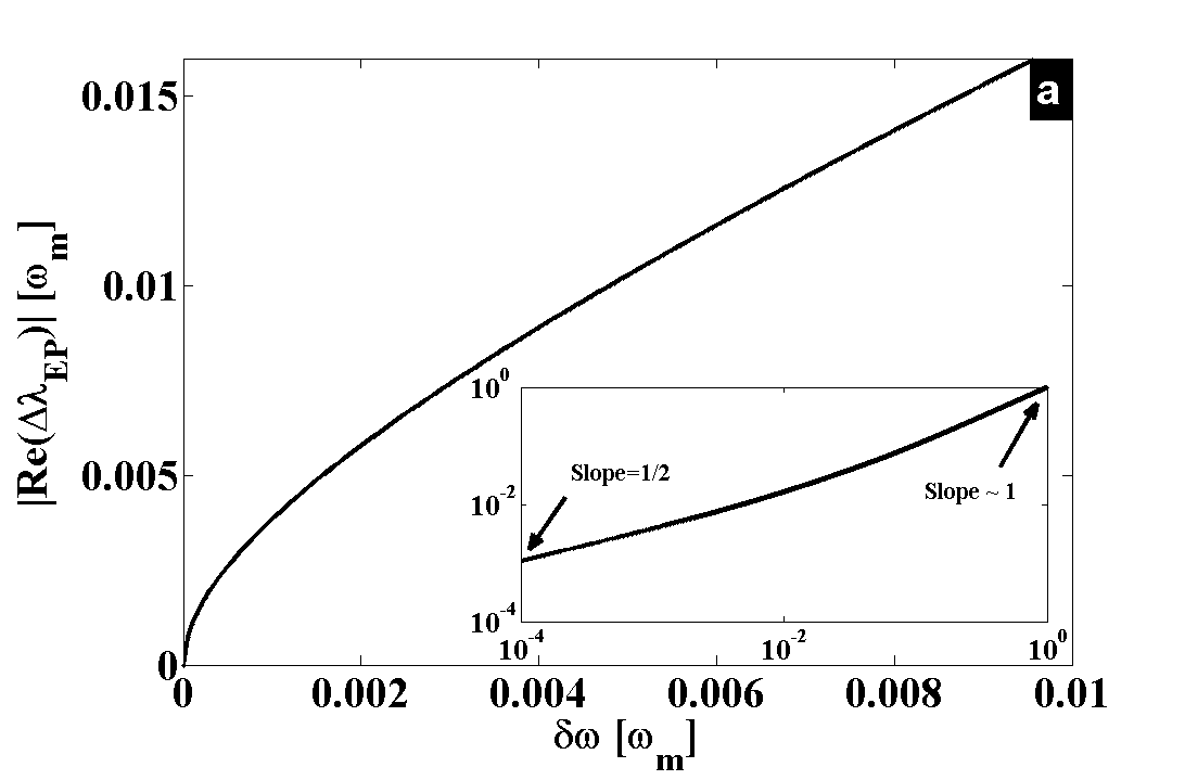
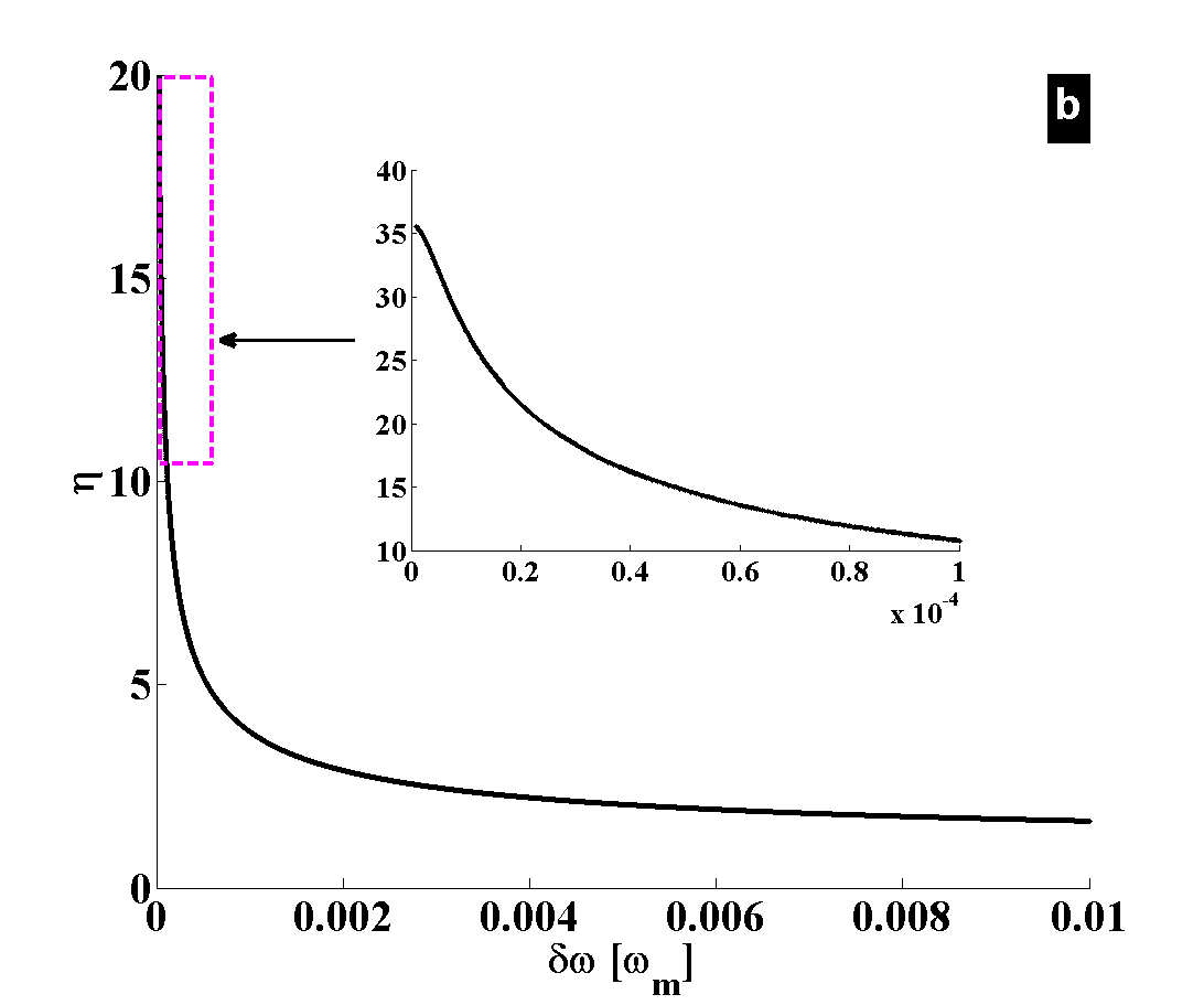
Figure 3: (a) Sensitivity at the exceptional point versus the strength of the perturbation $\delta\omega$. The inset shows the log-log scale representation. (b) Sensitivity enhancement factor $\eta$ versus $\delta\omega$. It can be seen that for weak perturbation (see inset), the EP-sensor performs better, and ends up towards the same performance as the conventional ones as the perturbation increases.

Another interesting feature of EP-sensors is that they improve their performance regarding their linewidth as well. As the linewidths are also degenerated at the EP, adding extra mass will also lift this degeneracy. This is depicted in Fig. 4(a), and the corresponding sensitivity is shown in Fig. 4(b). In contrast to Fig. 2(b), here both sensitivities given by the pairs of supermodes are the same. This can be expected by refering to the imaginary part of Eq. (12) as given in appendix A. By further driving the system, the linewidths move out of the vicinity of EP, and one of them grows whereas the other decays. This simply means that one supermode experiences gain, while the other feels loss.

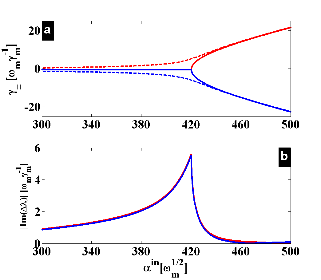
Figure 4: (a) Dampings as reference (full lines) and perturbed (dashed lines), with the associated splittings in (b). These plots are versus the driving strength $\alpha^{in}$.

IV Enhancing sensitivity through quadratic coupling

The previous section has dealt with optomechanical sensor-based EP, where the coupled mechanical resonators are degenerated. However, engineering such identical resonators is not often an obious task in micro/nano-fabrication technologies. Therefore, any mismatch between the mechanical resonance frequencies will lift the EP degeneracy, impairing the performance of the proposed sensor. It could be interesting to extend the detection process studied in the previous section to a system composed of non-degenerated resonators. This can breakthrough the limitation of micro/nano-fabrication restriction, and will pave a way towards EP-sensors which are robust against defects or fabrication imperfections. One way to go beyond this technological limitation is to engineer nonlinearities, in order to control and compensate the frequency mismatch. Such optical control of frequency has been recently investigated to enhance energy transfer between two non-degenerated mechanical resonators [25] ; [26] .

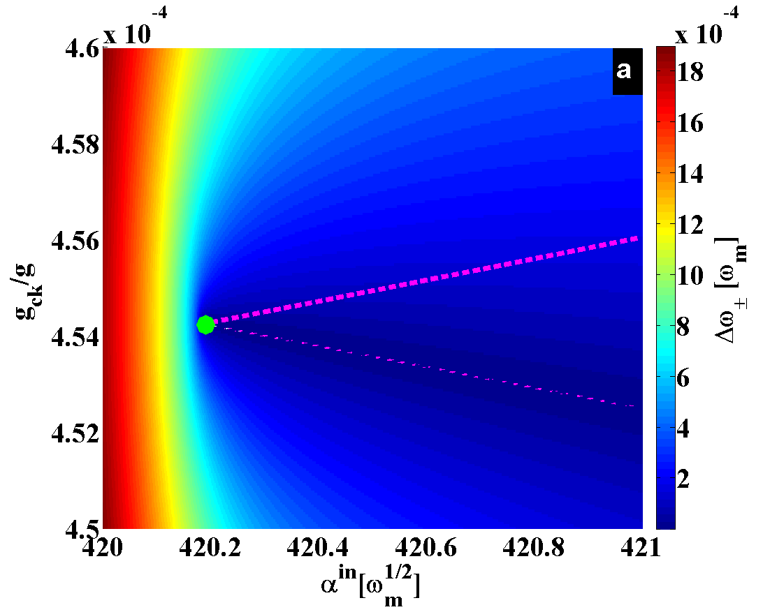
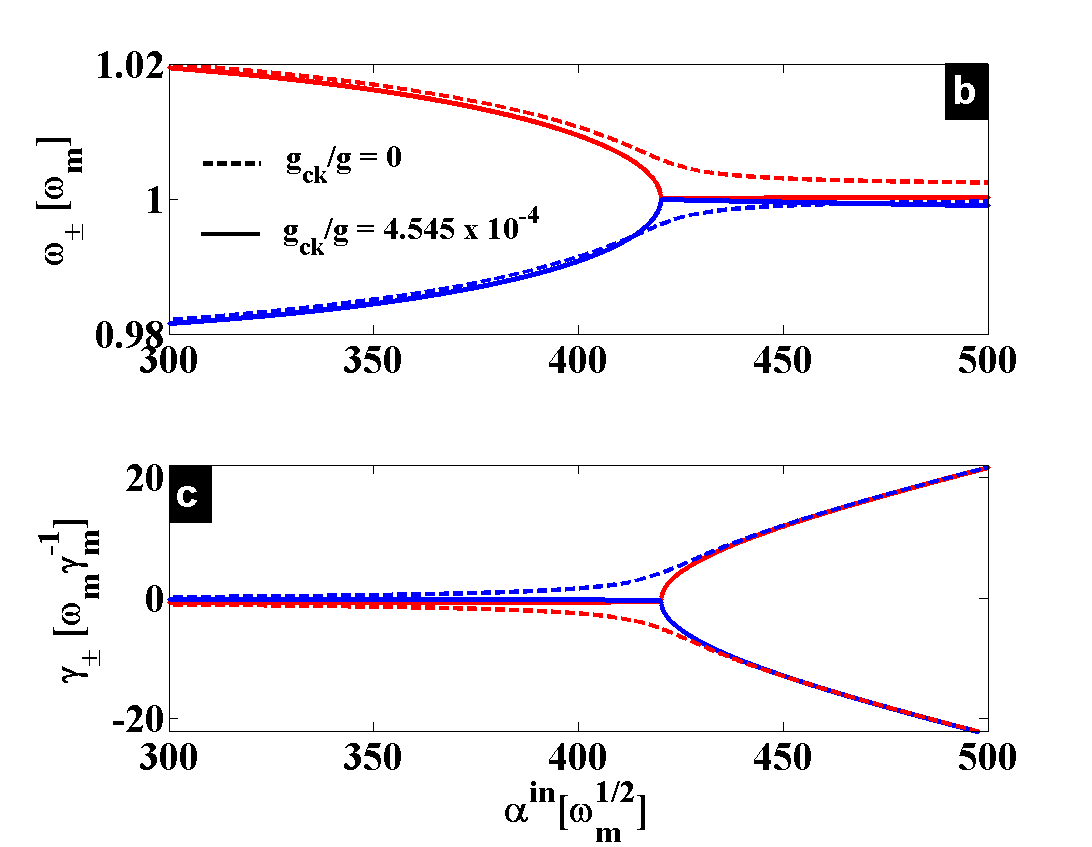
Figure 5: (a) Diagram showing the control strategy in ($\alpha^{in},g_{ck}$) space, at a fixed frequency mismatch $\nu=2\times 10^{-3}\omega_{m}$. (b),(c) Eigenvalues corresponding to the green dot in (a), where we see EP feature induced by the control strategy. The dashed lines correspond to the case without control ($g_{ck}/g=0$), whereas the control has been applied ($g_{ck}/g=4.545\times 10^{-4}$) to the solid lines.

Duffing nonlinearity has been used in [25] , whereas an optical trapping coupling was used in [26] to trap the mechanical motion. Although these technics resulted to an efficient transfer around the avoided crossing level, this was still not enough to induce EP feature in the system. The reason lies on the fact that strong coupling observed in these works leads to level repulsion, gap opening between two modes due to coupling, while EP arises from level attraction process instead [27] . To reach our goal, we propose a position-squared coupling where the optical mode is coupled in a quadratic fashion to the mechanical motion [21] . This can be engineered by optically trapping the second resonator ($\beta_{2}$) inside the cavity driven on the blue-sideband, which could have been achieved in [26] as well. The resulting cross-Kerr interaction is described by the Hamiltonian $H_{ck}=-g_{ck}a^{{\dagger}}ab^{{\dagger}}b$, which has to be accounted for Eq. (1) for a full corresponding model. After few transformations, the tuned mechanical frequency takes the form $\tilde{\omega_{2}}=\omega_{2}-g_{ck}\alpha_{2}^{\ast}\alpha_{2}$, which can be optically controlled as the cavity is driven (see appendix B). By assuming that the coupled mechanical resonators fullfill the condition $\omega_{2}>\omega_{1}$, and for a given cross-Kerr term $g_{ck}>0$, one can optically adjust the effective frequencies to satisfy $\omega_{\rm{eff}}^{1}\sim\omega_{\rm{eff}}^{2}$ that is a good requirement for EP as presented above. Therefore, cross-Kerr coupling is useful not only to engineer EP in non-degenerated coupled resonators, but it enables to enhance the performance of optomechanical sensor-based EP for mismatched set of resonators, regardless of their technological imperfections. Fig. 5(a) is a diagram showing the frequency control strategy in ($\alpha^{in},g_{ck}$) space, for a given mismatch frequency $\nu=\omega_{2}-\omega_{1}=2\times 10^{-3}\omega_{m}$. It can be seen that any mismatch ($\nu\neq 0$) requires a corresponding cross-Kerr value to reach the minimal splitting $\Delta\omega_{\pm}$ (see colorbar in Fig. 5(a)), which is depicted by the magenta dashed line for a given couple of parameters ($\alpha^{in},g_{ck}$). The eigenvalues that correspond to the green dot in Fig. 5(a) are represented in Fig. 5(b), where we can see the efficiency of the strategy control as well as the EP feature. Indeed, the dashed lines correspond to the case without control ($g_{ck}/g=0$), whereas the control has been applied ($g_{ck}/g=4.545\times 10^{-4}$) to the solid lines. The observed large splitting in the case without control simply reveals an absence of EP together with the fact that a small object can not be efficiently detected. Therefore, a position-squared coupling is a useful tool to tune non-degenerated mechanical resonators closer to their EP. Hence, detection of optomechanical sensor-based EP can be enhanced through quadratic coupling, resulting in a giant sensitivity factor compared to the conventional sensors.

V Conclusion

We have proposed an optomechanical mass sensor based on EP. The benchmark system is a mechanically coupled optomechanical system, where gain (loss) is engineered by driving the cavity with a blue (red) detuned electromagnetic field. Degeneracy known as EP shows up in the system when the gain balances losses, and any perturbation leads to a frequency splitting that scales as the square-root of the perturbation strength that greatly enhances the detection compared to the conventional optomechanical sensors. To breakthrough the limitation of micro/nanofabrication technology restriction, we have extended the performance of the proposed sensor to non-degenerated mechanical resonators by using quadratic optomechanical coupling to tune the mismatch mechanical frequency. Therefore, our sensing scheme is robust regardless of technological limitation related to the mechanical resonators ingineering, and can be applied to a versatile set of resonators. Moreover, this scheme does not require $\mathcal{PT}$-symmetric prerequisite, and can be extended to plethora of systems including, hybrid opto-electromechanical and superconducting microvawe resonators.

Appendix A Calculation details related to the sensitivity and its enhancement factor

In the main text (see Eq. (5) and Eq. (6)), we have given the eigenvalues of our effective reduced mechanical system as,

$$\lambda_{\pm}=\frac{\omega_{\rm{eff}}^{1}+\omega_{\rm{eff}}^{2}}{2}-\frac{i}{4}\left(\gamma_{\rm{eff}}^{1}+\gamma_{\rm{eff}}^{2}\right)\pm\frac{\sigma}{4},$$ (14)

with

$$\sigma=\sqrt{16J^{2}+[2(\omega_{eff}^{1}-\omega_{eff}^{2})+i(\gamma_{eff}^{2}-\gamma_{eff}^{1})]^{2}},$$ (15)

where, $\omega_{\rm{eff}}^{j}=\omega_{m}+\delta\omega_{opt}^{j}$ and $\gamma_{\rm{eff}}^{j}=\gamma_{m}+\gamma_{\rm{opt}}^{j}$ are the effective frequencies and dampings, respectively. Any perturbation ($\delta m$) of the second mechanical resonator (without loss to the generality) induces a frequency shift ($\delta\omega$) that affects the eigenvalues as,

$$\lambda_{\pm}^{\delta\omega}=\frac{\sum_{j=1,2}\omega_{\rm{j}}+\sum_{j=1,2}\delta\omega_{\rm{opt}}^{j}+\delta\omega}{2}-\frac{i}{4}\left(\gamma_{\rm{eff}}^{1}+\gamma_{\rm{eff}}^{2}\right)\pm\frac{\sigma^{\delta\omega}}{4},$$ (16)

with

$$\sigma^{\delta\omega}=\sqrt{16J^{2}+\left[2\chi+i(\gamma_{eff}^{2}-\gamma_{eff}^{1})\right]^{2}},$$ (17)

where $\chi=\left(\omega_{\rm{1}}-\omega_{\rm{2}}+\delta\omega_{\rm{opt}}^{1}-\delta\omega_{\rm{opt}}^{2}-\delta\omega\right)$, and we have localized the effect of $\delta\omega$ only on the frequencies, since it weakly affects the dampings (see Fig. 6(a)-(b)). However, the full effect is accounted in our numerical results shown in the main text. For degenerated mechanical resonators ($\omega_{j}\equiv\omega_{m}$), and in a weak driving regime ($\delta\omega_{\rm{opt}}^{j}\ll\omega_{m}$), Eq. (16) can be simplified as,

$$\begin{split}\lambda_{\pm}^{\delta\omega}&=\omega_{m}+\frac{\delta\omega}{2}-\frac{i}{4}\left(\gamma_{\rm{eff}}^{1}+\gamma_{\rm{eff}}^{2}\right)\\ &\pm\frac{1}{4}\sqrt{16J^{2}+\left[-2\delta\omega+i(\gamma_{eff}^{2}-\gamma_{eff}^{1})\right]^{2}}\\ &=\omega_{m}+\frac{\delta\omega}{2}-\frac{i}{4}\left(\gamma_{\rm{eff}}^{1}+\gamma_{\rm{eff}}^{2}\right)\\ &\pm\sqrt{J^{2}-\left(\frac{\Delta\gamma_{eff}}{4}\right)^{2}+\frac{\delta\omega^{2}-i\delta\omega\Delta\gamma_{eff}}{4}}.\end{split}$$ (18)

The sensitivity is measured by the detected change between the perturbed and the non-perturbed eigenvalues. From Eq. (18), one can deduce such quantities providing,

$$\begin{split}\lambda_{\pm}^{\delta\omega}-\lambda_{\pm}&=\frac{\delta\omega}{2}\pm\sqrt{J^{2}-\left(\frac{\Delta\gamma_{eff}}{4}\right)^{2}+\frac{\delta\omega^{2}-i\delta\omega\Delta\gamma_{eff}}{4}}\\ &\mp\sqrt{J^{2}-\left(\frac{\Delta\gamma_{eff}}{4}\right)^{2}}.\end{split}$$ (19)

As we seek to evaluate the sensitivity of our sensor at the EP where the quantity given in Eq. (19) has an optimal value, we use the condition $4J=\Delta\gamma_{eff}$ that leads to,

$$\begin{split}\lambda_{\pm}^{\rm{EP}}\equiv\left(\lambda_{\pm}^{\delta\omega}-\lambda_{\pm}\right)^{\rm{EP}}&=\frac{\delta\omega}{2}\pm\sqrt{\frac{\delta\omega^{2}-i\delta\omega\Delta\gamma_{eff}}{4}}\\ &=\frac{1}{2}\left(\delta\omega\pm\sqrt{\delta\omega^{2}-i\delta\omega\Delta\gamma_{eff}}\right).\end{split}$$ (20)

In order to ease our qualitative interpretations of the physics hidden behind Eq. (20), it is convenient to explicitly split it in real and imaginary parts. Indeed, the square-root of the complex term in Eq. (20) can be found by first converting it to polar form and then using DeMoivre’s theorem. After few calculations, we straightforwardly get,

$$\rm{Re}\left(\lambda_{\pm}^{\rm{EP}}\right)=\frac{1}{2}\left(\delta\omega\pm\sqrt{\frac{\delta\omega^{2}}{2}+\frac{\delta\omega}{2}\sqrt{\delta\omega^{2}+\Delta\gamma_{eff}^{2}}}\right),$$ (21)

and

$$\rm{Im}\left(\lambda_{\pm}^{\rm{EP}}\right)=\pm\frac{i}{2}\sqrt{\frac{\delta\omega}{2}\sqrt{\delta\omega^{2}+\Delta\gamma_{eff}^{2}}-\frac{\delta\omega^{2}}{2}}.$$ (22)

From Eqs. (21)-(22), we can straightforwardly deduce the sensitivities $\left|\rm{Re}\left(\lambda_{\pm}^{\rm{EP}}\right)\right|$ and $\left|\rm{Im}\left(\lambda_{\pm}^{\rm{EP}}\right)\right|$, which are depicted in Fig. 2(b), (or Fig. 3(a)) and Fig. 4(a), respectively. Moreover, Eq. (21) reveals that the sensitivity given by the two eigenfrequencies are not equal in general, whereas the dampings carry out the same sensitivity through Eq. (22). Furthermore, Eqs. (21)-(22) show that the sensitivity carried out through the dampings is generally less compared to the one coming from the eigenfrequencies ($\left|\rm{Im}\left(\lambda_{\pm}^{\rm{EP}}\right)\right|\leq\left|\rm{Re}\left(\lambda_{\pm}^{\rm{EP}}\right)\right|$). These qualitative explanations are revealed through Fig. 2(b) and Fig. 4(b).

In a weak perturbation limit ($|\delta\omega|\ll|\Delta\gamma_{eff}|$), Eqs. (21)-(22) are further simplified and carry out approximately the identical sensitivity through $\sim\pm\sqrt{\frac{\delta\omega\Delta\gamma_{eff}}{8}}$ and $\sim\pm i\sqrt{\frac{\delta\omega\Delta\gamma_{eff}}{8}}$, respectively. In this limit, the sensitivity enhancement factor $\eta$ yields,

$$\eta\equiv\left|\frac{\rm{Re}(\Delta\lambda_{\pm}^{\rm{EP}})}{\delta\omega}\right|=\sqrt{\frac{\Delta\gamma_{eff}}{8\delta\omega}}=\sqrt{\frac{m\Delta\gamma_{eff}}{4\omega_{m}\delta m}}.$$ (23)

For a given weak perturbation $\delta\omega=10^{-5}\omega_{m}$, Figs. 6(c)-(d) show the eigenfrequencies and their corresponding sensitivities. It can be seen that the resulted sensitivities are similar for both eigenfrequencies as expected from our analysis. We would like to underline that in the main text, we have used $\lambda^{\rm{EP}}\equiv\lambda_{\pm}^{\rm{EP}}$ in order to simplify our notations.

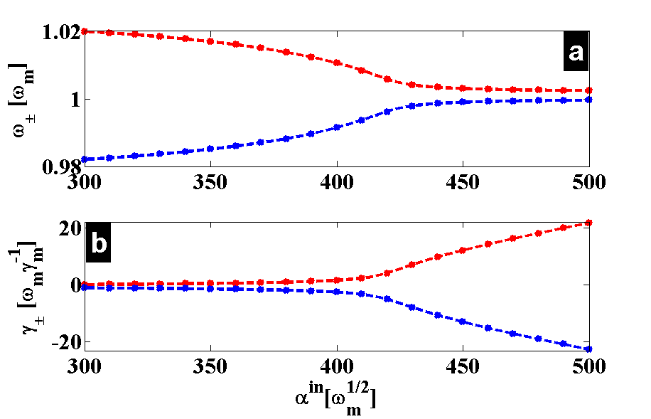
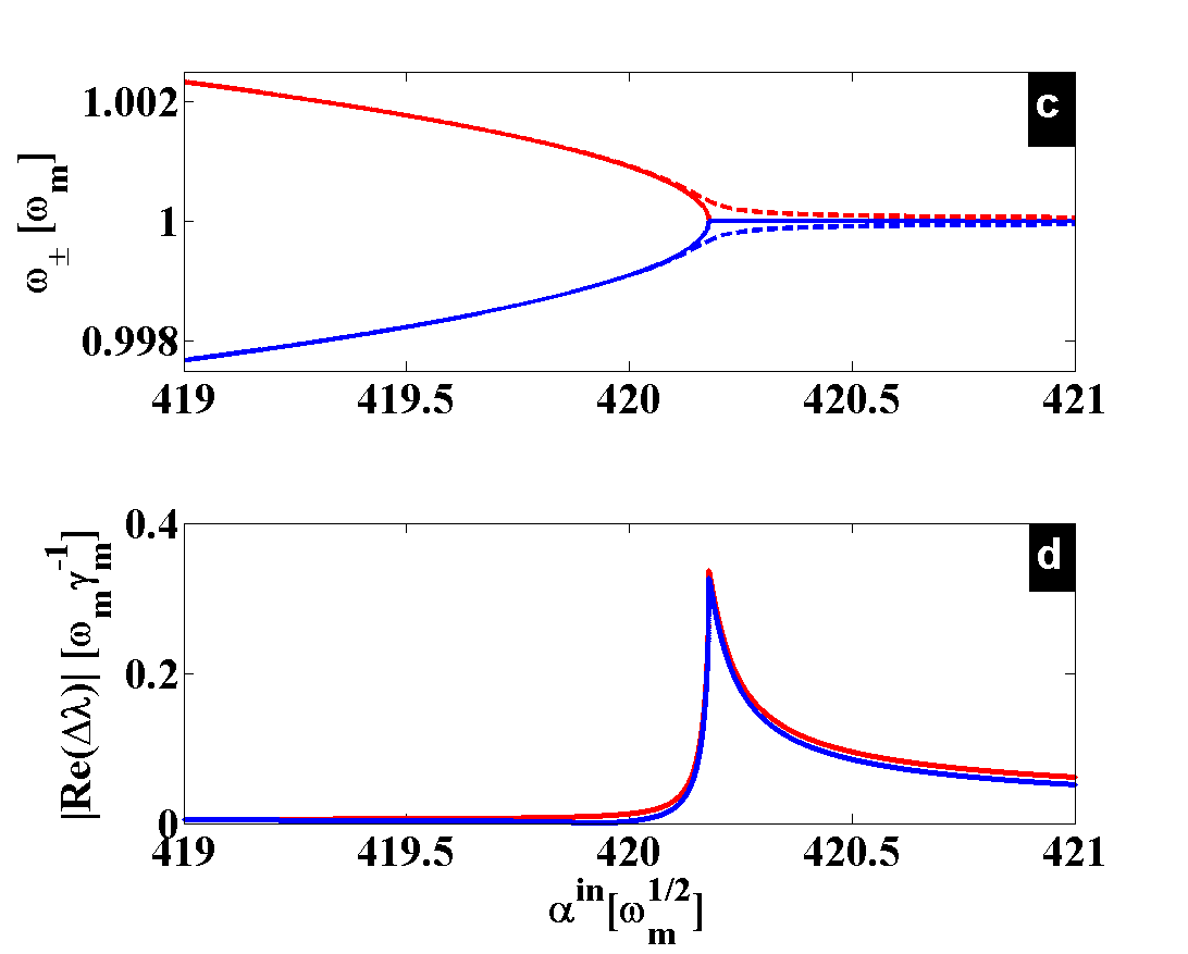
Figure 6: (a)-(b) Real and imaginary parts of the eigenvalues versus the driving field for a perturbation $\delta\omega=2\times 10^{-3}\omega_{m}$. The dashed lines are the numerical results, while the dotted lines represent the analytical approximation given in Eq. (11) and Eq. (18). This validates the approximations made in our calculations. (c)-(d) Eigenfrequencies and the corresponding sensitivities for a weak perturbation $\delta\omega=10^{-5}\omega_{m}$. One remarks that both frequencies experience the same sensitivity as predicted in our calculations.

Appendix B Frequency control through quadratic coupling

By accounting the quadratic coupling in the model, the Hamiltonian becomes,

$$H=H_{OM,ck}+H_{int}+H_{drive},$$ (24)

where $\rm{ck}$ stands for cross-Kerr, and

$$\left\{\begin{array}[c]{c}H_{OM,ck}=\sum_{j=1,2}\omega_{j}b_{j}^{{\dagger}}b_{j}-\Delta_{j}a_{j}^{{\dagger}}a_{j}\\ -ga_{j}^{{\dagger}}a_{j}(b_{j}^{{\dagger}}+b_{j})-g_{ck}a^{{\dagger}}ab^{{\dagger}}b\\ H_{int}=-J(b_{1}b_{2}^{{\dagger}}+b_{1}^{{\dagger}}b_{2})\\ H_{drive}=E(a^{{\dagger}}+a).\end{array}\right.$$ (25)

This leads to the following classical set of nonlinear equations,

$$\left\{\begin{array}[]{c}\dot{\alpha}_{1}=[i(\Delta_{1}+g(\beta_{1}^{\ast}+\beta_{1}))-\frac{\kappa}{2}]\alpha_{1}-i\sqrt{\kappa}\alpha^{\rm{in}},\\ \dot{\alpha}_{2}=[i(\Delta_{2}+g(\beta_{2}^{\ast}+\beta_{2})+g_{ck}\beta_{2}^{\ast}\beta_{2})-\frac{\kappa}{2}]\alpha_{2}-i\sqrt{\kappa}\alpha^{\rm{in}},\\ \dot{\beta}_{1}=-(i\omega_{1}+\frac{\gamma_{m}}{2})\beta_{1}+iJ\beta_{2}+ig\alpha_{1}^{\ast}\alpha_{1},\\ \dot{\beta}_{2}=-(i\tilde{\omega_{2}}+\frac{\gamma_{m}}{2})\beta_{2}+iJ\beta_{1}+ig\alpha_{2}^{\ast}\alpha_{2},\end{array}\right.$$ (26)

where $\tilde{\omega_{2}}=\omega_{2}-g_{ck}\alpha_{2}^{\ast}\alpha_{2}$ is the optically tunable mechanical frequency mentioned in the main text.

For an overview of the cross-Kerr effect, we have extended Fig. 5(a) of the main text to a large scale parameters space and for different frequency mismatch as shown in Fig. 7. One remarks that the cross-Kerr term required both to reach minimal splitting and to get closer to the EP increases as the mismatch frequency increases. This comes from the tuned frequency $\tilde{\omega_{2}}=\omega_{2}-g_{ck}\alpha_{2}^{\ast}\alpha_{2}$, which reveals the usefulness of cross-Kerr coupling not only in frequency control but also in sensitivity enhancement.

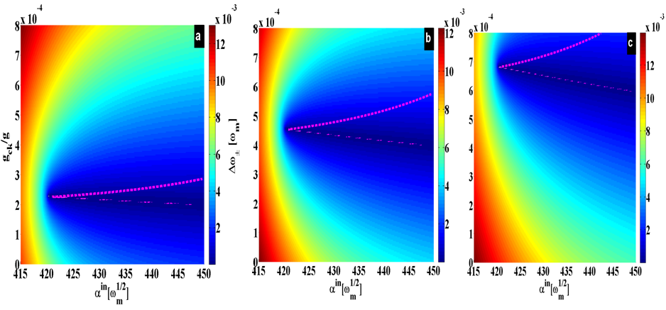
Figure 7: Diagrams showing the control strategy in ($\alpha^{in},g_{ck}$) space, at the frequency mismatches $\nu=1\times 10^{-3}\omega_{m}$, $\nu=2\times 10^{-3}\omega_{m}$ and $\nu=3\times 10^{-3}\omega_{m}$, for (a), (b), and (c) respectively. It is revealed that large mismatch frequency requires large cross-Kerr term to reach minimal splitting.

References

- (1) M. Li, H. X. Tang, and M. L. Roukes, Ultra-sensitive NEMS-based cantilevers for sensing, scanned probe and very high-frequency applications, Nature Nanotech. 2, 114 (2007).
- (2) K. L. Ekinci, X. M. H. Huang, and M. L. Roukes, Ultrasensitive nanoelectromechanical mass detection, Appl. Phys. Lett. 84, 4469 (2004).
- (3) N. V. Lavrik and P. G. Datskos, Femtogram mass detection using photothermally actuated nanomechanical resonators, Appl. Phys. Lett. 82, 2697 (2003).
- (4) B. Ilic, H. G. Craighead, S. Krylov, W. Senaratne, C. Ober, and P. Neuzil, Attogram detection using nanoelectromechanical oscillators, J. Appl. Phys. 95, 3694 (2004).
- (5) Y. T. Yang et al., Zeptogram-scale nanomechanical mass sensing, Nano Lett. 6, 583 (2006).
- (6) J. Chaste et al., A nanomechanical mass sensor with yoctogram resolution, Nature Nanotech. 7, 301 (2012).
- (7) J.-J. Li, and K.-D. Zhu, All-optical mass sensing with coupled mechanical resonator systems, Physics Reports 525, 223 (2013).
- (8) J.-J. Li, and K.-D. Zhu, Nonlinear optical mass sensor with an optomechanical microresonator, Appl. Phys. Lett. 101, 141905 (2012).
- (9) F. Liu et al., Sub-pg mass sensing and measurement with an optomechanical oscillator, Opt. Express 21, 19555 (2013).
- (10) H. Xiong, L.-G. Si, and Y. Wu, Precision measurement of electrical charges in an optomechanical system beyond linearized dynamics, Appl. Phys. Lett. 110, 171102 (2017).
- (11) C. Jiang et al., Ultrasensitive nanomechanical mass sensor using hybrid opto-electromechanical systems, Opt. Express 21, 13773 (2014).
- (12) Y. He, Sensitivity of optical mass sensor enhanced by optomechanical coupling, Appl. Phys. Lett. 106, 121905 (2015).
- (13) J. Hakansson al., Strong forces in optomechanically actuated resonant mass sensor, Opt. Express 25, 30939 (2017).
- (14) I. M. Haghighi et al., Sensitivity-Bandwidth Limit in a Multimode Optoelectromechanical Transducer, Phys. Rev. Applied 9, 034031 (2018).
- (15) T. S. Biswas et al., Time-Resolved Mass Sensing of a Molecular Adsorbate Nonuniformly Distributed Along a Nanomechnical String Phys. Rev. Applied 3, 064002 (2015).
- (16) J. Wiersig, Enhancing the sensitivity of frequency and energy splitting detection by using exceptional points: Application to microcavity sensors for single-particle detection, Phys. Rev. Lett. 112, 203901 (2014).
- (17) W. Chen et al., Exceptional points enhance sensing in an optical microcavity, Nature 548, 192 (2017); Parity-time-symmetric whispering-gallery mode nanoparticle sensor, Photonics Research 6, A23 (2018).
- (18) H. Hodaei et al., Enhanced sensitivity at higher-order exceptional points, Nature 548, 187 (2017).
- (19) Z.-P. Liu et al., Metrology with PT-Symmetric Cavities: Enhanced Sensitivity near the -Phase Transition, Phys. Rev. Lett. 117, 110802 (2016).
- (20) P. Djorwe, Y. Pennec, and B. Djafari-Rouhani, Frequency locking and controllable chaos through exceptional points in optomechanics, Phys. Rev. E 98, 032201 (2018).
- (21) T. K. Paraïso et al., Position-Squared Coupling in a Tunable Photonic Crystal Optomechanical Cavity, Phys. Rev. X 5, 041024 (2015).
- (22) J. D. Cohen et al., Phonon counting and intensity interferometry of a nanomechanical resonator, Nature 520, 522 (2015).
- (23) S. Hong et al., Hanbury Brown and Twiss interferometry of single phonons from an optomechanical resonator, Science 358, 203 (2017).
- (24) H. Xu et al., Topological energy transfer in an optomechanical system with exceptional points, Nature 537, 80 (2016).
- (25) M. Pernpeintner et al., Frequency control and coherent excitation transfer in a nanostring-resonator network, Phys. Rev. Applied 10, 034007 (2018).
- (26) H. Fu et al., Coherent optomechanical switch for motion transduction based on dynamically localized mechanical modes, Phys. Rev. Applied 9, 054024 (2018).
- (27) N. R. Bernier et al., Level attraction in microwave optomechanical circuit, Phys. Rev. A 98, 023841 (2018).