Honeycomb rare-earth magnets with anisotropic exchange interactions

Abstract

We study the rare-earth magnets on a honeycomb lattice, and are particularly interested in the experimental consequences of the highly anisotropic spin interaction due to the spin-orbit entanglement. We perform a high-temperature series expansion using a generic nearest-neighbor Hamiltonian with anisotropic interactions, and obtain the heat capacity, the parallel and perpendicular spin susceptibilities, and the magnetic torque coefficients. We further examine the electron spin resonance linewidth as an important signature of the anisotropic spin interactions. Due to the small interaction energy scale of the rare-earth moments, it is experimentally feasible to realize the strong-field regime. Therefore, we perform the spin-wave analysis and study the possibility of topological magnons when a strong field is applied to the system. The application and relevance to the rare-earth Kitaev materials are discussed.

I Introduction

Spin liquid candidates are often being searched among geometrically frustrated systems, such as triangular Anderson , kagomé Sachdev or pyrochlore Anderson1956 lattices. This is quite reasonable as the geometrical frustration could lead to a large number of degenerate or nearly-degenerate classical ground states for commonly studied Heisenberg models and thus enhance quantum fluctuations when the quantum effects are included. However, the destabilization of simple magnetically ordered states and driving a disordered one can happen even on unfrustrated lattices, by exploiting the power of anisotropic interactions Krempa ; the Kitaev honeycomb model Kitaev is a representative example of the latter. Besides being an academic interest, anisotropic spin interactions are also inevitable in realistic magnetic materials, especially those with heavy atoms. A large number of spin liquid candidates are known experimentally to possess a significant spin-orbit coupling, leading to rather anisotropic spin interactions PhysRevX.1.021002 ; Pan ; Gingras ; YbMgGa1 ; YbMgGa2 ; RuCl3 . Beyond the current interest in the spin liquid physics, understanding the relationship between the magnetic properties and the anisotropic spin interactions is a frontier topic in the field of quantum magnetism.

The most commonly studied anisotropic magnets on unfrustrated lattices are the $4d/5d$ magnets RuCl3 ; Iridates1 that include the honeycomb iridates and RuCl₃. Due to the possible proximity to Kitaev physics, these materials were referred as Kitaev materials. Due to the spatial extension of the $4d/5d$ electron wavefunctions, the exchange interactions between the local moments are usually beyond the nearest neighbors. Moreover, the iridates often suffer from a strong neutron absorption such that the data-rich neutron scattering measurement can be difficult. In comparison, the rare-earth family has the advantages of much stronger spin-orbit couplings and much more localized $4f$ orbitals PhysRevB.95.085132 ; Jang ; RauYb , and the exchange interactions often restrict to first neighbors. This makes the understanding of the modeling Hamiltonian more accessible. In addition, the rare-earth magnets do not have the neutron absorption issue that prevails in iridates. Furthermore, their smaller energy scales allow for the possibility to quantitatively understand their Hamiltonian through the external magnetic fields. However, rare-earth materials have only been well-investigated on frustrated lattices Pyrochlore1 ; YbMgGa1 .

In this paper, we will study the rare-earth magnets on the unfrustrated honeycomb lattice, and pursue an understanding of the experimental consequence of the spin-orbital entanglement on the honeycomb structure. We start by exploring the thermodynamic properties of a generic model with the nearest neighbor interactions. It is well-known that the anisotropic exchange couplings could appear in the temperature dependence of the thermodynamic quantities such as the specific heat, spin susceptibility PhysRevB.96.144414 and magnetotropic coefficients Torque ; PhysRevLett.122.197202 . Especially for the spin susceptibility and magnetic torque, magnetic fields along different directions induce magnetization of different magnitudes, leading to the anisotropic spin susceptibility PhysRevB.82.064412 ; PhysRevB.91.094422 ; PhysRevB.91.144420 ; PhysRevB.91.180401 ; freund2016single ; PhysRevB.98.100403 and the angular dependence of the magnetic torque PhysRevLett.118.187203 ; PhysRevB.98.205110 ; modic2018resonant ; PhysRevB.99.081101 , and providing a natural detection of the intrinsic spin anisotropy in the system. To go beyond the thermodynamic properties, we further consider the electron spin resonance (ESR) measurement Oshikawa ; PhysRevB.96.241107 of the system. The ESR measurement turns out to be a very sensitive probe of the magnetic anisotropy and is especially useful for the study of the strong spin-orbit-coupled quantum materials, and we compute the ESR linewidth to reveal the intrinsic spin anisotropy of the spin interactions.

Due to the small energy scale of the interaction between the rare-earth local moment, it is ready to apply a small magnetic field in the laboratory to change the magnetic state into a fully polarized one. For such a simple product state, the magnetic excitation can be readily worked out from the linear spin wave theory. We further consider the spin wave spectrum and explore the possibility of topological magnons Shindou1 ; Shindou2 ; Matsumoto ; Matsumoto1 ; Owerre1 ; Owerre2 ; LChen ; McClarty . We find the magnon spectrum supports non-trivial topological band structure. This feature can be manifested in thermal Hall transport measurements.

The remaining parts of the paper are organized as follows. In Sec. II, we introduce the nearest-neighbor spin Hamiltonian, followed by the high-temperature analysis of heat capacity, spin susceptibilities and magnetic torque coefficient in Sec III. Then we consider the ESR and calculate the influence of anisotropy on the ESR linewidth in Sec. IV. Next the linear spin wave theory of the system is exploited under strong external fields in Sec. V and the aspect of topological magnons is discussed. Finally in Sec. VI we comment on a possible material YbCl₃ and its potential realization of the Kitaev honeycomb model.

II Model

We begin with the following microscopic spin model, that is the most general nearest neighbor Hamiltonian on a honeycomb lattice with the (usual) Kramers doublet effective spin-1/2 local moments RauYb ; YbMgGa2 ; PhysRevB.94.035107 ; PhysRevX.1.021002 ,

$$H = \sum_{\langle ij\rangle}J_{zz}S_{i}^{z}S_{j}^{z}+J_{\pm}(S_{i}^{+}S_{j}^{-}+S_{i}^{-}S_{j}^{+})$$ (1)

$$+ J_{\pm\pm}(\gamma_{ij}S_{i}^{+}S_{j}^{+}+\gamma_{ij}^{*}S_{i}^{-}S_{j}^{-})$$

$$+ J_{\pm z}[(\gamma_{ij}^{*}S_{i}^{+}S_{j}^{z}+\gamma_{ij}S_{i}^{-}S_{j}^{z})+\langle i\leftrightarrow j\rangle],$$

with $\gamma_{ij}$ taking $e^{2i\pi/3}$, $e^{-2i\pi/3}$, and $1$ on the bonds along $\mathbf{a}_{1}$, $\mathbf{a}_{2}$, $\mathbf{a}_{3}$ directions respectively, as shown in Fig. 1. The spin components are defined in the global coordinate system in Fig. 1. This is possible because the system is planar and has an unique rotational axis. This differs from the rare-earth pyrochlore materials where the spins are often defined in the local coordinate system for each sublattice. This model applies to the rare-earth local moment such as the Yb³⁺ ion. For non-Kramers doublet like Pr³⁺ or Tb³⁺ ion, the $J_{\pm z}$ term is not allowed by symmetry, and the model becomes further simplified. In fact, a non-Kramers doublet based rare-earth honeycomb magnet arises from the triangular lattice magnet TbInO₃ after 1/3 of the Tb³⁺ ions becomes inactive magnetically Clark2019 . For the rare-earth local moments, the $4f$ electrons are much localized, and most often, one only needs to consider the nearest-neighbor interactions, and occasionally, one would like to include the further neighbor dipole-dipole interactions. In contrast, for the $4d/5d$ systems, one may need to worry about further neighbor exchange interactions because of the large spatial extension of the electron wavefunctions.

Figure 1: The honeycomb lattice with three different types of bonds and our choice of the global coordinate system.

An alternative and often used parametrization of the Hamiltonian is that of the $J$-$K$-$\Gamma$-$\Gamma^{\prime}$ model Rau :

$$H = \sum_{\langle ij\rangle\in\alpha\beta(\gamma)}\left[J\mathbf{S}_{i}\cdot\mathbf{S}_{j}+KS_{i}^{\gamma}S_{j}^{\gamma}+\Gamma(S_{i}^{\alpha}S_{j}^{\beta}+S_{i}^{\beta}S_{j}^{\alpha})\right]$$ (2)

$$+ \Gamma^{\prime}\sum_{\langle ij\rangle\in\alpha\beta(\gamma)}\left(S_{i}^{\alpha}S_{j}^{\gamma}+S_{i}^{\gamma}S_{j}^{\alpha}+S_{i}^{\beta}S_{j}^{\gamma}+S_{i}^{\gamma}S_{j}^{\beta}\right),$$

where $\alpha,\beta,\gamma$ take values in $\{x^{\prime},y^{\prime},z^{\prime}\}$. In the latter coordinate system, our unit vectors of Fig. 1 can be expressed by ${\hat{x}=(-1,-1,2)/\sqrt{6}}$, ${\hat{y}=(1,-1,0)/\sqrt{2}}$ and ${\hat{z}=(1,1,1)/\sqrt{3}}$. The spin components in the above equation are

$$\begin{split}&S^{x^{\prime}}=-\frac{\sqrt{6}}{6}S_{x}+\frac{\sqrt{2}}{2}S_{y}+\frac{\sqrt{3}}{3}S_{z},\\ &S^{y^{\prime}}=-\frac{\sqrt{6}}{6}S_{x}-\frac{\sqrt{2}}{2}S_{y}+\frac{\sqrt{3}}{3}S_{z},\\ &S^{z^{\prime}}=\frac{\sqrt{6}}{3}S_{x}+\frac{\sqrt{3}}{3}S_{z}.\\ \end{split}$$ (3)

Furthermore, we have used the notation that $\alpha\beta(\gamma)$ specifies a bond parallel (or anti-parallel) to the vector $\hat{{\alpha}}-\hat{{\beta}}$, or simply a bond of type $\gamma$. The coupling constants in Eq. (1) and (2) are related by the following equation

$$\begin{split}&J=\frac{4}{3}J_{\pm}-\frac{2\sqrt{2}}{3}J_{\pm z}-\frac{2}{3}J_{\pm\pm}+\frac{1}{3}J_{zz},\\ &K=2\sqrt{2}J_{\pm z}+2J_{\pm\pm},\\ &\Gamma=-\frac{2}{3}J_{\pm}-\frac{2\sqrt{2}}{3}J_{\pm z}+\frac{4}{3}J_{\pm\pm}+\frac{1}{3}J_{zz},\\ &\Gamma^{\prime}=-\frac{2}{3}J_{\pm}+\frac{\sqrt{2}}{3}J_{\pm z}-\frac{2}{3}J_{\pm\pm}+\frac{1}{3}J_{zz}.\end{split}$$ (4)

The Hamiltonian in Eq. (1) can also be used to describe the general exchange interaction between the higher spin local moments for the honeycomb magnets after some modification. The differences are explained in details in the Appendix A.

III Thermodynamics

The highly anisotropic nature of the exchange interaction first impacts the thermodynamic properties of the system. Here we explicitly calculate the specific heat and the magnetic susceptibilities of the system from the generic exchange Hamiltonian. Using the high-temperature series expansion Fisher ; HTEBook , we find the heat capacity to be

$$C=\frac{3J_{0}^{2}}{2k_{B}T^{2}}-\frac{27J_{0}^{4}}{8k_{B}^{3}T^{4}},$$ (5)

where we have

$$J_{0}^{2}\equiv\frac{1}{16}J_{zz}^{2}+\frac{1}{2}(J_{\pm}^{2}+J_{\pm\pm}^{2}+J_{\pm z}^{2}).$$ (6)

Due to the spin-orbit entanglement, the coupling of the local moment to the external magnetic field is also anisotropic. The Landé factors are different for the in-plane and out-plane magnetic fields, and the Zeeman coupling is given as

$$H_{Z}=-\mu_{0}\mu_{B}\sum_{i}\left[g_{\perp}(h_{x}S_{i}^{x}+h_{y}S_{i}^{y})+g_{\parallel}h_{\parallel}S_{i}^{z}\right].$$ (7)

Again using high-temperature series expansion, we compute the parallel and perpendicular spin susceptibilities up to $\mathcal{O}(T^{-3})$

$$\begin{split}\chi_{\parallel}=\frac{\mu_{0}\mu_{B}^{2}g_{\parallel}^{2}}{4k_{B}T}&\left(1-\frac{3J_{zz}}{4k_{B}T}-\frac{J_{\pm}^{2}}{2k_{B}^{2}T^{2}}-\frac{J_{\pm\pm}^{2}}{2k_{B}^{2}T^{2}}\right.\\ &\left.-\frac{J_{\pm z}^{2}}{k_{B}^{2}T^{2}}+\frac{3J_{zz}^{2}}{8k_{B}^{2}T^{2}}\right),\\ \chi_{\perp}=\frac{\mu_{0}\mu_{B}^{2}g_{\perp}^{2}}{4k_{B}T}&\left(1-\frac{3J_{\pm}}{2k_{B}T}+\frac{5J_{\pm}^{2}}{4k_{B}^{2}T^{2}}-\frac{J_{\pm\pm}^{2}}{k_{B}^{2}T^{2}}\right.\\ &\left.-\frac{3J_{\pm z}^{2}}{4k_{B}^{2}T^{2}}-\frac{J_{zz}^{2}}{16k_{B}^{2}T^{2}}\right).\end{split}$$ (8)

In the SU(2)-symmetric point, ${J_{zz}=2J_{\pm}},$ ${J_{\pm\pm}=J_{\pm z}=0}$, the two expressions coincide. For the rare-earth local moments with non-Kramers doublets, $g_{\perp}=0$ so $\chi_{\perp}=0$. In Fig. 2, we plot the magnetic susceptibilities and show the deviation from the simple Curie-Weiss law due to the high order anisotropic terms.

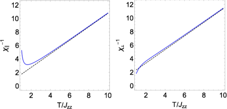
Figure 2: Susceptibilities versus temperature. The parameters are chosen to be $J_{zz}=1$, $J_{\pm}=0.9$, $J_{\pm\pm}=0.2,$ $J_{\pm z}=0.1$. The susceptibilities in the plot, $\chi_{\parallel}$ and $\chi_{\perp}$, are in units of ${\mu_{0}\mu_{B}^{2}g_{\parallel}^{2}}/{4k_{B}}$ and ${\mu_{0}\mu_{B}^{2}g_{\perp}^{2}}/{4k_{B}}$, respectively.

In addition to the simple thermodynamics such as $C_{v}$ and $\chi$, the magnetic torque measurement is proved to be quite useful in revealing the magnetic anisotropy. Intrinsically, there is because the induced magnetization is generically not parallel to the magnetic field. Thus, when the sample has an anisotropic magnetization, the system would experience a torque ${\tau=M\times H=-\partial F/\partial\theta}$ in an external magnetic field. The magnetotropic coefficient ${k=\partial^{2}F/\partial\theta^{2}}$, defined as the second derivative of the free energy to the angle $\theta$ between the sample and the applied magnetic field, can be introduced to quantify such anisotropy. It can be directly measured using the resonant torsion magnetometry Torque . Under the high temperature expansion, we find the magnetotropic coefficient $k$ is given as

$$\begin{split}k=&\frac{\mu_{0}^{2}\mu_{B}^{2}h^{2}}{k_{B}T}\cos 2\theta\big{\{}\frac{1}{4}(g_{\perp}^{2}-g_{\parallel}^{2})+\frac{3}{16k_{B}T}(g_{\parallel}^{2}J_{zz}-2g_{\perp}^{2}J_{\pm})\\ &+\frac{1}{192k_{B}^{2}T^{2}}\big{[}-3g_{\perp}^{2}(-20J_{\pm}^{2}+16J_{\pm\pm}^{2}+12J_{\pm z}^{2}+J_{zz}^{2})\\ &+6g_{\parallel}^{2}(4J_{\pm}^{2}+4J_{\pm\pm}^{2}+8J_{\pm z}^{2}-3J_{zz}^{2})\\ &-2\mu_{0}^{2}\mu_{B}^{2}h^{2}(g_{\perp}^{4}-g_{\parallel}^{4})\big{]}\big{\}}-\frac{\mu_{0}^{4}\mu_{B}^{4}h^{4}}{96k_{B}^{3}T^{3}}\cos 4\theta(g_{\perp}^{2}-g_{\parallel}^{2})^{2},\end{split}$$ (9)

where we have defined $h^{2}=h_{x}^{2}+h_{y}^{2}+h_{z}^{2}.$ The coefficient $k$ vanishes in the g-isotropic $g_{\perp}=g_{\parallel}$ and Heisenberg limit: ${J_{zz}=2J_{\pm}}$, ${J_{\pm\pm}=J_{\pm z}=0}$. More details of the calculation can be found in Appendix B.

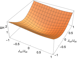
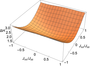
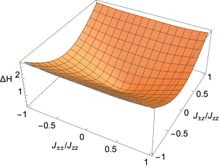
Figure 3: (Color online.) The dependence of $\Delta H$ on $J_{\pm\pm}$ and $J_{\pm z}$. Left: $J_{\pm}/J_{zz}=1$, middle: $J_{\pm}/J_{zz}=-0.5$, right: $J_{\pm}/J_{zz}=0.2$. The linewidth $\Delta H$ in the three plots are in the units $\mu_{B}g(\theta)/\sqrt{2\pi}$.

IV Electron spin resonance

In the thermodynamic properties, the leading contributions come from the $J_{zz}$ and $J_{\pm}$ terms, while the $J_{\pm\pm}$ and $J_{\pm z}$ terms are subleading. Arising from spin-orbital entanglement and completely breaking the U(1) rotational symmetry, these terms play important roles in the potential quantum spin liquid behavior. To resolve them, we now turn to the electron spin resonance.

Electron spin resonance measures the absorption of electromagnetic radiation by a sample subjected to an external static magnetic field. For a SU(2) invariant system, the absorption is completely sharp, i.e. described by a delta function located exactly at the Zeeman energy Oshikawa . Therefore, the broadening of the resonance spectrum has to arise from the magnetic anisotropy. To understand the contribution of the anisotropy of the nearest-neighbor spin interaction to the ESR linewidth, we decompose the Hamiltonian Eq. (1) into the isotropic Heisenberg part and the anisotropic exchange part

$$H=J\sum_{\langle i,j\rangle}\mathbf{S}_{i}\cdot\mathbf{S}_{j}+H^{\prime},$$ (10)

where the Heisenberg coupling $J=(J_{zz}+4J_{\pm})/3$, and the anisotropic part

$$H^{\prime}=\sum_{\langle i,j\rangle}S_{i}^{\mu}\,\Gamma_{ij,\mu\nu}\,S_{j}^{\nu}.$$ (11)

Here $\Gamma_{ij}$ a traceless and symmetric exchange coupling matrix, satisfying

$$\begin{split}&\Gamma_{ij,xx}=2J_{\pm}/3+(\gamma_{ij}+\gamma_{ij}^{*})J_{\pm\pm}-J_{zz}/3,\\ &\Gamma_{ij,yy}=2J_{\pm}/3-(\gamma_{ij}+\gamma_{ij}^{*})J_{\pm\pm}-J_{zz}/3,\\ &\Gamma_{ij,xy}=i(\gamma_{ij}-\gamma_{ij}^{*})J_{\pm\pm},\\ &\Gamma_{ij,yz}=i(\gamma_{ij}^{*}-\gamma_{ij})J_{\pm z},\\ &\Gamma_{ij,zx}=(\gamma_{ij}+\gamma_{ij}^{*})J_{\pm z}.\end{split}$$ (12)

Under the Zeeman term of Eq. (7), the ESR linewidth for a Lorentzian-shaped spectrum is Linewidth ; Castner ; Soos

$$\Delta H(\theta)=\frac{\sqrt{2\pi}}{\mu_{B}g(\theta)}\left(\frac{M_{2}^{3}}{M_{4}}\right)^{1/2},$$ (13)

where $\theta$ is again the angle between the external field and the sample, and

$$g(\theta) = \sqrt{g_{\parallel}^{2}\sin^{2}\theta+g_{\perp}^{2}\cos^{2}\theta},$$ (14)

$$M_{2} = \frac{\langle[H^{\prime},M^{+}][M^{-},H^{\prime}]\rangle}{\langle M^{+}M^{-}\rangle},$$ (15)

$$M_{4} = \frac{\langle[H,[H^{\prime},M^{+}]][H,[H^{\prime},M^{-}]]\rangle}{\langle M^{+}M^{-}\rangle}.$$ (16)

$M_{2}$ and $M_{4}$ are the second and the fourth moments, respectively, and $M^{\pm}\equiv\sum_{i}S_{i}^{\pm}$. The expectation “$\langle\cdots\rangle$”in the above equations is taken with respect to high temperatures. Specifically, we find that

$$\begin{split}M_{2}=&\frac{3}{4}(J_{zz}^{2}+4J_{\pm}^{2}+4J_{\pm\pm}^{2}+10J_{\pm z}^{2}-4J_{\pm}J_{zz}),\\ M_{4}=&\frac{3}{4}J_{zz}^{4}-\frac{9}{2}J_{zz}^{3}J_{\pm}+\frac{57}{8}J_{zz}^{2}J_{\pm z}^{2}+15J_{zz}^{2}J_{\pm}^{2}\\ &+6J_{zz}^{2}J_{\pm\pm}^{2}-\frac{3}{4}J_{zz}J_{\pm\pm}J_{\pm z}^{2}-\frac{93}{4}J_{zz}J_{\pm}J_{\pm z}^{2}\\ &-24J_{zz}J_{\pm}J_{\pm\pm}^{2}-30J_{zz}J_{\pm}^{3}+\frac{123}{2}J_{\pm z}^{4}\\ &+\frac{153}{2}J_{\pm\pm}^{2}J_{\pm z}^{2}+\frac{39}{2}J_{\pm}J_{\pm\pm}J_{\pm z}^{2}+33J_{\pm}^{2}J_{\pm z}^{2}\\ &+15J_{\pm\pm}^{4}+30J_{\pm}^{2}J_{\pm\pm}^{2}+24J_{\pm}^{4}.\end{split}$$ (17)

Our result for ESR linewidths can be compared to the future ESR experiments on the rare-earth based honeycomb magnets in order to extract the anisotropic exchanges. In Fig. 3, we further depict the three-dimensional plots that explicitly demonstrate the dependence of the ESR linewidth on the anisotropic couplings $J_{z\pm}$ and ${J_{\pm\pm}}$ for three different choices of $J_{\pm}$.

V Polarized phases

V.1 Strong field normal to the honeycomb plane

To further explore the effect of the anisotropic exchange interaction, we study the spin wave excitation with respect to the polarized states under the strong magnetic fields. This is clearly feasible in the current laboratory setting for the rare-earth magnets as the energy scales for them are usually rather small. For the $4d/5d$ magnets, there can be difficulty to achieve as the energy scale over there is much higher. Our results here are relevant to the inelastic neutron scattering and thermal Hall transport measurements.

We first consider the case of a strong magnetic field in the direction normal to the honeycomb plane such that the system is in the fully polarized paramagnetic phase and all the spins are aligned along the $z$ direction. In this case, the magnon bands carry nontrivial Chern numbers for generic range of parameters, as found in reference McClarty in the $J-K-\Gamma-\Gamma^{\prime}$ presentation. We expand about this fully polarized state using the conventional Holstein-Primakoff transformations of the spin variables Holstein , which are ${S_{i}^{z}=S-a_{i}^{\dagger}a_{i},S_{i}^{+}=a_{i},S_{i}^{-}=a_{i}^{\dagger}}$ for sublattice A, and substitute $a\rightarrow b$ for sublattice B. $a$ and $b$’s are bosonic operators, $[a_{i},a_{j}^{\dagger}]=[b_{i},b_{j}^{\dagger}]=\delta_{ij}$. Keeping only the bilinear terms of bosonic operators and taking the Fourier transformation, we arrive at

$$H=\frac{3N}{4}J_{zz}-2N\mu_{0}\mu_{B}g_{\parallel}h_{z}+\frac{1}{2}\Upsilon_{\mathbf{k}}^{\dagger}\mathcal{H}_{\mathbf{k}}\Upsilon_{\mathbf{k}},\$$ (18)

with ${\Upsilon\equiv(a_{\mathbf{k}},b_{\mathbf{k}},a_{-\mathbf{k}}^{\dagger},b_{-\mathbf{k}}^{\dagger})^{T}}$. Here we have denoted ${k_{1}=-\frac{1}{2}k_{x}+\frac{\sqrt{3}}{2}k_{y}},{k_{2}=-\frac{1}{2}k_{x}-\frac{\sqrt{3}}{2}k_{y}}$, and ${k_{3}=k_{x}}$ that correspond to the $y$-, $z$- and $x$-bonds, respectively. We further define ${f(\mathbf{k})=\sum_{i}e^{ik_{i}}}$, ${g_{1}(\mathbf{k})=\sum_{i}e^{-ik_{i}}\gamma_{i}}$, ${g_{2}(\mathbf{k})=\sum_{i}e^{ik_{i}}\gamma_{i}}$ and $u\equiv(g_{\parallel}\mu_{0}\mu_{B}h_{\parallel}-3J_{zz}/2)$, we then have for $\mathcal{H}_{\mathbf{k}}$ a block form

$$\mathcal{H}_{\mathbf{k}}=\left[\begin{matrix}A(\mathbf{k})&B(\mathbf{k})\\ B^{\dagger}(\mathbf{k})&A^{T}(-\mathbf{k})\end{matrix}\right],$$ (19)

where we have

$$A(\mathbf{k}) = \left[\begin{matrix}u&J_{\pm}f^{*}\\ J_{\pm}f&u\end{matrix}\right],$$ (20)

$$B^{\dagger}(\mathbf{k}) = \left[\begin{matrix}0&J_{\pm\pm}g_{1}\\ J_{\pm\pm}g_{2}&0\end{matrix}\right].$$ (21)

All the $J_{\pm z}$ terms are not present.

The spin wave dispersion relation for $\mathcal{H}_{\mathbf{k}}$ follows as

$$\begin{split}\epsilon(\mathbf{k})^{2}=&u^{2}+|f|^{2}J_{\pm}^{2}-\frac{|g_{1}|^{2}+|g_{2}|^{2}}{\sqrt{2}}J_{\pm\pm}^{2}\\ &\pm[4|f|^{2}u^{2}J_{\pm}^{2}+\frac{|g_{1}|^{2}-|g_{2}|^{2}}{4}J_{\pm\pm}^{4}\\ &+(f^{*}g_{1}^{*}-fg_{2}^{*})(f^{*}g_{2}-fg_{1})J_{\pm}^{2}J_{\pm\pm}^{2}]^{1/2},\end{split}$$ (22)

where only the positive square root of $\epsilon(\mathbf{k})^{2}$ is taken.

Several simple limits of this expression can be checked: (1) in the Heisenberg limit $J_{zz}=2J_{\pm}\equiv 2J$, then $\epsilon(\mathbf{k})=(\frac{g_{\parallel}\mu_{0}\mu_{B}}{2S}h_{\parallel}-3J\pm|f|J)^{1/2}$; (2) when only $J_{zz}$ is finite, it reduces to the Ising case $\epsilon(\mathbf{k})=\frac{g_{\parallel}\mu_{0}\mu_{B}}{2S}h_{\parallel}-\frac{3}{2}J_{zz}$; if only $J_{\pm}$ is present, we have a graphene-like dispersion $\epsilon(\mathbf{k})=\frac{g_{\parallel}\mu_{0}\mu_{B}}{2S}h_{\parallel}\pm|f|J_{\pm}$.

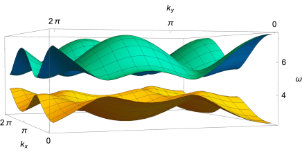
Figure 4: (Color online.) The two spin wave bands $\omega_{\pm}$ when a strong field in the $z$-direction is applied. The parameters are chosen as ${J_{zz}=1;J_{\pm}=0.9;J_{\pm\pm}=1;J_{\pm z}=0.3;u=5}$.

At high fields, the results can be simplified by the Schrieffer-Wolff transformation,

$$\tilde{\mathcal{H}}_{\mathbf{k}} = e^{W}\mathcal{H}_{\mathbf{k}}e^{-W}$$ (23)

$$= \mathcal{H}_{\mathbf{k}}+[W,\mathcal{H}_{\mathbf{k}}]+\frac{1}{2}\big{[}W,[W,\mathcal{H}_{\mathbf{k}}]\big{]}+\cdots,$$

with the commutator understood as

$$[X,Y]\equiv X\eta Y-Y\eta X,$$ (24)

and $\eta$ is a diagonal matrix with entries $(1,1,-1,-1)$. Following the treatment of Ref. McClarty , we choose the transformation to be

$$W=\frac{1}{2u}\left(\begin{matrix}0&B(\mathbf{k})\\ -B^{\dagger}(\mathbf{k})&0\end{matrix}\right),$$ (25)

so that up to $O(h_{\parallel}^{-2})$, we have the $\tilde{\mathcal{H}}_{\mathbf{k}}$ to become $A(\mathbf{k})\rightarrow\tilde{A}(\mathbf{k})$, $B(\mathbf{k})\rightarrow\tilde{B}(\mathbf{k})$,

$$\begin{split}&\tilde{A}(\mathbf{k})=\left(\begin{matrix}u-\frac{J_{\pm\pm}^{2}}{2u}|g_{2}|^{2}&f^{*}J_{\pm}\\ fJ_{\pm}&u-\frac{J_{\pm\pm}^{2}}{2u}|g_{1}|^{2}\end{matrix}\right),\\ &\tilde{B}(\mathbf{k})=-\frac{J_{\pm}J_{\pm\pm}}{2u}\left(\begin{matrix}f^{*}g_{1}^{*}+g_{2}^{*}f&0\\ 0&f^{*}g_{1}^{*}+g_{2}^{*}f\end{matrix}\right).\end{split}$$ (26)

At high fields, we can thus ignore $\tilde{B}(\mathbf{k})$ and focus on the $\tilde{A}(\mathbf{k})$ term. Writing $\tilde{A}(\mathbf{k})=d_{0}(\mathbf{k})\mathbbm{1}+\frac{1}{2}\mathbf{d}(\mathbf{k})\cdot{\boldsymbol{\sigma}},$ with the three components being

$$d_{1}(\mathbf{k}) = 2J_{\pm}~{}Re(f),$$ (27)

$$d_{2}(\mathbf{k}) = 2J_{\pm}~{}Im(f),$$ (28)

$$d_{3}(\mathbf{k}) = \frac{J_{\pm\pm}^{2}}{2u}(|g_{1}|^{2}-|g_{2}|^{2}),$$ (29)

$$d_{0}(\mathbf{k}) = u-\frac{J_{\pm\pm}^{2}}{4u}(|g_{1}|^{2}+|g_{2}|^{2}).$$ (30)

At each momentum $\mathbf{k}$ we have the eigenvalues

$$\omega_{\pm}(\mathbf{k})=d_{0}(\mathbf{k})\pm\frac{1}{2}|\mathbf{d}(\mathbf{k})|.$$ (31)

The above spin wave bands Eq. (31) do not touch unless $J_{\pm}=J_{\pm\pm}=0$, as we have depicted in Fig. 4. We further compute the Berry curvature as follows

$$F_{\pm}^{xy}(\mathbf{k})=\pm\frac{i}{2}\left[\frac{\mathbf{d}(\mathbf{k})}{|\mathbf{d}(\mathbf{k})|^{3}}\cdot\left(\frac{\partial\mathbf{d}(\mathbf{k})}{\partial k_{y}}\times\frac{\partial\mathbf{d}(\mathbf{k})}{\partial k_{x}}\right)\right].$$ (32)

This is negative semi-definite in the Brillouin zone. The Chern numbers follow as

$$C_{\pm}=\frac{1}{2\pi i}\int_{BZ}dk_{x}dk_{y}F_{\pm}^{xy}=\mp 1.$$ (33)

This implies the presence of chiral magnon edge states and thermal Hall effect, resulting from the presence of magnon number non-conserving terms $B(\mathbf{k})$ in the Hamiltonian Matsumoto ; McClarty . The edge state for the open boundary condition is depicted in Fig. 5.

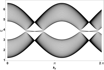
Figure 5: Edge state in a cylindrical geometry. The $y$-direction is periodic, while $x$-direction contains 50 sites. The parameters are $J_{zz}=1,$ $J_{\pm}=0.9,$ $J_{\pm\pm}=0.6,$ $u=4.$

V.2 Strong field in the honeycomb plane

We now turn to a strong in-plane field, in the $x$-direction. This is relevant for the rare-earth local moments with the usual Kramers doublet, and does not apply to the non-Kramers doublet. The Holstein-Primakoff transformation for sublattice A is modified as $S_{i}^{x}=\frac{1}{2}-a_{i}^{\dagger}a_{i},S_{i}^{y}=\frac{1}{2}(a_{i}+a_{i}^{\dagger}),S_{i}^{z}=\frac{1}{2i}(a_{i}-a_{i}^{\dagger})$, and that for sublattice B is obtained by substituting $a$ by $b$. These are again bosonic operators satisfying $[a_{i},a_{j}^{\dagger}]=[b_{i},b_{j}^{\dagger}]=\delta_{ij}$. Keeping only the bilinear terms of bosonic operators and taking the Fourier transformation, we obtain

$$H = \frac{3N}{2}J_{\pm}-2N\mu_{0}\mu_{B}g_{\perp}h_{x}+\frac{1}{2}\Upsilon_{\mathbf{k}}^{\dagger}\mathcal{H}_{\mathbf{k}}\Upsilon_{\mathbf{k}},$$ (34)

$$\Upsilon \equiv (a_{\mathbf{k}},b_{\mathbf{k}},a_{-\mathbf{k}}^{\dagger},b_{-\mathbf{k}}^{\dagger})^{T}.$$ (35)

Define $g_{3}(\mathbf{k})=e^{ik_{1}}+e^{ik_{2}}-2e^{ik_{3}}$, $g_{4}(\mathbf{k})=e^{ik_{1}}-e^{ik_{2}}$ and recall $f(\mathbf{k})=\sum_{i}e^{ik_{i}}$. The $\mathcal{H}_{k}$ is of the familiar form

$$\mathcal{H}_{\mathbf{k}}=\left[\begin{matrix}A(\mathbf{k})&B(\mathbf{k})\\ B^{\dagger}(\mathbf{k})&A^{T}(-\mathbf{k})\end{matrix}\right],$$

but now with the $A,B$ matrices given by

$$A(\mathbf{k})_{11}=A(\mathbf{k})_{22}=v=\mu_{0}\mu_{B}g_{\perp}h_{x}-3J_{\pm},$$ (36)

$$A(\mathbf{k})_{21}=A(\mathbf{-k})_{12}=(\frac{1}{4}J_{zz}+\frac{1}{2}J_{\pm})f+\frac{g_{3}}{4}J_{\pm\pm},$$ (37)

$$B(\mathbf{k})_{11}=B(\mathbf{k})_{22}=0,$$ (38)

$$B(\mathbf{k})_{21}=B(\mathbf{-k})_{12}=(-\frac{1}{4}J_{zz}+\frac{1}{2}J_{\pm})f$$

$$\quad\quad\quad\quad\quad\quad\quad+\frac{1}{4}J_{\pm\pm}g_{3}+\frac{i\sqrt{3}}{2}J_{\pm z}g_{4}.$$ (39)

Appealing again to the Schrieffer-Wolff transformation with

$$W=\frac{1}{2v}\left(\begin{matrix}0&B(\mathbf{k})\\ -B^{\dagger}(\mathbf{k})&0\end{matrix}\right),$$ (40)

then up to $O(h_{\perp}^{-2})$, we have the effective $\tilde{\mathcal{H}}_{k}$ to be $A(\mathbf{k})\rightarrow\tilde{A}(\mathbf{k})$, $B(\mathbf{k})\rightarrow\tilde{B}(\mathbf{k})$.

$$\tilde{A}(\mathbf{k})=\left(\begin{matrix}v-\frac{1}{2v}|B(\mathbf{k})_{12}|^{2}&A(\mathbf{k})_{12}\\ A(\mathbf{k})_{21}&v-\frac{1}{2v}|B(\mathbf{k})_{21}|^{2}\end{matrix}\right),$$ (41)

$$\tilde{B}(\mathbf{k})=-\frac{\mathbbm{1}}{2v}\big{[}A(\mathbf{k})_{21}B(\mathbf{k})_{12}+A(\mathbf{k})_{12}B(\mathbf{k})_{21}\big{]}.$$ (42)

At high fields $h_{\perp}$, we can ignore $\tilde{B}(\mathbf{k})$ and focus on the $\tilde{A}(\mathbf{k})$ term. Rewrite $\tilde{A}(\mathbf{k})=d_{0}(k)\mathbbm{1}+\frac{1}{2}\mathbf{d}(\mathbf{k})\cdot\mathbf{\sigma}$, with each component being

$$d_{1}=(\frac{1}{4}J_{zz}+\frac{1}{2}J_{\pm})Re(f)+\frac{1}{4}J_{\pm\pm}Re(g_{3}),$$ (43)

$$d_{2}=(\frac{1}{4}J_{zz}+\frac{1}{2}J_{\pm})Im(f)+\frac{1}{4}J_{\pm\pm}Im(g_{3}),$$ (44)

$$d_{3}=-\frac{1}{2v}\big{[}i\frac{\sqrt{3}}{2}g_{4}^{*}J_{\pm z}[(\frac{1}{4}J_{zz}+\frac{1}{2}J_{\pm})f+\frac{1}{4}J_{\pm\pm}g_{3}]$$

$$\quad\quad\quad\quad\quad\quad\quad\quad\quad+c.c\big{]},$$ (45)

$$d_{0}=v-\frac{1}{2v}[(\frac{1}{4}J_{zz}+\frac{1}{2}J_{\pm})^{2}|f|^{2}+\frac{3}{4}J_{\pm z}^{2}|g_{4}|^{2}].$$ (46)

We then arrive at the dispersions $\omega_{\pm}(\mathbf{k})=d_{0}(\mathbf{k})\pm\frac{1}{2}|\mathbf{d}(\mathbf{k})|$. The spectrum is plotted in Fig. 6. We find both bands have zero Chern numbers, and we have checked for many other parameter choices and also obtained trivial zero Chern number. Thus, the in-plane field magnon band structure is quite distinct from the topological magnon band structure for the normal-plane field case.

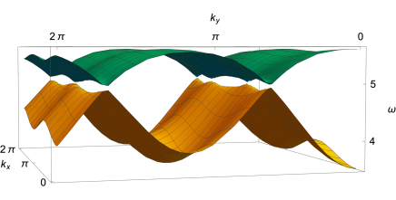
Figure 6: (Color online.) The two spin wave bands $\omega_{\pm}$ when a strong in-plane field is present. The parameters are chosen $J_{zz}=1$; $J_{\pm}=0.9$; $J_{\pm\pm}=1$; $J_{\pm z}=0.3$; $v=5$.

VI Discussion

We have studied the experimental consequences of the spin-orbital entanglement and the anisotropic spin exchange interactions in the honeycomb rare-earth magnets. These results can be directly compared with the experiments, thereby providing a useful guidance for the future study on candidate systems. One future direction would be to involve higher-lying crystal field states based on the information of specific materials.

One potential rare-earth candidate for the anisotropic honeycomb lattice model is YbCl₃ Chemistry , which has a similar crystal structure to that of RuCl₃. The Yb³⁺ ions have nearly filled $4f$-orbitals, which, combined with the large crystal fields lead to Kramers doublet ground state manifold. This is modeled as an effective spin-1/2 local moment. Furthermore, its edge-shared octahedral structure gives simple exchange physics that is relatively well-understood according to a microscopic calculation in Ref. RauYb, . There is very limited information about this material in the literature apart from a very recent work Ni .

In this paper, we have focused the analysis on the honeycomb lattice rare-earth magnets and its anisotropic interaction. It is noticed that, the generic model for the rare-earth honeycomb magnets contains a Kitaev interaction as one independent exchange interaction out of four. It is thus reasonable for us to consider the possibility of Kitaev materials among the honeycomb rare-earth magnets. In fact most rare-earth magnets have not been discussed along the line of Kitaev interactions, except the first few works PhysRevB.95.085132 ; Jang ; RauYb . In the previous work PhysRevB.95.085132 , we have illustrated this observation with the FCC rare-earth magnets. Since many non-honeycomb lattice iridates are claimed as Kitaev materials, it is thus reasonable to consider the rare-earth magnets with other crystal structures to be potential Kitaev materials beyond the previously proposed ones and the honeycomb one here RauMichel ; PhysRevLett.119.057203 . The reason that these rare-earth magnets contain a Kitaev interaction is due to two facts. The first fact is the spin-obital-entangled effective spin-1/2 local moment. The second fact is the three-fold rotation symmetry at the lattice site. This symmetry permutes the effective spin components and generates a Kitaev interaction. These two ingredients can be used as the recipe to search for other rare-earth Kitaev materials beyond the honeycomb one.

To summarize, we have focused on rare-earth honeycomb materials with nearest-neighbor interactions and computed the high-temperature thermodynamic properties, ESR linewidth, and spin-wave behaviors as the experimental consequences of the anisotropic spin interaction.

VII Acknowledgments

We thank Leon Balents, Ni Ni, and Jiaqiang Yan for conversations. Gang Chen thanks Prof Peng Xue for her hospitality during the visit to Beijing Computational Science Research Center where this work is completed. This work is supported by the Ministry of Science and Technology of China with the Grant No.2016YFA0301001,2016YFA0300500,2018YFE0103200, by from the Research Grants Council of Hong Kong with General Research Fund Grant No.17303819, by the Heising-Simons Foundation, and the National Science Foundation under Grant No. NSF PHY-1748958.

Appendix A Generic spin models and candidate states for higher spins

This spin model in Eq. (1) is designed for effective spin-1/2 local moments. It can be well extended to the high-spin local moments. For the honeycomb lattice with spin-1 local moments, the pairwise spin interaction is given as

$$\begin{split}H=&\sum_{\langle ij\rangle}J_{zz}S_{i}^{z}S_{j}^{z}+J_{\pm}(S_{i}^{+}S_{j}^{-}+S_{i}^{-}S_{j}^{+})\\ &+J_{\pm\pm}(\gamma_{ij}S_{i}^{+}S_{j}^{+}+\gamma_{ij}^{*}S_{i}^{-}S_{j}^{-})\\ &+J_{\pm z}[(\gamma_{ij}^{*}S_{i}^{+}S_{j}^{z}+\gamma_{ij}S_{i}^{-}S_{j}^{z})+\langle i\leftrightarrow j\rangle]\\ &+\sum_{i}D(S_{i}^{z})^{2}.\end{split}$$ (47)

Because of the larger Hilbert space, a single-ion anisotropy is allowed and new states such as the quantum paramagnet can be favored here. Thus, the phase transitions between quantum paramagnet and other ordered phases can be interesting. Further neighbor exchange interaction, if included, could bring more frustration channel than the spin-orbit entanglement induced frustration. It is known that, simple $J_{1}$-$J_{2}$ (first neighbor and second neighbor Heisenberg) model on honeycomb lattice could induce spiral spin liquids in two dimensions where the spiral degeneracy has a line degeneracy in the momentum space rather than the surface degeneracy. The presence of the anisotropic interaction in Eq. (47) would overcome the quantum/classical order by disorder effect and lift the degeneracy. In addition to the spin-1 local moments, the model in Eq. (47) also applies to the spin-3/2 systems. Since the honeycomb lattice contains three nearest neighbor bonds, one may consider the possibility of the ALKT states on the honeycomb lattice where the nearest neighbor bonds are covered with spin singles of the spin-1/2 states and three onsite spin-1/2 spins are combined back to a spin-3/2 local moments.

Here, we have only listed the pairwise spin interactions. Due to the spin-orbital entanglement and the spin-lattice coupling, the effective interaction for the spin-1 and spin-3/2 magnets can contain significant multipolar interactions. A simple example would be the biquadratic exchange $-({\boldsymbol{S}}_{i}\cdot{\boldsymbol{S}}_{j})^{2}$ that is induced effectively by the spin-lattice coupling. The presence of these multipolar interactions can significantly enhance quantum fluctuation by allowing the system to tunnel more effectively within the local spin Hilbert space and thus create more quantum states such as multipolar ordered phases and quantum spin liquids PhysRevB.84.094420 ; PhysRevB.82.174440 .

The relevant physical systems for the spin-1 and spin-3/2 moments would contain the $4d^{2},5d^{2},4d^{4},5d^{4}$ and $4d^{1},5d^{1},4d^{3},5d^{3}$ magnetic ions, respectively. The relevant ions can arise from Ru, Mo and even V atoms, where spin-orbit coupling in the partially filled $t_{2g}$ shell is active PhysRevB.84.094420 ; PhysRevB.82.174440 .

Appendix B Details of high temperature expansion

The high temperature expansion requires to take into account the commutation relations between different spin operators on a same site. To this end, we define a vertex function $\nu_{i}(n_{x},n_{y},n_{z})$ at each site $i$ following Ref. Fisher, , where $n_{x},n_{y}$ and $n_{z}$ have to be even integers for the function to be nonzero. Its explicit form can be calculated by introducing the generating function

$$\psi(\xi,\eta,\zeta)=\text{Tr}~{}\left[\exp(\xi S^{x}+\eta S^{y}+\zeta S^{z})\right].$$ (48)

Expanding the exponential and using the definition of $\nu$, we have

$$\psi(\xi,\eta,\zeta)=2\sum_{n_{x}=0}^{\infty}\sum_{n_{y}=0}^{\infty}\sum_{n_{z}=0}^{\infty}\frac{\nu(n_{x},n_{y},n_{z})}{2^{n_{x}+n_{y}+n_{z}}}\frac{\xi^{n_{x}}\eta^{n_{y}}\zeta^{n_{z}}}{n_{x}!n_{y}!n_{z}!}.$$ (49)

On the other hand, by diagonalizing the matrix of the exponential, we have

$$\psi(\xi,\eta,\zeta)=2\cosh\left(\sqrt{\xi^{2}+\eta^{2}+\zeta^{2}}/2\right).$$ (50)

Expanding this and comparing with the previous equation,

$$\nu(n_{x},n_{y},n_{z})=\frac{[(n_{x}+n_{y}+n_{z})/2]!}{(n_{x}/2)!(n_{y}/2)!(n_{z}/2)!}\frac{n_{x}!n_{y}!n_{z}!}{(n_{x}+n_{y}+n_{z})!}.$$ (51)

We note this function is symmetric under the permutation of $n_{x},n_{y},n_{z}$. The heat capacity is related to the zero-field partition function in the following way

$$C=\frac{1}{N}\frac{\partial E}{\partial T}=\frac{\beta^{2}}{N}\left[\frac{1}{Z_{0}}\frac{\partial^{2}Z_{0}}{\partial\beta^{2}}-\frac{1}{Z_{0}^{2}}\left(\frac{\partial Z_{0}}{\partial\beta}\right)^{2}\right],$$ (52)

where we have divided by the number of sites $N$ to get the intensive quantity. $Z_{0}$ is given by

$$Z_{0}=2^{N}\left[1+\frac{1}{4}\beta^{2}\sum_{\langle ij\rangle}(\frac{1}{8}J_{zz}^{2}+J_{\pm}^{2}+J_{\pm\pm}^{2}+J_{\pm z}^{2})\right]+O(\beta^{3}),$$ (53)

where the $2^{N}$ factor results from the summation over all possible configurations.

Susceptibility in direction $a$ can be reduced to the following expectation values of two spin operators,

$$\chi_{a}=\frac{1}{\beta N}\frac{\partial^{2}}{\partial h_{a}^{2}}\ln Z\big{|}_{h_{a}=0}=\frac{\mu_{0}\mu_{B}^{2}g_{a}^{2}}{NZ_{0}}\beta\langle\sum_{m,n}S_{m}^{a}S_{n}^{a}\rangle_{0}.$$ (54)

Using the vertex function $\nu(n_{x},n_{y},n_{z})$ defined above, we obtain for the parallel case,

$$\begin{split}&\langle\sum_{m,n}S_{m}^{z}S_{n}^{z}\rangle_{0}=\sum_{\{\mathbf{S}_{i}\}}\sum_{m,n}S_{m}^{z}S_{n}^{z}e^{-\beta H}\\ =&\sum_{\{\mathbf{S}_{i}\}}\left[\sum_{m,n}S_{m}^{z}S_{n}^{z}-\beta\sum_{\langle ij\rangle}\sum_{m,n}H_{ij}S_{m}^{z}S_{n}^{z}+\frac{1}{2}\beta^{2}\sum_{\langle ij\rangle}\sum_{\langle kl\rangle}\sum_{m,n}H_{ij}H_{kl}S_{m}^{z}S_{n}^{z}+\text{permutations}+O(\beta^{3})\right]\\ =&\sum_{\{\mathbf{S}_{i}\}}\left\{\frac{N}{4}-\frac{3N}{16}\beta J_{zz}+\frac{3N}{128}\beta^{2}J_{zz}^{2}+(\frac{3N^{2}}{32}-\frac{3N}{16})\beta^{2}(\frac{1}{8}J_{zz}^{2}+J_{\pm}^{2}+J_{\pm\pm}^{2}+J_{\pm z}^{2})\right.\\ &+\frac{\beta^{2}}{32}(J_{\pm}^{2}+J_{\pm\pm}^{2})\sum_{\langle ij\rangle}\left[\nu_{i}(2,0,2)\nu_{j}(2,0,0)+\nu_{i}(2,0,2)\nu_{j}(0,2,0)+\nu_{i}(0,2,2)\nu_{j}(2,0,0)+\nu_{i}(0,2,2)\nu_{j}(0,2,0)\right]\\ &+\frac{\beta^{2}}{32}J_{\pm z}^{2}\sum_{\langle ij\rangle}\left[\nu_{i}(2,0,2)\nu_{j}(0,0,2)+\nu_{i}(0,2,2)\nu_{j}(0,0,2)+\nu_{i}(0,0,4)\nu_{j}(2,0,0)+\nu_{i}(0,0,4)\nu_{j}(0,2,0)\right]\\ &\left.+\frac{1}{16}\beta^{2}\sum_{\langle ij\rangle}(J_{zz}^{2}-2J_{\pm z}^{2})+O(\beta^{3})\right\}\\ =&2^{N}\cdot\frac{N}{4}\left[1-\frac{3}{4}\beta J_{zz}+\beta^{2}(\frac{3}{8}J_{zz}^{2}-\frac{1}{2}J_{\pm}^{2}-\frac{1}{2}J_{\pm\pm}^{2}-J_{\pm z}^{2})+\frac{3N}{8}\beta^{2}(\frac{1}{8}J_{zz}^{2}+J_{\pm}^{2}+J_{\pm\pm}^{2}+J_{\pm z}^{2})+O(\beta^{3})\right].\end{split}$$ (55)

Here, the summation for $\{\mathbf{S}_{i}\}$ is over the possible configurations of spins on all sites. The notation $H_{ij}$ means the terms in the Hamiltonian for the bond labeled by sites $i,j$; namely, $H=\sum_{\langle ij\rangle}H_{ij}$.“Permutations” on the second line are those with respect to the relative orderings of $H_{ij},$ $H_{kl},$ $S_{m}^{z}$ and $S_{n}^{z}$.

Similarly, for the perpendicular susceptibility, we have

$$\begin{split}&\langle\sum_{m,n}S_{m}^{x}S_{n}^{x}\rangle_{0}=\sum_{\{\mathbf{S}_{i}\}}\sum_{m,n}S_{m}^{x}S_{n}^{x}e^{-\beta H}\\ =&\sum_{\{\mathbf{S}_{i}\}}\left[\sum_{m,n}S_{m}^{x}S_{n}^{x}-\beta\sum_{\langle ij\rangle}\sum_{m,n}H_{ij}S_{m}^{x}S_{n}^{x}+\frac{1}{2}\beta^{2}\sum_{\langle ij\rangle}\sum_{\langle kl\rangle}\sum_{m,n}H_{ij}H_{kl}S_{m}^{x}S_{n}^{x}+\text{permutations}+O(\beta^{3})\right]\\ =&\sum_{\{\mathbf{S}_{i}\}}\left\{\frac{N}{4}-\frac{3N}{8}\beta J_{\pm}+\frac{N-2}{16}\beta^{2}\sum_{\langle ij\rangle}(\frac{1}{8}J_{zz}^{2}+J_{\pm}^{2}+J_{\pm\pm}^{2}+J_{\pm z}^{2})+\frac{1}{64}\beta^{2}J_{zz}^{2}\sum_{\langle ij\rangle}\nu_{i}(2,0,2)\nu_{j}(0,0,2)\right.\\ &+\frac{1}{32}\beta^{2}(J_{\pm}^{2}+J_{\pm\pm}^{2})\sum_{\langle ij\rangle}[\nu_{i}(4,0,0)\nu_{j}(2,0,0)+\nu_{i}(4,0,0)\nu_{j}(0,2,0)+\nu_{i}(2,2,0)\nu_{j}(2,0,0)+\nu_{i}(2,2,0)\nu_{j}(0,2,0)]\\ &+\frac{1}{32}\beta^{2}J_{\pm z}^{2}\sum_{\langle ij\rangle}[\nu_{i}(4,0,0)\nu_{j}(0,0,2)+\nu_{i}(2,2,0)\nu_{j}(0,0,2)+\nu_{i}(2,0,2)\nu_{j}(2,0,0)+\nu_{i}(2,0,2)\nu_{j}(0,2,0)]\\ \end{split}$$

$$\begin{split}&\left.+\beta^{2}\sum_{\langle ij\rangle}\sum_{\langle jk\rangle}\left[\frac{1}{8}J_{\pm}^{2}+\frac{1}{16}J_{\pm\pm}^{2}(\gamma_{ij}\gamma_{jk}^{*}+\gamma_{ij}^{*}\gamma_{jk})+\frac{1}{32}J_{\pm z}^{2}(\gamma_{ij}\gamma_{jk}+\gamma_{ij}\gamma_{jk}^{*}+c.c)\right]+O(\beta^{3})\right\}\\ =&2^{N}\cdot\frac{N}{4}\left[1-\frac{3}{2}\beta J_{\pm}+\frac{3N}{8}\beta^{2}(\frac{1}{8}J_{zz}^{2}+J_{\pm}^{2}+J_{\pm\pm}^{2}+J_{\pm z}^{2})-\frac{1}{16}\beta^{2}J_{zz}^{2}+\frac{5}{4}\beta^{2}J_{\pm}^{2}-\beta^{2}J_{\pm\pm}^{2}-\frac{3}{4}\beta^{2}J_{\pm z}^{2}+O(\beta^{3})\right].\end{split}$$ (56)

The magnetotropic coefficient $k$ can be computed using its relationship with the partition function with non-zero external field,

$$k=\frac{1}{N}\frac{\partial^{2}F}{\partial\theta^{2}}=\frac{1}{\beta N}\left[\frac{1}{Z^{2}}\left(\frac{\partial Z}{\partial\theta}\right)^{2}-\frac{1}{Z}\frac{\partial^{2}Z}{\partial\theta^{2}}\right].$$ (57)

The first term always give higher order terms compared with the second term, while the latter reads,

$$\begin{split}\frac{\partial^{2}Z}{\partial\theta^{2}}=&-\beta\mu_{0}\mu_{B}\sum_{i}\langle g_{\perp}\cos\theta(\cos\varphi S_{i}^{x}+\sin\varphi S_{i}^{y})+g_{\parallel}\sin\theta S_{i}^{z}\rangle+\beta^{2}\mu_{0}^{2}\mu_{B}^{2}\sum_{i,j}\langle g_{\perp}^{2}\sin^{2}\theta\cos^{2}\varphi S_{i}^{x}S_{j}^{x}+g_{\perp}^{2}\sin^{2}\theta\sin^{2}\varphi S_{i}^{y}S_{j}^{y}\\ &+g_{\parallel}^{2}\cos^{2}\theta S_{i}^{z}S_{j}^{z}-g_{\perp}g_{\parallel}\sin\theta\cos\theta\cos\varphi(S_{i}^{z}S_{j}^{x}+S_{i}^{x}S_{j}^{z})-g_{\perp}g_{\parallel}\sin\theta\cos\theta\sin\varphi(S_{i}^{z}S_{j}^{y}+S_{i}^{y}S_{j}^{z})\\ &+g_{\perp}^{2}\sin^{2}\theta\sin\varphi\cos\varphi(S_{i}^{x}S_{j}^{y}+S_{i}^{y}S_{j}^{x})\rangle+O(\beta^{3})\\ =&\mu_{0}^{2}\mu_{B}^{2}\beta^{2}\cos 2\theta(g_{\parallel}^{2}-g_{\perp}^{2})+\frac{3\mu_{0}^{2}\mu_{B}^{2}}{4}\beta^{3}\cos 2\theta(2g_{\perp}^{2}J_{\pm}-g_{\parallel}^{2}J_{zz})-\frac{\mu_{0}^{4}\mu_{B}^{4}}{48}\beta^{4}\cos 4\theta(g_{\perp}^{2}-g_{\parallel}^{2})^{2}(3N-2)\\ &-\frac{\mu_{0}^{2}\mu_{B}^{2}}{192}\beta^{4}\cos 2\theta\left\{3N(g_{\perp}^{2}-g_{\parallel}^{2})\left[4\mu_{0}^{2}\mu_{B}^{2}(g_{\perp}^{2}+g_{\parallel}^{2})+3(J_{zz}^{2}+8J_{\pm}^{2}+8J_{\pm\pm}^{2}+8J_{\pm z}^{2})\right]\right.\\ &-\left.4\left[2\mu_{0}^{2}\mu_{B}^{2}(g_{\perp}^{4}-g_{\parallel}^{4})-6g_{\parallel}^{2}(-3J_{zz}^{2}+4J_{\pm}^{2}+4J_{\pm\pm}^{2}+8J_{\pm z}^{2})+3g_{\perp}^{2}(J_{zz}^{2}-20J_{\pm}^{2}+16J_{\pm\pm}^{2}+12J_{\pm z}^{2})\right]\right\}.\end{split}$$ (58)

The expression above reduces to, in the limit $g_{\perp}=g_{\parallel}$,

$$\frac{\partial^{2}Z}{\partial\theta^{2}}\big{|}_{g_{\perp}=g_{\parallel}}=2^{N}\cdot\frac{N}{4}\beta^{3}\mu_{0}^{2}\mu_{B}^{2}\cos 2\theta\left[-12J_{zz}+24J_{\pm}+\beta(7J_{zz}^{2}-28J_{\pm}^{2}+8J_{\pm\pm}^{2}-4J_{\pm z}^{2})\right].$$ (59)

References

- (1) P. W. Anderson. Resonating valence bonds: a new kind of insulator? Mat. Res. Bull., 8:153–160, 1973.
- (2) S. Sachdev. Kagome´- and triangular-lattice Heisenberg antiferromagnets: Ordering from quantum fluctuations and quantum-disordered ground states with unconfined bosonic spinons. Phys. Rev. B, 45:12377, 1992.
- (3) P. W. Anderson. Ordering and Antiferromagnetism in Ferrites. Phys. Rev., 102:1008, 1956.
- (4) W. Witczak-Krempa, G. Chen, Y. B. Kim, and L. Balents. Correlated quantum phenomena in the strong spin-orbit regime. Annu. Rev. Condens. Matter Phys., 5:57–82, 2014.
- (5) Alexei Kitaev. Anyons in an exactly solved model and beyond. Annals of Physics, 321(1):2 – 111, 2006.
- (6) Kate A. Ross, Lucile Savary, Bruce D. Gaulin, and Leon Balents. Quantum Excitations in Quantum Spin Ice. Phys. Rev. X, 1:021002, Oct 2011.
- (7) L. Pan, S. K. Kim, A. Ghosh, C. M. Morris, K. A. Ross, E. Kermarrec, B. D. Gaulin, S. M. Koohpayeh, O. Tchernyshyov, and N. P. Armitage. Low-energy electrodynamics of novel spin excitations in the quantum spin ice Yb2Ti2O7. Nat. Commun., 5:4970, 2014.
- (8) M. J. P. Gingras and P. A. McClarty. Quantum Spin Ice: A Search for Gapless Quantum Spin Liquids in Pyrochlore Magnets. Rep. Prog. Phys., 77:056501, 2014.
- (9) Y. Li, H. Liao, Z. Zhang, F. Jin S. Li, L. Ling, L. Zhang, Y. Zou, L. Pi, Z. Yang, J. Wang, Z. Wu, and Q. Zhang. Gapless quantum spin liquid ground state in the two-dimensional spin- triangular antiferromagnet . Sci. Rep., 5:16419, 2015.
- (10) Y. Li, G. Chen, W. Tong, L. Pi, J. Liu, Z. Yang, X. Wang, and Q. Zhang. Rare-earth triangular lattice spin liquid: A single-crystal study of . Phys. Rev. Lett., 115:167203, 2015.
- (11) A Banerjee, CA Bridges, J-Q Yan, AA Aczel, L Li, MB Stone, GE Granroth, MD Lumsden, Y Yiu, J Knolle, et al. Proximate kitaev quantum spin liquid behaviour in a honeycomb magnet. Nature materials, 15:733–740, 2016.
- (12) G. Jackeli and G. Khaliullin. Mott insulators in the strong spin-orbit coupling limit: From heisenberg to a quantum compass and kitaev models. Phys. Rev. Lett., 102:017205, Jan 2009.
- (13) Fei-Ye Li, Yao-Dong Li, Yue Yu, Arun Paramekanti, and Gang Chen. Kitaev materials beyond iridates: Order by quantum disorder and Weyl magnons in rare-earth double perovskites. Phys. Rev. B, 95:085132, Feb 2017.
- (14) S.-H. Jang, R. Sano, Y. Kato, and Y. Motome. Antiferromagnetic Kitaev Interaction in -Electron Based Honeycomb Magnets. Phys. Rev. B, 99:241106, 2019.
- (15) J .G. Rau and M. J. P. Gingras. Frustration and anisotropic exchange in ytterbium magnets with edge-shared octahedra. Phys. Rev. B, 98:054408, 2018.
- (16) J. S. Gardner, M. J. P. Gingras, and J. E. Greedan. Magnetic pyrochlore oxides. Rev. Mod. Phys., 82(53), 2010.
- (17) R. R. P. Singh and J. Oitmaa. High-temperature thermodynamics of the honeycomb-lattice kitaev-heisenberg model: A high-temperature series expansion study. Phys. Rev. B, 96:144414, Oct 2017.
- (18) K. A. Modic, Maja D. Bachmann, B. J. Ramshaw, F. Arnold, K. R. Shirer, Amelia Estry, J. B. Betts, Nirmal J. Ghimire, E. D. Bauer, M. Schmidt, M. Baenitz, E. Svanidze, R. D. McDonald, A. Shekhter, and P. J. W. Moll. Resonant torsion magnetometry in anisotropic quantum materials. Nat. Commun., 9:3975, 2018.
- (19) Kira Riedl, Ying Li, Stephen M. Winter, and Roser Valentí. Sawtooth torque in anisotropic magnets: Application to . Phys. Rev. Lett., 122:197202, May 2019.
- (20) Yogesh Singh and P. Gegenwart. Antiferromagnetic mott insulating state in single crystals of the honeycomb lattice material . Phys. Rev. B, 82:064412, Aug 2010.
- (21) Yumi Kubota, Hidekazu Tanaka, Toshio Ono, Yasuo Narumi, and Koichi Kindo. Successive magnetic phase transitions in : Xy-like frustrated magnet on the honeycomb lattice. Phys. Rev. B, 91:094422, Mar 2015.
- (22) J. A. Sears, M. Songvilay, K. W. Plumb, J. P. Clancy, Y. Qiu, Y. Zhao, D. Parshall, and Young-June Kim. Magnetic order in : A honeycomb-lattice quantum magnet with strong spin-orbit coupling. Phys. Rev. B, 91:144420, Apr 2015.
- (23) M. Majumder, M. Schmidt, H. Rosner, A. A. Tsirlin, H. Yasuoka, and M. Baenitz. Anisotropic magnetism in the honeycomb system: Susceptibility, specific heat, and zero-field nmr. Phys. Rev. B, 91:180401, May 2015.
- (24) Florian Freund, SC Williams, RD Johnson, R Coldea, Philipp Gegenwart, and Anton Jesche. Single crystal growth from separated educts and its application to lithium transition-metal oxides. Scientific reports, 6:35362, 2016.
- (25) P. Lampen-Kelley, S. Rachel, J. Reuther, J.-Q. Yan, A. Banerjee, C. A. Bridges, H. B. Cao, S. E. Nagler, and D. Mandrus. Anisotropic susceptibilities in the honeycomb kitaev system . Phys. Rev. B, 98:100403, Sep 2018.
- (26) Ian A. Leahy, Christopher A. Pocs, Peter E. Siegfried, David Graf, S.-H. Do, Kwang-Yong Choi, B. Normand, and Minhyea Lee. Anomalous thermal conductivity and magnetic torque response in the honeycomb magnet . Phys. Rev. Lett., 118:187203, May 2017.
- (27) K. A. Modic, B. J. Ramshaw, A. Shekhter, and C. M. Varma. Chiral spin order in some purported kitaev spin-liquid compounds. Phys. Rev. B, 98:205110, Nov 2018.
- (28) KA Modic, Maja D Bachmann, BJ Ramshaw, F Arnold, KR Shirer, Amelia Estry, JB Betts, Nirmal J Ghimire, ED Bauer, Marcus Schmidt, et al. Resonant torsion magnetometry in anisotropic quantum materials. Nature communications, 9(1):1–8, 2018.
- (29) Sitikantha D. Das, Sarbajaya Kundu, Zengwei Zhu, Eundeok Mun, Ross D. McDonald, Gang Li, Luis Balicas, Alix McCollam, Gang Cao, Jeffrey G. Rau, Hae-Young Kee, Vikram Tripathi, and Suchitra E. Sebastian. Magnetic anisotropy of the alkali iridate at high magnetic fields: Evidence for strong ferromagnetic kitaev correlations. Phys. Rev. B, 99:081101, Feb 2019.
- (30) M. Oshikawa and I. Affleck. Electron spin resonance in s=1/2 antiferromagnetic chains. Phys. Rev. B, 65(134410), 2002.
- (31) A. N. Ponomaryov, E. Schulze, J. Wosnitza, P. Lampen-Kelley, A. Banerjee, J.-Q. Yan, C. A. Bridges, D. G. Mandrus, S. E. Nagler, A. K. Kolezhuk, and S. A. Zvyagin. Unconventional spin dynamics in the honeycomb-lattice material : High-field electron spin resonance studies. Phys. Rev. B, 96:241107, Dec 2017.
- (32) R. Shindou, R. Matsumoto, S. Murakami, and J.-I. Ohe. Topological chiral magnonic edge mode in a magnonic crystal. Phys. Rev. B, 87:174427, 2013.
- (33) R. Shindou, R. Matsumoto, S. Murakami, and J.-I. Ohe. Chiral spin-wave edge modes in dipolar magnetic thin films. Phys. Rev. B, 87:174402, 2013.
- (34) R. Matsumoto and S. Murakami. Rotational motion of magnons and the thermal hall effect. Phys. Rev. B, 84:184406, 2011.
- (35) R. Matsumoto, R. Shindou, and S. Murakami. Thermal hall effect of magnons in magnets with dipolar interactions. Phys. Rev. B, 89:054420, 2014.
- (36) S. A. Owerre. A first theoretical realization of honeycomb topological magnon insulator. J. Phys.: Condens. Matter, 28:386001, 2016.
- (37) S. A. Owerre. Topological honeycomb magnon hall effect: A calculation of thermal hall conductivity of magnetic spin excitations. J. Appl. Phys., 120:043903, 2016.
- (38) L. Chen, J.-H. Chung, B. Gao, T. Chen, M. B. Stone, A. I. Kolesnikov, Q. Huang, and P. Dai. Topological spin excitations in honeycomb ferromagnet CrI3. Phys. Rev. X, 8:041028, 2018.
- (39) P. A. McClarty, X.-Y. Dong, M. Gohlke, J. G. Rau, F. Pollman, R. Moessner, and K. Penc. Topological magnons in kitaev magnets at high fields. Phys. Rev. B, 98:060404, 2018.
- (40) Yao-Dong Li, Xiaoqun Wang, and Gang Chen. Anisotropic spin model of strong spin-orbit-coupled triangular antiferromagnets. Phys. Rev. B, 94:035107, Jul 2016.
- (41) Lucy Clark, Gabriele Sala, Dalini D. Maharaj, Matthew B. Stone, Kevin S. Knight, Mark T. F. Telling, Xueyun Wang, Xianghan Xu, Jaewook Kim, Yanbin Li, Sang-Wook Cheong, and Bruce D. Gaulin. Two-dimensional spin liquid behaviour in the triangular-honeycomb antiferromagnet TbInO3. Nature Physics, 15:262–268, 2019.
- (42) J. G. Rau, E. K.-H. Lee, and H.-Y. Kee. Generic spin model for the honeycomb iridates beyond the kitaev limit. Phys. Rev. Lett., 112:077204, 2014.
- (43) M. E. Fisher. Perpendicular susceptibility of the ising model. J. Math. Phys., 4:124, 1963.
- (44) J. Oitmaa, C. Hamer, and W. Zheng. Series Expansion Methods for Strongly Interacting Lattice Models. Cambridge University Press, Cambridge, 2006.
- (45) A. Abragam. The Principles of Nuclear Magnetism. Oxford University Press, London, 1961.
- (46) T. G. Castner Jr. and M. S. Seehra. Antisymmetric exchange and exchange-narrowed electron-paramagnetic-resonance linewidths. Phys. Rev. B, 4:38, 1971.
- (47) Z. G. Soos, K. T. McGregor, T. T. P. Cheung, and A. J. Silverstein. Antisymmetric and anisotropic exchange in ferromagnetic copper(ii) layers. Phys. Rev. B, 16:3036, 1977.
- (48) T. Holstein and H. Primakoff. Field dependence of the intrinsic domain magnetization of a ferromagnet. Phys. Rev., 58:1098, 1940.
- (49) D. H. Templeton and G. F. Carter. The crystal structure of yttrium trichloride and similar compounds. J. Phys. Chem., 58(11):940–944, 1954.
- (50) J. Xing, H. Cao, E. Emmanouilidou, C. Hu, J. Liu, D. Graf, A. P. Ramirez, G. Chen, and N. Ni. A rare-earth Kitaev material candidate YbCl3. arXiv:1903.03615, 2018.
- (51) Jeffrey G. Rau and Michel J.P. Gingras. Frustrated Quantum Rare-Earth Pyrochlores. Annual Review of Condensed Matter Physics, 10(1):null, 2019.
- (52) J. D. Thompson, P. A. McClarty, D. Prabhakaran, I. Cabrera, T. Guidi, and R. Coldea. Quasiparticle Breakdown and Spin Hamiltonian of the Frustrated Quantum Pyrochlore in a Magnetic Field. Phys. Rev. Lett., 119:057203, Aug 2017.
- (53) Gang Chen and Leon Balents. Spin-orbit coupling in ordered double perovskites. Phys. Rev. B, 84:094420, Sep 2011.
- (54) Gang Chen, Rodrigo Pereira, and Leon Balents. Exotic phases induced by strong spin-orbit coupling in ordered double perovskites. Phys. Rev. B, 82:174440, Nov 2010.