The formation of compact dwarf ellipticals through merging star clusters

Abstract

In the last decades, extended old stellar clusters have been observed. These extended objects cover a large range in masses, from extended clusters or faint fuzzies to ultra compact dwarf galaxies. It has been demonstrated that these extended objects can be the result of the merging of star clusters in cluster complexes (small regions in which dozens to hundreds of star clusters form). This formation channel is called the “Merging Star Cluster Scenario”. This work tries to explain the formation of compact ellipticals in the same theoretical framework. Compact ellipticals are a comparatively rare class of spheroidal galaxies, possessing very small effective radii and high central surface brightnesses. With the use of numerical simulations we show that the merging star cluster scenario, adopted for higher masses, as found with those galaxies, can reproduce all major characteristics and the dynamics of these objects. This opens up a new formation channel to explain the existence of compact elliptical galaxies.

1 Introduction

In the last decades, extended old stellar clusters have been observed. They are similar to globular clusters (GCs) but with larger sizes. As there is no clear division between the two classes of objects but rather a smooth, continuous distribution of sizes, an arbitrary limit of $R_{\rm eff}=10$ pc is currently used to distinguish between the different objects (see e.g. Brüns & Kroupa, 2012). Extended objects (EOs) cover a wide range of masses. Objects at the low mass end with masses comparable to normal GCs are called extended clusters (ECs) (e.g. Huxor et al., 2005; Chandar et al., 2004) or faint fuzzies (FFs) (Brodie & Larsen, 2002; Burkert et al., 2005) and objects at the high-mass end are called ultra compact dwarf galaxies (UCDs Hilker et al., 1999; Drinkwater et al., 2000). Ultra compact dwarf galaxies are compact objects with luminosities above the brightest known GCs. Again there is no clear boundary between high-mass GCs and low-mass UCDs, so usually, a lower mass limit of $2\cdot 10^{6}$ M_⊙ is applied.

A few decades ago young massive star clusters (YMCs) were found with GC properties in gas-rich galaxies. They are abundant in star-burst and interacting galaxies, but they are also present in some apparently unperturbed disk galaxies (Larsen & Richtler, 1999). Observations have shown that YMCs are often not isolated, but are part of larger structures (e.g. Whitmore et al., 1999) which were later dubbed cluster complexes (Brüns et al., 2009, 2011). The CCs contain from a few dozens to hundreds of young massive star clusters spanning up to a few hundred parsec in diameter. The mass of a CC is the sum of the YMC in it. Observations show that most CCs have a massive concentration of star clusters in their centres and from a few to hundreds of isolated SC in their vicinity.

Fellhauer & Kroupa (2002a, b) demonstrated that objects like ECs, FFs and UCDs can be the remnants of the merging of star cluster complexes (CCs); they called it the Merging Star Cluster Scenario. The star clusters inside of CCs are bound to each other and therefore experience constant encounters, which finally leads to a merging process of most or even all SCs inside the complex. The resulting object is massive and has a larger effective radius than the single constituents. A more concise study was performed by Brüns et al. (2009, 2011).

Our work tries to explain the formation of compact ellipticals (cEs). These objects are a comparatively rare class of spheroidal galaxies, possessing very small effective radii ($R_{\rm eff}$) defined as the projected radius that encloses half of the total luminosity of one object. The central surface brightness is high, compared to dwarf ellipticals of the same size (Faber, 1973). One of the most important characteristic of cEs is the high stellar density due the high surface brightness and the small $R_{\rm eff}$. The prototype galaxy for this type of galaxy is the 32nd object in the catalog of Messier (Messier, 1784), called M32, which is a satellite of the Andromeda galaxy (M31). Until a few years ago only about a dozen of these objects were identified up to a distance of about $100$ Mpc but in the last years their number increased significantly (Chilingarian & Zolotukhin, 2015; Janz et al., 2016; Ferré-Mateu et al., 2017).

M32 has an $R_{\rm eff}$ of the bulge of $27$ arcseconds ($\sim 100$ pc), an effective surface brightness in the bulge of $18.23$ R-mag arcsec^-2 (Graham, 2002) and a velocity dispersion of $76\pm 10$ km s^-1 (van der Marel et al., 1998).

The standard formation scenario of these systems proposes a galaxy origin. CEs are the result of tidal stripping and the truncation of nucleated larger systems (Faber, 1973). The most recent simulations by Du et al. (2018) show that by including ram pressure into the simulations the high metallicity of cEs can be explained. Or they could be a natural extension of the class of elliptical galaxies to lower luminosities and smaller sizes (Wirth & Gallagher, 1984; Kormendy et al., 2009). Kormendy & Bender (2012) argue against the stripping scenario as “not all cEs are companions of massive galaxies”.

Huxor et al. (2011) report two cEs which show evidence of formation resulting from ongoing tidal stripping of more massive progenitors, i.e. the tidal tails are clearly visible. But later Huxor et al. (2013) found the first isolated cE. Its isolated position suggests that the stripping scenario may not be the only possible formation channel. Chilingarian & Zolotukhin (2015) report that isolated cEs may be ejected from their host systems.

We want to propose a completely new formation scenario for cEs. In our project we try to model cEs in a similar way like UCDs in Fellhauer & Kroupa (2002a), which are objects with characteristics very similar to cE: high surface brightness and small $R_{\rm eff}$, i.e. high stellar density, using the merging star cluster scenario extended to higher masses and sizes. We think that in the early Universe we might have produced sufficiently strong star bursts to form cluster complexes which merge into cEs. So far it is observationally unknown if cEs are dark matter dominated objects. If our scenario is true, then they (or at least some of them) would be dark matter free, very extended and massive ”star clusters”.

2 Setup

For our cE models we divide the total mass of the cluster complex of $M_{\rm cc}=10^{9}$ M_⊙ (this initial mass of the CC is kept constant in all our simulations) into $N_{0}=64$ or $128$ ’UCDs’:

$$M_{\rm sc,64} = \frac{M_{\rm cc}}{N_{0}}\ =\ \frac{10^{9}{\rm M_{\odot}}}{64}\ =\ 15,625,000\ {\rm M_{\odot}},$$ (1)

$$M_{\rm sc,128} = \frac{10^{9}{\rm M_{\odot}}}{128}\ =\ 7,812,500\ {\rm M_{\odot}}.$$ (2)

As one can see, the term UCD is justified because our star clusters inside the CC have masses larger than the adopted mass-limit for UCDs. As this and previous studies have shown, the number of objects $N_{0}$ does not alter the results and therefore we are confident to obtain qualitatively similar results if we would have divided the total mass of the CC into more and smaller constituents. The same reasoning applies for all SCs having the same mass, even though observations show a power-law mass-spectrum $\propto M^{-2}$. Applying the correct mass function would mean that for every massive SC of mass $10^{6}$ M_⊙ we would have to simulate 100 SCs of $10^{5}$ and even 10,000 SCs of $10^{4}$ M_⊙. This is beyond the capacities of the used computer systems. Smaller simulations using a shallower mass spectrum are reported in Fellhauer & Kroupa (2003) and show no differences.

The constituents (star clusters or UCDs) are modeled as Plummer spheres (Plummer, 1911) using $100,000$ particles. The size of the SCs $R_{\rm sc}$ is varied to be $4$, $10$ or $20$ pc, with masses according to Eqs. 1 and 2. These scale radii cover the observed values of YMC and most UCDs (Whitmore et al., 1999; Maraston et al., 2004). The star clusters then are distributed inside the CC according to another Plummer distribution with a scale radius of $R_{\rm cc}$ being $50$, $100$ or $200$ pc. This choice reflects sizes seen with CCs in various observations (Whitmore et al., 1999; Bastian et al., 2005). It also is the range of initial values which could produce final merger objects similar to cEs. For all Plummer distributions we choose a cut-off radius equal to five Plummer radii. An overview over this parameters is given in Tab. 1.

Table 1: Parameters varied in the simulations. The distance to the center of the galaxy of the CC ($R_{gal}$), the Plummer radius of the SCs ($R_{sc}$), the Plummer radius of the cluster complex ($R_{cc}$) and the initial number of ’UCDs’ in the CC ($N_{0}$).

$R_{\rm gal}$	[kpc]	20	60	100
$R_{\rm sc}$	[pc]	4	10	20
$R_{\rm cc}$	[pc]	50	100	200
$N_{0}$		64	128

We simulate models with and without tidal field (at different galactic distances). The tidal field is modeled as a standard galactic potential as it is often used to model the Milky Way (Mizutani et al., 2003) leading to a rotational velocity of about $220$ km s^-1 at the solar radius and an almost flat rotation curve further out. The chosen galactic distances and the resulting parameters are shown in Tab. 2.

Table 2: Parameters for the chosen orbits. First column shows the distance to the centre of the galaxy of the CC. Second column shows the circular velocity at this distance. Third column gives the time the CC and later the merger object needs to perform one orbit around the galaxy. Last column gives the number of orbits the simulation performs, given a standard simulation time of $10$ Gyr.

$R_{\rm gal}$	$v_{\rm circ}$	$T_{\rm orb}$	$N_{\rm revol.}$
$[$kpc]	[km s-1]	[Gyr]
20	230.0	0.534	18.7
60	206.6	1.778	5.6
100	219.8	2.795	3.6

There $R_{\rm gal}$ is the distance to the center of the galaxy of the distribution of SCs/UCDs, $v_{\rm circ}$ is the initial velocity of the distribution to have a circular orbit, T_orb is the orbital period and $N_{\rm revol}$ is the number of revolutions and it is given by $\frac{\rm t_{\rm int}=10{\rm Gyr}}{\rm T_{\rm orb}}$, where $t_{\rm int}$ is our simulations time which is always $10$ Gyr.

We perform the simulations using the particle-mesh code Superbox (Fellhauer et al., 2000). Superbox is a particle-multi-mesh code with high-resolution sub-grids, which stay focused on the moving objects.

To get a good resolution of the star clusters, the individual high resolution grids cover an entire star cluster, whereas the medium resolution grids of every star cluster embed the whole initial CC. The outermost grid covers the whole orbit of the CC around the galaxy.

We perform in total 162 simulations. 81 simulations with initially $N_{0}=64$ and then similar simulations with $N_{0}=128$. For each combination of $R_{\rm gal}$, $R_{\rm sc}$ and $R_{\rm cc}$ (27 possible combinations) we perform three random realisations of the positions and velocities of the SCs inside the CC to assess the possible spread of our results.

3 Results

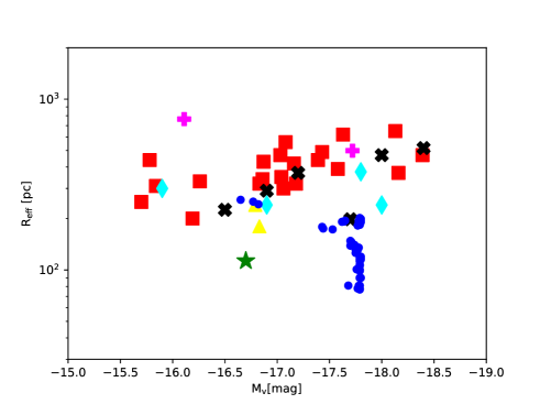
Figure 1: Absolute Magnitude vs. effective radius of observed cEs and our simulations. The green star denotes M32. The symbols are the different observational values taken from Chilingarian et al. (2007) (yellow triangles), Chilingarian et al. (2009) (red squares), Huxor et al. (2013) (magenta plus), Misgeld & Hilker (2011) (black crosses) and Norris et al. (2014) (cyan diamonds). The blue circles are our simulation results. Note that in order to determine the absolute magnitude we applied a generic M/L-ratio of unity, i.e. our objects should be less bright in reality. Furthermore, all our models have the same initial mass, therefore the final mass (or brightness) is also almost the same.

In all simulations, the merging process leads to a stable object which we are analysing after $10$ Gyr of simulation time.

Table 3: Results of the simulations of cEs. The name of the simulations (first column) is according to the size of a single SC/UCD ($R_{\rm sc}$; $4$=A, $10$=B, $20$=C), the size of the distribution or CC ($R_{\rm cc}$; $50$=a, $100$=b, $200$=c) and the distance to the centre of the galaxy of the distribution ($R_{\rm gal}$; $20$=1, $60$=2, $100$=3). Columns 2, 3 and 4 give the varied setup parameters. Columns 5–8 give the number of SCs ending up in the merger object ($N_{\rm merger}$) and the final mass of the merger object ($M_{\rm merger}$) both for $N_{0}=64$ and $128$ SCs in the distribution. Column 9 gives the effective radius, column 10 the ellipticity, column 11 the central velocity dispersion and column 12 the central surface brightness of the merger object for $N_{0}=64$; columns 13–16 the same values for $N_{0}=128$.

Name	$R_{\rm sc}$	$R_{\rm cc}$	$R_{\rm gal}$	$N_{0}$	$N_{\rm merger}$	$M_{\rm merger}$	$R_{\rm eff}$	$\epsilon$	$\sigma_{0}$	$\Sigma_{0}$
	[pc]	[pc]	[kpc]			[$10^{7}$ M⊙]	[pc]		[km s-1]	[mag arcsec-2]
SimAa1	4	50	20	64	61.6$\pm$0.5	96$\pm$1.3	131.4$\pm$13.4	0.1$\pm$0.09	56.6$\pm$0.8	15.6$\pm$0.1
SimAa2	4	50	60	64	62.3$\pm$1.5	95.1$\pm$3.9	140$\pm$10	0.05$\pm$0.04	56.2$\pm$0.8	15.8$\pm$0.2
SimAa3	4	50	100	64	62.6$\pm$1.5	91.6$\pm$1.5	138.7$\pm$10.3	0.08$\pm$0.07	55.5$\pm$0.4	15.8$\pm$0.2
SimBa1	10	50	20	64	63.6$\pm$0.5	99.5$\pm$0.9	98.7$\pm$11.3	0.1$\pm$0.03	72$\pm$4.3	14.9$\pm$0.2
SimBa2	10	50	60	64	63.6$\pm$0.5	99.1$\pm$1.1	100.2$\pm$11.3	0.09$\pm$0.02	71.4$\pm$3.3	14.9$\pm$0.2
SimBa3	10	50	100	64	63.6$\pm$0.5	96.9$\pm$1.9	100.8$\pm$11.2	0.09$\pm$0.02	71.2$\pm$3.6	14.9$\pm$0.2
SimCa1	20	50	20	64	64	100	89.9$\pm$4.4	0.09$\pm$0.07	82.3$\pm$4.1	14.9
SimCa2	20	50	60	64	64	99.6$\pm$0.5	89.8$\pm$4.4	0.14$\pm$0.01	82.6$\pm$4.1	14.9$\pm$0.1
SimCa3	20	50	100	64	64	99.1$\pm$0.6	89.9$\pm$4.5	0.17$\pm$0.08	81.6$\pm$2.1	14.9
SimAb1	4	100	20	64	50.3$\pm$11.5	78.5$\pm$17.9	172.7$\pm$30.2	0.18$\pm$0.02	50.2$\pm$8.5	16.1$\pm$0.4
SimAb2	4	100	64	60	47.3$\pm$14.5	72.1$\pm$20.7	174.7$\pm$36	0.18$\pm$0.04	49.6$\pm$9.1	16.1$\pm$0.4
SimAb3	4	100	100	64	50$\pm$12	71.6$\pm$14.8	178.7$\pm$35.4	0.21$\pm$0.16	49.2$\pm$9.3	16.1$\pm$0.4
SimBb1	10	100	20	64	64	100	119.5$\pm$26.8	0.16$\pm$0.08	68.1$\pm$5.4	15$\pm$0.2
SimBb2	10	100	60	64	64	100	118.3$\pm$25.3	0.17$\pm$0.12	67.5$\pm$4.4	15.1$\pm$0.2
SimBb3	10	100	100	64	64	99.4$\pm$0.6	118.6$\pm$25.4	0.1$\pm$0.05	66.1$\pm$6.2	15.1$\pm$0.2
SimCb1	20	100	20	64	64	100	115.3$\pm$8.3	0.19$\pm$0.18	71.7$\pm$5.4	15.2$\pm$0.1
SimCb2	20	100	60	64	64	99.9$\pm$0.1	115.2$\pm$8.2	0.19$\pm$0.13	71$\pm$4.6	15.2$\pm$0.2
SimCb3	20	100	100	64	64	99.8$\pm$0.1	115.2$\pm$8.3	0.09$\pm$0.09	71.1$\pm$4.8	15.2$\pm$0.2
SimAc1	4	200	20	64	26$\pm$13	40.6$\pm$20.3	242.4$\pm$30.4	0.2$\pm$0.09	27.1$\pm$8.6	17.3$\pm$0.2
SimAc2	4	200	60	64	26$\pm$13	38.9$\pm$18.9	251.1$\pm$43.2	0.18$\pm$0.08	26.5$\pm$7.3	17.2$\pm$0.2
SimAc3	4	200	100	64	25$\pm$12.1	34.8$\pm$16.4	257.4$\pm$23.9	0.18$\pm$0.03	26.2$\pm$7.2	17.2$\pm$0.2
SimBc1	10	200	20	64	64	100	197.2$\pm$62.6	0.13$\pm$0.03	52.9$\pm$4.5	15.5$\pm$0.2
SimBc2	10	200	60	64	64	100$\pm$0.1	199$\pm$67.8	0.14$\pm$0.03	51.9$\pm$5.9	15.5$\pm$0.1
SimBc3	10	200	100	64	64	99.5$\pm$0.1	201.5$\pm$65.5	0.14$\pm$0.02	51.4$\pm$4.6	15.4$\pm$0.1
SimCc1	20	200	20	64	64	100	192.7$\pm$49.3	0.32$\pm$0.11	55.1$\pm$6	15.9$\pm$0.3
SimCc2	20	200	60	64	64	100	190.8$\pm$44.9	0.24$\pm$0.13	54.4$\pm$5.7	15.9$\pm$0.2
SimCc3	20	200	100	64	64	99.8$\pm$0.1	190.5 $\pm$42.4	0.21$\pm$0.14	53.9$\pm$5.5	15.9$\pm$0.3
SimAa1	4	50	20	128	125.7$\pm$ 0.6	98.2$\pm$0.5	135.1$\pm$9.1	0.07$\pm$0.05	58.2$\pm$2.3	15.4$\pm$0.1
SimAa2	4	50	60	128	125.7$\pm$0.6	98 $\pm$0.5	131$\pm$7.3	0.07$\pm$0.05	58.7$\pm$2.8	15.5$\pm$0.1
SimAa3	4	50	100	128	125.7$\pm$ 0.6	96.3$\pm$1.6	125.8$\pm$12.5	0.09$\pm$0.05	58.6$\pm$2.6	15.5$\pm$0.1
SimBa1	10	50	20	128	127	99.2	76.8$\pm$11.2	0.1 $\pm$0.04	72 $\pm$4.6	14.8$\pm$0.1
SimBa2	10	50	60	128	127.3$\pm$ 0.6	99.4$\pm$0.5	77.7$\pm$11	0.16$\pm$0.1	73.8$\pm$4.3	14.8$\pm$0.2
SimBa3	10	50	100	128	127.3$\pm$ 0.6	98 $\pm$1.7	77.9$\pm$11	0.19$\pm$0.1	74.1$\pm$6.1	14.8$\pm$0.2
SimCa1	20	50	20	128	127.7$\pm$ 0.6	99.7$\pm$0.5	81$\pm$10.2	0.1$\pm$0.1	85.5$\pm$0.4	14.8$\pm$0.1
SimCa2	20	50	60	128	99.4$\pm$0.4	89.8$\pm$4.4	81$\pm$10.2	0.11$\pm$0.07	85.2$\pm$0.9	14.8$\pm$0.1
SimCa3	20	50	100	128	127.3$\pm$ 0.6	98.9$\pm$0.3	80.8$\pm$9.9	0.08$\pm$0.09	83.6$\pm$1.3	14.9$\pm$0.1
SimAb1	4	100	20	128	118$\pm$14	92.2$\pm$10.9	144.2$\pm$12.1	0.09$\pm$0.1	58.8$\pm$1.3	15.7$\pm$0.2
SimAb2	4	100	60	128	118.7$\pm$ 12.7	92.7$\pm$10	145.7$\pm$12.2	0.1$\pm$0.02	59.1$\pm$1.3	15.7$\pm$0.1
SimAb3	4	100	100	128	118.7$\pm$ 13.7	91.9$\pm$10.4	148$\pm$12.6	0.13$\pm$0.04	57.8$\pm$0.1	15.7$\pm$0.1
SimBb1	10	100	20	128	127.7$\pm$0.6	99.7$\pm$0.5	106.6$\pm$20.6	0.11$\pm$ 0.08	69.3$\pm$2.9	15.1$\pm$0.1
SimBb2	10	100	60	128	127.7$\pm$ 0.6	99.7$\pm$0.5	106.6$\pm$20.7	0.19$\pm$ 0.08	67.3$\pm$3.2	15$\pm$0.2
SimBb3	10	100	100	128	127.7$\pm$ 0.6	99.4$\pm$0.4	106.6$\pm$20.6	0.17$\pm$0.06	67.8$\pm$2.9	15$\pm$0.1
SimCb1	20	100	20	128	127.3$\pm$0.6	99.5$\pm$0.5	112.7$\pm$12.5	0.17$\pm$0.1	75.1$\pm$4.7	15.2$\pm$0.2
SimCb2	20	100	60	128	127.7$\pm$0.6	99.7$\pm$0.4	113$\pm$12.8	0.17$\pm$ 0.12	75$\pm$4.1	15.2$\pm$0.1
SimCb3	20	100	100	128	127.7$\pm$0.6	99.7$\pm$0.4	114$\pm$14.3	0.21$\pm$0.18	76.5$\pm$3.4	15.3$\pm$0.2
SimAc1	4	200	20	128	112.3$\pm$8.7	87.8$\pm$6.8	194.3$\pm$16.7	0.08$\pm$0.02	43.8$\pm$6.8	16.1$\pm$0.2
SimAc2	4	200	60	128	110.7$\pm$10.6	86.4$\pm$8.3	192.1$\pm$13.7	0.04	44.5$\pm$6.1	16.2$\pm$0.2
SimAc3	4	200	100	128	110.7$\pm$8.6	85.4$\pm$6.5	191.3$\pm$16.7	0.09$\pm$0.03	43.1$\pm$6.3	16.1$\pm$0.2
SimBc1	10	200	20	128	126.7$\pm$1.5	99$\pm$1.2	192.7$\pm$43.8	0.12$\pm$0.06	52.1$\pm$9.3	15.9$\pm$0.4
SimBc2	10	200	60	128	126$\pm$2	98.4$\pm$1.6	192.3$\pm$39	0.13$\pm$0.09	52.5$\pm$8.3	15.8$\pm$0.2
SimBc3	10	200	100	128	127$\pm$1	99.1$\pm$0.7	193.7$\pm$43	0.1$\pm$0.04	52$\pm$8.7	15.9$\pm$0.3
SimCc1	20	200	20	128	125$\pm$1	97.7$\pm$0.8	181.9$\pm$46.6	0.19$\pm$0.05	54.8$\pm$5.5	16$\pm$0.2
SimCc2	20	200	60	128	127$\pm$1.7	99.2$\pm$1.4	183.6$\pm$45.6	0.22$\pm$0.1	55.4$\pm$6.5	15.9$\pm$0.3
SimCc3	20	200	100	128	127$\pm$1.7	99.2$\pm$1.4	184.9$\pm$45.3	0.21$\pm$0.11	55.5$\pm$6.3	15.9$\pm$0.2

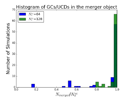
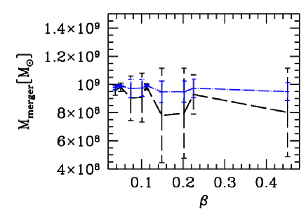
Figure 2: Left panel: Number of simulations vs. $N_{\rm merger}/N_{0}$ (total number of simulations is 162). Right Panel: Mass of the final object against the tidal filling parameter $\beta=5\cdot R_{\rm cc}/r_{\rm tidal}$. It is obvious that our parameter space produces tidally under-filling initial conditions and therefore almost all the mass of the CC ends up in the final object.

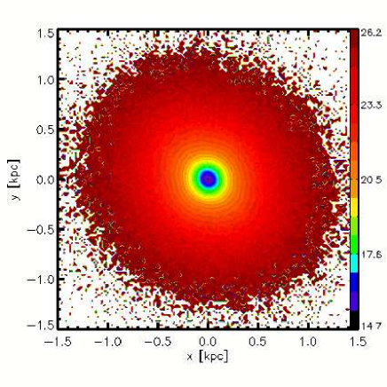
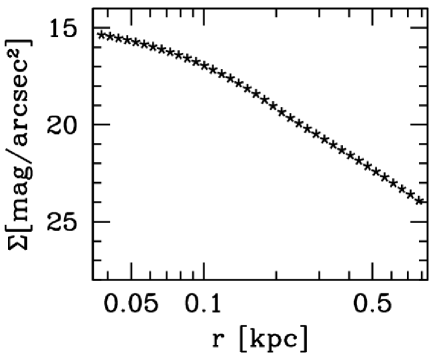
Figure 3: Sim85: $R_{\rm sc}=10$ pc, $R_{\rm cc}=50$ pc. Left panel: 2D pixel-map of surface brightness for one of our objects. The magnitudes are derived using a M/L-ratio of unity. Right panel: Radial profile of surface brightness calculated using concentric, logarithmically spaced rings.

We determine the number of constituents, which merge to build the final object $N_{\rm merger}$ and measure the final bound mass of this object $M_{\rm merger}$.

To obtain the effective radius $R_{\rm eff}$ of our object we fit a Sersic profile (Sersic, 1963) of the form

$$I(R) = I_{\rm e}\exp\left\{-b_{n}\left[\left(\frac{R}{R_{\rm eff}}\right)^{1/n}-1\right]\right\},$$ (3)

with $b_{n}$ satisfying the next equation which relates the incomplete Gamma function ($\gamma$) and the Gamma function ($\Gamma$)

$$\gamma(2n;b_{n}) = \frac{1}{2}\Gamma(2n).$$ (4)

The central surface brightness we determine by producing a 2D pixel-map of the surface densities of our object, searching for the pixel with the highest value and converting this value into magnitudes per arcseconds² by using a generic mass-to-light (M/L) ratio of unity. As we have no information in our simulations about age and metallicity of our stars (our particles are indeed rather phase-space representations), we refrain from applying any more realistic values for an old population.

The ellipticity of our object is taken from the routine Ellipse in IRAF. As input we use the 2D pixel map we already produced from our simulation results. We use the ellipticity of the nearest isophote to a generic distance of $100$ pc.

Finally, we use all particles in the central pixel to determine the central velocity dispersion of our object.

An overview of the combinations of setup parameters and the mean values of our results can be found in Tab. 3.

As Tab. 3 shows, we do not see any significant difference between the results obtained if we distribute the mass of the CC into $64$ objects or $128$. With this we do agree with previous studies (e.g. Brüns et al., 2009). Therefore, in order to boost our statistics we use in the following analysis of the results mean values obtained by adding the two sets of simulations together.

Furthermore, we see that almost all sets of parameters used in our study lead to objects similar to cEs. In Fig. 1 we compare our results with data from various observations in plotting total brightness against effective radius. Our simulations have effective radii similar to M32 and total masses similar to the mean value of compact ellipticals. Please note that we have used a generic M/L ratio of unity and therefore we overestimate the total luminosity of our objects. Furthermore, as we keep the mass of our CC constant and almost all SC/UCDs end up in the merger object, almost all of our results show approximately the same absolute magnitude.

3.1 SCs/UCDs in the merger object

In the left panel of Fig. 2 we show in how many simulations we obtain a certain fraction of star clusters/UCDs merging and ending up in the final object as a histogram. The blue bars represent simulations with $64$ constituents and the green bars $128$. It is clearly visible that in almost all simulations the majority if not all objects merge and build the final compact elliptical.

This behaviour can be understood well by looking at the right panel of Fig. 2. Here we show the final mass of the merger object as function of the tidal filling parameter $\beta$. For $\beta$ we use the definition from Fellhauer et al. (2002):

$$\beta = \frac{R_{\rm cut,cc}}{r_{\rm tidal}}$$ (5)

where $R_{\rm cut,cc}$ is the cut-off radius of the SC/UCD distribution, which is chosen to be $R_{\rm cut,cc}=5\cdot R_{\rm cc}$, and $r_{\rm tidal}$ is the tidal radius of this distribution at the given distance from the galaxy and for the used potential. The tidal radius is calculated using the standard equation from (Binney & Tremaine, 1987):

$$r_{\rm tidal} = \left(\frac{M_{\rm cc}=10^{9}{\rm M}_{\odot}}{3M_{\rm gal}(R_{\rm gal})}\right)^{1/3}R_{\rm gal}.$$ (6)

In our simulations the $\beta$ values are all below $0.5$. This means that all our initial models are extremely tidally under-filling. From this fact, it is clear that most constituents should end up in the final merger object. The old study by Fellhauer et al. (2002, , their figure 8) even showed that $\beta$ values slightly above unity still lead to almost all SCs merging.

In their figure 8 it is also shown that one might expect to see differences in this merging behaviour according to the filling factor parameter $\alpha$, which the authors define as:

$$\alpha = \frac{R_{\rm sc}}{R_{\rm cc}}.$$ (7)

The less filled the CC is with star clusters the lower should be the number of merged star clusters. We see this secondary trend in our simulations as well. The few simulations which have low $N_{\rm merger}$ values have also very low values of $\alpha$, i.e. these are mainly the simulations with $R_{\rm sc}=4$ pc and $R_{\rm cc}=100$ or $200$ pc.

According to Fellhauer et al. (2002) at low $\alpha$ values the small constituents are merging first with each other and only later build up the central merger object, while at higher values of $\alpha$ the merging happens fast and mainly with the central object.

Another mechanism to lose SCs from the CC is due to the random velocities they have. It is therefore possible that a SC is placed in the outskirts of the CC distribution with an outwards velocity, i.e. an apo-centre of its orbit beyond $R_{\rm cut,cc}$ and may have the possibility to escape.

With our choice of the initial mass of the CC, it is clear that the simulations with very incomplete merging processes, i.e. many escaping star clusters can not resemble a final object with properties of a compact elliptical, as the final mass is far below of what we expect of a cE.

3.2 Shapes

In Fig. 3 we show in the left panel a 2D smoothed pixel-map of one of our objects, which resembles a cE galaxy. We have converted the mass per area values of surface density from our simulation into magnitudes per solid angle using a generic mass-to-light ratio of unity. The figure shows clearly that the product of our simulation setup is a massive and compact object with a size and luminosity similar to what has been observed in compact elliptical galaxies.

In the right panel we show the radial surface brightness profile. The values are obtained by analysing the surface density of our merger object in concentric rings, which are logarithmically spaced. As most of our objects exhibit low ellipticities we are confident that the error by using rings instead of ellipses is of no significance.

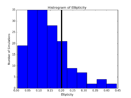
Figure 4: Histogram of the ellipticities of the final merger objects. The black line at $\epsilon=0.2$ denotes the commonly adopted value for cE galaxies. Most simulations exhibit objects with $\epsilon$ values below or equal to $0.2$, i.e. resemble the shape of most cE galaxies observed.

The ellipticity of an object is defined as

$$\epsilon = 1-\frac{b}{a}$$ (8)

where $a$ and $b$ are the semi-major and minor axis of an ellipse, respectively. The ellipticity of our objects is obtained from the function Ellipse in IRAF using the 2D pixel-maps (see e.g. left panel of Fig. 3) we compute. As ellipticities can change with radius, we use the ellipticity value of the isophote closest to $100$ pc.

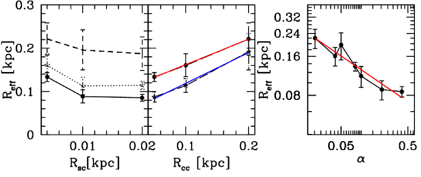
Figure 5: Effective radius $R_{\rm eff}$ of the merger objects. In the left panel we plot the effective radius as function of the size of the constituents $R_{\rm sc}$. Solid line connects simulations with $R_{\rm cc}=50$ pc, dotted line connects simulations with $R_{\rm cc}=100$ pc and dashed lines show $R_{\rm cc}=200$ pc simulations. We see that the final effective radius is almost independent of the choice of the size of the SCs. Only for very small SCs the effective radius is slightly higher but only within the error-bars. The middle panel shows $R_{\rm eff}$ as function of the distribution size $R_{\rm cc}$. The upper curve is from $R_{\rm sc}=4$ pc simulations and for the lower curve both $R_{\rm sc}$-values of $10$ and $20$ pc are used. In the right panel we plot $R_{\rm eff}$ against the filling factor parameter $\alpha$.

In the literature it is usually considered that compact ellipticals have no significant ellipticity (e.g. Chilingarian & Zolotukhin, 2015). The ellipticity of M32 is about E2 which means that the smaller axis is about 20% shorter than its larger axis. The exact ellipticity of M32 is 0.17 (Kent, 1987).

The ellipticity of the final object is not related to any of our simulation parameters ($R_{\rm gal}$, $R_{\rm sc}$ and $R_{\rm cc}$). In Fig. 4 one can see that almost all the simulations have ellipticities in the range of cEs, i.e. $\epsilon=0.2$ or less.

3.3 Effective radius of the final object (R_eff)

To obtain the effective radius $R_{\rm eff}$ of our final objects (after $10$ Gyr of evolution) we determine the radial surface brightness profile in logarithmically spaced concentric rings out to a maximum radius of $1.5$ kpc. As our objects exhibit low ellipticities (see Sect. 3.2), the use of rings instead of ellipses poses only small errors. We perform this calculation in all three main projections ($x-y$, $x-z$ and $y-z$) and calculate the mean values to avoid chance alignments. These mean values are now fitted using a Sersic profile as described in Eq. 3.

In our simulations we see no dependency of $R_{\rm eff}$ with the choice of the galactic distance of our cluster complex. Again, this can be explained by the fact that all our models are initially tidally under-filling and therefore the gravitational pull of the galactic potential has no or only very small influence on the formation and evolution of the merger object. Therefore, we can neglect the galactic distance in the following analysis and bin all simulations with the same internal parameters independent of their distance to the galaxy to obtain better statistics.

The same is true if we compare simulations with $N_{0}=64$ and $128$. As most of the SCs/UCDs in the CC merge to build the final object, its internal parameters are only marginally dependent on the initial number of constituents and we are able to increase the statistical significance of our results further by binning the simulations independent of their initial $N_{0}$ as well.

In Fig. 5 we show the resulting effective radius as function of the remaining parameters $R_{\rm sc}$, $R_{\rm cc}$ and their combination, i.e. the filling factor $\alpha$. The left panel shows $R_{\rm eff}$ as function of $R_{\rm sc}$. We see a slight trend that with a larger size of the constituents we obtain merger objects which are more concentrated. But this trend is well within the calculated $1\sigma$ error-bars. Especially, between $R_{\rm sc}=10$ pc and $20$ pc we see no significant difference any longer. This means, as long as we build our merger object out of extended constituents, their size does not influence the scale radius of the final object. Only if concentrated initial SCs are used then we may see a slower merging process (see Fellhauer et al., 2002, for a more detailed explanation) and a more extended final object.

The middle panel of Fig. 5 shows only two different lines as we choose to bin the simulations with $R_{\rm sc}=10$ and $20$ pc here (top line shows $R_{\rm sc}=4$ pc results, bottom line $R_{\rm sc}=10$ and $20$ pc). A very clear linear trend is visible that with a larger size of the distribution, we see a larger final object. We fit a line to the results and obtain as slope $0.59\pm 0.01$ for $R_{\rm sc}=4$ pc, shown as the red line and $0.71\pm 0.06$ for the other results (blue line). As we focus more on simulations with extended initial objects we can give the following relation as a rule by thumb:

$$R_{\rm eff} \approx 0.7\cdot R_{\rm cc}.$$ (9)

Finally, in the right panel we show the dependence of our results on the ratio of both input parameters: $\alpha$ (see Eq. 7). In the double-logarithmic plot the results of our simulations follow a linear trend, i.e. a power law dependence. If we fit a power-law to our results we get $-0.35\pm 0.05$ as power-law index, i.e. we can write:

$$R_{\rm eff} \propto \alpha^{-1/3}.$$ (10)

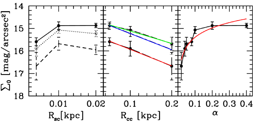
Figure 6: Central Surface Brightness $\Sigma_{0}$. In the left panel we show the central surface brightness as function of the size of the constituents $R_{\rm sc}$. The lines are the same as in Fig. 5. The middle panel shows $\Sigma_{0}$ as function of the size of the distribution $R_{\rm cc}$. Bottom line (red) is for $R_{\rm sc}=4$ pc, middle line (blue) for $R_{\rm sc}=10$ pc and top line (green) for $R_{\rm sc}=20$ pc. In the right panel we plot $\Sigma_{0}$ as function of the filling factor $\alpha$.

This result implies that a larger ’filling factor’ $\alpha$ leads to more compact merger objects. An explanation could be deduced when compared to the results found in Fellhauer et al. (2002). There, larger values of $\alpha$ lead to a change in the merging behaviour, i.e. the SCs rather merged with the fast growing central object. If $\alpha$ is low then the constituents rather merge with each other first and the central merger object appeared later. As a merger between two objects (dry merger - without gas) always leads to a more extended object than the two initial ones, the above mentioned change in merging behaviour can explain that we find more compact merger objects when starting with less compact objects to begin with. Here the initial constituents form first very extended secondary objects, which then merge and build an even more extended central object.

Comparing the results to the quoted effective radii for compact ellipticals in the literature, which ranges between $80$ and $200$ pc, only the simulations with the smallest scale-length for the constituents ($R_{\rm sc}=4$ pc) together with the largest size of the cluster complex distribution ($R_{\rm cc}=200$ pc) are just outside this window (see left panel of Fig. 5). This points into the direction that, to obtain cEs (at least in this formation scenario), we need compact, massive CCs with extended objects to have a fast and efficient merger process. Therefore, we need the merging of UCD-like objects to form a cE rather than compact SCs.

3.4 Central Surface Brightness ($\Sigma_{0}$)

In this section we present the results of the central surface brightness $\Sigma_{0}$ of our merger objects. As explained before we construct smoothed 2D pixel maps of our objects with their surface density measured in M_⊙ pc^-2. These values we convert into mag. arcsec^-2 using a generic mass-to-light ratio of unity. As magnitudes are a logarithmic scale, a factor of a few, obtained by using your favourite pass-band and a mass-to-light ratio for a mainly old population in that exact band, will alter our results only marginally, in extreme cases to about one magnitude fainter.

Once the 2D map is constructed, we use the brightest, central pixel to deduce the central surface brightness of our objects. As our pixel size is $20$ pc, our models have a higher resolution as most observations of distant cEs could obtain. This could lead to another source of higher values of $\Sigma_{0}$ deduced from our simulations than actually observed.

The values reported in Tab. 3 with their errors are obtained by taking a mean value from the three simulations with the same parameters but different random realisations.

Looking at the results, no dependency on the distance $R_{\rm gal}$ to the centre of the galaxy is visible. The explanation is the same as for the effective radii, our models are all tidally under-filling at the beginning and the gravitational forces of the host galaxy are of rather minor importance. Furthermore, as in the previous section we do not see any strong dependence on the number of initial objects $N_{0}$. We are therefore able to use all simulations independent of $R_{\rm gal}$ and $N_{0}$ to calculate the mean values and errors, increasing the statistical base.

In Fig. 6 we show the central surface brightness of the merger objects as function of the same initial parameters as in Fig. 5 and we see exactly the same trend as with the effective radius. For very small ($R_{\rm sc}=4$ pc) constituents we get more extended objects with lower central brightnesses as for the more extended initial objects ($R_{\rm sc}=10$ and $20$ pc), which again do not differ significantly (left panel). The dashed line shows the results for $R_{\rm cc}=50$ pc, the dotted line shows $R_{\rm cc}=100$ pc results and finally the solid line represents $R_{\rm cc}=200$ pc.

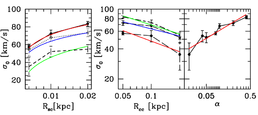
Figure 7: Central velocity dispersion $\sigma_{0}$. Left panel: Central velocity dispersion as function of $R_{\rm sc}$. Middle panel: $\sigma_{0}$ as function of $R_{\rm cc}$. Right panel: $\sigma_{0}$ as function of $\alpha$. Lines are the same as in Fig. 6.

The middle panel also shows the same trend as before: larger initial distributions form less concentrated merger objects which in turn have lower central brightnesses.

The central surface brightness correlates linearly with the size of the CC. The slopes of the fitting curves are $7.3\pm 0.4$, $5.5\pm 0.6$ and $7.19\pm 0.02$ for $R_{\rm sc}=4$ (red curve), $10$ (blue) and $20$ pc (green) respectively ($R_{\rm cc}$ measured in kpc).

The right panel again shows the surface brightness as function of the parameter $\alpha$. The trend is as expected that with larger alphas we obtain brighter, i.e. more concentrated, objects. In contrast to $R_{\rm eff}$, which seems to decrease further with $\alpha$, here there might be a trend to a kind of maximum central luminosity of about $14.9$ mag arcsec^-2. If there is an equivalent minimal effective radius at higher $\alpha$ values as probed in this study here, remains open. This has to be investigated in a possible follow up of this study.

Fitting a power law to the results we obtain that

$$\Sigma_{0} \propto \alpha^{-0.039\pm 0.007}.$$ (11)

The surface brightness of known cEs ranges approximately from $14$ to $20$ mag arcsec^-2 (see table 1 in Chilingarian et al., 2007) (table 2 in Huxor et al., 2013). In that sense all of our simulations match the observational constraints found for cE galaxies.

3.5 Central Velocity Dispersion ($\sigma_{0}$)

In this section we focus on the dynamics of the merger objects. As a benchmark to compare our results with observations we use the central velocity dispersion $\sigma_{0}$ of our models. The value is obtained summing all line-of-sight velocities of the particles located in the densest pixel, we use to determine the central surface brightness.

Tab. 3 shows that the results again do not depend on the distance to the galaxy $R_{\rm gal}$ and the used number of SCs $N_{0}$ and we are able to group simulations only differing by these parameters together.

In Fig. 7 we show the dependency of $\sigma_{0}$ on the parameters $R_{\rm sc}$ (left panel), $R_{\rm cc}$ (middle panel) and the combination of the two parameters $\alpha$ (right panel). Colours and lines are the same as in Fig. 6.

We see a straightforward trend, which is expected, taking the previous results into account. As the final mass of our cEs is approximately the same, the velocity dispersion should depend on the size of the object only, i.e. more concentrated, smaller objects should exhibit larger velocity dispersion. Exactly this is visible in our results. As explained before, smaller constituents lead to a slower merging and more extended objects and therefore exhibit lower velocity dispersions, i.e. $R_{\rm sc}$ and $\sigma_{0}$ are correlated. On the contrary, larger distributions lead to larger objects and henceforth to small velocity dispersions, the two quantities are anti-correlated.

The fitting lines shown in the figures are power-laws. In the middle panel we obtain the following exponents for the decrease: $-0.4\pm 0.2$, $-0.24\pm 0.08$ and $-0.30\pm 0.07$ for the different choices of $R_{\rm sc}=20$, $10$ and $4$ pc respectively. As we have found a close to linear dependency of $R_{\rm eff}$ on $R_{\rm cc}$ we would expect from simple stellar dynamical arguments (virial equilibrium)

$$\sigma \sim R_{\rm cc}^{-0.5}.$$

We see this relation only holds if we start with large enough constituents, i.e. UCD-like objects.

In the right panel we show how $\sigma_{0}$ varies with $\alpha$. As $\alpha$ is proportional to $R_{\rm sc}$ and anti-proportional to $R_{\rm cc}$ we expect that $\sigma_{0}$ should have a strong correlation with $\alpha$. A power-law fitted to the results gives a slope of $0.26\pm 0.04$ and so we could approximately write

$$\sigma_{0} \propto \alpha^{1/4}.$$ (12)

The range in observed velocity dispersions in cE galaxies is rather large. In their table 2 Ferré-Mateu et al. (2017) report for NGC 2970 $47.7\pm 1.6$ km s^-1 and for PSC012519 a value of $222\pm 2.3$ km s^-1. The central velocity dispersion of M32 is reported in van der Marel et al. (1998) to be $76\pm 10$ km s^-1.

If we pose a minimum velocity dispersion of $40$ km s^-1 to call a merger object a cE galaxy, we see that all our simulations except the parameter combination of $R=4$ pc and $R_{\rm cc}=200$ pc are reproducing objects with velocity dispersions similar to cE galaxies. Again only the parameter set which leads to a slow merging process is not able to reproduce the necessary values for cEs.

4 Discussion and Conclusions

We perform simulations in the merging star cluster scenario using a very high total mass of $10^{9}$ M_⊙ for the cluster complex. The merging star cluster scenario is successful in reproducing the formation of extended star clusters and UCDs. With the chosen high total mass, which is an order of magnitude higher than used for the formation of massive UCDs we want to open up a new formation scenario for compact ellipticals like M32. We argue that in the early, more gas-rich Universe we might have stronger star burst events as seen today in interacting galaxies, which might lead to the formation of a compact star forming region, i.e. a cluster complex, producing $10^{9}$ M_⊙ in star clusters, forming a bound entity.

In the present Universe we do see recently formed UCD-like objects with luminous and dynamical masses of $10^{8}$ M_⊙. As an example we point to W3 in NGC 7252 (Maraston et al., 2004). At an age of $300$ to $500$ Myr this UCD-like object is not formed through any stripping or other destructive channel. It has the age of the interaction of the merger remnant of the host system and therefore was formed in a star-formation burst during the interaction. As star-formation is believed to be higher in the past (e.g. Shibuya et al., 2016; Tacchella et al., 2018), we think it is reasonable to assume that CCs with masses similar to cEs could have formed.

Renaud et al. (2015) pointed out that in their simulations of interacting galaxies the most massive star-forming regions are found close to the centre of the merging pair, i.e. making these massive objects ideal candidates to sink to the centre due to dynamical friction, while Duc et al. (2000) find observational evidence of tidal dwarf galaxies at the tip of the tidal tails with masses exceeding $10^{9}$ M_⊙.

Fellhauer & Kroupa (2005) reported about the observability of the merging star cluster formation scenario. As this scenario is a very rapid process, the authors concluded that only if W3 in NGC 7252 is at its lower age limit ($300$ Myr), there might be a chance to observe the final stages of the ongoing merging process. At the higher age limit ($500$ Myr) the merging process is over and the object is dynamically indistinguishable from other formation scenarios. Therefore, for old objects like M32 we do not expect to find any dynamical tracer of its formation process any longer, which would confirm our scenario.

Some groups argue that the presence of tidal tails associated with UCDs are a clear sign of a past stripping process but Brüns et al. (2009) report similar tails in the merging star cluster scenario. The presence or absence of a massive black hole in the centre could be a hint of a more massive galaxy origin. Indeed, Voggel et al. (e.g. 2018) found massive black holes in UCDs around Centaurus A, making them excellent candidates for a more massive galaxy origin. These high resolution observations are still ongoing but for every positive detection there is also a non-detection in a similar UCD present.

All the presented evidence makes it likely that objects like UCDs are not from a single formation channel but actually a mixed bag of objects.

As we have argued with examples of the less-massive UCDs, we think that the same line of reasoning can be applied to compact ellipticals as well.

There is one thing which our simple stellar dynamical models cannot reproduce. Observing M32 Monachesi et al. (2012) found two different stellar populations:

• $\sim 40\pm 17$% of the mass in a 2-5 Gyr old, metal-rich population ([M/H]$=0.02\pm 0.01$ dex)

• $\sim 55\pm 21$% of the total mass in stars older than 5 Gyr, with slightly subsolar metallicities.

Our simulations do not treat metallicities and and gas is not included in our simulations. We would speculate that, when forming a cluster complex that massive, the expelled gas, seen e.g. as H-alpha bubbles around the CCs in the Antennae (e.g. Whitmore et al., 1999), stays bound to the forming merger object and is able to fall back in, forming at least a second generation of stars.

In Alarcon Jara et al. (2018) we have shown in a different project, that our results and conclusions do not change when adopting a star formation history into our models. So, we are confident that in this scenario an included star formation history would also show no major differences.

Every simulation performed in this study leads to a final bound object in which the majority of star cluster have merged. We analyse the resulting object and are determining its shape, mass, effective radius, central surface brightness and central velocity dispersion. These values are compared with observational values of compact ellipticals found in the literature.

The main result of this study is, that indeed it is possible to obtain a cE galaxy in the merging star cluster scenario, matching all the above mentioned observables.

Furthermore, we established the following relations:

• The effective radius of the final object is inversely proportional to the size of the used star clusters. This result seems at first counter-intuitive as dry merger processes, as happening here in this study, are always increasing the effective radius.

  The reason for this anti-correlation is in the different merging behaviour we find for different choices of parameters. Defining a ’filling factor’ $\alpha=R_{\rm sc}/R_{\rm cc}$, low values of $\alpha$, i.e. using small, compact star clusters, lead to the merging of pairs of star clusters throughout the cluster complex first, before finally a central object is built up. This object now has a larger scale radius.

  In the case of large filling factors, the merging process is very fast and directly with the forming central object. This results in more compact objects.

• The effective radius is linearly proportional to the used size of the cluster complex. As a rule-by-thumb we give $R_{\rm eff}=0.7R_{\rm cc}$.

• With our studied parameter range, the obtained effective radii are between $90$ and $260$ pc, which marks the range of cE galaxies.

• The range of ellipticities $\epsilon$ is between $0.05$ and $0.32$, with almost all simulations having ellipticities in the range of cEs ($\epsilon\leq 0.2$).

• We always obtain central surface brightnesses which are matching the values of cEs.

• The merger objects exhibit velocity dispersions in the range of about $50$ to $80$ km s^-1, thereby matching the observational values. We have in total three simulations in which the final velocity dispersion is too low to match cEs. These simulations correspond to incomplete merging (many star clusters avoid the merging process and fly away) and have to be ruled out by showing a final mass which is too low anyway. All of these three simulations have $R_{\rm sc}=4$ pc and $R_{\rm cc}=200$ pc, i.e. $\alpha=0.02$.

These results point to the fact that in order to obtain an object similar to a cE galaxy, it is more favourable to have a cluster complex with a high filling factor, i.e. either small extension or extended objects forming within.

The merging star cluster scenario is not the only way to produce a cE galaxy. Other theories for the formation of cEs include the tidal stripping and truncation scenario (Faber, 1973) either with an elliptical galaxy with a dense core as origin (e.g. Faber, 1973) or the bulge of a partially stripped disc galaxy (e.g. Bekki et al., 2001). Or cEs could also have an intrinsic origin and are the natural extension of the class of elliptical galaxies to smaller sizes and lower luminosities (Wirth & Gallagher, 1984; Kormendy et al., 2009).

Nevertheless, our scenario opens up a new possible formation channel to explain the existence of compact elliptical galaxies.

Acknowledgments: FUZ, MF, AGAJ, DRMC and CAA acknowledge funding through Fondecyt Regular No. 1180291 and BASAL Centro de Astrofisica y Tecnologias Afines (CATA) AFB-170002. MF acknowledges funding through the Concurso Proyectos Internacionales de Investigacion No. PII20150171. AGAJ acknowledges financial support from Carnegie Observatories through the Carnegie-Chile fellowship.

References

- Alarcon Jara et al. (2018) Alarcón Jara, A.G.; Fellhauer, M.; Matus Carrillo, D.R.; Assmann, P.; Urrutia Zapata, F.; Hazeldine, J.; Aravena, C.A. 2018, MNRAS, 473, 5015
- Bastian et al. (2005) Bastian N., Gieles M., Efremov Y.N., Lamers H.J.G.L.M. 2005, A&A, 443, 79
- Bekki et al. (2001) Bekki, K.; Couch, W.J.; Drinkwater, M.J.; Gregg, M.D. 2001, ApJ, 557, 39
- Binney & Tremaine (1987) Binney, J.; Tremaine S. 1987, ’Galactic Dynamics’, Princton University Press
- Brodie & Larsen (2002) Brodie, J.P.; Larsen, S.S. 2002, AJ, 124, 1410
- Brüns et al. (2009) Brüns, R.C.; Kroupa, P.; Fellhauer, M. 2009, ApJ, 702, 1268
- Brüns et al. (2011) Brüns, R.C.; Kroupa, P.; Fellhauer, M.; Metz, M.; Assmann, P. 2011, A&A, 529, 138
- Brüns & Kroupa (2012) Brüns, R.C.; Kroupa, P. 2012, A&A, 547, 65
- Burkert et al. (2005) Burkert, A.; Brodie, J.; Larsen, S. 2005, ApJ, 628, 231
- Chandar et al. (2004) Chandar, R.; Whitmore, B.; Lee, M.G. 2004, ApJ, 611, 220
- Chilingarian et al. (2007) Chilingarian, I.; Cayatte, V.; Chemin, L.; Durret, F.; Laganá, T. F.; Adami, C.; Slezak, E. 2007, A&A, 466, 21
- Chilingarian et al. (2009) Chilingarian, I.; Cayatte, V.; Revaz, Y.; Dodonov, S.; Durand, D.; Durret, F.; Micol, A.; Slezak, E. 2009, Science, 326, 1379
- Chilingarian & Zolotukhin (2015) Chilingarian, I.; Zolotukhin, I. 2015, Science, 348, 418
- Drinkwater et al. (2000) Drinkwater, M.J.; Jones, J.B.; Gregg, M.D.; Phillipps, S. 2000, PASA, 17, 227
- Du et al. (2018) Du, M.; et al. 2018, ApJ submitted; arXiv:1811.06778
- Duc et al. (2000) Duc, P.-A.; Brinks, E.; Springel, V.; Pichardo, B.; Weilbacher, P.; Mirabel, I. F. 2000, AJ, 120, 1238
- Faber (1973) Faber, S.M. 1973, ApJ, 179, 423
- Fellhauer et al. (2000) Fellhauer, M.; Kroupa, P.; Baumgardt, H.; Bien, R.; Boily, C.M.; Spurzem, R.; Wassmer, N. 2000, NewA, 5, 305
- Fellhauer et al. (2002) Fellhauer, M.; Baumgardt, H.; Kroupa, P.; Spurzem, R. 2002, CeMDA, 82, 113