OV] $\lambda\lambda$1213.8,1218.3 emission from extended nebulae around quasars: contamination of Ly$\alpha$ and a new diagnostic for AGN activity in Ly$\alpha$-emitters

Abstract

We investigate the potential for the emission lines OV] $\lambda\lambda$1213.8,1218.3 and HeII $\lambda$1215.1 to contaminate flux measurements of Ly$\alpha$ $\lambda$1215.7 in the extended nebulae of quasars. We have computed a grid of photoionization models with a substantial range in the slope of the ionizing powerlaw (-1.5 $<$ $\alpha$ $<$ -0.5), gas metallicity (0.01 $<$ $Z/Z_{\odot}$ $<$ 3.0), gas density (1 $<$ $n_{H}$ $<$ 10⁴ cm^-3), and ionization parameter (10^-5 $<$ U $<$ 1.0). We find the contribution from HeII $\lambda$1215.1 to be negligible, i.e., $<$ 0.1 of Ly$\alpha$ flux, across our entire model grid. The contribution from OV] $\lambda\lambda$1213.8,1218.3 is generally negligible when U is low ($\la$10^-3) and/or when the gas metallicity is low ($Z/Z_{\odot}$ $\la$ 0.1). However, at higher values of U and Z we find that OV] can significantly contaminate Ly$\alpha$, in some circumstances accounting for more than half the total flux of the Ly$\alpha$+HeII+OV] blend. We also provide means to estimate the fluxes of OV] $\lambda\lambda$1213.8,1218.3 and HeII $\lambda$1215.1 by extrapolating from other lines. We estimate the fluxes of OV] and HeII for a sample of 107 Type 2 active galaxies at z$>$2, and find evidence for significant ($\geq$10%) contamination of Ly$\alpha$ fluxes in the majority of cases (84%). We also discuss prospects for using OV] $\lambda\lambda$1213.8,1218.3 as a diagnostic for the presence of AGN activity in high-z Ly$\alpha$ emitters, and caution that the presence of significant OV] emission could impact the apparent kinematics of Ly$\alpha$, potentially mimicking the presence of high-velocity gas outflows.

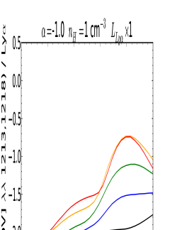
Figure 1: Cross-cuts through our grid of ionization-bounded (optically-thick) photoionization model grid, showing HeII+OV] / Ly$\alpha$ vs U curves for different fixed values of gas metallicity, $\alpha$ and $n_{H}$. In Figs. 1-6, the multiplicative transmission factor of Ly$\alpha$ ($\leq$1) is shown above each panel.

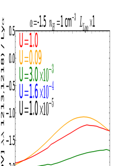
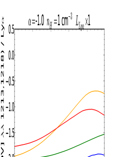
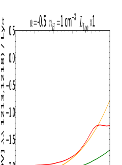
Figure 2: Similar to Fig.  1, but showing HeII+OV] / Ly$\alpha$ vs. metallicity curves for different fixed values of U, $\alpha$ and $n_{H}$.

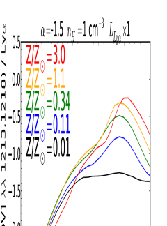
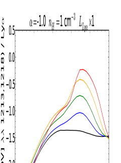
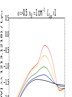
Figure 3: Cross-cuts through our grid of matter-bounded (optically-thin) photoionization model grid, showing HeII+OV] / Ly$\alpha$ vs U curves for different fixed values of gas metallicity, $\alpha$ and $n_{H}$.

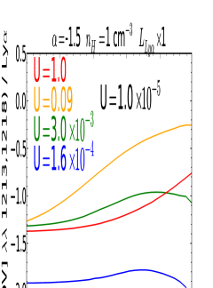
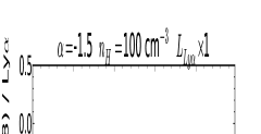
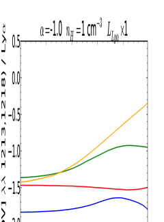
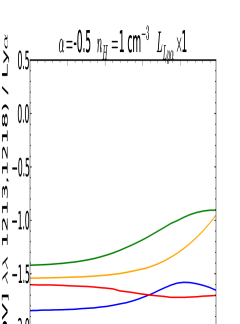
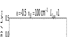
Figure 4: Similar to Fig.  3, but showing HeII+OV] / Ly$\alpha$ vs. metallicity curves for different fixed values of U, $\alpha$ and $n_{H}$.

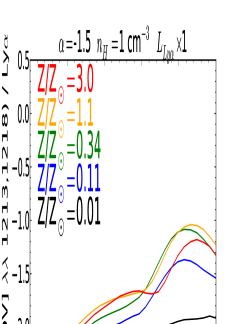
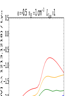
Figure 5: The impact of Ly$\alpha$ absorption on the HeII+OV] / Ly$\alpha$ vs U curves for ionization-bounded (optically-thick) photoionization models. The presence of Ly$\alpha$ absorption has been simulated by multiplying the Ly$\alpha$ luminosity by 1.0 (no absorption, top row), 0.2 (middle row) or 0.5 (bottom row). Due to the fact that gas densities of 1, 100 and 10,000 cm^-3 give essentially identical results, here we show only the subset of our grid that uses $n_{H}$=1 cm^-3.

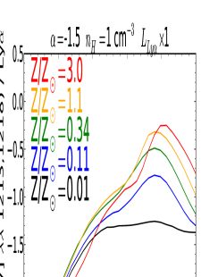
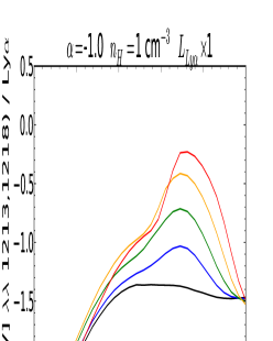
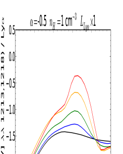
Figure 6: The impact of our simple Ly$\alpha$ absorption model on the HeII+OV] / Ly$\alpha$ vs U curves for matter-bounded (optically-thin) photoionization models. The presence of Ly$\alpha$ absorption has been simulated by multiplying the Ly$\alpha$ luminosity by 1.0 (no absorption, top row), 0.2 (middle row) or 0.5 (bottom row). Due to the fact that gas densities of 1, 100 and 10,000 cm^-3 give essentially identical results, here we show only the subset of our grid that uses $n_{H}$=1 cm^-3.

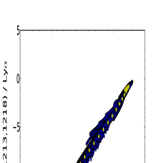
Figure 7: Log OV]/Ly$\alpha$ vs. log NV/Ly$\alpha$, [NeV]/Ly$\alpha$, OVI/Ly$\alpha$, and CIV/Ly$\alpha$. Every photoionization model from our grid is plotted (blue circles), with the exception of models that include absorption of Ly$\alpha$ by a HI screen, which are not shown here. All combinations of gas metallicity, density, U and $\alpha$ used in our grid are represened in these plots. Our ionization-bounded model sequence with $Z/Z_{\odot}$=1.1, $\alpha$=-1.0, and $n_{H}$=100 cm^-3 is highlighted using yellow circles – as described in the text, we use this subset of our grid to obtain an extrapolation of the expected OV] flux from NV, [NeV], OVI and CIV.

1 Introduction

The HI Ly$\alpha$ emission line at 1215.7 Å is among the brightest lines in the ultraviolet spectra of active galaxies, and remains one of the principal means to detect and study extended gaseous material around quasars in the distant Universe (e.g. Villar-Martín et al. 2002; Weidinger, Møller & Fynbo 2004; Christensen et al. 2006; Borisova et al. 2016).

The study of the distribution and dynamics of extended envelopes of gas around active galaxies at high redshift now makes extensive use of the Ly$\alpha$ emission line, in order to examine key processes such as feedback activity and accretion of cold gas (e.g. Vernet et al. 2017: Silva et al. 2018a; Arrigoni Battaia et al. 2018; Dors et al. 2018). As such, it is crucial to understand the physics of the production and radiative transfer of this emission line.

One of the main channels for production of Ly$\alpha$ emission in quasar nebulae is recombination fluorescence, where ultraviolet photons emitted by the accretion disc of the quasar photoionize hydrogen, leading to emission of a line and continuum spectrum upon recombination (e.g. Heckman et al. 1991). As a resonant line, Ly$\alpha$ can also be subject to absorption and transfer effects that, in some circumstances, can significantly alter its observed kinematics and flux (e.g. Villar-Martín, Binette & Fosbury 1996; Dijkstra, Haiman & Spaans 2006). In addition, collisional excitation can, under certain circumstances, make a significant contribution to the production of Ly$\alpha$ photons (e.g. Villar-Martín et al. 2007a), possibly even becoming the dominant channel of Ly$\alpha$ production at low gas metallicities (Humphrey et al. 2018).

A further possible complication is the presence of additional emission lines very close to the wavelength of Ly$\alpha$, namely, the non-resonant recombination line HeII $\lambda$1215.1, and the semi-forbidden doublet OV] $\lambda\lambda$1213.8,1218.4. Clearly, it is important to understand whether, and to what extent the measured fluxes of Ly$\alpha$ are enhanced by the presence of HeII $\lambda$1215.1 and OV] $\lambda\lambda$1213.8,1218.4. This issue was discussed in the context of the high-density ($n_{H}\ga$10⁶ cm^-3) broad-line region (BLR) of quasars by Shields et al. (1995), who found that the contribution from HeII and OV] can become non-negligible in the case of highly-ionized, optically-thin BLR clouds, with flux ratios of up to OV]/Ly$\alpha$$\sim$1 and HeII $\lambda$1215.1/Ly$\alpha$$\sim$0.2 being reached in their model grid (see also Ferland et al. 1992). However, we are not aware of any previous photoionization calculations for the lower-density, narrow-line emitting region (NLR) or Ly$\alpha$ halo that considers the possible contamination of the Ly$\alpha$ flux from these lines. Addressing this question for the NLR and Ly$\alpha$ halo of AGN is the main focus of this work.

In a previous paper, we applied the modelling code Mappings 1e (Binette, Dopita & Tuohy 1985; Ferruit et al. 1997; Binette et al. 2012) to model the combined effects of several mechanisms to enhance Ly$\alpha$ emission from AGN-photoionized nebulae at high redshift (Humphrey et al. 2018). Here we present a follow-up study to quantify the potential contamination from HeII and OV] emission to flux measurements of Ly$\alpha$ in low density, narrow-line nebulae that are photoionized by an AGN.

2 Photoionization models

Our objective is to simulate the ionization/excitation conditions in spatially extended, low density gas that is being photoionized by a central AGN, such as the NLR (e.g. Pogge 1988) or Ly$\alpha$ halo (e.g. Reuland et al. 2003). We have used the multi-purpose modeling code MAPPINGS 1e (Binette, Dopita & Tuohy 1985; Ferruit et al. 1997; Binette et al. 2012) to compute our grid of AGN photoionization models.

Our grid consists of 16200 individual photoionization models, each one representing an ionized cloud with a specific set of physical and ionization properties. Our models consist of a plane-parallel slab of gas which is illuminated by a powerlaw of the form $S_{\nu}\propto\nu^{\alpha}$, where $\alpha$ is the spectral index, $\nu$ is emission frequency and $S_{\nu}$ is flux density. As a starting point from which to define non-Solar gas chemical abundances, we adopt the Solar abundance set of Asplund et al. (2006). To vary gas metallicity, we start from the Solar abundance set, and we then scale all metals linearly such that $Z/Z_{\odot}$ $\propto$ O/H, except in the case of nitrogen, for which we take into account secondary production (e.g. Henry et al. 2000) by assuming N/O $\propto$ O/H for $Z/Z_{\odot}>$ 0.3 and N/H $\propto$ O/H for $Z/Z_{\odot}<$ 0.3.

For three different values of hydrogen gas density ($n_{H}$ = 1, 100, 10⁴ cm^-3), three different ionizing power law indices ($\alpha$=-1.5, -1.0 or -0.5) and two optical depth regimes (thick or thin), we computed 30$\times$30 sub-grids of 900 models with 30 values of ionization parameter U (10^-5–1.0) and 30 values of gas metallicity $Z/Z_{\odot}$ (0.01–3.0).

Our optically thick models adopt the ionization-bounded model termination, which ends the calculation when the ionization fraction of hydrogen has fallen below 0.01. This simulates a cloud which absorbs essentially all the ionizing photons from the incident spectrum, with the exception of some photons at the high-energy end of the spectrum and, in some circumstances, UV photons at $hv<$13.6 eV that ionize some neutral metal species (e.g., C, S, Si, etc.).

In the case of our optically thin models, the calculation terminates when the fraction of absorbed H-ionizing photons (by number) reaches 0.05, resulting in a Lyman-continuum-leaking, matter-bounded cloud. This corresponds to a cloud that is insufficiently optically thick to absorb all of the ionizing EUV photons, so that some of these photons pass through unabsorbed to escape from the rear of the cloud.

The Ly$\alpha$ emission line of Type II active galaxies and Ly$\alpha$ blobs sometimes show strong, narrow absorption features due to associated, intervening HI stuctures (e.g. van Ojik et al. 1997; Wilman et al. 2004, 2005), or unusually low Ly$\alpha$/HeII flux ratios suggestive of partially absorbed Ly$\alpha$ (e.g. van Ojik et al. 2004). To simulate the effect of absorption on Ly$\alpha$ by an external HI screen, we have multiplied the Ly$\alpha$ luminosity by a transmission factor of 0.5 (strong absorption), 0.8 (moderate absorption) or 1.0 (no absorption). It is non-trivial to convert these values into neutral hydrogen column density $N_{HI}$, because the transmission factor also depends on the kinematic width and covering factor of the absorbing gas, and the kinematic properties of the Ly$\alpha$ emitting gas. Nevertheless, for the Ly$\alpha$ flux to be significantly reduced, an HI column density of $N_{HI}\ga$ 10¹⁴ cm^-2 would be required. (See e.g. Silva et al. 2018a for a more detailed discussion of the degeneracies involved in recovering $N_{HI}$ from the Ly$\alpha$ velocity profiles of quasars.) In the interest of simplicity, we assume that the HI absorption (if present) is positioned near the centre of the Ly$\alpha$ emission line and thus does not absorb any of the HeII $\lambda$1215.1 or OV] $\lambda\lambda$1213.8,1218.4 emission.

We emphasize that our treatment of HI absorption is, strictly speaking, valid only for the simple case of absorption of Ly$\alpha$ by an external HI screen that produces a narrow absorption feature centred on or near the peak of the Ly$\alpha$ emission. More complex HI geometries, such as multiple HI absorption systems offset from the centre of the Ly$\alpha$ emission line, or absorption and destruction of Ly$\alpha$ photons in situ within the emitting gas, may produce significantly different results. However, a detailed treatment of other (more complex) HI absorpion geometries is beyond the scope of this paper.

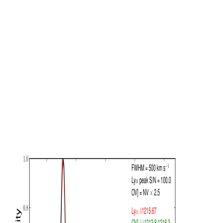
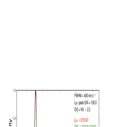
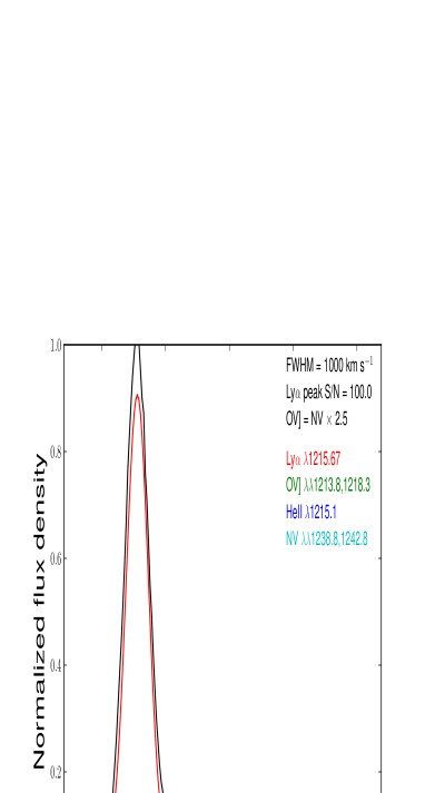
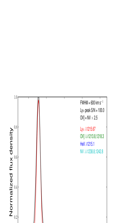
Figure 8: Model spectra for the NLR or Ly$\alpha$ halo of active galaxies, for different values of line FWHM. The emission lines shown are Ly$\alpha$ (red), HeII $\lambda$1215.1 (blue), OV] $\lambda\lambda$1213.8,1218.3 (green) and NV $\lambda\lambda$1238.8,1242.8 (cyan). The black line shows the sum of the emission lines, plus a flat continuum component containing Gaussian noise. As discussed in the text, the detectability of OV] depends strongly on the FWHM of the line emission. When the FWHM is large (e.g., 1000 km s^-1), OV] and Ly$\alpha$ are blended to such an extent that the velocity profile shows no discernable sign of the presence of the OV] lines (top left). At FWHM$\sim$500-600 km s^-1 (top right and centre left), the presence of OV] $\lambda$1218.3 becomes apparent as small excess of flux in the red wing of the Ly$\alpha$ profile. When FWHM $\la$400 km s^-1 (centre right and bottom panels), OV] $\lambda$1218.3 is resolved from Ly$\alpha$. The blue component of the OV] doublet (OV] $\lambda$1218.3) becomes discernable at FWHM$\sim$300 km s^-1 (bottom left), and is fully resolved from Ly$\alpha$ at FWHM$\la$200 km s^-1. Note that HeII $\lambda$1215.1 remains blended with Ly$\alpha$ in all the model spectra considered here.

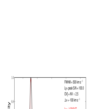
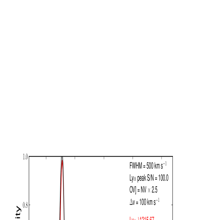
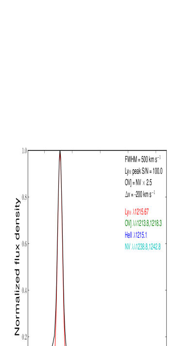
Figure 9: Model spectra for the NLR or Ly$\alpha$ halo of active galaxies, for FWHM=500 km s^-1, with the high-ionization lines shifted from Ly$\alpha$ by -300, -200, -100, 100, 200 and 300 km s^-1. Lines have the same meaning as in Fig.  8.

3 Model Results

3.1 Optically Thick Models

In this section we describe the behaviour of the fluxes of HeII and OV] relative to that of Ly$\alpha$ in our optically-thick photoionization models. We quantify the contribution of HeII and OV] to the Ly$\alpha$+HeII+OV] blend using log HeII+OV] / Ly$\alpha$. In Figures  1 and  2 we illustrate the behaviour of this ratio for cross-cuts along the $U$ or $Z/Z_{\odot}$ axis of our grid. The results described in this subsection are principally derived from Fig.  1, with Fig.  2 providing an additional, supplementary view.

Starting at the low $U$ end of our grid (log $U=$-5), the contribution from HeII and OV] is negligible, with log HeII+OV] / Ly$\alpha$ $\la$-2.5. As $U$ increases, the contribution from HeII grows until it reaches a plateau at log $U\ga$-3. However, even at its maximum flux ratio with Ly$\alpha$, the contribution to the Ly$\alpha$+HeII+OV] blend is negligible (log HeII / Ly$\alpha$ $\la$ -1.8 or $\la$2%).

In the very low metallcity regime ($Z/Z_{\odot}\leq$0.01), OV] does not make a significant contribution to the HeII+OV] + Ly$\alpha$ blend for any value of U. At moderate and high gas metallicity ($Z/Z_{\odot}\ga$0.1), the HeII+OV] / Ly$\alpha$ curve shows a bump near the high-U end of the grid (log $U\ga$-2), where OV] becomes much more luminous than HeII due to the high abundance of O⁺⁴. When metallicity and U are both relatively high ($Z/Z_{\odot}\ga$0.3, $U\ga$0.02), the combined luminosity of HeII and OV] becomes significant compared to that of Ly$\alpha$ for some combinations of parameters. For instance, we obtain log HeII+OV] / Ly$\alpha$ = -0.7 for $Z/Z_{\odot}$=1, $U$=0.1, $\alpha$=-1.0 and $n_{H}$=100 cm^-3.

We also find that gas density $n_{H}$ has little or no impact on our HeII+OV] / Ly$\alpha$ curves, and will not be discussed further. Nevertheless, we show curves for the full range of density to illustrate the lack of density dependence of our our results, and to emphasize that the results are applicable to the wide range of narrow-line emitting nebulae associated with quasars, from the classical NLR to the 100-kpc scale Ly$\alpha$ halos or ’blobs’ associated with some distant quasars.

3.2 Optically Thin Models

In Figs.  3 and  4 we show log HeII+OV] / Ly$\alpha$ vs. $U$ and $Z/Z_{\odot}$, respectively, for our optically-thin models. We find a broadly similar behaviour to that seen in the optically-thick models (see  3.1 above), but with a steeper dependence on $U$ and, subsequently, higher values of HeII+OV] / Ly$\alpha$ in the high-$U$ regime. This difference is due to the truncated ionization structure of the optically-thin models, which lack the relatively lower-ionization zones that are present in the optically-thick models, and which emit Ly$\alpha$ but not HeII or OV]. As before, HeII does not make a significant contribution by itself, but its flux ratio to Ly$\alpha$ is $\sim$0.5 dex higher than in our optically-thick models.

Compared to the optically-thick models, we find that the contribution from OV] can be significant for a much wider range in $Z$ and $U$. However, unlike the optically thick models, high gas metallicity is not required for the flux of OV] (or HeII+OV]) to become significant relative to Ly$\alpha$ (compare Figs.  2 and  4). For instance, at $Z/Z_{\odot}$=0.1, $U$=0.06 and $\alpha$=-1.5, we obtain HeII+OV] / Ly$\alpha$ $\sim$0.2. Moreover, at high metallicity the sum of HeII and OV] begins to compete with Ly$\alpha$ itself. For example, at $Z/Z_{\odot}$=1.0, $U$$\sim$0.03 and $\alpha$=-1.0, we obtain HeII+OV] / Ly$\alpha$ $\sim$0.5.

3.3 HI Absorption

The impact of our simple HI absorption model on the log HeII+OV] / Ly$\alpha$ vs log $U$ diagram is shown for our optically-thick models (Fig.  5) and optically-thin models (Fig.  6). In each Figure, the top row corresponds to no HI absorption ($L_{Ly\alpha}\times 1$), the middle row corresponds to moderate absorption ($L_{Ly\alpha}\times 0.8$), and the lower row corresponds to strong absorption ($L_{Ly\alpha}\times 0.5$). In the interest of simplicity, we show only models with $n_{H}$=1 cm^-3; essentially identical results were obtained at $n_{H}$=100 and 10⁴ cm^-3.

As expected, the impact of absorption of Ly$\alpha$ is to increase log HeII+OV] / Ly$\alpha$. The log HeII+OV] / Ly$\alpha$ vs log $U$ curves maintain the same shape as they have without absorption, but with a systematic shift towards higher values of log HeII+OV] / Ly$\alpha$. With moderate HI absorption ($L_{Ly\alpha}\times 0.8$), log HeII+OV] / Ly$\alpha$ is increased by 25% ($\sim$0.1 dex). In the strong absorption case ($L_{Ly\alpha}\times 0.5$), the increase is a factor of 2 ($\sim$0.3 dex) above the no-absorption case.

In our optically-thick models we find a maximum log HeII+OV] / Ly$\alpha$ = -0.40, using $Z/Z_{\odot}\ga 1.0$, $\alpha$=-1.0, $U\sim$0.1 and strong absorption ($L_{Ly\alpha}\times$0.5). In the case of our optically-thin models, a maximum log HeII+OV] / Ly$\alpha$ of $\sim$0.11 is reached, using $Z/Z_{\odot}=3.0$, $\alpha$=-1.0, $U\sim$0.02 and strong absorption ($L_{Ly\alpha}\times$0.5).

4 Corrections for contamination of Ly$\alpha$ flux measurements

4.1 Correction for HeII $\lambda$1215.1

Despite the expectation that the flux of HeII $\lambda$1215.1 should be negligible compared to that of Ly$\alpha$ (see §3.1 and §3.2), there might arise circumstances where it is useful to estimate the contribution from HeII to the Ly$\alpha$+HeII+OV] blend. Because HeII $\lambda$1215.1 and HeII $\lambda$1640 correspond to the $\beta$ and $\alpha$ lines in the Balmer series of singly ionized helium, their flux ratio is expected to occupy a fairly narrow range, despite its slight temperature and density sensitivity (see e.g. Osterbrock & Ferland 2005). Under the assumption of Case-B conditions, this ratio is expected to range from 0.28 at $T$=5000 K and $n$=100 cm^-3, to 0.33 at $T$=20,000 K. Thus, we suggest estimating the HeII $\lambda$1215.1 flux as 0.3 times the flux of HeII $\lambda$1640.

4.2 Corrections for OV] $\lambda\lambda$1213.8,1218.3

Given the potential for OV] to strongly contaminate Ly$\alpha$ flux measurements (see §3.1 and §3.2), we propose here a means to estimate the OV] flux. Extrapolation from other high-ionization metal lines is likely to provide the most reliable estimate of the OV] flux, because such lines are expected to be emitted from similar locations within an ionized cloud.

In Fig.  7 we show how the luminosity of OV] varies in our grid compared to OVI $\lambda$1035, NV $\lambda$1240, CIV $\lambda$1549 and [NeV]1575, all normalized to the luminosity of Ly$\alpha$. These figures show our entire model grid, with the exception of models that include absorption of Ly$\alpha$ by an external HI screen, which are not shown. Thus, all the combinations of gas metallicity, density, U and $\alpha$ are represented.

We find that the luminosity of OV] is closely correlated with that of the other high-ionization lines. The lines NV $\lambda$1240 and [NeV] $\lambda$1575 show the most linear correlation with OV] (Fig.  7), primarily because they are also from quadruply-ionized species. Thus, NV $\lambda$1240 and [NeV] $\lambda$1575 are likely to be among the most reliable lines from which to extrapolate the OV] flux.

Ideally, one would use measurements of the observed OV] flux relative to the other high-ionization lines to obtain an empirical relation for estimating the OV] flux. However, because the OV] doublet has not yet been detected from an active galaxy, to the best of our knowledge, we have little choice but to use models. For this task, we have used our photoionization models with $Z/Z_{\odot}$=1.1, $\alpha$=-1.0 and $n_{H}$=100 cm^-3 (yellow points in Fig.  7), which should be generally appropriate for the NLR of powerful, Type 2 active galaxies (e.g. Humphrey et al. 2008). For the sake of simplicity we have assumed log U = -1, but broadly similar values are obtained for other values of log U within the range -3 $\la$ log U $\la$ 0. Note that at lower values of log U (i.e., log U $\la$ -3), the flux of OV] is expected to be so low compared to that of Ly$\alpha$ (i.e., $<<$1%) that the issue of contamination by OV] becomes essentially irrelevant. From this photoionization model, we obtain flux ratios between OV] and several other high-ionization lines, to be used as coefficients to extrapolate the flux of OV] from observed fluxes of those other high-ionization lines.

Thus, we obtain the following relations between the flux of OV] and NV or [NeV] $\lambda$1575:

OV] $\sim$ 2.5 $\times$ NV

OV] $\sim$ 70 $\times$ [NeV] $\lambda$1575

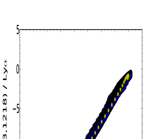
Figure 10: Log OV]/Ly$\alpha$ vs. log OVI+CIV/Ly$\alpha$. Every photoionization model of our grid is plotted (blue circles). Our ionization-bounded model sequence with $Z/Z_{\odot}$=1.1, $\alpha$=-1.0, and $n_{H}$=100 cm^-3 highlighted using yellow circles.

The luminosities of OVI $\lambda$1035 and CIV $\lambda$1549 similarly show a strong correlation with that of OV], but with a reversal near the high-ionization parameter end, leading to a larger dispersion and/or double-values, which reduces their individual usefulness as indicators of OV] luminosity. This degeneracy can be partially mitigated by summing the fluxes of OVI and CIV as illustrated in Fig.  10, where we show log OV] / Ly$\alpha$ vs log OVI+CIV / Ly$\alpha$. Using the same model sequence as described above, we obtain the relation:

OV] $\sim$ 0.07 $\times$ OVI+CIV

As a caveat, we emphasize that our corrections for OV] contamination are approximate and depend, among other parameters, on the gas chemical abundances and/or on the ionization parameter U. This is highlighted by Fig.  12, where we show OV]/NV vs. $Z/Z_{\odot}$ for model loci with three different values of U. We stress that observations of the OV] doublet will be essential to derive more accurate relations between the flux of this and other emission lines.

5 Discussion

5.1 General remarks

In the previous sections we have shown that for a certain range of conditions (or model parameters), the OV] $\lambda\lambda$1213.8,1218.3 doublet should significantly contaminate the Ly$\alpha$ fluxes of low density AGN-photoionized nebulae, i.e., the NLR or the Ly$\alpha$ halo. This result is in qualitative agreement with Shields et al. (1995), who obtained a similar result in relation to high-density, broad line region clouds. However, in contrast to Shields et al. (1995) for the high density BLR of Type 1 quasars (i.e., log $n_{H}$$\ga$10⁶ cm^-3), here we find that HeII $\lambda$1215.1 does not significantly contaminate the Ly$\alpha$ flux at the lower gas densities of the NLR (i.e., log $n_{H}$$\la$10⁴ cm^-3).

5.2 OV] contamination in Type 2 quasars

Thus far we have only considered model flux ratios, but it is also important to examine whether the observed UV line ratios of active galaxies suggest any significant contamination of their Ly$\alpha$ flux measurements by OV] or HeII $\lambda$1215.1. For this purpose, we use line flux measurements for 95 SDSS BOSS Type 2 quasars at z$>$2 from Silva et al. (2019), originally selected as candidate Type II quasars by Alexandroff et al. (2013). This sample has the advantage of having spectra obtained under a relatively homogeneous instrumental configuration (see Alewxandroff et al. 2013), and with line parameters determined using a single analysis methodology (see Silva et al. 2019). Furthermore, the redshift range of this sample places the Ly$\alpha$ line within the optical observational window, unlike lower-redshift objects (i.e., z$\la$2), thereby allowing comparision between the flux of Ly$\alpha$ and those of other UV lines such as NV, CIV, HeII, etc.

To complement this data sample, we also include line flux measurements for 12 radio galaxies at z$>$2 from the Keck II sample of Cimatti et al. (1998), Vernet et al. (2001) and Humphrey et al. (2008), selecting only those galaxies for which Ly$\alpha$, NV and HeII $\lambda$1640 have been detected. Again, this data sample has the advantage of being relatively homogenously observed and analysed.

The modeling discussed herein applies equally to the extended, narrow line emitting gas of Type 1 quasars. However, the broad (FWHM$\ga$ 2000 km s^-1) Ly$\alpha$ emission from the BLR usually overwhelms any narrow Ly$\alpha$, NV, and CIV emission from the NLR or Ly$\alpha$ halo, severely complicating the measurement and analysis of this narrow emission unless it is very extended (e.g. Borisova et al. 2016). For this reason, we do not include Type 1 quasars in our sample of objects. In any case, as Type 1 and Type 2 quasars are thought to be similar objects merely viewed at different orientations (e.g. Antonucci 1993 and references therein), conclusions derived from our Type 2 sample ought also to be applicable to Type 1 quasars.

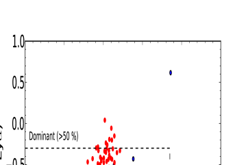
Figure 11: Plot of Log (2.5$\times$NV / Ly$\alpha$) vs. log (0.3$\times$HeII1640 / Ly$\alpha$) for z$\sim$2.5 radio galaxies from Vernet et al. (2001: blue circles), and Type 2 quasars at z$>$2 with detections of Ly$\alpha$, NV and HeII $\lambda$1640 from Silva et al. (2018: red circles). The vertical axis, log (2.5$\times$NV / Ly$\alpha$), is intended as a surrogate for log (OV] / Ly$\alpha$), while the horizontal axis, log (0.3$\times$HeII1640 / Ly$\alpha$), is a surrogate for log (HeII $\lambda$1215.1 / Ly$\alpha$).

The selected sample is shown in Fig.  11, where we plot log (2.5 $\times$ NV / Ly$\alpha$) vs. log (0.3 $\times$ HeII $\lambda$1640 / Ly$\alpha$) as estimators of the strength of OV] $\lambda\lambda$1213.8,1218.3 and HeII $\lambda$1215.1 relative to Ly$\alpha$, respectively (see §4.2).

The majority of the objects have 2.5 $\times$ NV / Ly$\alpha$ $\geq$ 0.1, implying that the OV] flux is usually significant compared to that of Ly$\alpha$ (90/107 or 84% of objects). In addition, we find that a small but significant fraction of the objects (10/107 or 9% of cases) have 2.5 $\times$ NV / Ly$\alpha$ $>$ 0.5, implying that the flux of OV] exceeds that of Ly$\alpha$.

Only in the case of one object shown in Fig.  11, the radio galaxy TXS 0211-122 (z=2.34), do we find a predicted value of 0.3$\times$HeII $\lambda$1640 / Ly$\alpha$ that lies above 0.5. In fact, its “Ly$\alpha$” flux can be more than accounted for by the combined expected fluxes of OV] and HeII $\lambda$1215.1, with (2.5 $\times$ NV / Ly$\alpha$) + (0.3$\times$HeII $\lambda$1640 / Ly$\alpha$) = 4.7. In this case it is clear that we have overestimated the flux of at least OV], if not also HeII $\lambda$1215.1, since our predicted OV]/Ly$\alpha$ ratio is 4.1. In other words, the predicted flux of OV], based on our extrapolation from NV, is 4.1 times higher than the observed flux of Ly$\alpha$ (see the Ly$\alpha$ and NV fluxes given in Vernet et al. 2001). We suggest that this overestimation might be the result of scattering and subsequent absorption of OV] and HeII photons by HI and dust, or an N/O abundance ratio that is several times higher than its Solar value (see e.g. van Ojik et al. 1994). It seems plausible that this ‘overestimation effect’ might also affect other objects in the sample, though it would be difficult to definitively verify without direct detections of OV].

As a further caveat, we stress that the selection criteria we have used to build our sample of quasars and radio galaxies specifically requires the detection of NV, and it is possible that this has introduced a bias favouring objects whose narrow line regions are highly-ionized and have a high abundance of nitrogen. Both of these conditions are expected to favour significant contamination of Ly$\alpha$ fluxes from OV] (see §3).

5.3 Prospects for direct detection of OV]

Despite the fact that photoionization models for AGN predict their presence (see also Ferland et al. 1992; Shields et al. 1995), HeII $\lambda$1215.1 or OV] $\lambda\lambda$1213.8,1218.3 have never, to the best of our knowledge, been directly detected in AGN-photoionized gas. Is there any prospect of directly detecting and deblending these lines from Ly$\alpha$ in active galaxies? We argue that under certain conditions, it should indeed be possible, at least in the case of OV]. If there is no velocity shift between OV] and Ly$\alpha$, then OV] $\lambda$1213.8 and OV] $\lambda$1218.3 would be offset with respect to Ly$\alpha$ by -1.9 Å  (-461 km s^-1) and +2.6 Å  (+649 km s^-1), respectively. This means that if Ly$\alpha$ is sufficiently narrow and is observed at sufficient spectral resolution and signal to noise ratio, then it should be possible to kinematically resolve OV] from Ly$\alpha$.

To illustrate this, we have created model spectra of the Ly$\alpha$ and NV spectral region as shown in Fig.  8. For the sake of simplicity, each line is represented by a single Gaussian emission profile, with all lines having the same full width at half maximum (FWHM) and, unless otherwise stated, we have not introduced any relative velocity shifts between lines. We have assumed the following flux ratios: OV] $\lambda$1213.8 / OV] $\lambda$1218.3 = 1.5 corresponding to the low density limit of this ratio (n_e $\leq$10⁴ cm^-3; McKenna et al. 1997); NV $\lambda$1238.8 / NV $\lambda$1242.8 = 2.0, corresponding to the optically thin case; OV] $\lambda\lambda$1213.8,1218.3 / NV $\lambda\lambda$1238.8,1242.8 = 2.5; OV] $\lambda\lambda$1213.8,1218.3 / Ly$\alpha$ = 0.2; HeII $\lambda$1215.1 / Ly$\alpha$ = 0.02. The continuum level has been set at 0.05 times the peak flux density of Ly$\alpha$. This value is consistent with observations of Type 2 active galaxies, although there can be large variation between objects (e.g., Vernet et al. 2001). In addition, we have added random (Gaussian) noise to our model spectra such that the $\sigma$ of the noise spectrum is 0.01 the peak flux density of the Ly$\alpha$ line. This value is somewhat arbitrary, given that the signal to noise ratio of the continuum depends on a variety of parameters, such as the UV continuum flux density of the target, the exposure time and conditions of the observations, the instrumental configuration, etc.

We have adopted FWHM values in the range 200 $<$ FWHM $<$ 1000 km s^-1, based on the observed kinematic properties of the NLR and extended emission halo of active galaxies, which are thought to be driven by a combination of gravitational motion and feedback activity (e.g., van Ojik et al. 1997; Baum & McCarthy 2000; Villar-Martín et al. 2003, 2007b; Das et al. 2005; Humphrey et al. 2006). In comparison, the extended Ly$\alpha$ emission associated with z$\ga$2 star forming galaxies typically lies in the range FWHM$\sim$100–500 km s^-1 (e.g. Leclercq et al. 2017).

We find that when the FWHM is large (e.g., $\geq$1000 km s^-1), OV] and Ly$\alpha$ are blended to such an extent that the velocity profile shows no discernable sign of the presence of the OV] lines (Fig.  8, top left). However, at FWHM$\sim$500-600 km s^-1 (Fig.  8, top right and centre left), the presence of OV] $\lambda$1218.3 becomes apparent as a small excess of flux in the red wing of the Ly$\alpha$ profile. At even lower values of FWHM (i.e., FWHM $\la$400 km s^-1: Fig.  8, centre right and bottom panels), OV] $\lambda$1218.3 is now resolved from Ly$\alpha$, rendering it detectable. The short wavelength component of the OV] doublet (OV] $\lambda$1213.8) becomes discernable at FWHM$\sim$300 km s^-1 (Fig.  8, bottom left), and is fully resolved from Ly$\alpha$ at FWHM$\la$200 km s^-1 (Fig.  8, bottom right), at which point it too should be readily detectable.

In Fig.  9 we show the impact of introducing a velocity shift between the high-ionization lines and Ly$\alpha$. We use a line FWHM of 500 km s^-1, and apply a velocity shift of -300,-200, -100, +100, +200 or +300 to the high-ionization lines, relative to the line of sight velocity of Ly$\alpha$. From the selection of model spectra shown in this Figure, it can be seen that even a small velocity shift (i.e., $\sim$100 km s^-1) between OV] and Ly$\alpha$ can alter the detectability of OV], and significantly change the total velocity profile of the blend. Generally speaking, a larger velocity shift improves the visibility of OV]. In the case where the OV] emission has a relative blueshift, we find the the flux asymmetry of the blend moves from its red wing to its blue wing. In the case of HeII $\lambda$1215.1, its -0.6 Å  offset from Ly$\alpha$ (equivalent to -141 km s^-1) and low expected relative flux should make this line highly challenging to directly detect (see Fig.  8).

If neglected, the presence of the OV doublet may complicate kinematic analyses that rely on the Ly$\alpha$ line. For instance, Fig.  8 reveals that when FWHM is in the range $\sim$400-600 km s^-1, the presence of strong OV] emission mimics the presence of a broader underlying kinematic component of Ly$\alpha$ emission, qualitatively similar to what is sometimes seen in high-z radio galaxies (e.g. Villar-Martín et al. 2003), potentially leading to the false detection of a gas outflow if a similar kinematic pattern cannot be confirmed in other emission lines (e.g., CIV, HeII $\lambda$1640, etc.). In addition, when one of the OV] lines is resolved from Ly$\alpha$, the dip in flux between the two lines could potentally be misinterpreted as a Ly$\alpha$ absorption feature, instead of as two resolved emission lines.

Thus, there is clearly some potential for ambiguity in the interpretation of the kinematic properties of the Ly$\alpha$+OV] blend, where a high velocity component of Ly$\alpha$ may be misinterpreted as OV] emission, and vice-versa. To overcome this degeneracy, we suggest extrapolating the expected wavelengths of the OV] lines from observations of other high-ionization lines, such as NV or CIV, to determine whether an observed feature in the profile of Ly$\alpha$ is likely to be an OV] line.

5.4 OV] as a diagnostic for AGN in Ly$\alpha$-emitters

We suggest that OV] $\lambda\lambda$1213.8,1218.3 should be useful as a means to confirm the presence of AGN activity in Ly$\alpha$-emitters at high redshift, if OV] is at least partly resolved from Ly$\alpha$ (e.g., at FWHM $\la$500 km s^-1; see Fig.  8). This is because ionizing O⁺³ to O⁺⁴, the species responsible for OV emission, requires a photon energy of $hv$$\geq$77.4 eV, which in turn requires an ionizing spectrum that is much harder than produced by young stellar populations, but which can be produced by an AGN. Thus, like NV $\lambda\lambda$1238,1242 (e.g. Villar-Martín et al. 1999), a detection of OV] emission ought to be considered a ‘smoking gun’ of AGN activity in a Ly$\alpha$-emitter.

A further point of interest is that under some circumstances, OV] should be easier to detect than NV. For instance, given the secondary enrichment of the N abundance, the OV]/NV flux ratio is expected to increase significantly towards lower gas metallicity as shown in Fig.  12, such that OV] should become more easily detectable than NV for sub-Solar gas metallicities, provided OV] and Ly$\alpha$ can be deblended. The precise range of parameters where OV] should become easier to detect than NV is model dependent, but based on our modelling we expect this to be the case when FWHM $\la$500 km s^-1 and 0.1$\la$$Z/Z_{\odot}$$\la$1.0 – properties broadly corresponding to those expected for low to intermediate mass Ly$\alpha$-emitters at high redshift (e.g. McGreer et al. 2018; Sobral et al. 2018a,b; Mainali et al. 2018; Leclercq et al. 2017; Jiang et al. 2013; Fosbury et al. 2003).

Thus, as advances in instrumentation and telescope collecting area provide access to ever more distant and ever fainter galaxies (e.g. Hashimoto et al. 2017; Ouchi et al. 2018), we expect OV] to become a useful diagnostic of the presence of AGN activity in high-z Ly$\alpha$-emitting systems, particularly in intermediate to low mass galaxies whose gas metallicity is sub-Solar.

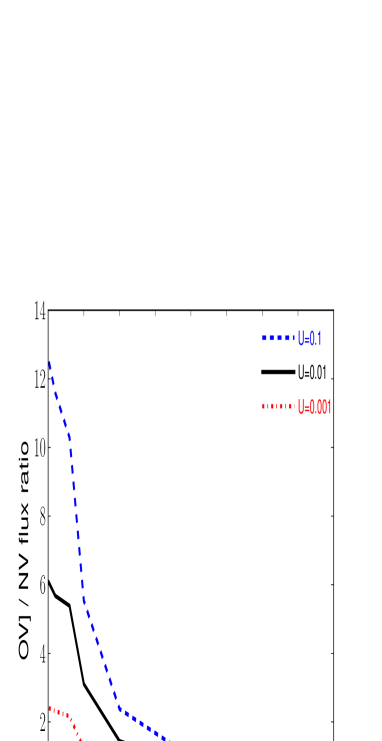
Figure 12: OV] over NV versus gas metallicity $Z/Z_{\odot}$ for $\alpha$=-1.0 and $n_{H}$ = 100 cm^-3, for three different values of ionization parameter U. The shown models are ionization-bounded (optically-thick). As discussed in the main text, the OV]/NV ratio increases with decreasing gas metallicity $Z/Z_{\odot}$, such that OV] may become more easily detectable than NV when 0.1$\la Z/Z_{\odot}\la$1.0, provided OV] and Ly$\alpha$ can be deblended.

6 Summary

We have used a grid of photoionization models to examine the potential impact of OV] $\lambda\lambda$1213.8,1218.3 and HeII $\lambda$1215.1 emission on measurements of the Ly$\alpha$ flux from the NLR and Ly$\alpha$ halos of active galaxies. We find that the HeII flux is essentially always negligible, but OV] can contribute significantly ($\ga$10%) when the ionization parameter and the gas metallicity are high (log U $\ga$-2; $Z/Z_{\odot}$$\ga$0.3). We also find that using optically-thin clouds can increase the relative contributions from OV] and HeII.

In addition, we have provided means to estimate the fluxes of HeII $\lambda$1215.1 and OV] $\lambda\lambda$1213.8,1218.3 by extrapolating from other UV emission lines, and have estimated the contribution from these lines in a sample of 107 Type 2 active galaxies (QSO2s and HzRGs) at z$>$2, finding evidence for significant contamination of Ly$\alpha$ fluxes ($\geq 10\%$) in 84% of cases. This suggests that Ly$\alpha$ flux measurements of type 2 active galaxies are often contaminated at the $\ga$10% level by these other lines.

We have also found that the presence of OV] emission can impact the apparent kinematics of Ly$\alpha$, potentially mimicking the presence of high-velocity outflows.

Additionally, we have shown that, where its flux is significant, OV] ought to be detectable when the FWHM of Ly$\alpha$ is less than $\sim$500 km s^-1, and we have proposed using detection of OV] as a new diagnostic of AGN activity in high-z Ly$\alpha$ emitters.

References

- Alexandroff et al. (2013) Alexandroff R., et al., 2013, MNRAS, 435, 3306
- Antonucci (1993) Antonucci R., 1993, ARA&A, 31, 473
- Arrigoni Battaia et al. (2018) Arrigoni Battaia F., Hennawi J. F., Prochaska J. X., Oñorbe J., Farina E. P., Cantalupo S., Lusso E., 2018, arXiv, arXiv:1808.10857
- Asplund, Grevesse, & Jacques Sauval (2006) Asplund M., Grevesse N., Jacques Sauval A., 2006, NuPhA, 777, 1
- Baum & McCarthy (2000) Baum S. A., McCarthy P. J., 2000, AJ, 119, 2634
- Binette, Dopita, & Tuohy (1985) Binette L., Dopita M. A., Tuohy I. R., 1985, ApJ, 297, 476
- Binette et al. (2012) Binette L., Matadamas R., Hägele G. F., Nicholls D. C., Magris C. G., Peña-Guerrero M. Á., Morisset C., Rodríguez-González A., 2012, A&A, 547, A29
- Borisova et al. (2016) Borisova E., et al., 2016, ApJ, 831, 39
- Christensen et al. (2006) Christensen L., Jahnke K., Wisotzki L., Sánchez S. F., 2006, A&A, 459, 717
- Cimatti et al. (1998) Cimatti A., di Serego Alighieri S., Vernet J., Cohen M. H., Fosbury R. A. E., 1998, ApJ, 499, L21
- Das et al. (2005) Das V., et al., 2005, AJ, 130, 945
- Dijkstra, Haiman, & Spaans (2006) Dijkstra M., Haiman Z., Spaans M., 2006, ApJ, 649, 14
- Dors et al. (2018) Dors O. L., Agarwal B., Hägele G. F., Cardaci M. V., Rydberg C.-E., Riffel R. A., Oliveira A. S., Krabbe A. C., 2018, MNRAS, 479, 2294
- Ferland et al. (1992) Ferland G. J., Peterson B. M., Horne K., Welsh W. F., Nahar S. N., 1992, ApJ, 387, 95
- Ferruit et al. (1997) Ferruit P., Binette L., Sutherland R. S., Pecontal E., 1997, A&A, 322, 73
- Fosbury et al. (2003) Fosbury R. A. E., et al., 2003, ApJ, 596, 797
- Hashimoto et al. (2017) Hashimoto T., et al., 2017, A&A, 608, A10
- Heckman et al. (1991) Heckman T. M., Lehnert M. D., Miley G. K., van Breugel W., 1991, ApJ, 381, 373
- Henry, Edmunds, & Köppen (2000) Henry R. B. C., Edmunds M. G., Köppen J., 2000, ApJ, 541, 660
- Humphrey et al. (2006) Humphrey A., Villar-Martín M., Fosbury R., Vernet J., di Serego Alighieri S., 2006, MNRAS, 369, 1103
- Humphrey et al. (2008) Humphrey A., Villar-Martín M., Vernet J., Fosbury R., di Serego Alighieri S., Binette L., 2008, MNRAS, 383, 11
- Humphrey et al. (2018) Humphrey A., Villar-Martín M., Binette L., Raj R., 2018, arXiv, arXiv:1810.04463
- Jiang et al. (2013) Jiang L., et al., 2013, ApJ, 773, 153
- Leclercq et al. (2017) Leclercq F., et al., 2017, A&A, 608, A8
- Mainali et al. (2018) Mainali R., et al., 2018, MNRAS, 479, 1180
- McGreer et al. (2018) McGreer I. D., et al., 2018, MNRAS, 479, 435
- McKenna et al. (1997) McKenna F. C., Keenan F. P., Aller L. H., Hyung S., Feibelman W. A., Berrington K. A., Fleming J., Hibbert A., 1997, ApJ, 486, 571 Osterbrock D.E., Ferland G., 2005, Astrophysics of Gaseous Nebulae and Active Galactic Nuclei, Second Edition, University Science Books
- Ouchi et al. (2018) Ouchi M., et al., 2018, PASJ, 70, S13
- Pogge (1988) Pogge R. W., 1988, ApJ, 328, 519
- Reuland et al. (2003) Reuland M., et al., 2003, ApJ, 592, 755
- Shields, Ferland, & Peterson (1995) Shields J. C., Ferland G. J., Peterson B. M., 1995, ApJ, 441, 507
- Silva et al. (2018) Silva M., et al., 2018a, MNRAS, 474, 3649
- Silva et al. (2018) Silva M., et al., 2018b, in prep
- Sobral et al. (2018) Sobral D., et al., 2018, MNRAS, 477, 2817
- Sobral et al. (2018) Sobral D., Santos S., Matthee J., Paulino-Afonso A., Ribeiro B., Calhau J., Khostovan A. A., 2018, MNRAS, 476, 4725
- van Ojik et al. (1994) van Ojik R., Rottgering H. J. A., Miley G. K., Bremer M. N., Macchetto F., Chambers K. C., 1994, A&A, 289, 54
- van Ojik et al. (1997) van Ojik R., Roettgering H. J. A., Miley G. K., Hunstead R. W., 1997, A&A, 317, 358
- Vernet et al. (2001) Vernet J., Fosbury R. A. E., Villar-Martín M., Cohen M. H., Cimatti A., di Serego Alighieri S., Goodrich R. W., 2001, A&A, 366, 7
- Vernet et al. (2017) Vernet J., et al., 2017, A&A, 602, L6
- Villar-Martin, Binette, & Fosbury (1996) Villar-Martin M., Binette L., Fosbury R. A. E., 1996, A&A, 312, 751
- Villar-Martín et al. (2002) Villar-Martín M., Vernet J., di Serego Alighieri S., Fosbury R., Pentericci L., Cohen M., Goodrich R., Humphrey A., 2002, MNRAS, 336, 436
- Villar-Martín et al. (2003) Villar-Martín M., Vernet J., di Serego Alighieri S., Fosbury R., Humphrey A., Pentericci L., 2003, MNRAS, 346, 273
- Villar-Martín et al. (2007) Villar-Martín M., Humphrey A., De Breuck C., Fosbury R., Binette L., Vernet J., 2007a, MNRAS, 375, 1299
- Villar-Martín et al. (2007) Villar-Martín M., Sánchez S. F., Humphrey A., Dijkstra M., di Serego Alighieri S., De Breuck C., González Delgado R., 2007b, MNRAS, 378, 416
- Weidinger, Møller, & Fynbo (2004) Weidinger M., Møller P., Fynbo J. P. U., 2004, Natur, 430, 999
- Wilman et al. (2004) Wilman R. J., Jarvis M. J., Röttgering H. J. A., Binette L., 2004, MNRAS, 351, 1109
- Wilman et al. (2005) Wilman R. J., Gerssen J., Bower R. G., Morris S. L., Bacon R., de Zeeuw P. T., Davies R. L., 2005, Natur, 436, 227