Abstract

We develop a new Low-level, First-order Probabilistic Programming Language (LF-PPL) suited for models containing a mix of continuous, discrete, and/or piecewise-continuous variables. The key success of this language and its compilation scheme is in its ability to automatically distinguish parameters the density function is discontinuous with respect to, while further providing runtime checks for boundary crossings. This enables the introduction of new inference engines that are able to exploit gradient information, while remaining efficient for models which are not everywhere differentiable. We demonstrate this ability by incorporating a discontinuous Hamiltonian Monte Carlo (DHMC) inference engine that is able to deliver automated and efficient inference for non-differentiable models. Our system is backed up by a mathematical formalism that ensures that any model expressed in this language has a density with measure zero discontinuities to maintain the validity of the inference engine.

1 Introduction

Non-differentiable densities arise in a huge variety of common probabilistic models [1, 2]. Often, but not exclusively, they occur due to the presence of discrete variables. In the context of probabilistic programming [3, 4, 5, 6] such densities are often induced via branching, i.e. if-else statements, where the predicates depend upon the latent variables of the model. Unfortunately, performing efficient and scalable inference in models with non-differentiable densities is difficult and algorithms adapted for such problems typically require specific knowledge about the discontinuities [7, 8, 9], such as which variables the target density is discontinuous with respect to and catching occurrences of the sampler crossing a discontinuity boundary. However, detecting when discontinuities occur is difficult and problem dependent. Consequently, automating specialized inference algorithms in probabilistic programming languages (PPLs) is challenging.

To address this problem, we introduce a new Low-level First-order Probabilistic Programming Language (LF-PPL), with a novel accompanying compilation scheme. Our language is based around carefully chosen mathematical constraints, such that the set of discontinuities in the density function of any model written in LF-PPL will have measure zero. This is an essential property for many inference algorithms designed for non-differentiable densities [7, 8, 9, 10, 11]. Our accompanying compilation scheme automatically classifies discontinuous and continuous random variables for any model specified in our language. Moreover, this scheme can be used to detect transitions across discontinuity boundaries at runtime, providing important information for running such inference schemes.

Relative to previous languages, LF-PPL enables one to incorporate a broader class of specialized inference techniques as automated inference engines. In doing so, it removes the burden from the user of manually establishing which variables the target is not differentiable with respect to. Its low-level nature is driven by a desire to establish the minimum language requirements to support inference engines tailored to problems with measure-zero discontinuities, and to allow for a formal proof of correctness. Though still usable in its own right, our main intention is that it will be used as a compilation target for existing systems, or as an intermediate system for designing new languages.

There are a number of different derivative-based inference paradigms for which LF-PPL can help extend to non-differentiable setups [7, 8, 9, 10, 11]. Of particular note, are stochastic variational inference (SVI) [12, 13, 14, 15] and Hamiltonian Monte Carlo (HMC) [16, 17], two of the most widely used approaches for probabilistic programming inference.

In the context of the former, [9] recently showed that the reparameterization trick can be generalized to piecewise differentiable models when the non-differentiable boundaries can be identified, leading to an approach which provides significant improvements over previous methods that do not explicitly account for the discontinuities. LF-PPL provides a framework that could be used to apply their approach in a probabilistic programming setting, thereby paving the way for significant performance improvements for such models.

Similarly, many variants of HMC have been proposed in recent years to improve the sample efficiency and scalability when the target density is non-differentiable [7, 8, 18, 19, 20]. Despite this, no probabilitic programming systems (PPSs) support these tailored approaches at present, as the underlying languages are not able to extract the necessary information for their automation. The novel compilation approach of LF-PPL provides key information for running such approaches, enabling their implementation as automated inference engines. We realize this potential by implementing Discontinuous HMC (DHMC) [8] as an inference engine in LF-PPL, allowing for efficient, automated, HMC-based inference in models with a mixture of continuous and discontinuous variables.

2 Background and Related Work

There exists a number of different approaches to probabilistic programming that are built around a variety of semantics and inference engines. Of particular relevance to our work are PPSs designed around derivative based inference methods that exploit automatic differentiation [21], such as Stan [6], PyMC3 [22], Edward [23], Turing [24] and Pyro [25]. Derivative based inference algorithms have been an essential component in enabling these systems to provide efficient and, in particular, scalable inference, permitting both large datasets and high dimensional models.

One important challenge for these systems occurs in dealing with probabilistic programs that contain discontinuous densities and/or variables. From the statistical perspective, dealing with discontinuities is often important for conducting effective inference. For example, in HMC, discontinuities can cause statistical inefficiency by inducing large errors in the leapfrog integrator, leading to potentially very low acceptance rates [7, 8]. In other words, though the leapfrog integrator remains a valid, reversible, MCMC proposal even when discontinuities break the reversibility of the Hamiltonian dynamics themselves, they can undermine the effectiveness of this proposal.

Different methods have been suggested to improve inference performance in models with discontinuous densities. For example, they use sophisticated integrators in the HMC setting to remain effective when there are discontinuities. Analogously, in the variational inference and deep learning literature, reparameterization methods have been proposed that allow training for discontinuous targets and discrete variables [9, 26].

However, these advanced methods are, in general, not incorporated in existing gradient-based PPSs, as existing systems do not have adequate support to deal with the discontinuities in the density functions of the model defined by probabilistic programs. This is usually necessary to guarantee the correct execution of those inference methods in an automated fashion, as many require the set of discontinuities to be of measure zero. That is, the union of all points where the density is discontinuous have zero measure with respect to the Lebesgue measure. In addition to this, some further methods require knowledge of where the discontinuities are, or at least catching occurrences of discontinuity boundaries being crossed.

Of particular relevance to our language and compilation scheme are compilers which compile the program to an artifact representing a direct acyclic graphical model (DAG), such as those employed in BUGS [27] and, in particular, the first order PPL (FOPPL) explored in [28]. Although the dependency structures of the programs in our language are established in a similar manner, unlike these setups, programs in our language will not always correspond to a DAG, due to different restrictions on our density factors, as will be explained in the next section. We also impose necessary constraints on the language by limiting the functions allowed to ensure that the advanced inference processes remain valid.

3 The Language

LF-PPL adopts a Lisp-like syntax, like that of Church [4] and Anglican [5]. The syntax contains two key special forms, sample and observe, between which the distribution of the query is defined and whose interpretation and syntax is analogous to that of Anglican.

More precisely, sample is used for drawing random variables, returning that variable, and observe factors the density of the program using existing variables and fixed observations, returning zero. Both special forms are designed to take a distribution object as input, with observe further taking an observed value. These distribution objects form the elementary random procedures of the language and are constructed using one of a number of internal constructors for common objects such as normal and bernoulli. Figure 1 shows an example of an LF-PPL program.

A distribution object constructor of particular note is factor, which can only be used with observe. Including the statement (observe (factor log-p) _) will factor the program density using the value of (exp log-p), with no dependency on the observed value itself (here _). The significance of factor is that it allows the specification of arbitrary unnormalized target distributions, quantified as log-p which can be generated internally in the program, and thus have the form of any deterministic function of the variables that can be written in the language.

⬇

(let [x (sample (uniform 0 1))]

(if (< (- q x) 0)

(observe (normal 1 1) y)

(observe (normal 0 1) y))

(< (- q x) 0))

Figure 1: An example LF-PPL program sampling $x$ from a uniform random variable and invoking a choice between two observe statements that factor the trace weight using different Gaussian likelihoods. The (< (- q x) 0) term, which is usually written as ${((q-x)<0)}$, represents a Bernoulli variable parameterized by q and its boolean value also corresponds to which branch of the if statement is taken. The slightly unusual writing of the program is due to its deliberate low-level nature, with almost all syntactic sugar removed. One sugar that has been left in for exposition is an additional term in the let block, i.e. (let [x e] e e), which can be trivially unraveled.

Unlike many first-order PPLs, such as that of [28], LF-PPL programs do not permit interpretation as DAGs because we allow the observation of internally sampled variables and the use of factor. This increases the range of models that can be encoded and is, for example, critical in allowing undirected models to be written. LF-PPL programs need not correspond to a correctly normalized joint formed by the combination of prior and likelihood terms. Instead we interpret the density of a program in the manner outlined by [29, §4.3.2 and §4.4.3], noting that for any LF-PPL program, the number of sample and observe statements (i.e. $n_{x}$ and $n_{y}$ in their notation) must be fixed, a restriction that is checked during the compilation.

To formalize the syntax of LF-PPL, let us use $x$ for a real-valued variable, $c$ for a real number, op for an analytic primitive operation on reals, such as +, -, *, / and exp, and $d$ for a distribution object whose density is defined with respect to a Lebesgue measure and is piecewise smooth under analytic partition (See Definition 1). Then the syntax of expressions $e$ in our language are given as:

$${{{{{\begin{array}[]{@{}r@{}c@{}l@{}}e&\,::=&x\mid c\mid(\text{\leavevmode\lstinline{{\lst@@@set@language\lst@@@set@numbers\lst@@@set@frame\lst@@@set@rulecolor\lst@@@set@language\lst@@@set@language{\@listingGroup{ltx_lst_keywords7}{\color[rgb]{0.0,0.6,0.5}op}}}}}}\ e\,\ldots\,e)\mid(\text{\leavevmode\lstinline{{\lst@@@set@language\lst@@@set@numbers\lst@@@set@frame\lst@@@set@rulecolor\lst@@@set@language\lst@@@set@language{\@listingGroup{ltx_lst_keywords3}{\color[rgb]{0.60,0.0,0.0}if}}}}}}\ (<e\ 0)\ e\ e)\mid(\text{\leavevmode\lstinline{{\lst@@@set@language\lst@@@set@numbers\lst@@@set@frame\lst@@@set@rulecolor\lst@@@set@language\lst@@@set@language{\@listingGroup{ltx_lst_keywords3}{\color[rgb]{0.60,0.0,0.0}let}}}}}}\ [x\ e]\ e)\\ &\,\,\,\,\,\,\mid&(\text{\leavevmode\lstinline{{\lst@@@set@language\lst@@@set@numbers\lst@@@set@frame\lst@@@set@rulecolor\lst@@@set@language\lst@@@set@language{\@listingGroup{ltx_lst_keywords8}{\color[rgb]{0,0.3,0.7}sample}}}}}}\ (d\ e\,\ldots\,e))\mid(\text{\leavevmode\lstinline{{\lst@@@set@language\lst@@@set@numbers\lst@@@set@frame\lst@@@set@rulecolor\lst@@@set@language\lst@@@set@language{\@listingGroup{ltx_lst_keywords8}{\color[rgb]{0,0.3,0.7}observe}}}}}}\ (d\ e\,\ldots\,e)\ c)\vspace{-5pt}\par\end{array}$$

Our syntax is deliberately low-level to permit theoretical analysis and aid the exposition of the compiler. However, common syntactic sugar such as for-loops and higher-level branching statements can be trivially included using straightforward unravellings. Similarly, we can permit discrete variable distribution objects by noting that these can themselves be desugared to a combination of continuous random variables and branching statements. Thus, it is straightforward to extend this minimalistic framework to a more user-friendly language using standard compilation approaches, such that LF-PPL will form an intermediate representation. For implementation and code, see https://github.com/bradleygramhansen/PyLFPPL.

4 Compilation Scheme

We now provide a high-level description of how the compilation process works. Specifically, we will show how it transforms an arbitrary LF-PPL program to a representation that can be exploited by an inference engine that makes of use of discontinuity information.

The compilation scheme performs three core tasks: a) finding the variables which the target is discontinuous with respect to, b) extracting the density of the program to a convenient form that can be used by an inference engine, and c) allowing boundary crossings to be detected at runtime. Key to providing these features is the construction of an internal representation of the program that specifies the dependency structure of the variables, the Linearized Intermediate Representation (LIR). The LIR contains vertices, arc pairs, and information of the if predicates. Each vertex of the LIR denotes a sample or observe statement, of which only a finite and fix number can occur in LF-PPL. The arcs of the LIR define both the probabilistic and if condition dependencies of the variables. The former of these are constructed in same was as is done in the FOPPL compiler detailed in [28].

Using the dependency structure represented by the LIR, we can establish which variables are capable of changing the path taken by a program trace, that is the change the branch taken by one or more if statements. Because discontinuities only occur in LF-PPL through if statements, the target must be continuous with respect to any variables not capable of changing the traversed path. We can thus mark these variables as being “continuous”. Though it is possible for the target to still be continuous with respect to variables that appear in, or have dependent variables appearing in, the branching function of an if statement, such cases cannot, in general, be statically established. We therefore mark all such variables as “discontinuous”.

To extract the density to a convenient form for the inference engine, the compiler transforms the program into a collection four sets—$\Delta,\Gamma,D,$ and $F$—by recursively applying the translation rules given in Section 5.2. Here $\Delta$ specifies the set of all variables sampled in the program, while $\Gamma$ specifies only the variables marked as discontinuous. $D$ represents the density associated with all the sample statements in a program, while $F$ represents the density factors originating for the observe statements, along with information on the program return value. These densities are themselves represented through a collection of smooth density terms and indicator functions truncating them into disjoint regions, each corresponding to a particular program path. This construction will be discussed in depth in Section 5.2.

To catch boundary crossings at run time, each if predicate is assigned a unique boolean variable within the LIR. We refer to these variables as branching variables. The boolean value of the branching variable denotes whether the current sample falls into the true or false branch of the corresponding if statement and is used to signal boundary crossings at runtime. Specifically, if one branching variable changes its boolean value, this indicates that at least one sampled variables effecting that if predicate has crossed the boundary. The inference engine can therefore track changes in the set of all Boolean values to catch the boundary crossings.

We finish the section by noting two limitations of the compiler and for discontinuity detection more generally. Firstly, we note that it is possible to construct programs which have piecewise smooth densities that contain regions of zero density. Though it is important to allow this ability, for example to construct truncated distributions, it may cause issues for certain inference algorithms if it causes the target to have disconnected regions of non-zero density. As analytic densities are either zero everywhere or “almost-nowhere” (see Section 5.1), we (informally) have that all realizations of a program that take a particular path will either have zero density or all have a non-zero density. Consequently, it is relatively straight forward to establish if a program has regions of zero density. However, whether these regions lead to “gaps” is far more challenging, and potentially impossible, to establish. Moreover, constructing inference procedures for such problems is extremely challenging. We therefore do not attempt to tackle this issue in the current work.

A second limitation is that changes in the vector of branching variables is only a sufficient condition for the occurrence of a boundary crossing. This is because it is possible for multiple boundaries to be crossed in a single update that results in the new sample following the same path as the old one. For example, when moving from $x=-0.5$ to $x=1.5$ then a branching variable corresponding to $x^{3}-x>0$ returns true in both cases even though we have crossed two boundaries. The problem of establishing with certainty that no boundaries have been crossed when moving between two points is mathematically intractable in the general case. As this problem is not specific to the probabilistic programming setting, we do not give it further consideration here, noting only that it is important from the perspective of designing inference algorithms that convergence is not undermined by such occurrences.

5 Mathematical Foundation and Compilation Details

Our story so far was developed by introducing a low-level first-order probabilistic programming language (LF-PPL) and its accompanying compilation scheme. We shall now expose the underlying mathematical details, which ensure that discontinuities contained within the densities of the programs one can compile in LF-PPL are of a suitable measure. This enables us to satisfy the requirements of several inference algorithms for non-differentiable densities. We also provide the formal translation rules of the LF-PPL, which are built around these mathematical underpinnings.

5.1 Piecewise Smooth Functions

A function $\mathcal{G}:\mathbb{R}^{k}\to\mathbb{R}$ is analytic if it is infinitely differentiable and its multivariate Taylor expansion at any point $x_{0}\in\mathbb{R}^{k}$ absolutely converges to $\mathcal{G}$ point-wise in a neighborhood of $x_{0}$. Most primitive functions that we encounter in machine learning and statistics are analytic, and the composition of analytic functions is also analytic.

Definition 1.

A function $\mathcal{G}:\mathbb{R}^{k}\to\mathbb{R}$ is piecewise smooth under analytic partition if it has the following form:

$$\mathcal{G}(x)=\sum_{i=1}^{N}\left(\prod_{j=1}^{M_{i}}\mathbbm{1}[p_{i,j}(x)\geq 0]\cdot\prod_{l=1}^{O_{i}}\mathbbm{1}[q_{i,l}(x)<0]\cdot h_{i}(x)\right)$$

where

1. the $p_{i,j},q_{i,l}:\mathbb{R}^{k}\to\mathbb{R}$ are analytic;

2. the $h_{i}:\mathbb{R}^{k}\to\mathbb{R}$ are smooth;

3. $N$ is a positive integer or $\infty$;

4. $M_{i},O_{i}$ are non-negative integers; and

5. the indicator functions

   $$\prod_{j=1}^{M_{i}}\mathbbm{1}[p_{i,j}(x)\geq 0]\cdot\prod_{l=1}^{O_{i}}\mathbbm{1}[q_{i,l}(x)<0]\vspace{-5pt}$$

   for the indices $i$ define a partition of $\mathbb{R}^{k}$, that is, the following family forms a partition of $\mathbb{R}^{k}$:

   $$\bigg{\{}\left\{x\,{\in}\,\mathbb{R}^{k}\;\Big{|}\;\begin{array}[]{@{}l@{}}\forall j\,p_{i,j}(x)\,{\geq}\,0,\,\forall l\,q_{i,l}(x)\,{<}\,0\end{array}\right\}\Big{|}\,1\,{\leq}\,i\,{\leq}\,N\bigg{\}}.$$

Intuitively, $\mathcal{G}$ is a function defined by partitioning $\mathbb{R}^{k}$ into finitely or countably many regions and using a smooth function $h_{i}$ within region $i$. The products of the indicator functions of these summands form a partition of $\mathbb{R}^{k}$, so that only one of these products gets evaluated to a non-zero value at $x$. To evaluate the sum, we just need to evaluate these products at $x$ one-by-one until we find one that returns a non-zero value. Then, we have to compute the function $h_{i}$ corresponding to this product at the input $x$. Even though the number of summands (regions) $N$ in the definition is countably infinite, we can still compute the sum at a given $x$.

Theorem 1.

If an unnormalized density $\mathcal{P}:\mathbb{R}^{n}\to\mathbb{R}_{+}$ has the form of Definition 1 and so is piecewise smooth under analytic partition, then there exists a (Borel) measurable subset $A\subseteq\mathbb{R}^{n}$ such that $\mathcal{P}$ is differentiable outside of $A$ and the Lebesgue measure of $A$ is zero.

The proof is given in Appendix A. The target density being almost everywhere differentiable with discontinuities of measure zero is an important property required by many inference techniques for non-differentiable models [8]. As we shall prove in Section 5.2, any program that can be compiled in LF-PPL constructs a density in the form of Definition 1, and thus satisfies this necessary condition.

5.2 Translation Rules

5.2.1 Overview

The compilation scheme $e\leadsto(\Delta,\Gamma,D,F)$ translates a program, which can be denoted as an expression $e$ according to the syntax in Section 3, to a quadruple of sets $(\Delta,\Gamma,D,F)$. The first set $\Delta$ represents the set of all sampled random variables. All variables generated from sample statements in $e$ will be recognized and stored in $\Delta$. Variables that have not occurred in any if predicate are guaranteed to be continuous. Otherwise, they will be also put in $\Gamma\subseteq\Delta$, as the overall density is discontinuous with respect to them. $D$ represents the densities from sample statements and has the form of a set of the pairs, i.e. $D=\{(\eta_{1},k_{1}),\dots,(\eta_{N_{D}},k_{N_{D}})\}$, where $N_{D}$ is the number of the pairs, $\eta$ denotes a product of indicator functions indicating the partition of the space, and $k$ represents the products of the densities defined by the sample statements. The last set $F$ contains the densities from observe statements and the return expression of $e$. It is a set of tuples $F=\{(\zeta_{1},l_{1},v_{1}),\dots,(\zeta_{N_{F}},l_{N_{F}},v_{N_{F}})\}$, where $N_{F}$ is the number of the tuples, $\zeta$ functions similar to $\eta$, $l$ is the product of the densities defined by observe statements and $v$ denotes the returning expression. Note that it is a design choice to have $v$ included in $F$.

Given $e\leadsto(\Delta,\Gamma,D,F)$, one can then construct the unnormalized density defined by the program $e$ as

$$\mathcal{P}\,{:=}\Big{(}\sum_{i=1}^{N_{D}}\eta_{i}{\cdot}k_{i}\Big{)}\cdot\Big{(}\sum_{j=1}^{N_{F}}\zeta_{j}{\cdot}l_{j}\Big{)}$$ (1)

which by Theorem 2 will be piecewise smooth under analytic partitions.

Recall that by assumption, the density of each distribution type $d$ is piecewise smooth under analytic partition when viewed as a function of a sampled value and its parameters. Thus, we can assume that the probability density of a distribution has the form in Definition 1. For each distribution $d$, we define a set of pairs $\Phi^{(d)}{=}\{(\psi_{1},\phi_{1}),\dots,(\psi_{N_{\Phi}},\phi_{N_{\Phi}})\}$ where $N_{\Phi}$ is the number of the partitions, $\psi$ denotes the product of indicator functions indicating the partition of the space, taking the form of $\prod_{j=1}^{M_{i}}\mathbbm{1}[p_{i,j}(\mathbf{x}){\geq}0]\cdot\prod_{l=1}^{O_{i}}\mathbbm{1}[q_{i,l}(\mathbf{x}){<}0]$, and $\phi$ represents a smooth probability density function within that partition. One can then construct the probability density function $\mathcal{P}_{d}$ for $d$ from $\Phi^{(d)}$. For given parameters $x_{1},\ldots,x_{s}$ of the distribution $d$ and a given sample value $x_{0}$, we let $\mathbf{x}=(x_{0},\ldots,x_{s})$ and the probability density function defined by $d$ is,

$$\mathcal{P}_{d}(x_{0};x_{1},\ldots,x_{s})={\sum}_{n=1}^{N_{\Phi}}\psi_{n}(\mathbf{x})\cdot\phi_{n}(\mathbf{x})\vspace{-8pt}$$

For example, given $x_{0}$ drawn from normal distribution $\mathcal{N}(\mu,\sigma)$, we have $\Phi^{(d)}=\left\{\left(1,\mathcal{N}(x_{0}\,;\mu,\sigma)\right)\right\}$ and $\mathcal{P}_{d}(x_{0};\mu,\sigma)=\mathcal{N}(x_{0}\,;\mu,\sigma)$. Similarly a uniform $\mathcal{U}(a,b)$ sampled variable $x_{0}$ has $\Phi^{(d)}$ as

$$\big{\{} \left(\mathbbm{1}[x_{0}{-}a{<}0],\,0\right),\ \left(\mathbbm{1}[b{-}x_{0}{<}0],\,0\right),$$

$$\left(\mathbbm{1}[x_{0}{-}a{\geq}0]{\cdot}\mathbbm{1}[b{-}x_{0}{\geq}0],\,\mathcal{U}(x_{0};a,b)\right)\big{\}},\vspace{-10pt}$$

and $\mathcal{P}_{d}=\mathbbm{1}[x_{0}{-}a{\geq}0]{\cdot}\mathbbm{1}[b{-}x_{0}{\geq}0]\cdot\mathcal{U}(x_{0};a,b)$. Note that in practice one can omit the pair $(\psi_{n},\phi_{n})$ in $\Phi^{(d)}$ when $\phi_{n}{=}\,0$ for simplicity and the probability density in the region denoting by the corresponding $\psi_{n}$ is zero.

5.2.2 Formal Translation Rules

The translation process $e\leadsto(\Delta,\Gamma,D,F)$, is defined recursively on the structure of $e$. We present this recursive definition using the following notation

$$\mbox{conclusion}\mbox{premise}\vspace{-5pt}$$

which says that if the premise holds, then the conclusion holds too. Also, for real-valued functions $f(x_{1},\ldots,x_{n})$ and $f^{\prime}(x_{1},\ldots,x_{n})$ on real-valued inputs, we write $f[x_{i}:=f^{\prime}]$ to denote the composition $f(x_{1},\ldots,x_{i-1},f^{\prime}(x_{1},\ldots,x_{n}),x_{i+1},\ldots,x_{n}).$ We now define the formal translation rules.

The first two rules define how we map the set of variables $x$ and the set of constants $c$, to their unnormalized density and the values at which they are evaluated.

$$\begin{array}[]{@{}c@{}}x\leadsto(\{x\},\emptyset,\,\{(1,1)\},\,\{(1,1,x)\})\\[8.61108pt] c\leadsto(\emptyset,\emptyset,\,\{(1,1)\},\,\{(1,1,c)\})\end{array}$$

The third rule allows one to translate the primitive operations op defined in the LF-PPL, such as +, -, * and / with their argument expressions $e_{1}$ to $e_{n}$, where $e_{1}$ to $e_{n}$ will be evaluated first. Note that $(\eta_{i},k_{i})\in D_{i}$ represents the enumeration of all $(\eta_{i},k_{i})$ pairs in $D_{i}$ and the result of this operation among all the $D_{i}$ is the possible combination of all their elements. For example, given three sets $D_{1}$, $D_{2}$ and $D_{3}$ which have three, one and two pairs respectively as their elements, the result set $D^{\prime}$ will have six pairs. This notation holds to the rest of the paper.

$${{\begin{array}[]{@{}c@{}}(\text{\leavevmode\lstinline{{\lst@@@set@language\lst@@@set@numbers\lst@@@set@frame\lst@@@set@rulecolor\lst@@@set@language\lst@@@set@language{\@listingGroup{ltx_lst_keywords7}{\color[rgb]{0.0,0.6,0.5}op}}}}}}\ e_{1}\ \ldots\ e_{n})\leadsto(\bigcup_{i=1}^{n}\Delta_{i},\bigcup_{i=1}^{n}\Gamma_{i},\,D^{\prime},\,F^{\prime})e_{i}\leadsto(\Delta_{i},\Gamma_{i},\,D_{i},\,F_{i})\ \mbox{for $1\leq i\leq n$}\hfill\hfil{\\[2.15277pt] }D^{\prime}=\{(\prod_{i=1}^{n}\eta_{i},\,\prod_{i=1}^{n}k_{i})\mid(\eta_{i},k_{i})\in D_{i}\}\hfill{\\[2.15277pt] }F^{\prime}=\{(\prod_{i=1}^{n}\zeta_{i},\,\prod_{i=1}^{n}l_{i},\,\text{\leavevmode\lstinline{{\lst@@@set@language\lst@@@set@numbers\lst@@@set@frame\lst@@@set@rulecolor\lst@@@set@language\lst@@@set@language{\@listingGroup{ltx_lst_keywords7}{\color[rgb]{0.0,0.6,0.5}op}}}}}}\,(v_{1},\ldots,v_{n}))\mid(\zeta_{i},l_{i},v_{i})\in F_{i}\}\vspace{6pt}\end{array}$$

The fourth rule for control flow operation if enables us to translate the predicate $(<\,e_{1}\ 0)$, its consequent $e_{2}$ and alternative $e_{3}$. This provides us with the semantics to correctly construct a piecewise smooth function, that can be evaluated at each of the partitions.

$${\begin{array}[]{@{}c@{}}(\text{\leavevmode\lstinline{{\lst@@@set@language\lst@@@set@numbers\lst@@@set@frame\lst@@@set@rulecolor\lst@@@set@language\lst@@@set@language{\@listingGroup{ltx_lst_keywords3}{\color[rgb]{0.60,0.0,0.0}if}}}}}}\ (<\,e_{1}\ 0)\ e_{2}\ e_{3})\leadsto(\bigcup_{i=1}^{3}\Delta_{i},\Delta_{1}\cup\Gamma_{2}\cup\Gamma_{3},\,D^{\prime},\,F^{\prime})e_{i}\leadsto(\Delta_{i},\Gamma_{i},D_{i},F_{i})\ \mbox{for $i=1,2,3$}\hfill\hfil{\\[2.15277pt] }D^{\prime}=\{(\prod_{i=1}^{3}\eta_{i},\,\prod_{i=1}^{3}k_{i})\mid(\eta_{i},k_{i})\in D_{i}\}\hfill{\\[2.15277pt] }F^{\prime}=\{(\zeta_{1}\cdot\zeta_{2}\cdot\mathbbm{1}[v_{1}<0],\,l_{1}\cdot l_{2},\,v_{2}),\hfill{\\[2.15277pt] }\phantom{F^{\prime}=\{}(\zeta_{1}\cdot\zeta_{3}\cdot\mathbbm{1}[v_{1}\geq 0],\,l_{1}\cdot l_{3},\,v_{3})\mid(\zeta_{i},l_{i},v_{i})\in F_{i}\}\hfill\vspace{6pt}\end{array}$$

The translation rule for the sample statement generates a random variable from a specific distribution. During translation, we pick a fresh variable, i.e. a variable with a unique name to represent this random variable and add it to the $\Delta$ set. Then we compose the density of this variable according to the distribution $d$ and corresponding parameters $e_{i}$.

$${\begin{array}[]{@{}c@{}}(\text{\leavevmode\lstinline{{\lst@@@set@language\lst@@@set@numbers\lst@@@set@frame\lst@@@set@rulecolor\lst@@@set@language\lst@@@set@language{\@listingGroup{ltx_lst_keywords8}{\color[rgb]{0,0.3,0.7}sample}}}}}}\ (d\,e_{1}\,\ldots\,e_{n}))\leadsto(\Delta^{\prime},\Gamma^{\prime},D^{\prime},F^{\prime})e_{i}\leadsto(\Delta_{i},\Gamma_{i},D_{i},F_{i})\ \mbox{for $i=1,\ldots,n$}\hfill\hfil{\\[2.15277pt] }\mbox{pick a fresh variable $z$}\hfill{\\[2.15277pt] }\Delta^{\prime}=\{z\}\cup\bigcup_{i=1}^{n}\Delta_{i},\quad\Gamma^{\prime}=\bigcup_{i=1}^{n}\Gamma_{i}\hfill{\\[2.15277pt] }D_{0}=\{(\psi{\cdot}\prod_{i=1}^{n}\zeta_{i},\;\phi[\mathbf{x}:=(z,v_{1},\ldots,v_{n})])\mid{}\hfill{\\[2.15277pt] }\qquad\qquad\qquad\qquad\qquad\qquad(\psi,\phi)\in\Phi^{(d)},(\zeta_{i},l_{i},v_{i})\in F_{i}\}\hfill{\\[2.15277pt] }D^{\prime}=\{(\prod_{i=0}^{n}\eta_{i},\;\prod_{i=0}^{n}k_{i})\mid(\eta_{i},k_{i})\in D_{i}\}\hfill{\\[2.15277pt] }F^{\prime}=\{(\prod_{i=1}^{n}\zeta_{i},\;\prod_{i=1}^{n}l_{i},\;z)\mid(\zeta_{i},l_{i},v_{i})\in F_{i}\}\hfill\vspace{6pt}\end{array}$$

The translation rule for the observe statement, different from the sample expression, factors the density according to the distribution object, with all parameters $e_{i}$ and the observed data $c$ evaluated.

$${\begin{array}[]{@{}c@{}}(\text{\leavevmode\lstinline{{\lst@@@set@language\lst@@@set@numbers\lst@@@set@frame\lst@@@set@rulecolor\lst@@@set@language\lst@@@set@language{\@listingGroup{ltx_lst_keywords8}{\color[rgb]{0,0.3,0.7}observe}}}}}}\ (d\,e_{1}\,\ldots\,e_{n})\ c)\leadsto(\Delta^{\prime},\Gamma^{\prime},D^{\prime},F^{\prime})e_{i}\leadsto(\Delta_{i},\Gamma_{i},D_{i},F_{i})\ \mbox{for $i=1,\ldots,n$}\hfill\hfil{\\[2.15277pt] }\Delta^{\prime}=\bigcup_{i=1}^{n}\Delta_{i},\quad\Gamma^{\prime}=\bigcup_{i=1}^{n}\Gamma_{i}\hfill{\\[2.15277pt] }D^{\prime}=\{(\prod_{i=1}^{n}\eta_{i},\;\prod_{i=1}^{n}k_{i})\mid(\eta_{i},k_{i})\in D_{i}\}\hfill{\\[2.15277pt] }F^{\prime}=\{(\psi\cdot\prod_{i=1}^{n}\zeta_{i},\;\phi[\mathbf{x}:=(c,v_{1},\ldots,v_{n})]{\cdot}\prod_{i=1}^{n}l_{i},\;0)\mid\hfill{\\[2.15277pt] }\qquad\qquad\qquad\qquad\qquad\quad\quad{}(\psi,\phi)\in\Phi^{(d)},(\zeta_{i},l_{i},v_{i})\in F_{i}\}\hfill\vspace{5pt}\end{array}$$

The translation rule for let expressions first translates the definition $e_{1}$ of $x$ and the body $e_{2}$ of let, and then joins the results of these translations. When joining the $\Delta$ and $\Gamma$ sets, the rule checks whether $x$ appears in the sets from the translation of $e_{2}$, and if so, it replaces $x$ by variable names appearing in $e_{1}$, an expression that defines $x$. Although let is defined as single binding, we can construct the rules to translate the let expression, defining and binding multiple variables by properly desugaring.

$${\begin{array}[]{@{}c@{}}(\text{\leavevmode\lstinline{{\lst@@@set@language\lst@@@set@numbers\lst@@@set@frame\lst@@@set@rulecolor\lst@@@set@language\lst@@@set@language{\@listingGroup{ltx_lst_keywords3}{\color[rgb]{0.60,0.0,0.0}let}}}}}}\ [x\ e_{1}]\ e_{2})\leadsto(\Delta^{\prime},\,\Gamma^{\prime},D^{\prime},F^{\prime})e_{i}\leadsto(\Delta_{i},\Gamma_{i},D_{i},F_{i})\ \mbox{for $i=1,2$}\hfill\hfil{\\[2.15277pt] }\Delta_{0}=\{z\mid(\zeta_{1},l_{1},v_{1})\in F_{1}\mbox{ and $z$ occurs free in $v_{1}$}\}\hfill{\\[2.15277pt] }\Delta^{\prime}=\Delta_{1}\cup(\Delta_{2}\setminus\{x\})\cup(\mbox{if $(x\in\Delta_{2})$ then $\Delta_{0}$ else $\emptyset$})\hfill{\\[2.15277pt] }\Gamma^{\prime}=\Gamma_{1}\cup(\Gamma_{2}\setminus\{x\})\cup(\mbox{if $(x\in\Gamma_{2})$ then $\Delta_{0}$ else $\emptyset$})\hfill{\\[2.15277pt] }D^{\prime}=\{(\zeta_{1}{\cdot}\eta_{1}{\cdot}\eta_{2}[x:=v_{1}],\;k_{1}{\cdot}k_{2}[x:=v_{1}])\mid{}\hfill{\\[2.15277pt] }\quad\qquad\qquad\qquad\qquad\qquad(\eta_{i},k_{i})\in D_{i},(\zeta_{1},l_{1},v_{1})\in F_{1}\}\hfill{\\[2.15277pt] }F^{\prime}=\{(\zeta_{1}{\cdot}\zeta_{2}[x:=v_{1}],\;l_{1}{\cdot}l_{2}[x:=v_{1}],\;v_{2}[x:=v_{1}])\hfill{\\[2.15277pt] }\qquad\qquad\qquad\qquad\qquad\qquad{}\mid(\zeta_{i},l_{i},v_{i})\in F_{i}\}\hfill\hfill\end{array}$$

Theorem 2.

If $e$ is an expression that does not contain any free variables and $e\leadsto(\Delta,\Gamma,\,D,\,F)$, then the unnormalized density defined by $e$ is in the form of Equation 1. It is a real-valued function on the variables in $\Delta$, which is non-negative and piecewise smooth under analytic partition as per Definition 1.

The proof is provided in Appendix B. By providing this set of mathematical translations we have been able to prove that any such program written in LF-PPL constructs a density in the form of Definition 1, which is piecewise smooth under analytic partitions. Together with Theorem 1, we further show that this density is almost everywhere differentiable and the discontinuities are of measure zero, a necessary condition for several inference schemes such as DHMC [8].

5.3 A Compilation Example

We now present a simple example of how the compiler transforms the program $e_{pp}$ in Figure 1 to the quadruple $(\Delta_{pp},\Gamma_{pp},D_{pp},F_{pp})$. The translation rules are applied recursively and within each rule, all individual components are compiled eagerly first. Namely, we step into each individual component and step out until it is fully compiled. A desugared version of $e_{pp}$ is:

⬇

(let [x (sample (uniform 0 1))]

(let [x_ (if (< (- q x) 0)

(observe (normal 1 1) y)

(observe (normal 0 1) y))]

(< (- q x) 0)))

where $q$ and $y$ are constant and ${x\_}$ is not used. It follows the following steps.

1. Rule ${(\text{\leavevmode\lstinline{{\lst@@@set@language\lst@@@set@numbers\lst@@@set@frame\lst@@@set@rulecolor\lst@@@set@language\lst@@@set@language{\@listingGroup{ltx_lst_keywords3}{\color[rgb]{0.60,0.0,0.0}let}}}}}}\ [x\ e_{1,out}]\ e_{2,out})$. We start by looking at the outer let expressions, with $e_{1,out}$ being the sample statement and $e_{2,out}$ corresponding to the entire inner let block. Before we can generate the output of this rule, we step into $e_{1,out}$ and $e_{2,out}$ and compile them accordingly.

2. Rule ${(\text{\leavevmode\lstinline{{\lst@@@set@language\lst@@@set@numbers\lst@@@set@frame\lst@@@set@rulecolor\lst@@@set@language\lst@@@set@language{\@listingGroup{ltx_lst_keywords8}{\color[rgb]{0,0.3,0.7}sample}}}}}}\ (d\ e_{1}\ e_{2}))$. We then apply the sample rule on ${e_{1,out}:=\text{\leavevmode\lstinline{{\lst@@@set@language\lst@@@set@numbers\lst@@@set@frame\lst@@@set@rulecolor\lst@@@set@language\lst@@@set@language({\@listingGroup{ltx_lst_keywords8}{\color[rgb]{0,0.3,0.7}sample}}{\@listingGroup{ltx_lst_space}{ }}({\@listingGroup{ltx_lst_keywords7}{\color[rgb]{0.0,0.6,0.5}uniform}}{\@listingGroup{ltx_lst_space}{ }}0{\@listingGroup{ltx_lst_space}{ }}1))}}}}$ from i, with each of its components evaluated first. For (uniform 0 1), $0$ and $1$ are constant and we have $0\leadsto(\emptyset,\emptyset,\{(1,1)\},\{(1,1,0)\})$ and $1\leadsto(\emptyset,\emptyset,\{(1,1)\},\{(1,1,1)\})$. $d$ represents uniform distribution and has the form $\Phi^{(d)}=\left\{\left(\mathbbm{1}[x\geq 0]{\cdot}\mathbbm{1}[1{-}x\geq 0],\,\mathcal{U}(\cdot\,;0,1)\right)\right\}$. After combining each set following the rule, with a fresh variable $z$, we have $e_{1,out}\leadsto\big{(}\{z\},\emptyset,\{(\mathbbm{1}[z{\geq}0]{\cdot}\mathbbm{1}[1{-}z{\geq}0],\mathcal{U}(z;0,1))\},\{(1,1,z)\}\big{)}$.

3. Rule ${(\text{\leavevmode\lstinline{{\lst@@@set@language\lst@@@set@numbers\lst@@@set@frame\lst@@@set@rulecolor\lst@@@set@language\lst@@@set@language{\@listingGroup{ltx_lst_keywords3}{\color[rgb]{0.60,0.0,0.0}let}}}}}}\ [x\ e_{1,in}]\ e_{2,in})$. We now step into $e_{2,out}$ from i with itself being a let expression. $e_{1,in}$ is the entire if statement and $e_{2,in}$ is the returning value (< (- q x) 0). Similarly, we need to compile $e_{1,in}$ and $e_{2,in}$ first before having the result for $e_{2,out}$.

4. Rule ${(\text{\leavevmode\lstinline{{\lst@@@set@language\lst@@@set@numbers\lst@@@set@frame\lst@@@set@rulecolor\lst@@@set@language\lst@@@set@language{\@listingGroup{ltx_lst_keywords3}{\color[rgb]{0.60,0.0,0.0}if}}}}}}\ (<e_{1}\ 0)\ e_{2}\ e_{3})$. To apply the if rule on $e_{1,in}$, we again need to compile its each individual component first. We start with its predicate ${e_{1}{:=}\text{\leavevmode\lstinline{{\lst@@@set@language\lst@@@set@numbers\lst@@@set@frame\lst@@@set@rulecolor\lst@@@set@language\lst@@@set@language({\@listingGroup{ltx_lst_keywords4}{\color[rgb]{0.0,0.6,0.5}-}}{\@listingGroup{ltx_lst_space}{ }}{\@listingGroup{ltx_lst_identifier}{q}}{\@listingGroup{ltx_lst_space}{ }}{\@listingGroup{ltx_lst_identifier}{x}})}}}}$, which follows the rule ${(\text{\leavevmode\lstinline{{\lst@@@set@language\lst@@@set@numbers\lst@@@set@frame\lst@@@set@rulecolor\lst@@@set@language\lst@@@set@language{\@listingGroup{ltx_lst_keywords7}{\color[rgb]{0.0,0.6,0.5}op}}}}}}\ e_{1}\ e_{2})$. Then $e_{1}\leadsto\big{(}\{x\},\,\emptyset,\,\{(1,1)\},\{(1,1,(q-x))\}\big{)}$ with $(q-x)$ as a operation - applied to $q$ and $x$.

   $e_{2}$ and $e_{3}$ both follow ${(\text{\leavevmode\lstinline{{\lst@@@set@language\lst@@@set@numbers\lst@@@set@frame\lst@@@set@rulecolor\lst@@@set@language\lst@@@set@language{\@listingGroup{ltx_lst_keywords8}{\color[rgb]{0,0.3,0.7}observe}}}}}}\ (d\ e_{1}\ e_{2})\ c)$. Take ${{e_{2}:=(\text{\leavevmode\lstinline{{\lst@@@set@language\lst@@@set@numbers\lst@@@set@frame\lst@@@set@rulecolor\lst@@@set@language\lst@@@set@language{\@listingGroup{ltx_lst_keywords8}{\color[rgb]{0,0.3,0.7}observe}}}}}}\ (\text{\leavevmode\lstinline{{\lst@@@set@language\lst@@@set@numbers\lst@@@set@frame\lst@@@set@rulecolor\lst@@@set@language\lst@@@set@language{\@listingGroup{ltx_lst_keywords7}{\color[rgb]{0.0,0.6,0.5}normal}}}}}}\ 1\ 1)\ y)$ as an example, $1$ is constant and $d$ is the normal distribution and has $\Phi^{(d)}=\left\{\left(1,\mathcal{N}(\cdot\,;1,1)\right)\right\}$. We combine each set and have $e_{2}\leadsto\big{(}\emptyset,\,\emptyset,\,\{(1,1)\},\ \{(1,\,\mathcal{N}(y;\,1,1),\,0)\}\big{)}$. Similarly, $e_{3}\leadsto(\emptyset,\,\emptyset,\,\{(1,1)\},\,\{(1,\,\mathcal{N}(y;\,0,1),\,0)\})$.

   With $e_{1}$, $e_{2}$ and $e_{3}$ all evaluated, we can now continue the if rule. The key features are to extract variables in $e_{1}$ and put into $\Gamma$ and to construct the indicator functions from $e_{1}$ and take the densities on each branch respectively. As a result, $e_{1,in}$ compiles to $\Delta=\{x\}$, $\ \Gamma=\{x\}$, $\ D=\{(1,1)\}$ and $F=\big{\{}\big{(}\mathbbm{1}[q{-}x{<}0],\mathcal{N}(y;1,1),0\big{)},\big{(}\mathbbm{1}[q{-}x{\geq}0],\mathcal{N}(y;0,1),0\big{)}\big{\}}$.

5. Rule ${(\text{\leavevmode\lstinline{{\lst@@@set@language\lst@@@set@numbers\lst@@@set@frame\lst@@@set@rulecolor\lst@@@set@language\lst@@@set@language{\@listingGroup{ltx_lst_keywords7}{\color[rgb]{0.0,0.6,0.5}op}}}}}}\ e_{1}\ \ldots\ e_{n})$. For $e_{2,in}$ in iii, (< (- q x) 0) compiles to $(\{x\},\,\emptyset,\,\{(1,1)\},\{(1,1,(q{-}x<0))\})$.

6. Result of the inner let. Together with the outcome from iv and v, we can continue compiling the inner let block as in iii, and it is translated to

   $$\begin{array}[]{@{}l@{}}\Delta=\{x\},\ \Gamma=\{x\},\\ D=\big{\{}(\mathbbm{1}[q{-}x<0],\,1),(\mathbbm{1}[q{-}x\geq 0],\,1)\big{\}}\\ F=\big{\{}(\mathbbm{1}[q{-}x<0],\,\mathcal{N}(y;\,1,\,1),(q{-}x<0)),\\ \quad\quad\ \ (\mathbbm{1}[q{-}x\geq 0],\,\mathcal{N}(y;\,0,\,1),(q{-}x<0))\big{\}}\end{array}$$

7. Result of the outer let. Finally, with $e_{1,out}$ compiled in ii and $e_{2,out}$ in vi, we step out to i. It is worth to emphasize that the variables $\Delta$ are the sampled ones rather than what are named in the let expression, i.e. $x$ and $x\_$. Here $x$ is replaced by $z$ as declared in $e_{1,out}$ by following the let rule, and we have the final quadruple output:

   $$\begin{array}[]{@{}l@{}}\Delta_{pp}=\{z\},\ \Gamma_{pp}=\{z\},\\ D_{pp}=\Big{\{}\big{(}\mathbbm{1}[z{\geq}0]{\cdot}\mathbbm{1}[1{-}z{\geq}0]{\cdot}\mathbbm{1}[q{-}z{<}0],\,\mathcal{U}(z;0,1)\big{)},\\ \vspace{-3pt}\quad\quad\quad\ \ \big{(}\mathbbm{1}[z{\geq}0]{\cdot}\mathbbm{1}[1{-}z{\geq}0]{\cdot}\mathbbm{1}[q{-}z{\geq}0],\,\mathcal{U}(z;0,1)\big{)}\Big{\}}\\ \vspace{-3pt}F_{pp}=\Big{\{}\big{(}\mathbbm{1}[q{-}z{<}0],\,\mathcal{N}(y;\,1,\,1),(q{-}z{<}0)\big{)},\\ \quad\quad\quad\ \ \big{(}\mathbbm{1}[q{-}z{\geq}0],\,\mathcal{N}(y;\,0,\,1),(q{-}z{<}0)\big{)}\Big{\}}\end{array}$$

From the quadruple, we have the overall density as $\mathcal{P}=\mathbbm{1}[z{\geq}0]{\cdot}\mathbbm{1}[1{-}z{\geq}0]{\cdot}\mathbbm{1}[q{-}z{<}0]{\cdot}\mathcal{U}(z;0,1){\cdot}\mathcal{N}(y;1,1)+\mathbbm{1}[z{\geq}0]{\cdot}\mathbbm{1}[1{-}z{\geq}0]{\cdot}\mathbbm{1}[q{-}z{\geq}0]{\cdot}\mathcal{U}(z;0,1){\cdot}\mathcal{N}(y;0,1)$. We can also detect when any random variable in $\Gamma$, in this case $z$, has crossed the discontinuity, by checking the boolean value of the predicate of the if statement (< (- q x) 0), as discussed in Section 4

6 Example Inference Engine: DHMC

We shall now demonstrate an example inference algorithm that is compatible with LF-PPL. Specifically, we provide an implementation of discontinuous HMC (DHMC)[8], a variant of HMC for performing statistically efficient inference on probabilistic models with non-differentiable densities, using LF-PPL as a compilation target. This satisfies the necessary requirement of DHMC that the target density being piecewise smooth with discontinuities of measure zero. Given the quadruple output from LF-PPL, DHMC updates variables in $\Gamma$ by the coordinate-wise integrator and the rest of the variables in $\Delta{\setminus}\Gamma$ by the standard leapfrog integrator. In an existing PPS without a special support, the user would be required to manually specify all the discontinuous and continuous variables, in addition to implementing DHMC accordingly. See Appendix C for further details.

6.1 Gaussian Mixture Model (GMM)

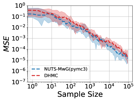
Figure 2: Mean Squared Error for the posterior estimates of the true posterior of the cluster means $\mu_{1:2}$. We compare the results from our unoptimized DHMC and the optimized PyMC3 NUTS with Metropolis-within-Gibbs, and show that the performance between the two is comparable for the same computation budget. The median of MSE (dashed lines) with $20\%/80\%$ confidence intervals (shaded regions) over $20$ independent runs are plotted.

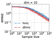
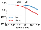
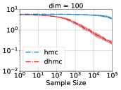
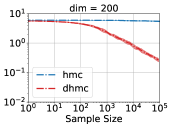
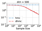
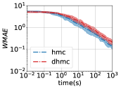
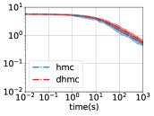
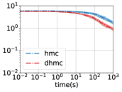
Figure 3: We compare DHMC against HMC on the worst mean absolute error (dashed lines) with the $20\%/80\%$ confidence intervals (shaded regions) over 20 independent runs for dimensions $D=10,50,100,200,500$ (left to right). We demonstrate how the sample efficiency decreases with respect to sample size (top row) and with respect to runtime (bottom row) respectively as dimensionality increases. We see that the performance of HMC deteriorates significantly more than DHMC as the dimensionality increases.

In our first example, we demonstrate how a classic model, namely a Gaussian mixture model, can be encoded in LF-PPL. The density of the GMM contains a mixture of continuous and discrete variables, where the discrete variables lead to discontinuities in the density. We construct the GMM as follows:

$$\mu_{k} \sim\mathcal{N}(\mu_{0},\sigma_{0}),\;k=1,\dots,K$$

$$z_{n} \sim\mathrm{Categorical}(p_{0}),\;n=1,\dots,N$$

$$y_{n}\,|z_{n},\, \mu_{z_{n}}\sim\mathcal{N}(\mu_{z_{n}},\sigma_{z_{n}}),\;n=1,\dots,N$$

where $\mu_{1:K},z_{1:N}$ are latent variables, $y_{1:N}$ are observed data with $K$ as the number of clusters and $N$ the total number of data. The Categorical distribution is constructed by a combination of uniform draws and nested if expressions, as shown in Appendix D. For our experiments, we considered a simple case with $\mu_{0}\,{=}\,0$, $\sigma_{0}\,{=}\,2$, $\sigma_{z_{1:N}}\,{=}\,1$ and $p_{0}\,{=}\,[0.5,0.5]$, along with the synthetic dataset: $y_{1:N}\,{=}\,[-2.0,-2.5,-1.7,-1.9,-2.2,1.5,2.2,3,1.2,2.8]$. We compared the Mean Squared Error (MSE) of the posterior estimates for the cluster means of both an unoptimized version of DHMC and an optimized implementation of NUTS with Metropolis-within-Gibbs (MwG) in PyMC3 [22], with the same computation budget. We take $10^{5}$ samples and discard $10^{4}$ for burn in. We find that our DHMC implementation, performs comparable to the NUTS with MwG approach. The results are shown in Figure 2 as a function of the number of samples.

6.2 Heavy Tail Piecewise Model

In our next example we show how the efficiency of DHMC improves, relative to vanilla HMC, on discontinuous target distributions as the dimensionality of the problem increases. We consider the following density[7] which represents a hyperbolic-like potential function,

$$\pi(\boldsymbol{x})=\begin{cases}\exp(-\sqrt{\boldsymbol{x}^{T}A\boldsymbol{x}})&\quad\text{if }||\boldsymbol{x}||_{\infty}\leq 3\\ \exp(-\sqrt{\boldsymbol{x}^{T}A\boldsymbol{x}}-1)&\quad\text{if }3<||\boldsymbol{x}||_{\infty}\leq 6\\ 0&\quad\text{otherwise}\end{cases}\vspace{-10pt}$$

It generates planes of discontinuities along the boundaries defined by the if expressions. To write this as a density in our language we make use of the factor distribution object as shown in Appendix D.

The results in Figure 3 provide a comparison between the DHMC and the standard HMC on the worst mean absolute error [7] as a function of the number of iterations and time, $\mathrm{WMAE}(N)=\frac{1}{N}\displaystyle\max_{d=1,\dots,D}\big{|}{\sum}_{n=1}^{N}\boldsymbol{x}_{d}^{(n)}\big{|}$. We see that as the dimensionality of the model increases, the per-sample performance of HMC deteriorates rapidly as seen in the top row of Figure 3. Even though DHMC is more expensive per iteration than HMC due to its sequential nature, in higher dimensions, the additional time costs occurred by DHMC is much less than the rate at which HMC performance deteriorates. The reason for this is that the acceptance rate of the HMC sampler degrades with increasing dimension, while the coordinate-wise integrator of the DHMC sampler circumvents this.

7 Conclusion

In this paper we have introduced a Low-level First-order Probabilistic Programming Language (LF-PPL) and an accompanying compilation scheme for programs that have non-differentiable densities. We have theoretically verified the language semantics via a series of translations rules. This ensures programs that compile in our language contain only discontinuities that are of measure zero. Therefore, our language together with the compilation scheme can be used in conjunction with other scalable inference algorithms such as adapted versions of HMC and SVI for non-differentiable densities, as we have demonstrated with one such variant of HMC called discontinuous HMC. It provides a road map for incorporating other inference algorithms into PPSs and shows the performance improvement of these inference algorithms over existing ones.

Acknowledgements

Yuan Zhou is sponsored by China Scholarship Council (CSC). Bradley Gram-Hansen is supported by the UK EPSRC CDT in Autonomous Intelligent Machines and Systems (CDT in AIMS). Tom Rainforth’s research leading to these results has received funding from the European Research Council under the European Union’s Seventh Framework Programme (FP7/2007-2013) ERC grant agreement no. 617071. Yang was supported by the Engineering Research Center Program through the National Research Foundation of Korea (NRF) funded by the Korean Government MSIT (NRF-2018R1A5A1059921), and also by Next-Generation Information Computing Development Program through the National Research Foundation of Korea (NRF) funded by the Ministry of Science, ICT (2017M3C4A7068177). Kohn and Wood were supported by DARPA D3M, Intel as part of the NERSC Big Data Center, and NSERC under its Discovery grant and accelerator programs.

Appendix A Proof of Theorem 1

Proof.

Assume that $\mathcal{P}$ is piecewise smooth under analytic partition. Thus,

$$\mathcal{P}(x)=\sum_{i=1}^{N}\prod_{j=1}^{M_{i}}\mathbbm{1}[p_{i,j}(x)\geq 0]\cdot\prod_{l=1}^{O_{i}}\mathbbm{1}[q_{i,l}(x)<0]\cdot h_{i}(x)$$ (2)

for some $N,M_{i},O_{i}$ and $p_{i,j},q_{i,l},h_{i}$ that satisfy the properties in Definition 1.

We use one well-known fact: the zero set $\{x\in\mathbb{R}^{n}\mid p(x)=0\}$ of an analytic function $p$ is the entire $\mathbb{R}^{n}$ or has zero Lebesgue measure [30]. We apply the fact to each $p_{i,j}$ and deduce that the zero set of $p_{i,j}$ is $\mathbb{R}^{n}$ or has measure zero. Note that if the zero set of $p_{i,j}$ is the entire $\mathbb{R}^{n}$, the indicator function $\mathbbm{1}[p_{i,j}\geq 0]$ becomes the constant-$1$ function, so that it can be omitted from the RHS of equation (2). In the rest of the proof, we assume that this simplification is already done so that the zero set of $p_{i,j}$ has measure zero for every $i,j$.

For every $1\leq i\leq N$, we decompose the $i$-th region

$$R_{i}=\{x\mid p_{i,j}\geq 0\ \mbox{and}\ q_{i,l}(x)<0\ \mbox{for all $j,l$}\}\,$$ (3)

to

$$\begin{array}[]{l}R^{\prime}_{i}=\{x\mid p_{i,j}>0\ \mbox{and}\ q_{i,l}(x)<0\ \mbox{for all $j,l$}\}\\[2.15277pt] R^{\prime\prime}_{i}=R_{i}\setminus R^{\prime}_{i}.\end{array}$$ (6)

Note that $R^{\prime}_{i}$ is open because the $p_{i,j}$ and $q_{i,l}$ are analytic and so continuous, both $\{r\in\mathbb{R}\mid r>0\}$ and $\{r\in\mathbb{R}\mid r<0\}$ are open, and the inverse images of open sets by continuous functions are open. This means that for each $x\in R^{\prime}_{i}$, we can find an open ball at $x$ inside $R^{\prime}_{i}$ so that $\mathcal{P}(x^{\prime})=h_{i}(x^{\prime})$ for all $x^{\prime}$ in the ball. Since $h_{i}$ is smooth, this implies that $\mathcal{P}$ is differentiable at every $x\in R^{\prime}_{i}$.

For the other part $R^{\prime\prime}_{i}$, we notice that

$$R^{\prime\prime}_{i}\subseteq\bigcup_{j=1}^{M_{i}}\{x\mid p_{i,j}(x)=0\}.$$

The RHS of this equation is a finite union of measure-zero sets, so it has measure zero. Thus, $R^{\prime\prime}_{i}$ also has measure zero as well.

Since $\{R_{i}\}_{1\leq i\leq N}$ is a partition of $\mathbb{R}^{n}$, we have that

$$\mathbb{R}^{n}=\bigcup_{i=1}^{N}R^{\prime}_{i}\cup\bigcup_{i=1}^{N}R^{\prime\prime}_{i}.$$

The density $\mathcal{P}$ is differentiable on the union of $R^{\prime}_{i}$’s. Also, since the union of finitely or countably many measure-zero sets has measure zero, the union of $R^{\prime\prime}_{i}$’s has measure zero. Thus, we can set the set $A$ required in the theorem to be this second union. ∎

Appendix B Proof of Theorem 2

Proof.

As shown in Equation 1,

$$\mathcal{P}\,{:=}\Big{(}\sum_{i=1}^{N_{D}}\eta_{i}{\cdot}k_{i}\Big{)}\cdot\Big{(}\sum_{j=1}^{N_{F}}\zeta_{j}{\cdot}l_{j}\Big{)}$$

it suffices to show that both factors are non-negative and piecewise smooth under analytic partition, because such functions are closed under multiplication.

We prove a more general result. For any expression $e$, let $\mathrm{Free}(e)$ be the set of its free variables. Also, if a function $\mathcal{G}$ in Definition 1 satisfies additionally that its $h_{i}$’s are analytic, we say that this function $\mathcal{G}$ is piecewise analytic under analytic partition. We claim that for all expressions $e$ (which may contain free variables), if $e\leadsto(\Delta,\Gamma,D,F)$, where $D=\{(\eta_{i},k_{i})\,|\,1{\leq}i{\leq}N_{D}\}$ and $F=\{(\zeta_{j},l_{j},v_{j})\,|\,1{\leq}j{\leq}N_{F}\}$, then $\Big{(}\sum_{i=1}^{N_{D}}\eta_{i}{\cdot}k_{i}\Big{)}$ and $\Big{(}\sum_{j=1}^{N_{F}}\zeta_{j}{\cdot}l_{j}\Big{)}$ are non-negative functions on variables in $\mathrm{Free}(e)\cup\Delta$ and they are piecewise analytic under analytic partition, as $k$ and $l^{\prime}$ in the sum are analytic. These two properties in turn imply that $\Big{(}\sum_{i=1}^{N_{D}}\eta_{i}{\cdot}k_{i}\Big{)}\cdot\Big{(}\sum_{j=1}^{N_{F}}\zeta_{j}{\cdot}l_{j}\Big{)}$ is a function on variables in $\mathrm{Free}(e)\cup\Delta$ and it is also piecewise analytic (and thus piecewise smooth) under analytic partition. Thus, the desired conclusion follows. Regarding our claim, we can prove it by induction on the structure of the expression $e$. ∎

Appendix C Discontinuous Hamiltonian Monte Carlo

The discontinuous HMC (DHMC) algorithm was proposed by [8]. It uses a coordinate-wise integrator, Algorithm 1, coupled with a Laplacian momentum to perform inference in models with non-differentiable densities. The algorithm works because the Laplacian momentum ensures that all discontinuous parameters move in steps of $\pm m_{b}\epsilon$ for fixed constants $m_{b}$ and step size $\epsilon$, where the index $b$ is associated to each discontinuous coordinate. These properties are advantages because they remove the need to know where the discontinuity boundaries between each region are; the change of the potential energy in the state before and after the $\pm m_{b}\epsilon$ move provides us with information of whether we have enough kinetic energy to move into this new region. If we do not have enough energy we reflect backwards $\mathbf{p}_{b}=-\mathbf{p}_{b}$. Otherwise, we move to this new region with a proposed coordinate update $\mathbf{x}_{b}^{*}$ and momentum $\mathbf{p}_{b}-m_{b}\cdot\mathit{sign}(\mathbf{p}_{b})\cdot\Delta U$. This is in contrast to algorithms such as Reflect, Refract HMC [7], that explictly need to know where the discontinuities boundaries are. Hence, it is important to have a compilation scheme that enables one to do that.

The addition of the random permutation $\phi$ of indices $b$ is to ensure that the coordinate-wise integrator satisfies the criterion of reversibility in the Hamiltonian. Although the integrator does not reproduce the exact solution, it nonetheless preserves the Hamiltonian exactly, even if the density is discontinuous. See Lemma 1 and Theorems 2-3 in [8]. This yields a rejection-free proposal.

Algorithm 1 Coordinate-wise Integrator. A random permutation $\phi$ on $\{1,\ldots,B\}$ is appropriate if the induced random sequences $(\phi(1),\ldots,\phi(|B|))$ and $(\phi(|B|),\ldots,\phi(1))$ have the same distribution

1:function Coordinatewise($\mathbf{x},\mathbf{p},\epsilon,U$)

2:     pick an appropriate random permutation $\phi$ on $B$

3:     for $i=1,\ldots,B$ do

4:         $b\leftarrow\phi(i)$

5:         $\mathbf{x}^{\ast}\leftarrow\mathbf{x}$

6:         $\mathbf{x}^{\ast}_{b}\leftarrow\mathbf{x}_{b}^{\ast}+\epsilon m_{b}\cdot\mathit{sign}(\mathbf{p}_{b})$

7:         $\Delta U\leftarrow U(\mathbf{x}^{\ast})-U(\mathbf{x})$

8:         if $K(\mathbf{p}_{b})=m_{b}|\mathbf{p}_{b}|>\Delta U$  then

9:              $\mathbf{x}_{b}\leftarrow\mathbf{x}_{b}^{\ast}$

10:              $\mathbf{p}_{b}\leftarrow\mathbf{p}_{b}-m_{b}\cdot\mathit{sign}(\mathbf{p}_{b})\cdot\Delta U$

11:         else

12:              $\mathbf{p}_{b}\leftarrow-\mathbf{p}_{b}$

13:         end if

14:     end for

15:     return ${\mathbf{x}_{b},\mathbf{p}_{b}}$

16:end function

Then DHMC algorithm [8] adpated for LF-PPL and our compilation scheme is as follows:

Algorithm 2 Discontinuous HMC Integrator for the LF-PPL.
$\chi$ is a map from random-variable names $n$ in $\Delta$ to their values $\mathbf{x}_{n}$, $H$ is the total Hamiltonian, $\epsilon>0$ is the step size, and $L$ is the trajectory length.

1:function DHMC-LFPPL($\Delta,\Gamma,D,F,\mathbf{x},\mathbf{p},H,\epsilon,L$)

2:     $B=\Gamma$;     $A=\Delta\setminus\Gamma$

3:     for $a\in A$ do $\triangleright$ $a$ represents the set of continuous variables

4:         $\mathbf{x}^{0}_{a}\leftarrow\mathbf{x}_{a}$;     $\mathbf{p}_{a}\sim\mathcal{N}(\mathbf{0},\mathbf{1})$

5:     end for

6:     for $b\in B$ do

7:         $\mathbf{x}^{0}_{b}\leftarrow\mathbf{x}_{b}$;     $\mathbf{p}_{b}\sim\mathit{Laplace}(\mathbf{0},\mathbf{1})$$\triangleright$ $b$ represents the set of discontinuous variables

8:     end for

9:     $\forall a\in A$, $\,\mathbf{x}^{0}_{a}\leftarrow\mathbf{x}_{a}$;     $\mathbf{p}_{a}\sim\mathcal{N}(\mathbf{0},\mathbf{1})$ $\triangleright$ $A$ represents the set of continuous variables

10:     $\forall b\in B$, $\,\mathbf{x}^{0}_{b}\leftarrow\,\mathbf{x}_{b}$;     $\mathbf{p}_{b}\sim\mathit{Laplace}(\mathbf{0},\mathbf{1})$$\triangleright$ $B$ represents the set of discontinuous variables

11:     $U\leftarrow-\mbox{\sc LogJointDensity}(D,F)$

12:     for $i=1$ to $L$ do

13:         $U_{A}\leftarrow U\ \mbox{with names in $B$ replaced by their values in $\mathbf{x}^{i}_{B}$}$

14:         $(\mathbf{x}^{i}_{A},\mathbf{p}^{i}_{A})\leftarrow$Halfstep1$(\mathbf{x}^{i-1}_{A},\mathbf{p}^{i-1}_{A},\epsilon,U_{A})$

15:         $U_{B}\leftarrow U\ \mbox{with names in $A$ replaced by their values in $\mathbf{x}^{i}_{A}$}$

16:         $(\mathbf{x}^{i}_{B},\mathbf{p}^{i}_{B})\leftarrow$Coordinate-wise($\mathbf{x}^{i-1}_{B},\mathbf{p}^{i-1}_{B},\epsilon,U_{B}$)

17:         $U_{A}\leftarrow U\ \mbox{with names in $B$ replaced by their values in $\mathbf{x}^{i}_{B}$}$

18:         $(\mathbf{x}^{i}_{A},\mathbf{p}^{i}_{A})\leftarrow$Halfstep2$(\mathbf{x}^{i}_{A},\mathbf{p}^{i}_{A},\epsilon,U_{A})$

19:     end for

20:     $\mathbf{x}^{L}\leftarrow\mathbf{x}^{L}_{A}\cup\mathbf{x}^{L}_{B}$, $\;\mathbf{p}^{L}\leftarrow\mathbf{p}^{L}_{A}\cup\mathbf{p}^{L}_{B}$;

21:     $\mathbf{x}^{*},\mathbf{p}^{*}\leftarrow\mbox{\sc Evaluate}(F,\;\mathbf{x}^{L},\mathbf{p}^{L})$

22:      $\alpha\sim Uniform(0,1)$

23:     if  $\alpha>\min\{1,\exp(H(\mathbf{x},\mathbf{p})-H(\mathbf{x}^{*},\mathbf{p}^{*}))\}$ then

24:         return $\mathbf{x}^{*},\mathbf{p}^{*}$

25:     else

26:         return $\mathbf{x},\mathbf{p}$

27:     end if

28:end function

29:function HALFSTEP1($\mathbf{x},\mathbf{p},\epsilon,U$)

30:     $\mathbf{p}^{\prime}\leftarrow\mathbf{p}-\frac{\epsilon}{2}\nabla_{\mathbf{x}}U(\mathbf{x})$

31:     $\mathbf{x}^{\prime}\leftarrow\mathbf{x}+\frac{\epsilon}{2}\nabla_{\mathbf{p}^{\prime}}K(\mathbf{p}^{\prime})$

32:     return ($\mathbf{x}^{\prime},\mathbf{p}^{\prime}$)

33:end function

34:function HALFSTEP2($\mathbf{x},\mathbf{p},\epsilon,U$)

35:     $\mathbf{x}^{\prime}\leftarrow\mathbf{x}+\frac{\epsilon}{2}\nabla_{\mathbf{p}}K(\mathbf{p})$

36:     $\mathbf{p}^{\prime}\leftarrow\mathbf{p}-\frac{\epsilon}{2}\nabla_{\mathbf{x^{\prime}}}U(\mathbf{x^{\prime}})$

37:     return ($\mathbf{x}^{\prime},\mathbf{p}^{\prime}$)

38:end function

Appendix D Program code

⬇

(let [y (vector -2.0 -2.5 ... 2.8)

pi [0.5 0.5]

z1 (sample (categorical pi))

...

z10(sample (categorical pi))

mu1 (sample (normal 0 2))

mu2 (sample (normal 0 2))

mus (vector mu1 mu2)]

(if (< (- z1) 0)

(observe (normal mu1 1) (nth y 0))

(observe (normal mu2 1) (nth y 0)))

...

(if (< (- z10) 0)

(observe (normal mu1 1) (nth y 9))

(observe (normal mu2 1) (nth y 9)))

(mu1 mu2 z1 ... z10))

figureThe LF-PPL version of the Gaussian mixture model detailed in Section 6.

⬇

(let [x (sample (uniform -6 6))

abs-x (max x (- x))

z (- (sqrt (* x (* A x))))]

(if (< (- abs-x 3) 0)

(observe (factor z) 0)

(observe (factor (- z 1)) 0))

x)

figureThe LF-PPL version of the heavy-tailed model detailed in Section 6.

References

- [1] H. Mohasel Afshar et al., “Probabilistic inference in piecewise graphical models,” 2016.
- [2] A. Gelman, H. S. Stern, J. B. Carlin, D. B. Dunson, A. Vehtari, and D. B. Rubin, Bayesian data analysis. Chapman and Hall/CRC, 2013.
- [3] A. D. Gordon, T. A. Henzinger, A. V. Nori, and S. K. Rajamani, “Probabilistic programming,” in Proceedings of the on Future of Software Engineering, pp. 167–181, ACM, 2014.
- [4] N. D. Goodman, V. K. Mansinghka, D. M. Roy, K. Bonawitz, and J. B. Tenenbaum, “Church: A Language for Generative Models,” in In UAI, pp. 220–229, 2008.
- [5] F. Wood, J. W. Meent, and V. Mansinghka, “A New Approach to Probabilistic Programming Inference,” in Artificial Intelligence and Statistics, 2014.
- [6] A. Gelman, D. Lee, and J. Guo, “Stan: A Probabilistic Programming Language for Bayesian Inference and Optimization,” Journal of Educational and Behavioral Statistics, vol. 40, no. 5, pp. 530–543, 2015.
- [7] H. M. Afshar and J. Domke, “Reflection, Refraction, and Hamiltonian Monte Carlo,” in Advances in Neural Information Processing Systems, pp. 3007–3015, 2015.
- [8] A. Nishimura, D. Dunson, and J. Lu, “Discontinuous Hamiltonian Monte Carlo for Sampling Discrete Parameters,” arXiv preprint arXiv:1705.08510, 2017.
- [9] W. Lee, H. Yu, and H. Yang, “Reparameterization gradient for non-differentiable models,” in NIPS, 2018.
- [10] V. Dinh, A. Bilge, C. Zhang, I. Matsen, and A. Frederick, “Probabilistic path hamiltonian monte carlo,” arXiv preprint arXiv:1702.07814, 2017.
- [11] K. Yi and F. Doshi-Velez, “Roll-back hamiltonian monte carlo,” arXiv preprint arXiv:1709.02855, 2017.
- [12] M. D. Hoffman, D. M. Blei, C. Wang, and J. Paisley, “Stochastic variational inference,” The Journal of Machine Learning Research, vol. 14, no. 1, pp. 1303–1347, 2013.
- [13] R. Ranganath, S. Gerrish, and D. Blei, “Black box variational inference,” in Artificial Intelligence and Statistics, pp. 814–822, 2014.
- [14] D. M. Blei, A. Kucukelbir, and J. D. McAuliffe, “Variational inference: A review for statisticians,” Journal of the American Statistical Association, vol. 112, no. 518, pp. 859–877, 2017.
- [15] A. Kucukelbir, R. Ranganath, A. Gelman, and D. Blei, “Automatic variational inference in stan,” in Advances in neural information processing systems, pp. 568–576, 2015.
- [16] S. Duane, A. D. Kennedy, B. J. Pendleton, and D. Roweth, “Hybrid Monte Carlo,” Physics letters B, 1987.
- [17] R. M. Neal, “MCMC Using Hamiltonian dynamics,” Handbook of Markov Chain Monte Carlo, 2011.
- [18] Y. Zhang, Z. Ghahramani, A. J. Storkey, and C. A. Sutton, “Continuous relaxations for discrete hamiltonian monte carlo,” in Advances in Neural Information Processing Systems, pp. 3194–3202, 2012.
- [19] A. Pakman and L. Paninski, “Auxiliary-variable exact hamiltonian monte carlo samplers for binary distributions,” in Advances in neural information processing systems, pp. 2490–2498, 2013.
- [20] A. Pakman and L. Paninski, “Exact hamiltonian monte carlo for truncated multivariate gaussians,” Journal of Computational and Graphical Statistics, vol. 23, no. 2, pp. 518–542, 2014.
- [21] A. G. Baydin, B. A. Pearlmutter, A. A. Radul, and J. M. Siskind, “Automatic differentiation in machine learning: a survey.,” Journal of machine learning research, vol. 18, no. 153, pp. 1–153.
- [22] J. Salvatier, T. V. Wiecki, and C. Fonnesbeck, “Probabilistic Programming in Python Using PyMC3,” PeerJ Computer Science, vol. 2, p. e55, 2016.
- [23] D. Tran, M. D. Hoffman, R. A. Saurous, E. Brevdo, K. Murphy, and D. M. Blei, “Deep probabilistic programming,” arXiv preprint arXiv:1701.03757, 2017.
- [24] H. Ge, K. Xu, and Z. Ghahramani, “Turing: Composable inference for probabilistic programming,” in International Conference on Artificial Intelligence and Statistics, AISTATS 2018, 9-11 April 2018, Playa Blanca, Lanzarote, Canary Islands, Spain, pp. 1682–1690, 2018.
- [25] UberLabs, “Pyro, a universal probabilistic programming language.” https://github.com/uber/pyro, 2017.
- [26] C. J. Maddison, A. Mnih, and Y. W. Teh, “The concrete distribution: A continuous relaxation of discrete random variables,” arXiv preprint arXiv:1611.00712, 2016.
- [27] D. Spiegelhalter, A. Thomas, N. Best, and W. Gilks, “BUGS 0.5: Bayesian Inference Using Gibbs Sampling Manual (version ii),” MRC Biostatistics Unit, Institute of Public Health, Cambridge, UK, pp. 1–59, 1996.
- [28] J.-W. van de Meent, B. Paige, H. Yang, and F. Wood, “An introduction to probabilistic programming,” arXiv preprint arXiv:1809.10756, 2018.
- [29] T. Rainforth, Automating Inference, Learning, and Design using Probabilistic Programming. PhD thesis.
- [30] B. Mityagin, “The Zero Set of a Real Analytic Function,” arXiv preprint arXiv:1512.07276, 2015.