Performance Analysis of Effective Symbolic Methods for Solving Band Matrix SLAEs

Abstract

This paper presents an experimental performance study of implementations of three symbolic algorithms for solving band matrix systems of linear algebraic equations with heptadiagonal, pentadiagonal, and tridiagonal coefficient matrices. The only assumption on the coefficient matrix in order for the algorithms to be stable is nonsingularity. These algorithms are implemented using the GiNaC library of C++ and the SymPy library of Python, considering five different data storing classes. Performance analysis of the implementations is done using the high-performance computing (HPC) platforms “HybriLIT” and “Avitohol”. The experimental setup and the results from the conducted computations on the individual computer systems are presented and discussed. An analysis of the three algorithms is performed.

1 Introduction

Systems of linear algebraic equations (SLAEs) with heptadiagonal (HD), pentadiagonal (PD) and tridiagonal (TD) coefficient matrices may arise after many different scientific and engineering problems, as well as problems of the computational linear algebra where finding the solution of a SLAE is considered to be one of the most important problems. On the other hand, special matrix’s characteristics like diagonal dominance, positive definiteness, etc.  are not always feasible. The latter two points explain why there is a need of methods for solving of SLAEs which take into account the band structure of the matrices and do not have any other special requirements to them. One possible approach to this problem is the symbolic algorithms. An overview of some of the symbolic algorithms which exist in the literature is done by us in [1]. What is common for all of them, is that they are implemented using Computer Algebra Systems (CASs) such as Maple, Mathematica, and Matlab.

Three direct symbolic algorithms for solving a SLAE based on LU decomposition are considered: for HD matrices (see [2] and [1]) – SHDM, for PD [3] – SPDM, and TD matrices [4] – STDM. The only assumption on the coefficient matrix is nonsingularity.

The choice of algorithms for solving problems of the computational linear algebra is crucial for the programs’ effectiveness, especially when these problems are with a big dimension. In that case they require the use of supercomputers and computer clusters for the solution to be obtained in a reasonable amount of time. Another important choice that has to be made and that influences the programs’ performance is what programming language to be used for the algorithms’ implementations. Here, we are going to focus on two of the most popular programming languages for scientific computations, namely C++ and Python. The aim of this paper, which is a logical continuation of [5] and [6], is to investigate the performance characteristics of the considered serial methods with their two implementations being executed on modern computer clusters.

2 Computational Experiments

Computations were held on the basis of the heterogeneous computational platform “HybriLIT” (1142 TFlops/s for single precision and 550 TFlops/s for double precision) [7] at the Laboratory of Information Technologies of the Joint Institute for Nuclear Research in the town of science Dubna, Russia, and on the cluster computer system “Avitohol” (412.3 TFlops/s for double precision) [8] at the Advanced Computing and Data Centre of the Institute of Information and Communication Technologies of the Bulgarian Academy of Sciences in Sofia, Bulgaria. The latter has been ranked among the TOP500 list (https://www.top500.org) twice – being 332nd in June 2015 and 388th in November 2015.

2.1 Experimental Setup

Table 1 sums up some basic information about hardware on the two computer systems, including models of processors, processors’ base frequency, and amount of cache memory (SmartCache). For even more information, visit: https://ark.intel.com/compare/75281,75269. Table 2 summarizes the basic information about the compilers and libraries used on the two computer systems. The three algorithms are implemented using the GiNaC library [9] of C++ [10] (the projects are built with the help of CMake [11]), and SymPy [12] library of Python [13] (using Anaconda distribution  [14]). The reason why optimization -O0 was used is that the GiNaC library is already optimized and any further attempts to optimize the code give worse results. Although we use Py 2.7, one should note that the implementations are fully compatible with Py 3.6 as well. It is worth mentioning that optimization attempts like autowrap and numba do not give better execution times. The former because of overhead, the second one because it cannot optimize further than what is already done.

Table 1: Intel processors used for numerical experiments.

Computer system	Processor	FREQ [GHz]	Cache [MB]
“HybriLIT”	Intel Xeon E5-2695v2	2.40	30
“Avitohol”	Intel Xeon E5-2650v2	2.60	20

Table 2: Information about the used software on the two computer systems.

Computer		“HybriLIT”	“Avitohol”
system
OS		Scientific Linux 7.4	Red Hat Linux
C++	Compilers	GCC (4.9.3)	GCC (6.2.0)
	Libraries	GiNaC (1.7.3)	GiNaC (1.7.2)
		CLN (1.3.4)
	Optimization	-O0
Python	Version	Anaconda (5.0.1): Py2.7
	Library	SymPy (1.1.1)

2.2 Experimental Results and Analysis of the Algorithms

During our experiments wall-clock times were collected and the average time from multiple runs is reported. For that purpose, we use std::chrono::high_resolution_clock::now() for C++ (requires at least standard c++11), and timeit.default_timer() for Python. Both of them provide the best clock rate available on the platform. Five different classes for data storing are tested – lst and matrix of GiNaC; Matrix (variable-size), Matrix (fixed-size), and MutableDenseNDimArray of SymPy. The first and the third are intended for variable-size storing, while the others – for fixed-size one (the SymPy’s Matrix could be both). Further we are going to denote the implementations of the three algorithms, using these 5 data storing classes as Impl. i, $i=\overline{1,\ldots 5}$. The notation is as follows: SXDM stands for symbolic X method, X $=$ HD, PD, TD. The achieved computational times from solving a SLAE are summarized in Tables 3–7.

Table 3: Results from solving a SLAE on the two clusters applying the first implementation.

	GiNaC (“lst” – var-size) := Impl. 1
	Wall-clock time [s]
	“HybriLIT”			“Avitohol”
$N$	SHDM	SPDM	STDM	SHDM	SPDM	STDM
$10^{3}$	0.191933	0.120892	0.054486	0.211552	0.108980	0.051806
$10^{4}$	29.346658	14.384663	6.4003244	30.525208	15.238341	5.280648
$10^{5}$	5095.508994	2389.583291	805.592624	4026.259486	2009.600485	711.940280

Table 4: Results from solving a SLAE on the two clusters applying the second implementation.

	GiNaC (“matrix” – fixed-size) := Impl. 2
	Wall-clock time [s]
	“HybriLIT”			“Avitohol”
$N$	SHDM	SPDM	STDM	SHDM	SPDM	STDM
$10^{3}$	0.025110	0.016281	0.008808	0.030020	0.017507	0.010651
$10^{4}$	0.254571	0.153711	0.086114	0.296938	0.173316	0.091560
$10^{5}$	2.567423	1.553468	0.858090	2.822281	1.694611	0.888428

Table 5: Results from solving a SLAE on the two clusters applying the third implementation.

	SymPy (“Matrix” – var-size) := Impl. 3
	Wall-clock time [s]
	“HybriLIT”			“Avitohol”
$N$	SHDM	SPDM	STDM	SHDM	SPDM	STDM
$10^{2}$	0.779426	0.541518	0.288752	1.198145	0.854763	0.450166
$10^{3}$	61.955375	47.205663	23.203961	102.278640	75.408729	36.983316
$10^{4}$	6159.227881	4587.017868	2294.136577	9967.937595	7517.447892	3751.046286

Table 6: Results from solving a SLAE on the two clusters applying the fourth implementation.

	SymPy (“Matrix” – fixed-size) := Impl. 4
	Wall-clock time [s]
	“HybriLIT”			“Avitohol”
$N$	SHDM	SPDM	STDM	SHDM	SPDM	STDM
$10^{3}$	0.875309	0.726237	0.417078	1.272449	0.788081	0.429694
$10^{4}$	8.420457	5.780376	2.909977	12.807111	7.738780	4.163307
$10^{5}$	84.977702	60.360366	29.446712	128.940536	77.026990	41.930210

Table 7: Results from solving a SLAE on the two clusters applying the fifth implementation.

	SymPy (“MutableDenseNDimArray” – fixed-size) := Impl. 5
	Wall-clock time [s]
	“HybriLIT”			“Avitohol”
$N$	SHDM	SPDM	STDM	SHDM	SPDM	STDM
$10^{3}$	0.730619	0.545021	0.308278	1.104916	0.694794	0.387745
$10^{4}$	7.472471	4.941960	3.115306	11.105768	6.726764	3.759721
$10^{5}$	73.927031	51.304943	30.917188	111.968824	67.404472	37.466753

Table 8: Estimation of the order $\alpha(10^{4},10^{5})$.

$\alpha(10^{4},10^{5})$
	“HybriLIT”					“Avitohol”
Impl.	#1	#2	#3	#4	#5	#1	#2	#3	#4	#5
SHDM	2.24	1.00	2.00	1.00	1.00	2.12	0.98	1.99	1.00	1.00
SPDM	2.22	1.00	1.99	1.02	1.02	2.12	0.99	2.00	1.00	1.00
STDM	2.10	1.00	2.00	1.01	1.00	2.13	0.99	2.01	1.00	1.00

Using the following formula ($k$ – unknown coefficient of proportionality, $t_{i}$ – time, $N_{i}$ – the matrix’s number of rows, $i=1,2$):

$$t\approx kN^{\alpha}\quad\Rightarrow\quad\frac{t_{2}}{t_{1}}=\left(\frac{N_{2}}{N_{1}}\right)^{\alpha}\quad\Leftrightarrow\quad\alpha(N_{1},N_{2})=\dfrac{\log(t_{2})-\log(t_{1})}{\log(N_{2})-\log(N_{1})},$$

the order of growth of execution time $\alpha$ for all the five implementations was estimated (see Table 8).

Remark: The number of needed operations for Gaussian elimination so as a HD SLAE to be transformed into a PD one is $35N-122$, while the number of needed operations so as a PD SLAE to be transformed into a TD one is $23N-52$, where $N$ is the matrix’s number of rows. This observation is relevant to Figure 1 which depicts the factors of time growth HD:TD, PD:TD, TD:TD for each of the implementations.

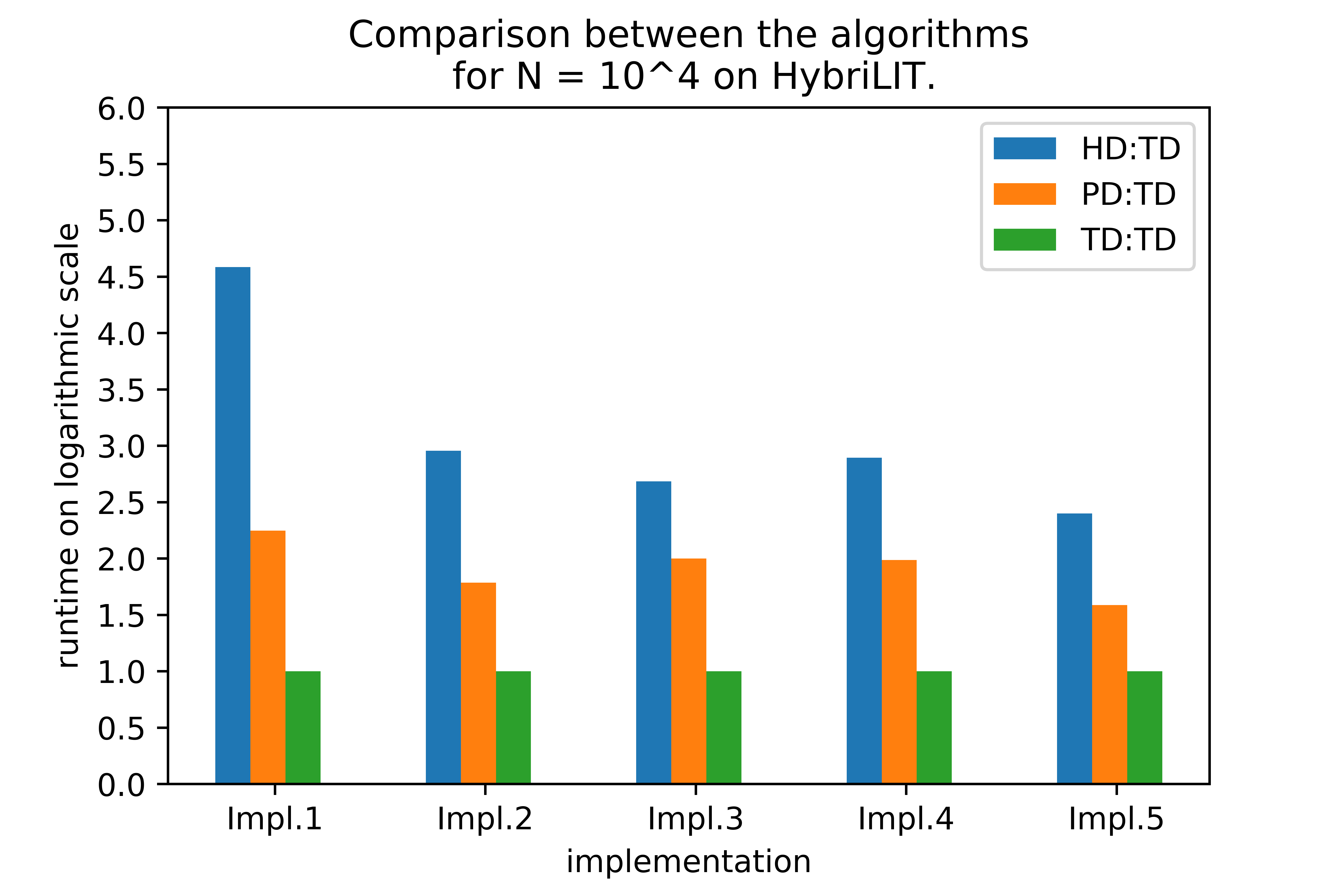
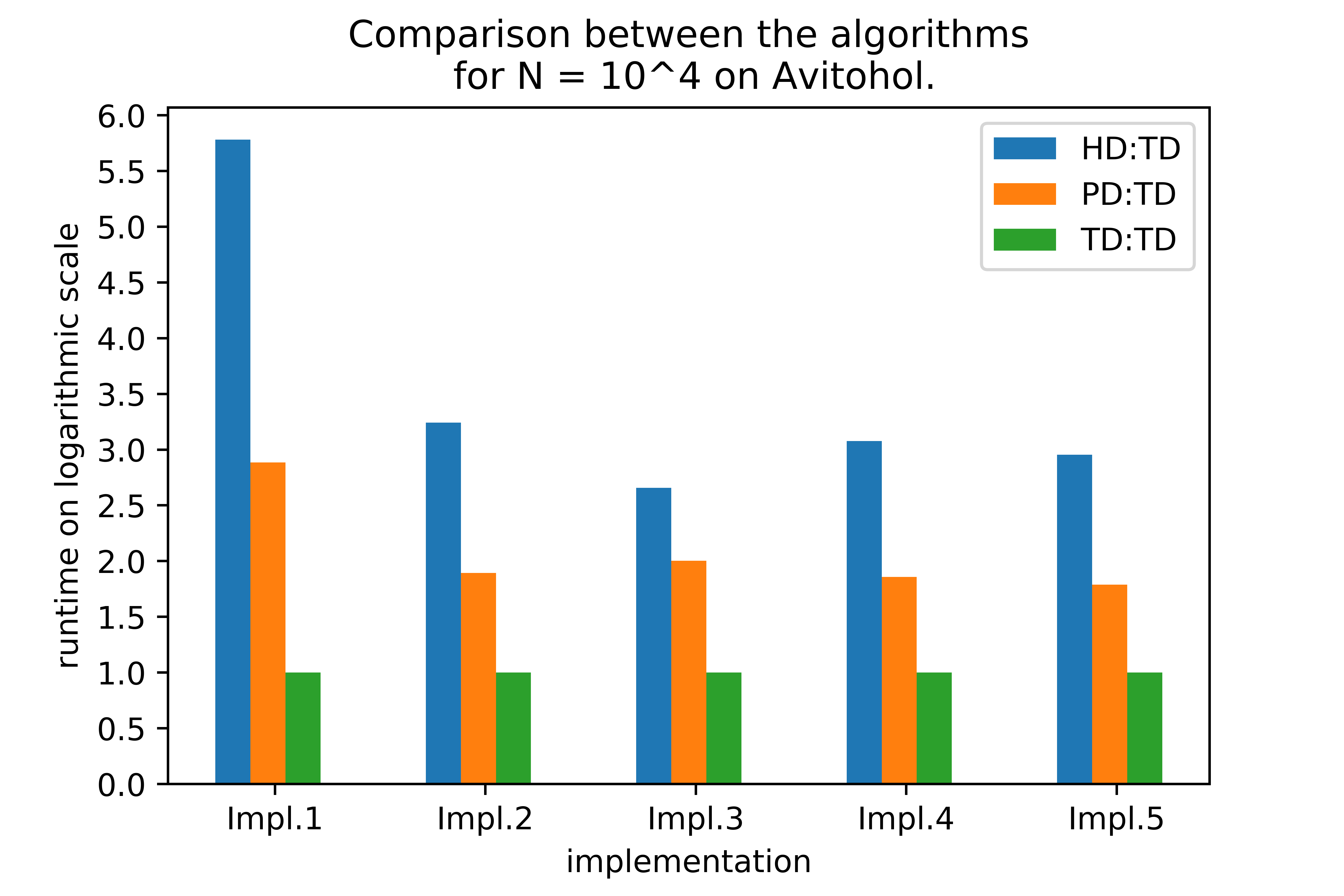
Figure 1: Comparison between the algorithms for $N=10^{4}$.

3 Discussion and Conclusions

Direct comparison between the five implementations shows that the best GiNaC one is Impl. 2, while the best SymPy one is Impl. 5 (see Figure 2). Expectedly, the GiNaC implementations of the three algorithms yield a much better computation time in comparison with the respected SymPy implementations with the difference being between one and two orders of magnitude. It must be mentioned that the matrix class in SymPy is a subclass of the ndarray. This means that every call on a matrix object requires a few extra Python calls. This usually leads to a little slower performance although the difference is negligible. Figures 3 and 4 depict a comparison of the execution time of the best GiNaC and SymPy implementations on the two clusters. As one can see, “HybriLIT” behaves better than “Avitohol” with the difference being bigger when the SymPy is of interest. It is obvious that the implementations which rely on variable-size storing classes (that are Impl. 2 and Impl.3) were found to be much slower than the ones which use fixed-size storing classes, but while this was expected, it does not belittle their importance since there is a class of problems where the size of the matrix is unknown at runtime.

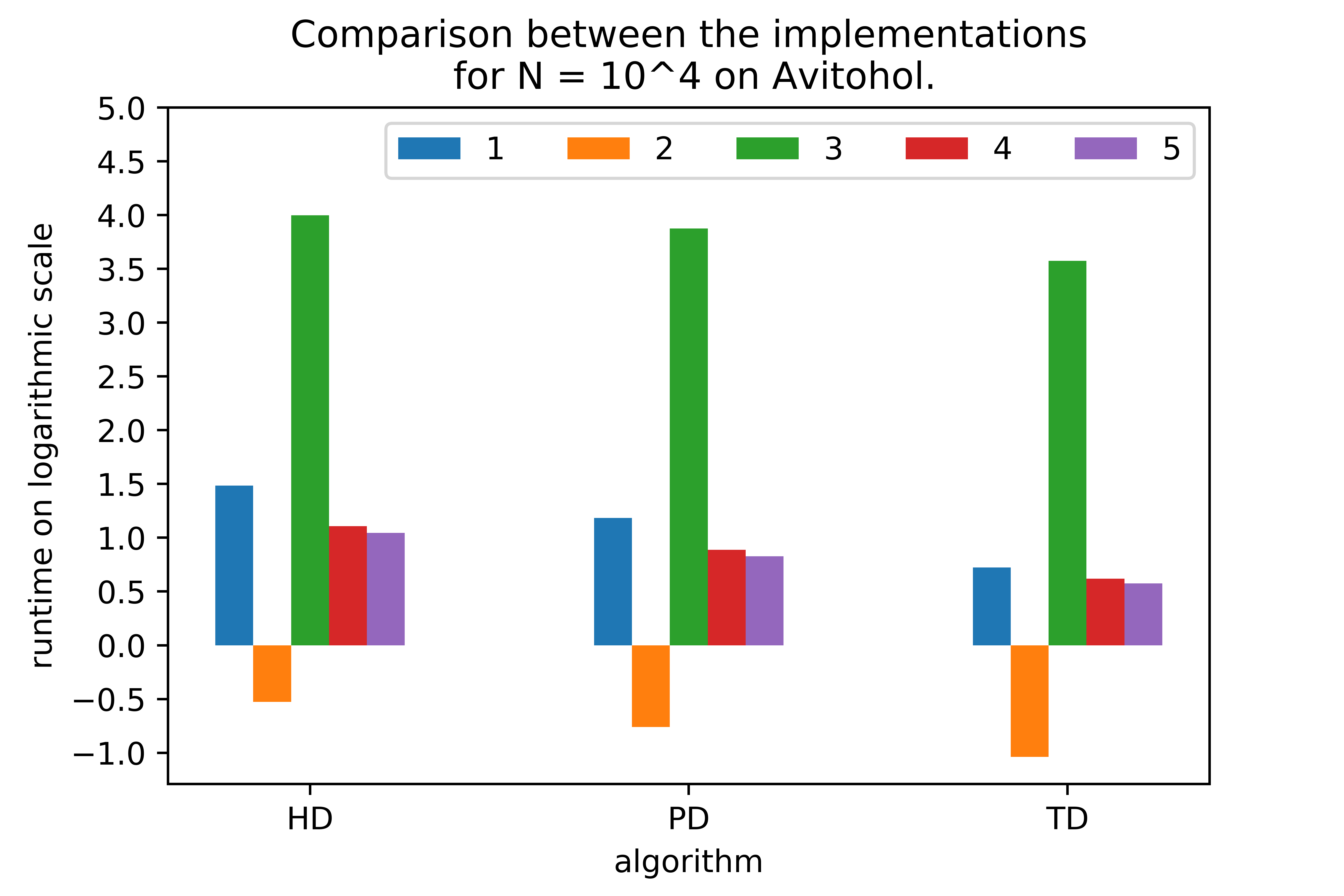
Figure 2: Comparison between the implementations for $N=10^{4}$.

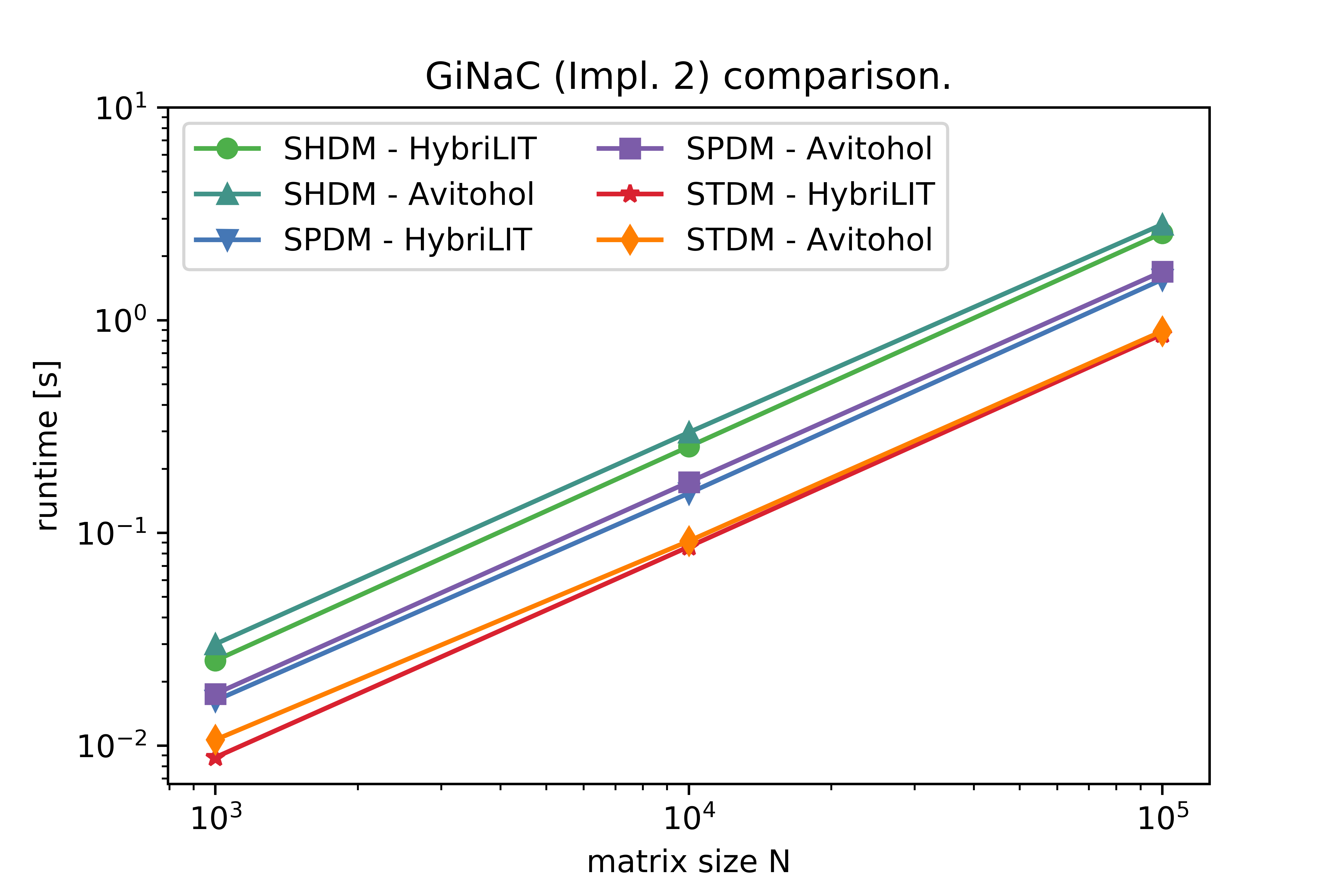
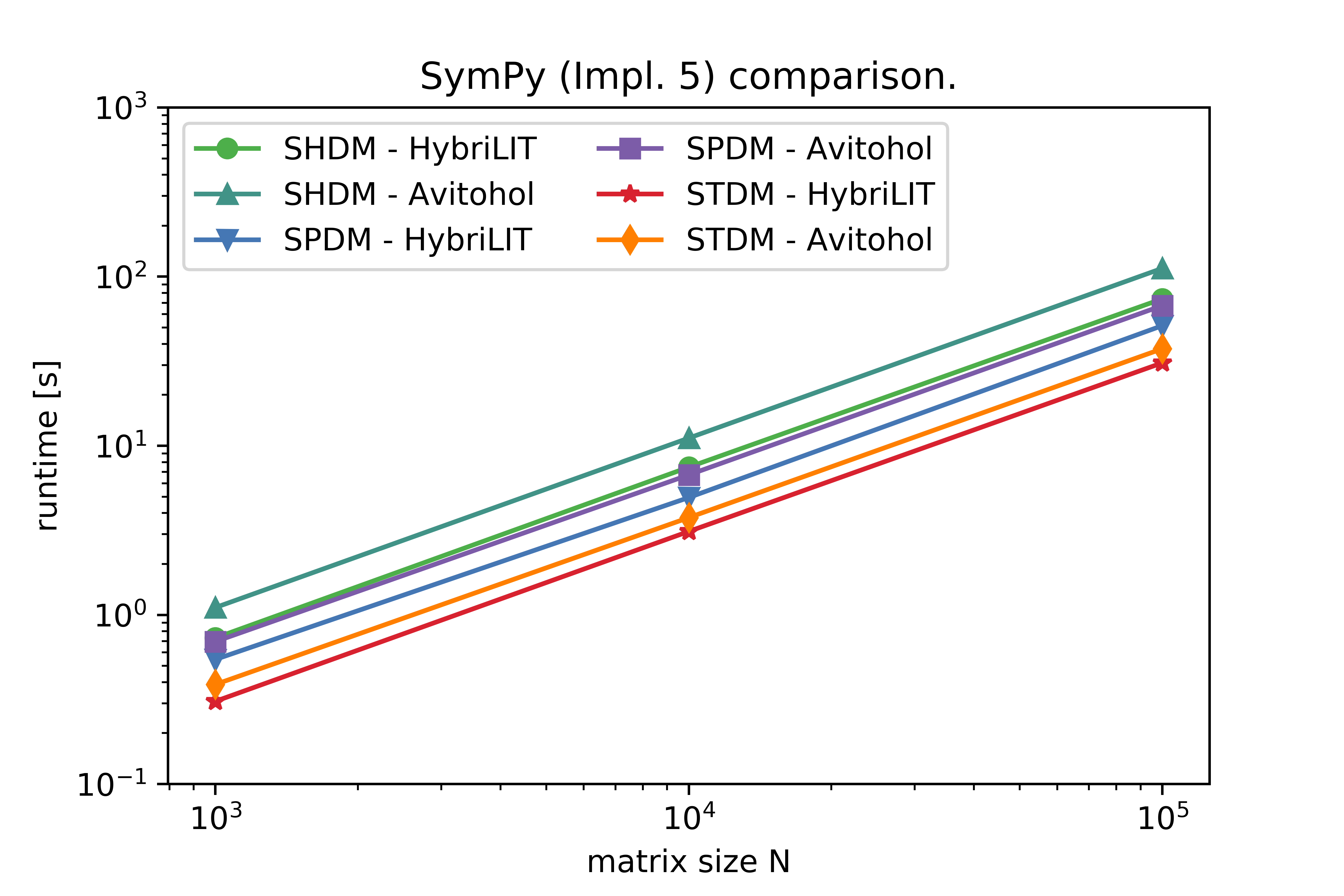
Figure 3: Comparison of the execution time of the best GiNaC and SymPy implementations on the two clusters.

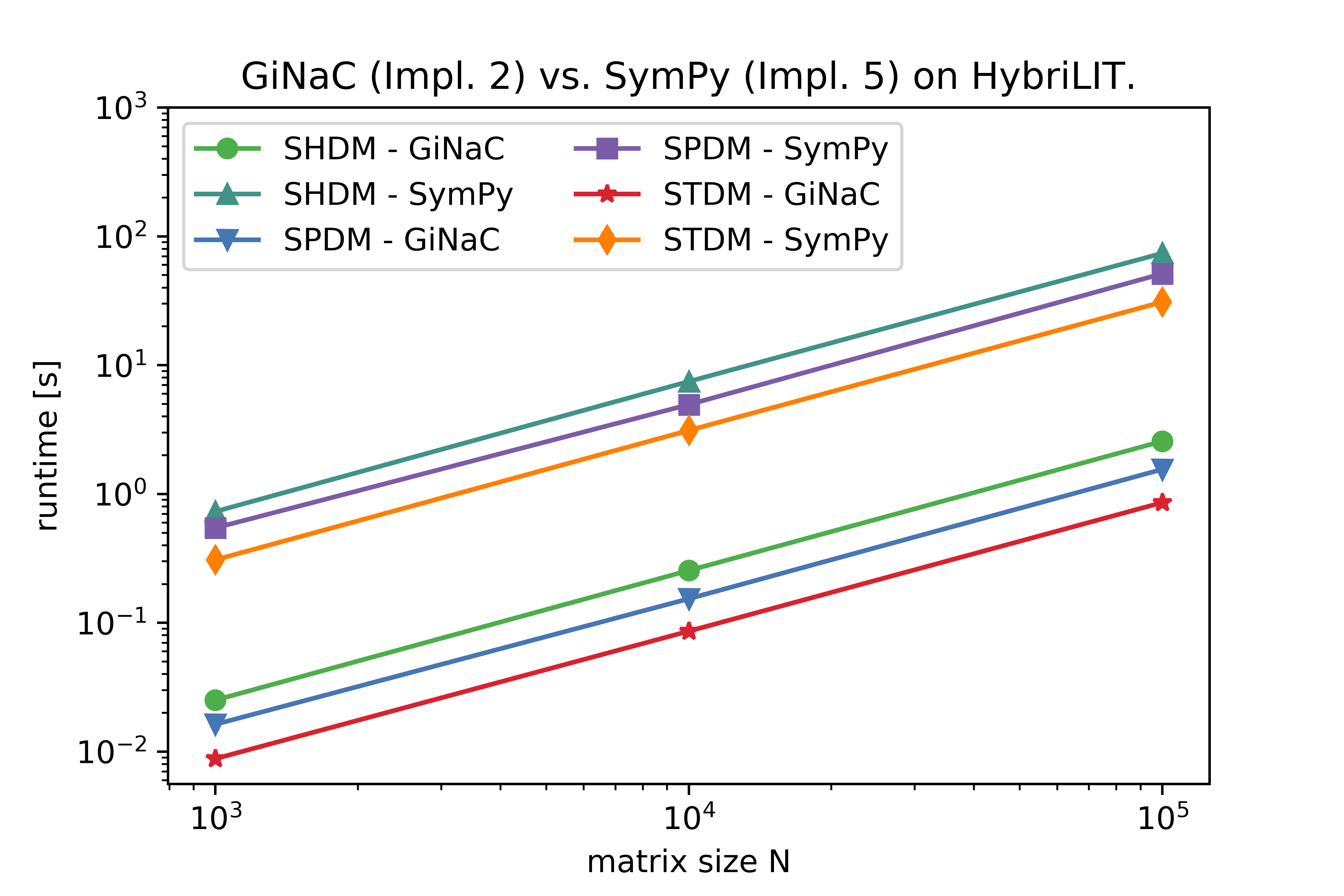
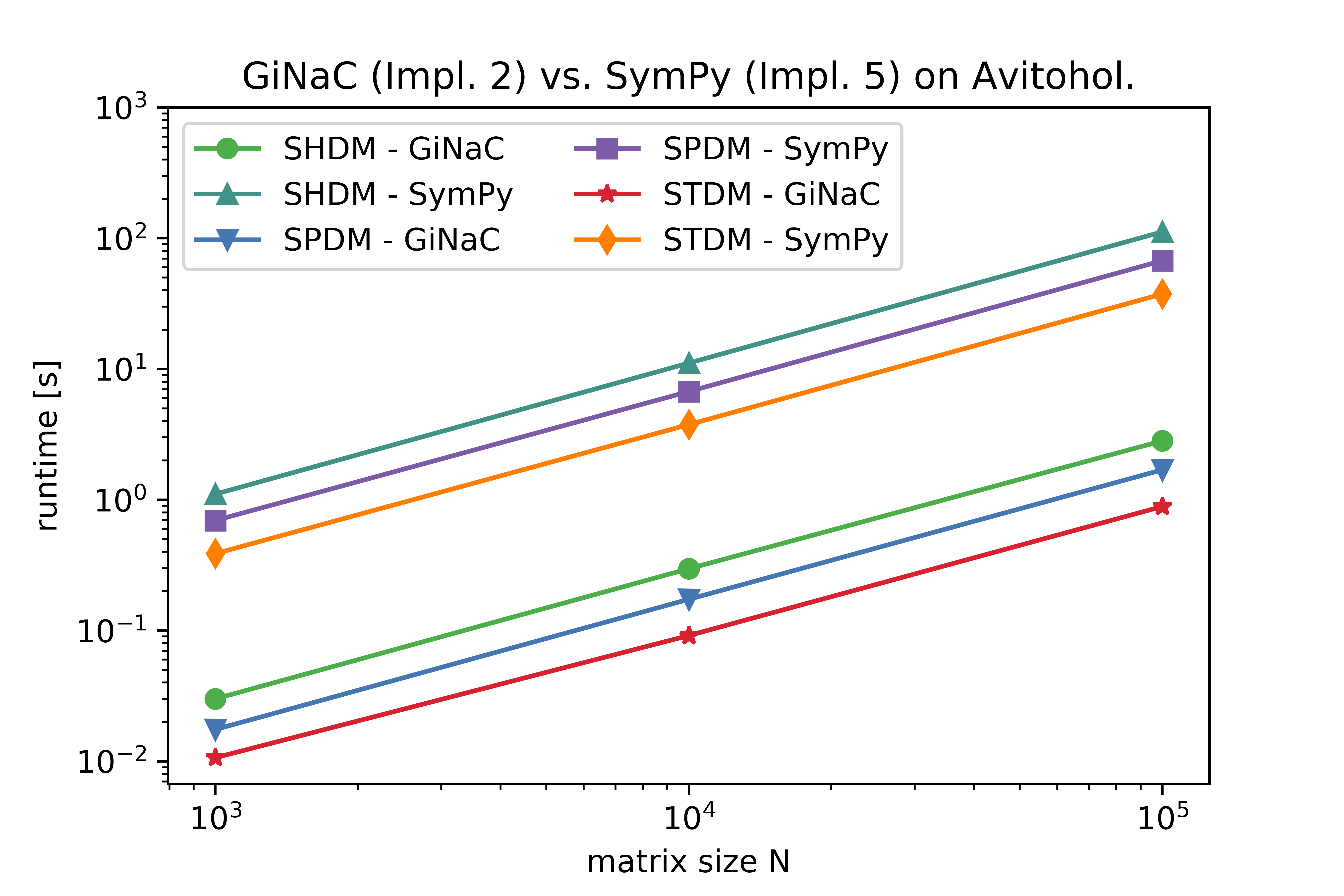
Figure 4: Comparison of the execution time of the best GiNaC and SymPy implementations on the two clusters.

As it can be seen in Table 9, three of the implementations have a linear time growth, while the other two have a quadratic trend. Theoretically, all the algorithms introduced here have a linear complexity. This means that even if theoretically the execution time has to grow as $O(N)$, the two implementations which rely on variable-size storing classes show time growth as $O(N^{2})$, with Impl. 1 even having $\alpha>2$. Hence, the variable-size of the storing class changes the order of complexity with one order of magnitude.

Table 9: Order of time growth.

Order of growth	Implementation
$O(N)$	2, 4, 5
$O(N^{2})$	1, 3

The choice of a programming language depends on a lot of factors. However, in the context of symbolic computations for solving a SLAE with a band coefficient matrix (length of band equal to 3, 5 or 7) among the options suggested in this work, we can note the following: Python is easier to learn and easier and faster to prototype (no need for memory management, build systems, compilers, etc.), on the other hand, C++ has better performance and occupies less memory, but requires much more attention to bookkeeping and storage details.

References

- [1] Veneva, M., Ayriyan, A.: Symbolic Algorithm for Solving SLAEs with Heptadiagonal Coefficient Matrices. Mathematical Modelling and Geometry, 6, 3, 22–29 (2018).
- [2] Karawia, A. A.: A New Algorithm for General Cyclic Heptadiagonal Linear Systems Using Sherman-Morrisor-Woodbury Formula. ARS Combinatoria, 108, 431–443 (2013).
- [3] Askar, S. S., Karawia, A. A.: On Solving Pentadiagonal Linear Systems via Transformations. Mathematical Problems in Engineering. Hindawi Publishing Corporation. 2015, 9 (2015), doi: 10.1155/2015/232456.
- [4] El-Mikkawy, M.: A Generalized Symbolic Thomas Algorithm. Applied Mathematics. 3, 4, 342–345 (2012), doi: 10.4236/am.2012.34052.
- [5] Veneva, M., Ayriyan, A.: Effective Methods for Solving Band SLAEs after Parabolic Nonlinear PDEs. AYSS-2017, European Physics Journal – Web of Conferences (EPJ-WoC). 177, 07004 (2018).
- [6] Veneva, M., Ayriyan, A.: Performance Analysis of Effective Methods for Solving Band Matrix SLAEs after Parabolic Nonlinear PDEs. Advanced Computing in Industrial Mathematics, Revised Selected Papers of the 12th Annual Meeting of the Bulgarian Section of SIAM, December 20–22, 2017, Sofia, Bulgaria, Studies in Computational Intelligence, 793, 407–419 (2019), doi: 10.1007/978-3-319-97277-0_33.
- [7] Adam, Gh., Bashashin, M., Belyakov, D., Kirakosyan, M., Matveev, M., Podgainy, D., Sapozhnikova, T., Streltsova, O., Torosyan, Sh., Vala, M., Valova, L., Vorontsov, A., Zaikina, T., Zemlyanaya, E., Zuev, M.: IT-ecosystem of the HybriLIT Heterogeneous Platform for High-performance Computing and Training of IT-specialists. Selected Papers of the 8th International Conference “Distributed Computing and Grid-technologies in Science and Education” (GRID 2018), Dubna, Russia, September 10–14, 2018, 2267, 638–644.
- [8] Supercomputer System Avitohol at IICT-BAS, http://www.hpc.acad.bg/.
- [9] Bauer, C., Frink, A., Kreckel, R.: Introduction to the GiNaC Framework for Symbolic Computation within the C++ Programming Language. J. Symbolic Computation. 33, 1–12 (2002), doi: 10.1006/jsco.2001.0494.
- [10] ISO/IEC. (2012). ISO International Standard ISO/IEC for Programming Language C++. [Working draft], N3337. Geneva, Switzerland: International Organization for Standardization (ISO). Retrieved from https://isocpp.org/std/the-standard.
- [11] CMake. The Cross Platform Build System. Kitware Inc. (2018), https://cmake.org.
- [12] Meurer, A., Smith, C. P., Paprocki, M., Čertík, O., Kirpichev, S. B., Rocklin, M., Kumar, A., Ivanov, S., Moore, J. K., Singh, S., Rathnayake, T., Vig, S., Granger, B. E., Muller, R. P., Bonazzi, F., Gupta, H., Vats, S., Johansson, F., Pedregosa, F., Curry, M. J., Terrel, A. R., Roučka, Š., Saboo, A., Fernando, I., Kulal, S., Cimrman, R., Scopatz, A.: SymPy: Symbolic Computing in Python. PeerJ Computer Science. 3, e103 (2017), doi: 10.7717/peerj-cs.103.
- [13] Python Core Team (2015). Python: A Dynamic, Open Source Programming Language. Python Software Foundation, https://www.python.org/.
- [14] Anaconda Software Distribution. Computer Software. Anaconda (2018), https://anaconda.com.
- [15] Hunter, J. D.: Matplotlib: A 2D Graphics Environment. Computing in Science & Engineering. 9, 3, 90–95 (2007), doi: 10.1109/MCSE.2007.55.