Convergence of the light-front coupled-cluster method in quenched scalar Yukawa theory

Abstract

We explore the convergence of the light-front coupled-cluster (LFCC) method in the context of two-dimensional quenched scalar Yukawa theory. This theory is simple enough for higher-order LFCC calculations to be relatively straightforward. The quenching is to maintain stability; the spectrum of the full theory with pair creation and annihilation is unbounded from below. The basic interaction in the quenched theory is only emission and absorption of a neutral scalar by the complex scalar. The LFCC method builds the eigenstate with one complex scalar and a cloud of neutrals from a valence state that is just the complex scalar and the action of an exponentiated operator that creates neutrals. The lowest order LFCC operator creates one; we add the next order, a term that creates two. At this order there is a direct contribution to the wave function for two neutrals and one complex scalar and additional contributions to all higher Fock wave functions from the exponentiation. Results for the lowest order and this new second-order approximation are compared with those obtained with standard Fock-state expansions. The LFCC approach is found to allow representation of the eigenstate with far fewer functions than the number of wave functions required in a converged Fock-state expansion.

I Introduction

The calculation of the bound states for a given quantum field theory is an inherently nonperturbative problem. Various methods can be applied, the best known being, of course, lattice (gauge) theory lattice . Here we consider a method based on a Hamiltonian formulation in light-front coordinates Dirac ; LFreviews . The fundamental bound-state problem is then the eigenvalue problem

$${\cal P}^{-}|\psi(\underline{P})\rangle=\frac{M^{2}+P_{\perp}^{2}}{P^{+}}|\psi(\underline{P}\rangle,$$ (1)

where ${\cal P}^{-}$ is the light-front Hamiltonian, $M$ is the mass of the eigenstate, and $\underline{P}=(P^{+},\vec{P}_{\perp})$ is the light-front momentum. The Hamiltonian is constructed from the Lagrangian ${\cal L}$ for a generic field $\phi$ as

$${\cal P}^{-}=\int dx^{-}d^{2}x_{\perp}\left[:\frac{\delta{\cal L}}{\delta(\partial_{+}\phi)}-{\cal L}:\right]_{x^{+}=0}.$$ (2)

The eigenstate $|\psi(\underline{P})\rangle$ has definite momentum $\underline{P}$, and, once known, can be used to compute properties of the state This formulation is particularly convenient for the computation of form factors, because $|\psi(\underline{P})\rangle$ is boost invariant.

The standard approach to the solution of the eigenvalue problem is to write the eigenstate as a Fock-state expansion, which leads to a coupled system of equations for the Fock wave functions. This coupled system is then converted into a matrix eigenvalue problem, either by direct discretization, as in discrete light-cone quantization (DLCQ) PauliBrodsky , or by basis function expansion, as in basis light-front quantization (BLFQ) Vary . However, a finite matrix representation requires a truncation of the Fock space.

This truncation has serious consequences. In particular, there can be uncanceled divergences, and self-energy corrections become dependent on the Fock sector and on the presence of spectator constituents. These are the nonperturbative analog of what would happen to the contribution from a Feynman diagram if the diagram were decomposed into the various time orderings, with the removal of the time orderings that involve too many intermediates. These difficulties led to the idea of sector-dependent renormalization PerryWilson ; HillerBrodsky ; Karmanov , which has its own difficulties SecDep .

As an alternative, we have developed the light-front coupled-cluster (LFCC) method LFCC . No Fock-space truncation is invoked. Instead, the eigenstate is written as coming from the action of an exponentiated operator $T$ acting on a valence state $|\phi(\underline{P})\rangle$

$$|\psi(\underline{P})\rangle=\sqrt{Z}e^{T}|\phi(\underline{P})\rangle,$$ (3)

with $\sqrt{Z}$ a normalization factor. The valence state is something simple that carries all the appropriate quantum numbers, in addition to the total momentum; for a proton in QCD it would be the three-quark state. The operator $T$ increases particle number in various ways and conserves all the quantum numbers of the valence state; in QCD, $T$ would include gluon emission from a quark or gluon and pair creation from a gluon.

The original eigenvalue problem is converted into two parts, through multiplication by $e^{-T}$ and projection onto the valence sector and its complement. To express this, we define the effective Hamiltonian $\overline{{\cal P}^{-}}\equiv e^{-T}{\cal P}^{-}e^{T}$ and the projection $P_{v}$ onto the valence sector. We then have

$$P_{v}\overline{{\cal P}^{-}}|\phi(\underline{P})\rangle=\frac{M^{2}+P_{\perp}^{2}}{P^{+}}|\phi(\underline{P})\rangle,\;\;(1-P_{v})\overline{{\cal P}^{-}}|\phi(\underline{P})\rangle=0.$$ (4)

Roughly speaking, the first equation determines $M$ and any wave functions in $|\phi\rangle$, while the second determines the functions that define the structure of $T$. In reality, of course, they are a coupled system, unless the valence state has a single constituent and therefore no wave functions.

All of this is obviously more complicated than the original eigenvalue problem, but it is exact. The power of the approach comes from the approximation step: Rather than truncate Fock space, we truncate $T$. Even for the simplest $T$ operator, its exponentiation allows the eigenstate to span an infinite Fock space, and, without much difficulty, one can arrange the approximate $e^{T}|\phi\rangle$ to fully explore all Fock sectors relevant for the quantum numbers of the valence state. In terms of a Fock-state expansion, what we have done is to force the wave functions of the higher Fock sectors to be directly dependent on those of the lower sectors rather than setting these higher wave functions to zero, as would happen in a Fock-space truncation. Yet another way to interpret the LFCC approximation is that the eigenstate is represented by a generalized coherent state. In any case, the avoidance of a Fock-space truncation eliminates the sector dependence and spectator dependence of self-energy corrections and potentially controls the uncanceled divergences.

The LFCC equations themselves are also truncated. The complement projection $1-P_{v}$ is restricted to the lowest set of Fock sectors necessary to have enough equations to solve for the functions that define $T$. This means that the LFCC method is not variational; the effective Hamiltonian $\overline{{\cal P}^{-}}$ is not Hermitian, and the truncated projections are not equivalent to minimization of the expectation value $\langle\psi|{\cal P}^{-}|\psi\rangle$.

One price to be paid for the gains of the LFCC method is that the LFCC equations are nonlinear. The existence of a solution can be difficult to guarantee. However, a linearized perturbative solution shows that the LFCC equations re-sum perturbation theory to all orders for a restricted set of diagrams. (The restriction arises because of the truncation of $T$.) This implies that, for weak coupling, a physical solution must exist. Depending on the structure chosen for $T$ and $|\phi\rangle$, the physical solution may disappear as the coupling is increased. An explicit example of this appears in an application to $\phi^{4}$ theory LFCCphi4 , where the solution for the lowest-order approximation for $T$ does not extend beyond a certain coupling strength. This is likely due to the restriction of the valence state to a single constituent in a regime near the critical coupling where all Fock sectors should contribute strongly.

One question that immediately arises has to do with the convergence of the method, in the sense that as one relaxes the truncations of $T$ and $1-P_{v}$, how does the solution improve? The present work answers this question in a particular context, with an application to quenched scalar Yukawa theory WC in two dimensions. In general, the correspondence between perturbation theory and the LFCC resummation at weak coupling shows that the convergence of the LFCC method is closely related to the convergence of perturbation theory at weak coupling. To get beyond weak coupling, we compare a nonperturbative Fock-state expansion calculation to LFCC calculations done with $T$ operators of increasing complexity.

The quenching of the theory eliminates potential concerns about the vacuum. Recent work BCH ; Collins ; Martinovic ; ETtoLF ; Katz has emphasized the need for care in considering the vacuum on the light front, but here no vacuum bubbles can occur. This also means that the Fock wave functions of a massive state do not include vacuum contributions and therefore have a direct physical interpretation. This is not generally true in equal-time quantization, where one must compute the vacuum state as well as massive states; as an example, see the work on $\phi^{4}$ theory by Rychkov and Vitale RychkovVitale .

The Lagrangian, Hamiltonian, and Fock-state expansion for quenched scalar Yukawa theory are given in Sec. II. The formulation of the LFCC method for this theory is developed in Sec. III. The results for both the Fock-state expansion method and the LFCC method are presented and compared in Sec. IV, with a brief summary provided in Sec. V. Details of numerical methods and diagrammatic rules are left to appendices.

II Quenched scalar Yukawa theory

The Lagrangian for scalar Yukawa theory WC is

$${\cal L}=|\partial_{\mu}\chi|^{2}-m^{2}|\chi|^{2}+\frac{1}{2}(\partial_{\mu}\phi)^{2}-\frac{1}{2}\mu^{2}\phi^{2}-g\phi|\chi|^{2},$$ (5)

where $\chi$ is a complex scalar field with mass $m$ and $\phi$ is a real scalar field with mass $\mu$. The two fields are coupled by a Yukawa term with strength $g$. In two dimensions, the light-front Hamiltonian density is

$${\cal H}=m^{2}|\chi|^{2}+\frac{1}{2}\mu^{2}\phi^{2}+g\phi|\chi|^{2}.$$ (6)

The mode expansions for the fields are

$$\chi = \int\frac{dp}{\sqrt{4\pi p}}\left[c_{+}(p)e^{-ipx^{-}/2}+c_{-}^{\dagger}(p)e^{ipx^{-}/2}\right],$$ (7)

$$\phi = \int\frac{dp}{\sqrt{4\pi p}}\left[a(p)e^{-ipx^{-}/2}+a^{\dagger}(p)e^{ipx^{-}/2}\right].$$ (8)

The nonzero commutation relations of the creation and annihilation operators are

$$[c_{\pm}(p),c^{\dagger}_{\pm}(p^{\prime})]=\delta(p-p^{\prime}),\;\;[a(p),a^{\dagger}(p^{\prime})]=\delta(p-p^{\prime}).$$ (9)

In terms of these operators, the quenched light-front Hamiltonian ${\cal P}^{-}=\int dx^{-}{\cal H}={\cal P}^{-}_{0}+{\cal P}^{-}_{\rm int}$ is specified by

$${\cal P}^{-}_{0}=\int dp\frac{m^{2}}{p}\left[c_{+}^{\dagger}(p)c_{+}(p)+c_{-}^{\dagger}(p)c_{-}(p)+a^{\dagger}(p)a(p)\right]$$ (10)

and

$${\cal P}^{-}_{\rm int}=g\int\frac{dpdq}{\sqrt{4\pi pq(p+q)}}\left\{\left[c_{+}^{\dagger}(p+q)c_{+}(p)+c_{-}^{\dagger}(p+q)c_{-}(p)\right]a(q)+{\rm h.c.}\right\}.$$ (11)

Pair creation and annihilation terms are suppressed, to stabilize the spectrum.

We seek eigenstates of ${\cal P}^{-}$, for which the two-dimensional light-front mass eigenvalue problem is

$${\cal P}^{-}|\psi(P)\rangle=\frac{M^{2}}{P}|\psi(P)\rangle.$$ (12)

We limit this to the charge-one sector. In the next section, we consider the LFCC approach to the solution of this eigenvalue problem, but here we develop the standard Fock-state expansion approach, to use as a basis for comparison.

We write the Fock-state expansion of the eigenstate as

$$|\psi(P)\rangle=\sum_{n=0}^{\infty}P^{n/2}\int\left(\prod_{i=1}^{n}dx_{i}\right)\theta(1-\sum_{i}x_{i})\psi_{n}(x_{1},\ldots,x_{n})\frac{1}{\sqrt{n!}}\prod_{i}a^{\dagger}(x_{i}P)c_{+}^{\dagger}((1-\sum_{i}x_{i})P)|0\rangle.$$ (13)

Projection of the eigenvalue problem onto $\prod_{j}^{n^{\prime}}a^{\dagger}(y_{j}P)c_{+}^{\dagger}((1-\sum_{j}^{n^{\prime}}y_{i})P)|0\rangle$, and division by $\mu^{2}$, yields coupled equations for the Fock-state wave functions $\psi_{n}$

$$\left[\frac{\tilde{m}^{2}}{1-\sum_{j}y_{j}}+\sum_{j}\frac{1}{y_{j}}\right]\psi_{n}(y_{1},\ldots,y_{n})+\frac{\lambda}{\sqrt{n}}\sum_{j}^{n}\frac{\psi_{n-1}(y_{1},\ldots,y_{j-1},y_{j+1},\ldots,y_{n})}{\sqrt{y_{j}(1-\sum_{i\neq j}y_{i})(1-\sum_{i}^{n}y_{i})}}$$

$$+\lambda\sqrt{n+1}\int dx\,\theta(1-x-\sum_{i}y_{i})\frac{\psi_{n+1}(y_{1},\ldots,y_{n},x)}{\sqrt{x(1-x-\sum_{i}y_{i})(1-\sum_{i}y_{i})}}=\frac{M^{2}}{\mu^{2}}\psi_{n}(y_{1},\ldots,y_{n}).$$

Here $\tilde{m}\equiv m/\mu$ is a dimensionless relative mass and $\lambda\equiv g/(\sqrt{4\pi}\mu^{2})$ is a dimensionless coupling strength. We solve this system numerically by first truncating the Fock space at $n=n_{\rm max}$ neutrals and expanding the wave functions in a symmetrized monomial basis. The details are discussed in Appendix A, and the results in Sec. IV.

The structure of the eigenstate is studied by considering the relative probabilities for Fock sectors with different numbers of neutrals. These are formed as the ratio

$$R_{n}\equiv\frac{1}{\psi_{0}^{2}}\int\prod_{i}dx_{i}\,\theta(1-\sum_{i}x_{i})|\psi_{n}|^{2}.$$ (15)

Results for these ratios are shown in Sec. IV.

III Light-front coupled-cluster method

The LFCC method constructs the charge-one eigenstate in the form

$$|\psi\rangle=\sqrt{Z}e^{T}c_{+}^{\dagger}|0\rangle,$$ (16)

where $c_{+}^{\dagger}|0\rangle$ is the single-particle valence state. The $T$ operator is expanded in a sequence $T=\sum_{n}T_{n}$, with

$$T_{n}=\int\prod_{i}^{n}dx_{i}dp\,p^{n/2}t_{n}(x_{1},\ldots,x_{n})\prod_{i}^{n}a^{\dagger}(x_{i}p)c_{+}^{\dagger}((1-\sum_{i}^{n}x_{i})p)c_{+}(p).$$ (17)

The factor $p^{n/2}$ is included to keep $T_{n}$ dimensionless; $p$ is the natural scale, being the momentum flowing through the operator.

The action of $T_{n}$ is to increase the number of neutrals by $n$, and the exponentiation of $T$ provides for generation of all possible (quenched) charge-one Fock states, even if $T$ is truncated to only $T_{1}$. Without truncation, the functions $t_{n}$ provide for an exact solution, with a duality between the $t_{n}$ and the Fock-state wave functions $\psi_{n}$. However, without truncation the eigenvalue problem is equivalent to an infinite coupled system of nonlinear equations for these $t_{n}$.

We can then study the convergence of the LFCC method as the number of terms in $T$ is increased. Here we consider the first two terms, $T_{1}$ and $T_{2}$, and compare results with those from the truncated Fock-state expansion.

The LFCC form of the eigenvalue problem is

$$P_{v}\overline{{\cal P}^{-}}c_{+}^{\dagger}(P)|0\rangle=\frac{M^{2}}{P}c_{+}^{\dagger}(P)|0\rangle,\;\;(1-P_{v})\bar{\cal P}^{-}c_{+}^{\dagger}(P)|0\rangle=0.$$ (18)

Independent of the level of truncation for $T$, the first equation becomes

$$\frac{m^{2}}{P}c_{+}^{\dagger}(P)|0\rangle+\frac{g}{\sqrt{4\pi}}\int\frac{dq}{\sqrt{(P-q)qP}}\frac{t_{1}(q/P)}{\sqrt{P}}c_{+}^{\dagger}(P)|0\rangle=\frac{M^{2}}{P}c_{+}^{\dagger}(P)|0\rangle.$$ (19)

The contributions to this equation come from the ${\cal P}^{-}_{0}$ and ${\cal P}^{-}_{\rm int}T_{1}$ terms in $\overline{{\cal P}^{-}}$, as represented diagrammatically in Fig. 1.

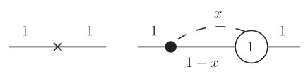
Figure 1: Diagrammatic representation of the valence equation. Rules for diagrams are given in Appendix B.

On division by $\mu^{2}$, the projected valence equation reduces to the following expression for the eigenmass $M$:

$$\frac{M^{2}}{\mu^{2}}=\tilde{m}^{2}+\lambda\int\frac{dx\,t_{1}(x)}{\sqrt{x(1-x)}}\equiv\tilde{m}^{2}+\lambda\Delta.$$ (20)

The self-energy term is then specified by

$$\Delta=\int\frac{dx\,t_{1}(x)}{\sqrt{x(1-x)}}.$$ (21)

The function $t_{1}$ is to be obtained by solving the remaining LFCC equations.

With each truncation of $T$ there is a matching truncation of the projector $1-P_{v}$ to include only enough Fock sectors to determine the unknown functions in the retained terms of $T$. Given the truncation to $T=T_{1}+T_{2}$, the equations for $t_{1}$ and $t_{2}$ take the form of two projections, onto the sectors with one and two neutrals. The contributions to the first projection come from

$$\overline{{\cal P}^{-}}\rightarrow{\cal P}^{-}_{\rm int}+{\cal P}^{-}_{0}T_{1}-T_{1}{\cal P}^{-}_{0}-T_{1}{\cal P}^{-}_{\rm int}T_{1}+\frac{1}{2}{\cal P}^{-}_{\rm int}T_{1}^{2}+{\cal P}^{-}_{\rm int}T_{2}.$$ (22)

These terms are represented in Fig. 2

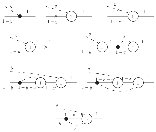
Figure 2: Diagrammatic representation of the projection onto the one-neutral Fock sector.

and yield the following equation for $t_{1}$:

$$0 = \frac{\lambda}{\sqrt{y(1-y)}}+\left[\frac{\tilde{m}^{2}}{1-y}+\frac{1}{y}-\tilde{m}^{2}\right]t_{1}(y)-\lambda t_{1}(y)\int_{0}^{1}\frac{dx\,t_{1}(x)}{\sqrt{x(1-x)}}$$

$$+\frac{1}{2}\frac{\lambda}{1-y}t_{1}(y)\int_{0}^{1-y}\frac{dx\,t_{1}(\frac{x}{1-y})}{\sqrt{x(1-y-x)}}+\frac{1}{2}\frac{\lambda}{\sqrt{1-y}}\int_{0}^{1-y}\frac{dx\,t_{1}(\frac{y}{1-x})t_{1}(x)}{\sqrt{x(1-x)(1-y-x)}}$$

$$+\frac{2\lambda}{\sqrt{1-y}}\int_{0}^{1-y}\frac{dx\,t_{2}(y,x)}{\sqrt{x(1-y-x)}}.$$

The equation (III) for $t_{1}$ can be obtained either by explicitly carrying out the contractions of annihilation and creation operators or by diagrammatic rules listed in Appendix B.

The first term in the second line of Eq. (III) can be simplified by rescaling the integration variable $x$ by $1-y$; this shows the integral to be equal to $\Delta$. The same self-energy integral appears in the last term of the first line. The terms proportional to $\Delta$ can then be collected with the $\tilde{m}$ terms, to introduce $M^{2}$ with use of (20)

$$\left[\frac{M^{2}}{\mu^{2}}-\frac{M^{2}/\mu^{2}}{1-y}-\frac{1}{y}\right]t_{1}(y) = \frac{\lambda}{\sqrt{y(1-y)}}+\frac{2\lambda}{\sqrt{1-y}}\int_{0}^{1-y}\frac{dx\,t_{2}(y,x)}{\sqrt{x(1-y-x)}}$$

$$+\frac{1}{2}\frac{\lambda}{\sqrt{1-y}}\left[\int_{0}^{1-y}\frac{dx\,t_{1}(\frac{y}{1-x})t_{1}(x)}{\sqrt{x(1-x)(1-y-x)}}-\frac{\Delta}{\sqrt{1-y}}t_{1}(y)\right].$$

For the truncation $T=T_{1}$, this equation, with the $t_{2}$ term removed, is all that need be solved.

The appearance of the physical mass $M$ in the invariant-mass terms on the left of (III) is typical of the LFCC method, where self-energy corrections are independent of the Fock sector and independent of spectators. This avoids the use of the sector-dependent bare masses that are frequently introduced in truncated Fock-state-expansion calculations PerryWilson ; HillerBrodsky ; Karmanov ; SecDep , where self-energy corrections are sector and spectator dependent.

The contributions to the second projection, onto the two-neutral sector, come from the following terms in $\overline{{\cal P}^{-}}$:

$$\overline{{\cal P}^{-}} \rightarrow {\cal P}^{-}_{0}T_{2}-T_{2}{\cal P}^{-}_{0}+\frac{1}{2}{\cal P}^{-}_{0}T_{1}^{2}-T_{1}{\cal P}^{-}_{0}T_{1}+\frac{1}{2}T_{1}^{2}{\cal P}^{-}_{0}+{\cal P}^{-}_{\rm int}T_{1}-T_{1}{\cal P}^{-}_{\rm int}$$

$$+\frac{1}{6}{\cal P}^{-}_{\rm int}T_{1}^{3}-\frac{1}{2}T_{1}{\cal P}^{-}_{\rm int}T_{1}^{2}+\frac{1}{2}T_{1}^{2}{\cal P}^{-}_{\rm int}T_{1}+\frac{1}{2}{\cal P}^{-}_{\rm int}T_{1}T_{2}+\frac{1}{2}{\cal P}^{-}_{\rm int}T_{2}T_{1}-T_{1}{\cal P}^{-}_{\rm int}T_{2}-T_{2}{\cal P}^{-}_{\rm int}T_{1}.$$

Graphical representations of these terms are given in Figs. 3-7. They and the rules in Appendix B yield the equation for $t_{2}$ as

$$0 = 2\left[\frac{\tilde{m}^{2}}{1-y_{1}-y_{2}}+\frac{1}{y_{1}}+\frac{1}{y_{2}}-\tilde{m}^{2}\right]t_{2}(y_{1},y_{2})$$

$$+\frac{1}{2}\frac{t_{1}(\frac{y_{2}}{1-y_{1}})t_{1}(y_{1})}{y_{1}\sqrt{1-y_{1}}}+\frac{1}{2}\frac{t_{1}(\frac{y_{1}}{1-y_{2}})t_{1}(y_{2})}{y_{2}\sqrt{1-y_{2}}}+\frac{1}{2}\frac{t_{1}(\frac{y_{2}}{1-y_{1}})t_{1}(y_{1})}{y_{2}\sqrt{1-y_{1}}}+\frac{1}{2}\frac{t_{1}(\frac{y_{1}}{1-y_{2}}t_{1}(y_{2})}{y_{1}\sqrt{1-y_{2}}}$$

$$+\frac{1}{2}\frac{\tilde{m}^{2}t_{1}(\frac{y_{2}}{1-y_{1}})t_{1}(y_{1})}{(1-y_{1}-y_{2})\sqrt{1-y_{1}}}+\frac{1}{2}\frac{\tilde{m}^{2}t_{1}(\frac{y_{1}}{1-y_{2}})t_{1}(y_{2})}{(1-y_{1}-y_{2})\sqrt{1-y_{2}}}$$

$$-\frac{\tilde{m}^{2}t_{1}(\frac{y_{2}}{1-y_{1}})t_{1}(y_{1})}{(1-y_{1})^{3/2}}-\frac{\tilde{m}^{2}t_{1}(\frac{y_{1}}{1-y_{2}})t_{1}(y_{2})}{(1-y_{2})^{3/2}}-\frac{t_{1}(\frac{y_{2}}{1-y_{1}})t_{1}(y_{1})}{y_{1}\sqrt{1-y_{1}}}-\frac{t_{1}(\frac{y_{1}}{1-y_{2}})t_{1}(y_{2})}{y_{2}\sqrt{1-y_{2}}}$$

$$+\frac{1}{2}\frac{\tilde{m}^{2}t_{1}(\frac{y_{2}}{1-y_{1}})t_{1}(y_{1})}{\sqrt{1-y_{1}}}+\frac{1}{2}\frac{\tilde{m}^{2}t_{1}(\frac{y_{1}}{1-y_{2}})t_{1}(y_{2})}{\sqrt{1-y_{2}}}$$

$$+\frac{\lambda t_{1}(y_{1})}{\sqrt{y_{2}(1-y_{1})(1-y_{1}-y_{2})}}+\frac{\lambda t_{1}(y_{2})}{\sqrt{y_{1}(1-y_{2})(1-y_{1}-y_{2})}}$$

$$-\lambda\frac{t_{1}(\frac{y_{2}}{1-y_{1}})}{(1-y_{1})\sqrt{y_{1}}}-\lambda\frac{t_{1}(\frac{y_{1}}{1-y_{2}})}{(1-y_{2})\sqrt{y_{2}}}$$

$$+\frac{1}{6}\left[\int_{0}^{1-y_{1}-y_{2}}dx\frac{\lambda t_{1}(\frac{y_{2}}{1-y_{1}-x})t_{1}(\frac{y_{1}}{1-x})t_{1}(x)}{\sqrt{x(1-x)(1-y_{1}-y_{2})(1-y_{1}-x)(1-y_{1}-y_{2}-x)}}+(y_{1}\leftrightarrow y_{2})\right]$$

$$+\frac{1}{6}\left[\int_{0}^{1-y_{1}-y_{2}}dx\frac{\lambda t_{1}(\frac{y_{2}}{1-y_{1}-x})t_{1}(\frac{x}{1-y_{1}})t_{1}(y_{1})}{\sqrt{x(1-y_{1})(1-y_{1}-y_{2})(1-y_{1}-x)(1-y_{1}-y_{2}-x)}}+(y_{1}\leftrightarrow y_{2})\right]$$

$$+\frac{1}{6}\left[\int_{0}^{1-y_{1}-y_{2}}dx\frac{\lambda t_{1}(\frac{x}{1-y_{1}-y_{2}})t_{1}(\frac{y_{2}}{1-y_{1}})t_{1}(y_{1})}{(1-y_{1}-y_{2})\sqrt{x(1-y_{1})(1-y_{1}-y_{2}-x)}}+(y_{1}\leftrightarrow y_{2})\right]$$

$$-\frac{1}{2}\left[\int_{0}^{1-y_{1}}dx\frac{\lambda t_{1}(\frac{y_{2}}{1-y_{1}})t_{1}(\frac{x}{1-y_{1}})t_{1}(y_{1})}{(1-y_{1})^{3/2}\sqrt{x(1-y_{1}-x)}}+(y_{1}\leftrightarrow y_{2})\right]$$

$$-\frac{1}{2}\left[\int_{0}^{1-y_{1}}dx\frac{\lambda t_{1}(\frac{y_{2}}{1-y_{1}})t_{1}(\frac{y_{1}}{1-x})t_{1}(x)}{(1-y_{1})\sqrt{x(1-x)(1-y_{1}-x)}}+(y_{1}\leftrightarrow y_{2})\right]$$

$$+\frac{1}{2}\left[\int_{0}^{1}dx\frac{\lambda t_{1}(\frac{y_{2}}{1-y_{1}})t_{1}(y_{1})t_{1}(x)}{\sqrt{x(1-x)(1-y_{1})}}+(y_{1}\leftrightarrow y_{2})\right].$$

$$+\int_{0}^{1-y_{1}-y_{2}}dx\frac{\lambda t_{2}(\frac{y_{1}}{1-x},\frac{y_{2}}{1-x})t_{1}(x)}{(1-x)\sqrt{x(1-y_{1}-y_{2})(1-y_{1}-y_{2}-x)}}$$

$$+\left[\int_{0}^{1-y_{1}-y_{2}}dx\frac{\lambda t_{2}(\frac{x}{1-y_{1}},\frac{y_{2}}{1-y_{1}})t_{1}(y_{1})}{(1-y_{1})\sqrt{x(1-y_{1}-y_{2})(1-y_{1}-y_{2}-x)}}+(y_{1}\leftrightarrow y_{2})\right]$$

$$+\int_{0}^{1-y_{1}-y_{2}}dx\frac{\lambda t_{1}(\frac{x}{1-y_{1}-y_{2}})t_{2}(y_{1},y_{2})}{(1-y_{1}-y_{2})\sqrt{x(1-y_{1}-y_{2}-x)}}$$

$$+\left[\int_{0}^{1-y_{1}-y_{2}}dx\frac{\lambda t_{1}(\frac{y_{2}}{1-y_{1}-x})t_{2}(y_{1},x)}{\sqrt{x(1-y_{1}-x)(1-y_{1}-y_{2})(1-y_{1}-y_{2}-x)}}+(y_{1}\leftrightarrow y_{2})\right]$$

$$-2\left[\int_{0}^{1-y_{1}}dx\frac{\lambda t_{1}(\frac{y_{2}}{1-y_{1}})t_{2}(y_{1},x)}{(1-y_{1})\sqrt{x(1-y_{1}-x)}}+(y_{1}\leftrightarrow y_{2})\right]-2\int_{0}^{1}dx\frac{\lambda t_{2}(y_{1},y_{2})t_{1}(x)}{\sqrt{x(1-x)}}.$$

We solve these equations numerically, as discussed in Appendix A, both for $t_{1}$ alone and the coupled system, for $t_{1}$ and $t_{2}$.

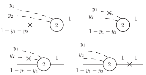
Figure 3: Diagrammatic representation of the projection onto the two-neutral Fock sector of the $\overline{{\cal P}^{-}}$ terms ${\cal P}^{-}_{0}T_{2}-T_{2}{\cal P}^{-}_{0}$.

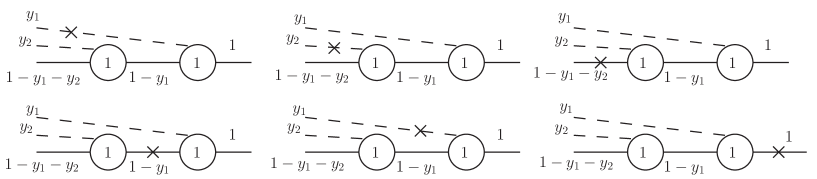
Figure 4: Same as Fig. 3 but for the $\overline{{\cal P}^{-}}$ terms $\frac{1}{2}{\cal P}^{-}_{0}T_{1}^{2}-T_{1}{\cal P}^{-}_{0}T_{1}+\frac{1}{2}T_{1}^{2}{\cal P}^{-}_{0}$.

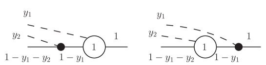
Figure 5: Same as Fig. 3 but for the $\overline{{\cal P}^{-}}$ terms ${\cal P}^{-}_{\rm int}T_{1}-T_{1}{\cal P}^{-}_{\rm int}$.

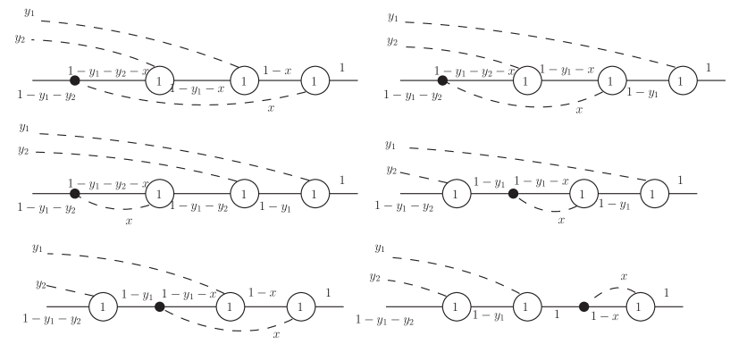
Figure 6: Same as Fig. 3 but for the $\overline{{\cal P}^{-}}$ terms $\frac{1}{6}{\cal P}^{-}_{\rm int}T_{1}^{3}-\frac{1}{2}T_{1}{\cal P}^{-}_{\rm int}T_{1}^{2}+\frac{1}{2}T_{1}^{2}{\cal P}^{-}_{\rm int}T_{1}$.

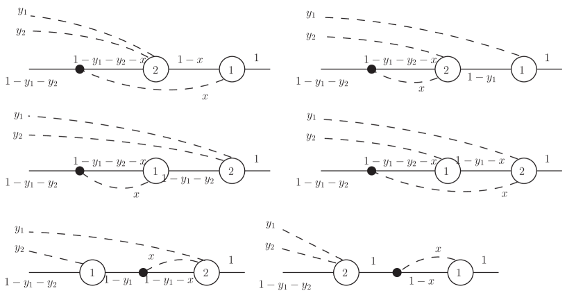
Figure 7: Same as Fig. 3 but for the $\overline{{\cal P}^{-}}$ terms $\frac{1}{2}{\cal P}^{-}_{\rm int}T_{1}T_{2}+\frac{1}{2}{\cal P}^{-}_{\rm int}T_{2}T_{1}-T_{1}{\cal P}^{-}_{\rm int}T_{2}-T_{2}{\cal P}^{-}_{\rm int}T_{1}$.

The relative probabilities for different Fock sectors can be computed from the expansion of the exponential form of the LFCC approximation

$$|\psi\rangle=\sqrt{Z}e^{T_{1}+T_{2}}c_{+}^{\dagger}(P)|0\rangle\simeq\sqrt{Z}\left[1+T_{1}+(T_{2}+\frac{1}{2}T_{1}^{2})+\cdots\right]c_{+}^{\dagger}(P)|0\rangle.$$ (27)

The Fock state wave functions can be extracted by comparison with the Fock state expansion in (13), after the actions of the operators $T_{1}$ and $T_{2}$ are taken into account. We find $\psi_{0}=\sqrt{Z}$, $\psi_{1}(x)=\sqrt{Z}t_{1}(x)$, and

$$\psi_{2}(x_{1},x_{2})=\sqrt{\frac{Z}{2}}\left[2t_{2}(x_{1},x_{2})+\frac{t_{1}(\frac{x_{2}}{1-x_{1}})t_{1}(x_{1})}{\sqrt{1-x_{1}}}+\frac{t_{1}(\frac{x_{1}}{1-x_{2}})t_{1}(x_{2})}{\sqrt{1-x_{2}}}\right].$$ (28)

The relative probabilities for the one and two-neutral sectors can then be computed as before, using (15). The necessary integrals can be done analytically for the basis function expansions introduced in Appendix A; however, for the cross term between the second and third terms of $\psi_{2}$, the analytic result is the value of a hypergeometric function and that term is instead integrated numerically with Gauss-Legendre quadrature. The overall normalization $Z$ is not computable in a finite sum, which is the motivation for considering relative probabilities, rather than absolutes. Fock sectors higher than the two-neutral sector can be considered, but the wave functions become much more complicated.

IV Results

The results for the mass $M$ in the Fock-state expansion method are shown in Figs. 8-10. Both the basis size and the Fock-space limit are increased to achieve convergence for the lowest eigenstate; however, for the ultrarelativistic case of $\tilde{m}=m/\mu=10$, convergence of the Fock-space expansion is not achieved for stronger coupling values, as can be seen in Fig. 10. On the other hand, convergence for the nonrelativistic case of $\tilde{m}=0.1$ is almost immediate.

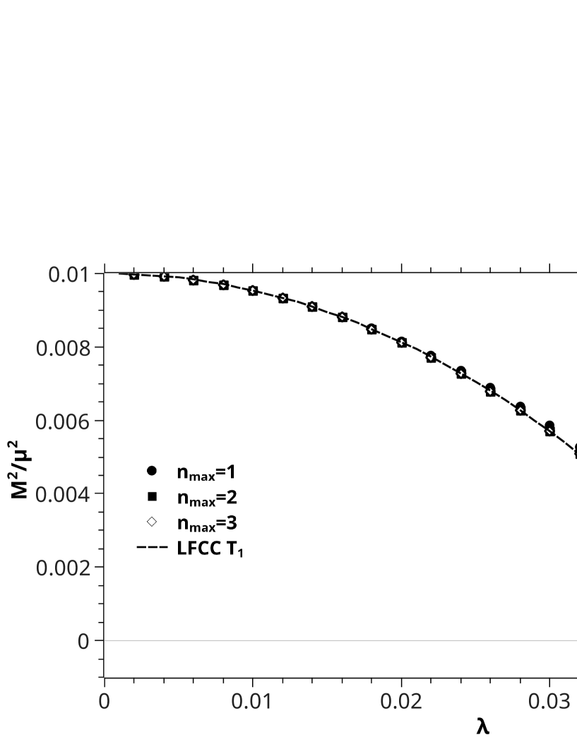
Figure 8: The mass eigenvalue ratio $M^{2}/\mu^{2}$ as a function of the dimensionless coupling $\lambda$ for a series of Fock-space truncations and for the LFCC approximation $T=T_{1}$. The mass ratio of the constituents is $\tilde{m}\equiv m/\mu=0.1$. The basis sets in each Fock sector were limited to orders $N=10$, 14, and 7 for $n_{\rm max}=1$, 2, and 3, respectively. The basis set for the LFCC result has a maximum order of $N_{1}=9$. Addition of the $T_{2}$ operator does not significantly change the LFCC results.

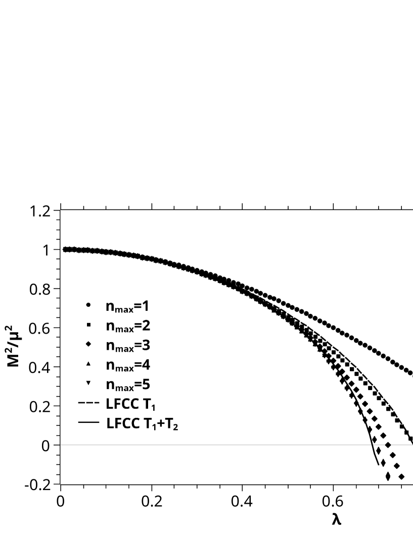
Figure 9: Same as Fig. 8 but for a constituent mass ratio of $\tilde{m}=1$ and with both LFCC approximations $T=T_{1}$ and $T=T_{1}+T_{2}$. The basis sets in each Fock sector were limited to orders $N=2$, 6, 12, 10, and 8 for $n_{\rm max}=1$, 2, 3, 4, and 5, respectively. The basis sets for the LFCC results have maximum orders of $N_{1}=5$ and $N_{2}=5$.

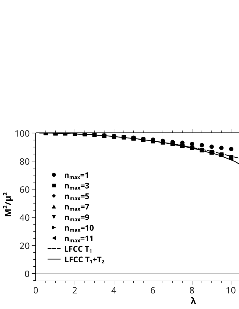
Figure 10: Same as Fig. 9 but for the mass ratio of the constituents is $\tilde{m}=10$. The basis sets in each Fock sector were limited to orders $N=5$, 5, 4, 3, and 3 for $n_{\rm max}=1$, 2, 3, 4, and 5, respectively, and to $N=2$ for all higher Fock sectors. The basis sets for the LFCC results have maximum orders of $N_{1}=5$ and $N_{2}=3$. In this case, the Fock-space expansion has not converged near $M=0$. Also, the nonlinear system solver failed to converge for the LFCC approximation with $\lambda$ beyond 10.6 when $T_{2}$ was included.

From the solutions to the LFCC equations, we compute the mass eigenvalues $M$ and the relative probabilities of the one and two-neutral Fock sectors. The masses are shown in Figs. 8-10, where we plot results for both $T_{1}$ alone and $T_{1}+T_{2}$.

Results for relative probabilities are plotted in Figs. 11-13. These show that as the neutral constituents become lighter, making $\tilde{m}$ larger, the importance of the higher Fock sectors increases dramatically. The LFCC approximation for the one-neutral Fock wave function yields a nearly exact match to the one-neutral relative probability; this is seen in Figs. 11-13, where the solid line representing the LFCC result passes through the points from the converged Fock-state-expansion results for the one-neutral probabilities. We interpret this agreement to mean that the effect of the higher Fock sectors on the one-neutral wave function is well represented by the LFCC approximation to these higher sectors.

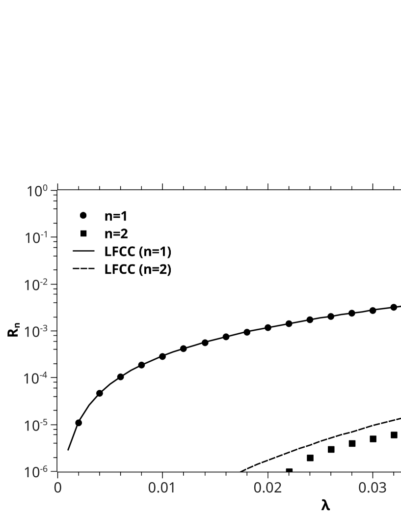
Figure 11: Relative probabilities $R_{n}$ for a sequence of Fock sectors as functions of the dimensionless coupling $\lambda$ for a constituent mass ratio of $\tilde{m}=0.1$. Results for the one and two-neutrals Fock sectors in the LFCC approximation are also included.

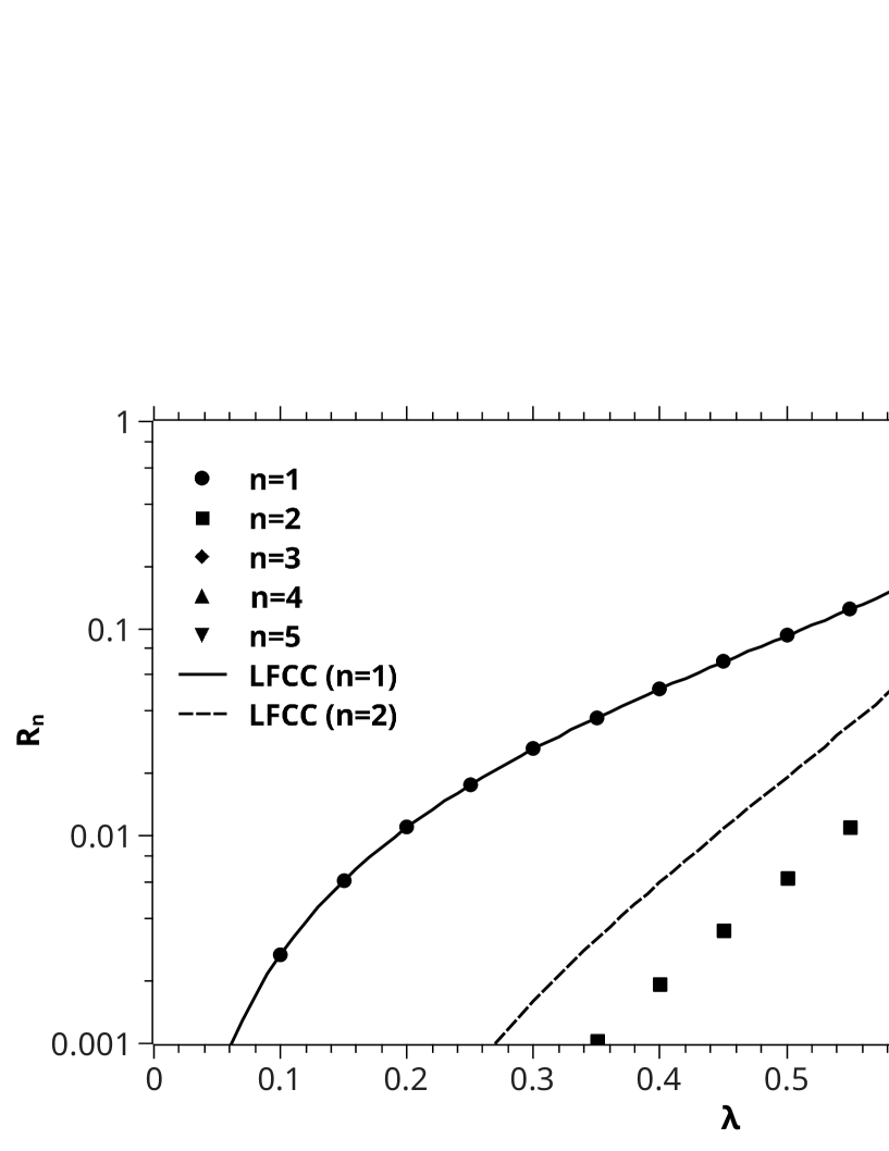
Figure 12: Same as Fig. 11 but for $\tilde{m}=1$.

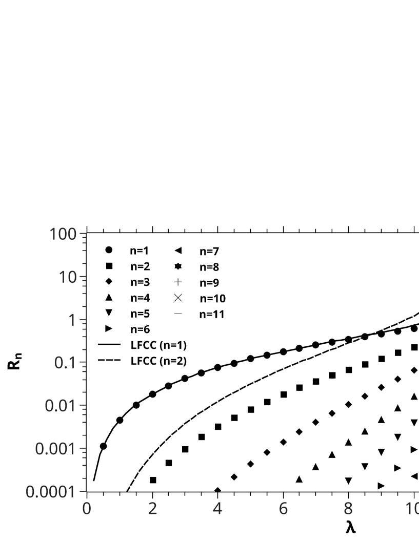
Figure 13: Same as Fig. 11 but for $\tilde{m}=10$.

The results show that the LFCC truncation to $T_{1}+T_{2}$ is sufficient to replicate the converged Fock-state expansion results, with $T_{1}$ alone just as good as a two or three-neutral Fock-sector truncation. Thus the LFCC approximation, using only the two functions $t_{1}(y)$ and $t_{2}(y_{1},y_{2})$ of one and two variables, respectively, is sufficient to represent information that the Fock-space expansion encodes in many more wave functions. In addition, the number of basis functions required to represent the Fock wave functions is significantly greater than the number required for the LFCC functions. Thus, the matrix representation is much smaller for the LFCC approximation, which is ample compensation for its nonlinearity.

The failure of the nonlinear solver to converge for strong coupling in the ultrarelativistic case occurs in the same coupling range where the Fock-state expansion fails to converge. This is near where $M$ tends to zero and may be indicative of the incompleteness of theory. Quenching may have stabilized the spectrum, but the theory is no longer a complete quantum theory. As discussed in the Introduction, a similar lack of solution convergence has been observed in $\phi^{4}$ theory LFCCphi4 .

V Summary

We have shown that the LFCC approximation provides an efficient representation of a massive eigenstate in quenched scalar Yukawa theory. We have also found that the LFCC approximation converges quickly as more terms are added to the $T$ operator. From a numerical standpoint, there is also an efficiency in the basis size required for a matrix representation of the fundamental equations; the LFCC functions are fewer in number than the Fock wave functions, depend on fewer variables, and need fewer basis functions for their accurate representation.

In doing these calculations, we have developed diagrammatic methods for the construction of the LFCC equations. These significantly reduce the effort involved, compared to literally carrying out contractions of creation and annihilation operators in matrix elements of the effective LFCC Hamiltonian. Extension to other theories should be straightforward.

Appendix A Numerical methods

A.1 Fock-state expansion

We solve the coupled system (II) for the Fock-state wave functions $\psi_{n}$ in (13) by first expanding the wave functions in a simple polynomial basis

$$\psi_{n}(y_{1},\ldots,y_{n})=\sqrt{y_{1}\cdots y_{n}(1-\sum_{i}y_{i})}\sum_{mj}^{N}c_{mj}^{(n)}P_{mj}^{(n)}(y_{1},\ldots,y_{n}),$$ (29)

where $m$ is the order of the polynomial $P_{mj}^{(n)}$, $j$ is an index that differentiates distinct polynomials of the same order (which is nontrivial for multivariate polynomials), $N$ is the maximum order included, and the $c_{mi}^{(n)}$ are unknown coefficients to be obtained. The polynomials are chosen to be simple monomials, suitably symmetrized but not orthogonal. They take the form

$$P_{mj}^{(n)}(y_{1},\ldots,y_{n})=y_{1}^{j_{1}}y_{2}^{j_{2}}\ldots y_{n}^{j_{n}}+\cdots,$$ (30)

with $\sum_{i}^{n}j_{i}=m$. The truncation of the basis to the order $N$ is, of course, an approximation necessary for a finite matrix representation; we study convergence with the respect to this truncation, allowing $N$ to be different for each Fock sector.

Projection of the nth equation onto each basis function, $\sqrt{y_{1}\cdots y_{n}(1-\sum_{i}y_{i})}P_{m^{\prime}j^{\prime}}^{(n)}(y_{1},\ldots,y_{n})$, yields a matrix representation of the original coupled system

$$\sum_{mj}\left[T^{(n)}_{m^{\prime}j^{\prime},mj}c_{mj}^{(n)}+V^{(n,n+1)}_{m^{\prime}j^{\prime},mj}c_{mj}^{(n+1)}+V^{(n,n-1)}_{m^{\prime}j^{\prime},mj}c_{mj}^{(n-1)}\right]=\frac{M^{2}}{\mu^{2}}\sum_{mj}S^{(n)}_{m^{\prime}j^{\prime},mj}c_{mj}^{(n)}.$$ (31)

The individual matrices are

$$T^{(n)}_{m^{\prime}j^{\prime},mj}=\int\prod_{i}^{n}dy_{i}\left[\tilde{m}^{2}y_{1}\cdots y_{n}+ny_{2}\cdots y_{n}\right]P_{m^{\prime}j^{\prime}}^{(n)}(y_{1},\ldots,y_{n})P_{mj}^{(n)}(y_{1},\ldots,y_{n}),$$ (32)

$$V^{(n,n+1)}_{m^{\prime}j^{\prime},mj}=\lambda\sqrt{n+1}\int\prod_{i}^{n}dy_{i}\int_{0}^{1-\sum_{i}y_{i}}dx\,y_{1}\cdots y_{n}P_{m^{\prime}j^{\prime}}^{(n)}(y_{1},\ldots,y_{n})P_{mj}^{(n+1)}(y_{1},\ldots,y_{n},x),$$ (33)

$$V^{(n,n-1)}_{m^{\prime}j^{\prime},mj}=\lambda\sqrt{n}\int\prod_{i}^{n}dy_{i}\,y_{1}\cdots y_{n-1}P_{m^{\prime}j^{\prime}}^{(n)}(y_{1},\ldots,y_{n})P_{mj}^{(n-1)}(y_{1},\ldots,y_{n-1}),$$ (34)

and

$$S^{(n)}_{m^{\prime}j^{\prime},mj}=\int\prod_{i}^{n}dy_{i}\,y_{1}\cdots y_{n}(1-\sum_{i}y_{i})P_{m^{\prime}j^{\prime}}^{(n)}(y_{1},\ldots,y_{n})P_{mj}^{(n)}(y_{1},\ldots,y_{n}).$$ (35)

The integrals can be done analytically in terms of the generalized $\beta$ function

$$\int dx_{1}\cdots dx_{n}\,x_{1}^{k_{1}}\cdots x_{n}^{k_{n}}(1-x_{1}-\cdots-x_{n})=\frac{k_{1}!\cdots k_{n}!}{(k_{1}+\cdots+k_{n}+n+2)!}$$ (36)

This allows for efficient calculation of all the integrals, with the different $\beta$-function evaluations done recursively and stored for use.

If the basis functions were orthogonal, $S^{(n)}$ would be diagonal, of course. However, we implicitly orthogonalize the basis by performing a singular-value decomposition $S^{(n)}=U^{(n)}W^{(n)}U^{(n)T}$. The columns of the matrix $U^{(n)}$ are the eigenvectors of $S^{(n)}$, and $W^{(n)}$ is a diagonal matrix of the eigenvalues. The $U$ matrices then define an orthogonal transformation to new vectors of coefficients $\vec{c}^{\,(n)\prime}=(W^{(n)})^{1/2}U^{(n)T}\vec{c}^{\,(n)}$ and new matrices, such as $T^{(n)\prime}=(W^{(n)})^{-1/2}U^{(n)T}T^{(n)}U^{(n)}(W^{(n)})^{-1/2}$. The new matrix problem is no longer of the generalized type, but simply

$$\sum_{mj}\left[T^{(n)\prime}_{m^{\prime}j^{\prime},mj}c_{mj}^{(n)\prime}+V^{(n,n+1)\prime}_{m^{\prime}j^{\prime},mj}c_{mj}^{(n+1)\prime}+V^{(n,n-1)\prime}_{m^{\prime}j^{\prime},mj}c_{mj}^{(n-1)\prime}\right]=\frac{M^{2}}{\mu^{2}}c_{m^{\prime}j^{\prime}}^{(n)\prime}.$$ (37)

The lowest eigenvalue is extracted by standard procedures for symmetric matrices.

The convergence of such a calculation, with respect to the basis size, is illustrated in Fig. 14. Convergence is quite rapid in general; for stronger coupling values, near where $M$ becomes zero, larger basis sizes are needed.

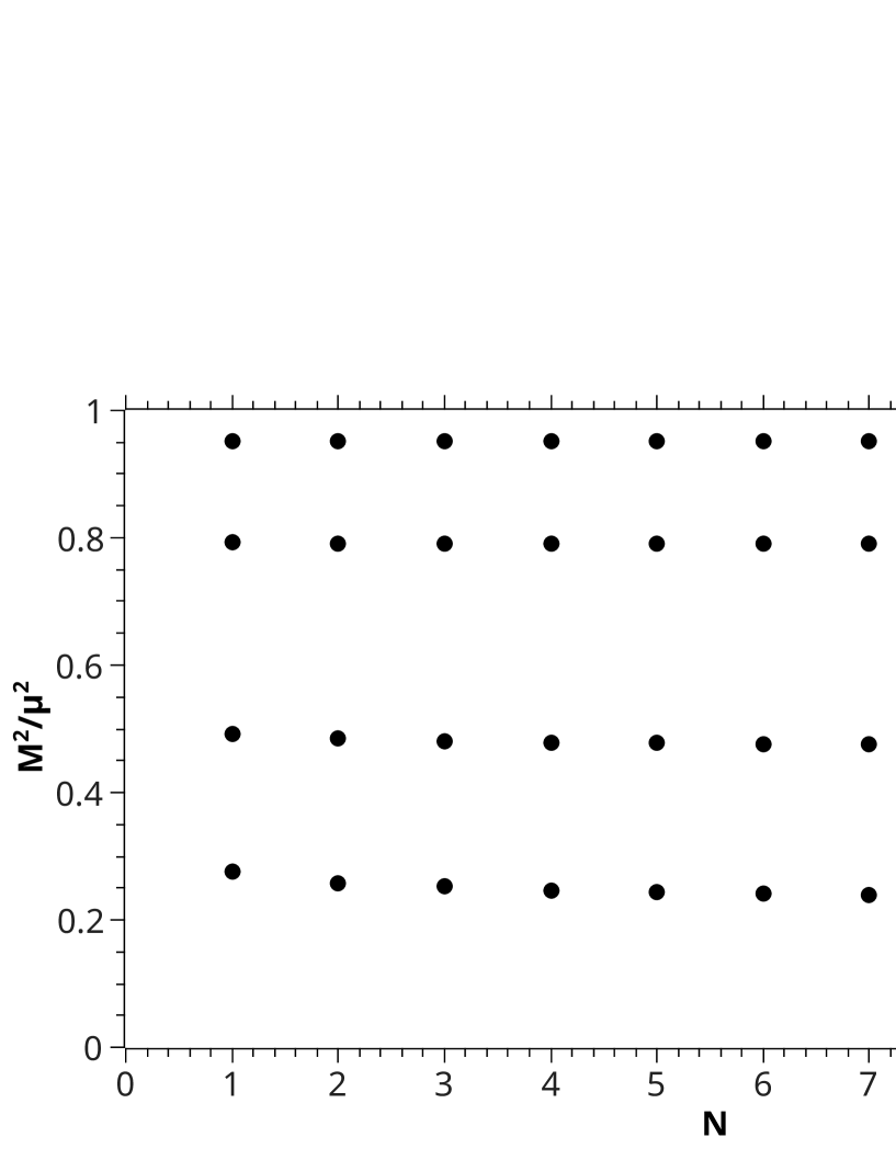
Figure 14: The mass eigenvalue as a function of the basis order $N$ in the top Fock sector of two neutrals for selected coupling strengths $\lambda=0.2$, 0.4, 0.6, and 0.7. The mass values decrease with increasing $\lambda$. The constituent mass ratio $\tilde{m}$ is equal to 1. The maximum polynomial order in the one-neutral sector is 2.

A.2 LFCC approximation

To solve the LFCC equations for $t_{1}$ and $t_{2}$, given in (III) and (III), we expand these functions in the basis set used for the Fock-state wave functions as

$$t_{1}(y)=\sqrt{y(1-y)}\sum_{m}^{N_{1}}a_{m}P_{m}^{(1)}(y),\;\;t_{2}(y_{1},y_{2})=\sqrt{y_{1}y_{2}(1-y_{1}-y_{2})}\sum_{m}^{N_{2}}b_{m}P_{m}^{(2)}(y_{1},y_{2}).$$ (38)

Here the index $m$ represents both the order and implicitly, in the case of two variables, the distinction between linearly independent polynomials of the same order. The equation for $t_{1}$ is projected onto the single-variable basis functions $\sqrt{y(1-y)}P_{m^{\prime}}^{(1)}(y)$, and the equation for $t_{2}$ is projected onto $\sqrt{y_{1}y_{2}(1-y_{1}-y_{2})}P_{m^{\prime}}^{(2)}(y_{1},y_{2})$. The matrix representation of the equation for $t_{1}$ is then

$$0 = (\tilde{m}^{2}+\frac{\lambda}{2}\Delta)A_{m^{\prime}m}^{1}a_{m}-(\tilde{m}^{2}+\lambda\Delta)A_{m^{\prime}m}^{2}a_{m}+B_{m^{\prime}m}a_{m}+\lambda C_{m^{\prime}}+\frac{\lambda}{2}D_{m^{\prime}ml}a_{m}a_{l}+2\lambda F_{m^{\prime}m}b_{m}$$

and that for $t_{2}$ is

$$0 = 2\left[(\tilde{m}^{2}+\frac{\lambda}{2}\Delta)G_{m^{\prime}m}^{1}-(\tilde{m}^{2}+\lambda\Delta)G_{m^{\prime}m}^{2}+G_{m^{\prime}m}^{3}\right]b_{m}$$

$$+\left[(\tilde{m}^{2}+\frac{\lambda}{3}\Delta)H_{m^{\prime}ml}^{1}-2(\tilde{m}^{2}+\frac{\lambda}{2}\Delta)H_{m^{\prime}ml}^{2}+(\tilde{m}^{2}+\lambda\Delta)H_{m^{\prime}ml}^{3}+H_{m^{\prime}ml}^{4}\right]a_{m}a_{l}$$

$$+2\lambda I_{m^{\prime}m}a_{m}+\frac{\lambda}{3}J_{m^{\prime}mkl}a_{m}a_{k}a_{l}+\lambda K_{m^{\prime}ml}b_{m}a_{l},$$

with sums over repeated indices implied,

$$\Delta=\sum_{m}C_{m}a_{m}$$ (41)

and the associated matrices defined by

$$A_{m^{\prime}m}^{1} = \int_{0}^{1}dy\,yP_{m^{\prime}}^{(1)}(y)P_{m}^{(1)}(y),$$ (42)

$$A_{m^{\prime}m}^{2} = \int_{0}^{1}dy\,y(1-y)P_{m^{\prime}}^{(1)}(y)P_{m}^{(1)}(y)$$ (43)

$$B_{m^{\prime}m} = \int_{0}^{1}dy\,(1-y)P_{m^{\prime}}^{(1)}(y)P_{m}^{(1)}(y)$$ (44)

$$C_{m^{\prime}} = \int_{0}^{1}dyP_{m^{\prime}}^{(1)}(y)$$ (45)

$$D_{m^{\prime}ml} = \int_{0}^{1}dy\int_{0}^{1-y}dx\frac{y}{1-x}P_{m^{\prime}}^{(1)}(y)P_{m}^{(1)}(\frac{y}{1-x})P_{l}^{(1)}(x)$$

$$= \int_{0}^{1}dx\int_{0}^{1}dz\,z(1-x)P_{m^{\prime}}^{(1)}(z(1-x))P_{m}^{(1)}(z)P_{l}^{(1)}(x)$$

$$F_{m^{\prime}m} = \int_{0}^{1}dy\int_{0}^{1-y}dx\,yP_{m^{\prime}}^{(1)}(y)P_{m}^{(2)}(y,x)$$ (47)

$$G_{m^{\prime}m}^{1} = \int_{0}^{1}dy_{1}dy_{2}\,y_{1}y_{2}P_{m^{\prime}}^{(2)}(y_{1},y_{2})P_{m}^{(2)}(y_{1},y_{2})$$ (48)

$$G_{m^{\prime}m}^{2} = \int_{0}^{1}dy_{1}dy_{2}\,y_{1}y_{2}(1-y_{1}-y_{2})P_{m^{\prime}}^{(2)}(y_{1},y_{2})P_{m}^{(2)}(y_{1},y_{2})$$ (49)

$$G_{m^{\prime}m}^{3} = 2\int_{0}^{1}dy_{1}dy_{2}\,y_{2}(1-y_{1}-y_{2})P_{m^{\prime}}^{(2)}(y_{1},y_{2})P_{m}^{(2)}(y_{1},y_{2})$$ (50)

$$H_{m^{\prime}ml}^{1} = \int_{0}^{1}dy_{1}dz_{2}\,y_{1}z_{2}(1-y_{1})P_{m^{\prime}}^{(2)}(y_{1},z_{2}(1-y_{1}))P_{m}^{(1)}(y_{1})P_{l}^{(1)}(z_{2})$$ (51)

$$H_{m^{\prime}ml}^{2} = \int_{0}^{1}dy_{1}dz_{2}\,y_{1}z_{2}(1-y_{1})(1-z_{2})P_{m^{\prime}}^{(2)}(y_{1},z_{2}(1-y_{1}))P_{m}^{(1)}(y_{1})P_{l}^{(1)}(z_{2})$$ (52)

$$H_{m^{\prime}ml}^{3} = \int_{0}^{1}dy_{1}dz_{2}\,y_{1}z_{2}(1-y_{1})^{2}(1-z_{2})P_{m^{\prime}}^{(2)}(y_{1},z_{2}(1-y_{1}))P_{m}^{(1)}(y_{1})P_{l}^{(1)}(z_{2})$$ (53)

$$H_{m^{\prime}ml}^{4} = \int_{0}^{1}dy_{1}dz_{2}\,y_{1}(1-y_{1})(1-z_{2})P_{m^{\prime}}^{(2)}(y_{1},z_{2}(1-y_{1}))P_{m}^{(1)}(y_{1})P_{l}^{(1)}(z_{2})$$

$$-\int_{0}^{1}dy_{1}dz_{2}\,z_{2}(1-y_{1})^{2}(1-z_{2})P_{m^{\prime}}^{(2)}(y_{1},z_{2}(1-y_{1}))P_{m}^{(1)}(y_{1})P_{l}^{(1)}(z_{2})$$

$$I_{m^{\prime}m} = \int_{0}^{1}dy_{1}dy_{2}\,y_{1}P_{m^{\prime}}^{(2)}(y_{1},y_{2})P_{m}^{(1)}(y_{1})$$

$$-\int_{0}^{1}dy_{1}dz_{2}\,z_{2}(1-y_{1})(1-z_{2})P_{m^{\prime}}^{(2)}(y_{1},z_{2}(1-y_{1}))P_{m}^{(1)}(z_{2})$$

$$J_{m^{\prime}mkl} = \int_{0}^{1}dy_{1}dz_{1}dz_{2}\left[y_{1}z_{2}(1-y_{1})(1-z_{1})P_{m^{\prime}}^{(2)}(y_{1},z_{2}(1-y_{1})(1-z_{1}))\right.$$

$$-3z_{1}(1-y_{1})z_{2}(1-z_{1}(1-y_{1}))^{2}(1-z_{2})P_{m^{\prime}}^{(2)}(z_{1}(1-y_{1}),z_{2}(1-y_{1})(1-z_{1}))$$

$$\left.+z_{1}(1-y_{1})z_{2}(1-z_{1})(1-y_{1}))P_{m^{\prime}}^{(2)}(z_{1}(1-y_{1}),z_{2}(1-y_{1})(1-z_{1}))\right]$$

$$\rule{36.135pt}{0.0pt}\times P_{m}^{(1)}(z_{2})P_{k}^{(1)}(z_{1})P_{l}^{(1)}(y_{1})$$

$$K_{m^{\prime}ml} = \int_{0}^{1}dy_{1}dz_{1}dz_{2}\left[z_{1}z_{2}(1-y_{1})^{2}(1-z_{1})^{2}P_{m^{\prime}}^{(2)}(z_{1}(1-y_{1}),z_{2}(1-y_{1})(1-z_{1}))\right.$$

$$\rule{216.81pt}{0.0pt}\times P_{m}^{(2)}(z_{1},z_{2}(1-z_{1}))P_{l}^{(1)}(y_{1})$$

$$+2y_{1}z_{2}(1-y_{1})(1-z_{2})P_{m^{\prime}}^{(2)}(y_{1},z_{2}(1-y_{1}))P_{m}^{(2)}(z_{1}(1-z_{2}),z_{2}))P_{l}^{(1)}(y_{1})$$

$$-4y_{1}z_{2}(1-y_{1})^{2}(1-z_{2})P_{m^{\prime}}^{(2)}(y_{1},z_{2}(1-y_{1}))P_{m}^{(2)}(z_{1}(1-y_{1}),y_{1}))P_{l}^{(1)}(z_{2})$$

$$\left.+2y_{1}z_{2}(1-y_{1})^{2}(1-z_{1})P_{m^{\prime}}^{(2)}(y_{1},z_{2}(1-y_{1})(1-z_{1}))P_{m}^{(2)}(y_{1},z_{1}(1-y_{1}))P_{l}^{(1)}(z_{2})\right].$$

For the $D$ matrix, a change of variables has been shown explicitly; similar rescalings are done for many of the other matrices. These rescalings arrange for the arguments of the polynomials to be polynomials and for all integration ranges to be from 0 to 1. The integrals are then linear combinations of simple integrals of monomials.

The nonlinear matrix equations obtained in this way are then solved by a modification of the Powell hybrid method Powell as implemented in the general nonlinear equation solver ‘hybrj’ of the MINPACK set of subroutines minpack . The method is recursive; the initial guess for the unknown coefficients is taken to be zero for the lowest coupling strength and, as an increasing series of coupling strengths is considered, the next initial guess is the solution for the previous coupling strength.

For the case where only $T_{1}$ is included and we solve only (III) for $t_{1}$ with $t_{2}=0$, convergence with respect to basis size is very rapid when $\tilde{m}=1$. The results for $N_{1}=1$ and $N_{1}=2$ are indistinguishable on a graph. For the full solution, with both $T_{1}$ and $T_{2}$ included, the dependence on $N_{2}$, the maximum order for the $t_{2}$ basis, is shown in Fig. 15. Convergence is again quite rapid, except for stronger coupling where $M^{2}$ approaches zero. For smaller and larger values of $\tilde{m}$, convergence is slower for $t_{1}$, requiring $N_{1}=9$ for $\tilde{m}=0.1$ and $N_{1}=5$ for $\tilde{m}=10$. Convergence for $t_{2}$ is quicker, using $N_{2}=3$, except for strong coupling in the case of $\tilde{m}=10$ where the nonlinear equation solver was unable to converge to a solution.

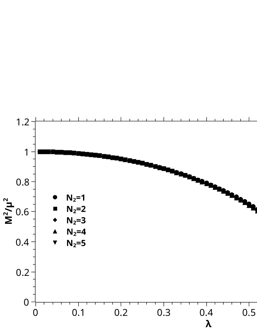
Figure 15: LFCC results for the mass eigenvalue ratio $M^{2}/\mu^{2}$ as a function of the dimensionless coupling $\lambda$ for a range of basis sizes for $t_{2}$. The basis set was limited to maximum order of $N_{2}=1$ through 5, with the $t_{1}$ basis size set at maximum order $N_{1}=2$. The mass ratio of the constituents is $\tilde{m}\equiv m/\mu=1$.

Appendix B Rules for diagrams

Although the LFCC equations for the $t$ functions can be constructed by carrying out the contractions of creation and annihilation operators, the construction can be simplified by use of a set of rules for operator diagrams that depict the structure of the contractions. The rules are as follows:

1. Represent the terms of ${\cal P}^{-}$ by crosses for the charged and neutral mass terms and simple vertices for neutral creation and annihilation, as shown in Fig. 16.

2. Represent $T_{1}$ and $T_{2}$ by the vertices shown in Fig. 17.

3. For each Fock-sector projection, draw all possible diagrams connecting the valence state to that Fock sector. The connections between vertices and/or crosses represent contractions. Each diagram must include a term from ${\cal P}^{-}$ once and only once and may include as many $T_{1}$ and/or $T_{2}$ vertices as needed, to the left and right of the ${\cal P}^{-}$ insertion, to reach the chosen sector.

4. In each diagram, label each line with a momentum fraction, starting from 1 for the line acting on the charge-one valence state on the right and ending with $y_{1}$ through $y_{n}$ for the $n$ neutrals in the projected sector on the left; conserve momentum at each vertex.

5. Construct the expression corresponding to the diagram from the individual vertices and crosses, and integrate over any loop momentum fractions, with the upper limit set by the fractions entering and leaving the loop.

6. For each product of $m$ $T_{1}$ and $T_{2}$ vertices to the left, include a factor of $(-1)^{m}/m!$ and for each to right, a factor of $1/m!$; these come from the expansion of the exponential $e^{\pm(T_{1}+T_{2})}$.

7. Symmetrize with respect to permutations of $y_{1},\ldots,y_{n}$ and with respect to the neutral lines from $T_{2}$ vertices.

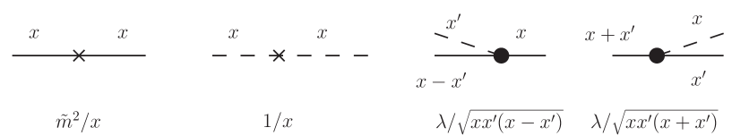
Figure 16: Diagrammatic representation of the terms in ${\cal P}^{-}$ and their corresponding expressions. Solid lines represent the charged scalar and dashed, the neutral. A cross designates a mass term. The diagrams represent operators acting to the right; for example, the last diagram corresponds to the annihilation of a neutral.

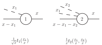
Figure 17: Diagrammatic representation of the $T_{1}$ and $T_{2}$ operators, and their corresponding expressions, acting to the right and creating one or two neutrals, respectively, by first annihilating a charged scalar with momentum fraction $x$.

As an almost trivial example, the diagrams contributing to the terms on the right of the valence equation (20) are shown in Fig. 1. A less trivial example is the set of diagrams for the one-neutral projection, shown in Fig. 2. Except for the $\frac{1}{2}{\cal P}^{-}_{\rm int}T_{1}^{2}$ term in (22), there is only one diagram for each term in $\overline{{\cal P}^{-}}$; for $\frac{1}{2}{\cal P}^{-}_{\rm int}T_{1}^{2}$ there are two. The rules then yield (III).

References

- (1) C. Gattringer and C.B. Lang, Quantum Chromodynamics on the Lattice (Springer, Berlin, 2010); H. Rothe, Lattice Gauge Theories: An Introduction, 4e (World Scientific, Singapore, 2012).
- (2) P.A.M. Dirac, Rev. Mod. Phys. 21, 392 (1949).
- (3) For reviews of light-cone quantization, see M. Burkardt, Adv. Nucl. Phys. 23, 1 (2002); S.J. Brodsky, H.-C. Pauli, and S.S. Pinsky, Phys. Rep. 301, 299 (1998); J.R. Hiller, Prog. Part. Nucl. Phys. 90, 75 (2016).
- (4) H.-C. Pauli and S.J. Brodsky, Phys. Rev. D 32, 1993 (1985); 32, 2001 (1985).
- (5) J.P. Vary, H. Honkanen, J. Li, P. Maris , S.J. Brodsky, A. Harindranath, G.F. de Teramond, P. Sternberg, E.G. Ng, and C. Yang Phys. Rev. C 81, 035205 (2010).
- (6) R.J. Perry, A. Harindranath, and K.G. Wilson, Phys. Rev. Lett. 65, 2959 (1990); R.J. Perry and A. Harindranath, Phys. Rev. D 43, 4051 (1991).
- (7) J.R. Hiller and S.J. Brodsky, Phys. Rev. D 59, 016006 (1998).
- (8) V.A. Karmanov, J.-F. Mathiot, and A.V. Smirnov, Phys. Rev. D 77, 085028 (2008); Phys. Rev. D 82, 056010 (2010).
- (9) S.S. Chabysheva and J.R. Hiller, Ann. Phys. 325, 2435 (2010).
- (10) S.S. Chabysheva and J.R. Hiller, Phys. Lett. B 711, 417 (2012).
- (11) R.J Bartlett and M. Musial, Rev. Mod. Phys. 79, 291 (2007).
- (12) B. Elliott, S.S. Chabysheva, and J.R. Hiller, Phys. Rev. D 90, 056003 (2014).
- (13) G.C. Wick, Phys. Rev. 96, 1124 (1954); R.E. Cutkosky, Phys. Rev. 96, 1135 (1954); E. Zur Linden and H. Mitter, Nuovo Cim. B 61, 389 (1969); D. Bernard, Th. Cousin, V.A. Karmanov, and J.-F. Mathiot, Phys. Rev. D 65, 025016 (2001); Y. Li, V.A. Karmanov, P. Maris, and J.P. Vary, Phys. Lett. B 748, 278 (2015).
- (14) G. Baym, Phys. Rev. 117, 886 (1960); F. Gross, C. Savkli, and J. Tjon, Phys. Rev. D 64, 076008 (2001).
- (15) M. Burkardt, S.S. Chabysheva, and J.R. Hiller, Phys. Rev. D 94, 065006 (2016); S.S. Chabysheva and J.R. Hiller, Phys. Rev. D 95, 096016 (2017).
- (16) J. Collins, “The non-triviality of the vacuum in light-front quantization: An elementary treatment,” arXiv:1801.03960 [hep-ph].
- (17) L. Martinovic̆ and A. Dorokhov, “Vacuum loops in light-front field theory,” arXiv:1812.02336 [hep-th].
- (18) S.S. Chabysheva and J.R. Hiller, “Transitioning from equal-time to light-front quantization in theory,” arXiv:1811.01685 [hep-th].
- (19) A.L. Fitzpatrick, J. Kaplan, E. Katz, L.G. Vitale, and M.T. Walters, JHEP 1808, 120 (2018); A.L. Fitzpatrick, E. Katz, and M.T. Walters, “Nonperturbative matching between equal-time and light-cone quantization,” arXiv:1812.08177 [hep-th].
- (20) S. Rychkov and L.G. Vitale, Phys. Rev. D 91, 085011 (2015); Phys. Rev. D 93, 065014 (2016).
- (21) D. Binosi and L. Theußl, Comp. Phys. Comm. 161, 76 (2004).
- (22) M.J.D. Powell, Comp. J. 7, 155 (1964); in Numerical methods for nonlinear algebraic equations, P. Rabinowitz, ed., (Gordon and Breach, New York, 1970), 87-114.
- (23) J.J. Moré, B.S. Garbow, and K.E. Hillstrom, User Guide for MINPACK-1, Argonne National Laboratory Report ANL-80-74, Argonne, IL, 1980.