Hyper-Scalable JSQ with Sparse Feedback

Abstract.

Load balancing algorithms play a vital role in enhancing performance in data centers and cloud networks. Due to the massive size of these systems, scalability challenges, and especially the communication overhead associated with load balancing mechanisms, have emerged as major concerns. Motivated by these issues, we introduce and analyze a novel class of load balancing schemes where the various servers provide occasional queue updates to guide the load assignment.

We show that the proposed schemes strongly outperform JSQ($d$) strategies with comparable communication overhead per job, and can achieve a vanishing waiting time in the many-server limit with just one message per job, just like the popular JIQ scheme. The proposed schemes are particularly geared however towards the sparse feedback regime with less than one message per job, where they outperform corresponding sparsified JIQ versions.

We investigate fluid limits for synchronous updates as well as asynchronous exponential update intervals. The fixed point of the fluid limit is identified in the latter case, and used to derive the queue length distribution. We also demonstrate that in the ultra-low feedback regime the mean stationary waiting time tends to a constant in the synchronous case, but grows without bound in the asynchronous case.

1. Introduction

Background and motivation. We introduce and analyze hyper-scalable load balancing algorithms that only involve minimal communication overhead and yet deliver excellent performance. Load balancing algorithms play a key role in efficiently distributing jobs (e.g. compute tasks, database look-ups, file transfers) among servers in cloud networks and data centers (Gandhi et al., 2014; Maguluri et al., 2012; Patel et al., 2013). Well-designed load balancing schemes provide an effective mechanism for improving performance metrics in terms of response times while achieving high resource utilization levels. Besides these typical performance criteria, communication overhead and implementation complexity have emerged as equally crucial attributes, due to the immense size of cloud networks and data centers. These scalability challenges have fueled a strong interest in the design of load balancing algorithms that provide robust performance while only requiring low overhead.

We focus on a basic scenario of $N$ parallel identical servers, exponentially distributed service requirements, and a service discipline at each server that is oblivious to the actual service requirements (e.g. FCFS). In this canonical case, the Join-the-Shortest-Queue (JSQ) policy has strong stochastic optimality properties, and in particular minimizes the overall mean delay among the class of non-anticipating load balancing policies that do not have any advance knowledge of the service requirements (Ephremides et al., 1980; Winston, 1977).

In order to implement the JSQ policy, a dispatcher requires instantaneous knowledge of the queue lengths at all the servers, which may give rise to a substantial communication burden, and not be scalable in scenarios with large numbers of servers. The latter issue has motivated consideration of so-called JSQ($d$) strategies, where the dispatcher assigns incoming jobs to a server with the shortest queue among $d$ servers selected uniformly at random. This involves an exchange of $2d$ messages per job (assuming $d\geq 2$), and thus greatly reduces the communication overhead compared to the JSQ policy when the number of servers $N$ is large. At the same time, results in Mitzenmacher (Mitzenmacher, 2001) and Vvedenskaya et al. (Vvedenskaya et al., 1996) indicate that even a value as small as $d=2$ yields significant performance improvements as $N\to\infty$ compared to a purely random assignment scheme ($d=1$). This is commonly referred to as the “power-of-two” effect.

Although JSQ($d$) strategies provide notably better waiting-time performance than purely random assignment, they lack the ability of the conventional JSQ policy to drive the waiting time to zero in the many-server limit. Moreover, while JSQ($d$) strategies notably reduce the amount of communication overhead compared to the full JSQ policy, the two-way delay incurred in obtaining queue length information still directly adds to the waiting time of each job. The latter achilles heel of ‘push-based’ strategies is eliminated in ‘pull-based’ strategies where servers pro-actively provide queue length information to the dispatcher. A particularly popular pull-based strategy is the so-called Join-the-Idle-Queue (JIQ) scheme (Badonnel and Burgess, 2008; Lu et al., 2011). Servers advertise their availability to the dispatcher whenever they become idle, which involves no more than one message per job to send a job to an available idle server. This pull-based strategy has the ability of the full JSQ policy to achieve a zero waiting time in the many-server limit (Stolyar, 2015). A pull-based implementation for the JSQ policy exists but it leads to more frequent communication requirements or larger communication messages.

The superiority of the JIQ scheme over JSQ($d$) strategies in terms of performance and communication overhead is owed to the state information stored at the dispatcher. Results in (Gamarnik et al., 2016) imply that a vanishing waiting time can only be achieved with finite communication overhead per job when allowing memory usage at the dispatcher, and further suggest that one message per job is a minimal requirement in a certain sense. However, even just one message per job may still be prohibitive, especially when jobs do not involve big computational tasks, but small data packets which require little processing, e.g. in IoT cloud environments. In such situations the sheer message exchange in providing queue length information may be disproportionate to the actual amount of processing required.

Hyper-scalable algorithms. Motivated by the above issues, we propose and examine a novel class of load balancing schemes which also leverage memory at the dispatcher, but allow the communication overhead to be seamlessly adapted and reduced below that of the JIQ scheme. The basic scheme is as follows:

Algorithm 1 (Basic hyper-scalable scheme).

The dispatcher forwards incoming jobs to the server with the lowest queue estimate. The dispatcher maintains an estimate for every server and increments these estimates for every job that is assigned. Status updates of servers occur at rate $\delta$ per server, and update the estimate that the dispatcher has at its disposal to the actual queue length.

Several aspects of Algorithm 1 are flexible (regarding the implementation and the status updates) and four different schemes that obey the rules of Algorithm 1 will be introduced. There are many more schemes that could be of interest, for example a scheme where the queue estimate is not an upper-bound but mimics the expected value of the queue length. While natural, these schemes are beyond the scope of the current paper.

When the update frequency per server is $\delta$ and $\lambda<1$ denotes the arrival rate per server, the number of messages per job is $\delta/\lambda$, which can be easily tuned by varying the value of $\delta$. Since all queue lengths are updated (on average) once every $1/\delta$ time units, this gives $\delta N$ queue-updates per time unit. Note that this algorithm can be modeled as a strictly push-based scheme (where the dispatcher requests the queue lengths of the servers), as well as a strictly pull-based scheme (where each server sends its queue length to the dispatcher, using an internal clock).

The JSQ($d$) scheme, when implemented in a push-based manner, requires $2d$ message exchanges per job, which amounts to $2\lambda dN$ messages per time unit and is not scalable. However, when servers actively update their queue lengths to the dispatcher in the JSQ scheme or their idleness in the pull-based JIQ scheme, one needs less communication. In this case, any departing job needs to trigger the server to send an update to the dispatcher. This pull-based implementation requires one message of communication per job or $\lambda N$ per time unit. When queue lengths are large, not even all departing jobs need to trigger the server to send an update for the JIQ policy, which reduces the communication per job slightly. We thus conclude that the tunable communication overhead of $\delta/\lambda$ per job (doubled when implemented in a push-based manner) of Algorithm 1 is comparable with pull-based JSQ, JIQ and JSQ($d$). Moreover, Algorithm 1 becomes more scalable for small values of $\delta$, especially in the $\delta<\lambda$-regime. Here an important reference point is that the pull-based JIQ scheme has at most one update per job. By hyper-scalable schemes we mean schemes that can be implemented with $\delta\leq 1$, and preferably with $\delta\ll 1$.

We introduce four hyper-scalable schemes that obey the rules of Algorithm 1 but differ in when the status-updates are sent. When the updates sent by the servers to the dispatcher are synchronized, we denote the scheme by $\text{SUJSQ}(\delta)$, Synchronized-Updates Join-the-Shortest-Queue. Similarly we introduce $\text{AUJSQ}(\delta)$ (Asynchronized-Updates Join-the-Shortest-Queue), which is used when the updates are asynchronous. We then add an exp-tag whenever the time between two updates is exponentially distributed (with parameter $\delta$ and mean $1/\delta$) and a det-tag when the time between the updates is constant ($1/\delta$). This gives rise to four schemes; $\text{SUJSQ}^{\textup{det}}(\delta)$ , $\text{SUJSQ}^{\textup{exp}}(\delta)$, $\text{AUJSQ}^{\textup{det}}(\delta)$ and $\text{AUJSQ}^{\textup{exp}}(\delta)$.

We show that the four schemes can achieve a vanishing waiting time in the many-server limit with just one message per job, just like JIQ. The proposed schemes are particularly geared however towards the sparse feedback regime with less than message per job, where they outperform corresponding sparsified JIQ versions. With fluid limits we demonstrate that in the ultra-low feedback regime the mean stationary waiting time tends to a constant in the synchronous case, but grows without bound in the asynchronous case. A more detailed overview of our key finding is presented in the next section.

Discussion of additional related work. As mentioned above, Mitzenmacher (Mitzenmacher, 2001) and Vvedenskaya et al. (Vvedenskaya et al., 1996) established mean-field limit results for JSQ($d$) strategies. These results indicate that for any subcritical arrival rate $\lambda<1$, the tail of the queue length distribution at each individual server exhibits super-exponential decay, and thus falls off far more rapidly than the geometric decay in case of purely random assignment. Similar power-of-$d$ effects have been demonstrated for heterogeneous servers, non-exponential service requirements and loss systems (Bramson et al., 2010, 2012; Mukhopadhyay et al., 2016, 2015; Mukhopadhyay and Mazumdar, 2014; Xie et al., 2015). For no single value of $d$, however, a JSQ($d$) strategy can rival the JIQ scheme, which simultaneously achieves low communication overhead and asymptotically optimal performance by leveraging memory at the dispatcher (Gamarnik et al., 2016; Stolyar, 2015). The only exception arises for batches of jobs when the value of $d$ and the batch size grow suitably large, as can be deduced from results in (Ying et al., 2015), but we do not leverage batches in the current paper. As we will show, the hyper-scalable schemes proposed in the present paper are like the JIQ scheme superior to JSQ$(d$) strategies, and also beat corresponding sparsified JIQ versions in the regime $\delta<1$, which is particularly relevant from a scalability standpoint.

Many popular schemes have also been analyzed in the Halfin-Whitt heavy-traffic regime (Mukherjee et al., 2016) and in the non-degenerate slowdown regime (Gupta and Walton, 2019), in which the JIQ scheme is not necessarily optimal.

The use of memory in load balancing has been studied in (Alon et al., 2010; Mitzenmacher et al., 2002) but mostly in a ‘balls-and-bins’ context as opposed to the queueing scenario that we consider. The work in (Mitzenmacher, 2000) considers a similar setup as ours, and examines how much load balancing degrades when old information is used.

In contrast, our focus is on improving the performance by using non-recent information, similarly to (Anselmi and Dufour, 2018). A general framework for deriving fluid limits in the presence of memory is described in (Luczak and Norris, 2013), but assumes that the length of only one queue is kept in memory, while we allow for all queue lengths to be tracked.

Organization of the paper. In Section 2 we discuss our key findings and contributions for the hyper-scalable schemes, obtained through fluid-limit analysis and extensive simulations. In Section 3 we introduce some useful notation and preliminaries, before we turn to a comprehensive analysis of the synchronous and asynchronous cases through the lens of fluid limits in Sections 4 and 5, respectively. In Section 6 we conclude with some summarizing remarks and topics for further research.

2. Key findings and contributions

The precise model we consider consists of $N$ parallel identical servers and one dispatcher. Jobs arrive at the dispatcher as a Poisson process of rate $\lambda N$, where $\lambda$ denotes the job arrival rate per server. Every job is dispatched to one of the servers, after which it joins the queue of the server if the server is busy, or will start its service when the server is idle. The job processing requirements are independent and exponentially distributed with unit mean at each of the servers. We consider several load balancing algorithms for the dispatching of jobs to servers, including the hyper-scalable schemes $\text{SUJSQ}^{\textup{det}}(\delta)$, $\text{SUJSQ}^{\textup{exp}}(\delta)$, $\text{AUJSQ}^{\textup{det}}(\delta)$ and $\text{AUJSQ}^{\textup{exp}}(\delta)$ described in the introduction. In the simulation experiments we will also briefly consider $\text{SUJSQ}^{\textup{det,idle}}(\delta)$, which is similar to $\text{SUJSQ}^{\textup{det}}(\delta)$, except that only idle servers send notifications. We now present the results from simulation studies and the fluid-limit and fixed-point analysis in Sections 4 and 5.

2.1. Large-system performance

In order to explore the performance of the hyper-scalable algorithms in the many-server limit $N\to\infty$, we investigate fluid limits. We analyze their behavior and fixed points, and use these to derive results for the system in stationarity as function of the update frequency $\delta$.

Asymptotically optimal feedback regime. Using fluid-limit analysis, we prove that the proposed schemes can achieve a vanishing waiting time in the many-server limit when the update frequency $\delta$ exceeds $\lambda/(1-\lambda)$. In case servers only report zero queue lengths and suppress updates for non-zero queues, the update frequency required for a vanishing waiting time can in fact be lowered to just $\lambda$, matching the one message per job involved in the JIQ scheme.

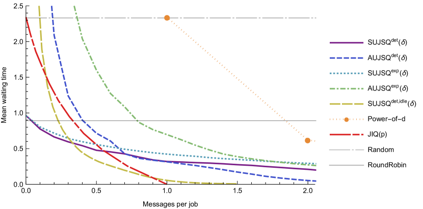
Figure 1. Mean waiting times for different schemes (with various parameters) for $\lambda=0.7$ and $N=200$ obtained via a discrete-event simulation. For each of the schemes, the parameter $\delta$, $d$ or $p$ is varied and the communication in terms of messages per job and the waiting times of jobs are tracked in the simulation.

Sparse feedback regime. Figure 1 displays results from extensive simulations and shows the mean waiting time as function of the number of messages per job. This number is proportional to the update frequency $\delta$, and equals $\delta/\lambda$ for the four hyper-scalable schemes. We also show results for JIQ$(p)$, a sparsified version of JIQ, where a token is sent to the dispatcher with probability $p$ whenever a server becomes idle. Random refers to the scheme where every job is assigned to a server selected uniformly at random, and Round-Robin assigns the $i$-th arriving job to server $1+i\mod N$.

For the sparse feedback regime when $\delta<0.5$ we see that the schemes $\text{SUJSQ}^{\textup{det}}(\delta)$ and $\text{SUJSQ}^{\textup{exp}}(\delta)$ outperform JIQ$(p)$. Also observe that $\text{SUJSQ}^{\textup{det,idle}}(\delta)$, the scheme in which only idle servers send reports, achieves a near-zero waiting time with just one message per job, just like the JIQ scheme, and outperforms JIQ($p$) across most of the relevant domain $\delta<0.5$. However, as $\delta\downarrow 0$ the waiting time grows without bound, since estimates will grow large due to lack of updates, which causes servers that are reported idle in the latest update to receive many jobs in succession.

Ultra-low feedback regime. We examine the performance in the ultra-low feedback regime where the update frequency $\delta$ goes to zero, and in particular establish a somewhat counter-intuitive dichotomy. When all status-updates occur synchronously, the behavior of each of the individual queues approaches that of a single-server queue with a near-deterministic arrival process and exponential service times, with the mean stationary waiting time tending to a finite constant. In contrast, for asynchronous updates, the individual queues experience saw-tooth behavior with oscillations and waiting times that grow without bound.

2.2. Synchronize or not?

In case of synchronized updates, the dispatcher will update the queue lengths of the servers simultaneously. Thus, just after an update moment, the dispatcher has a perfect view of the status of all servers and it will dispatch jobs optimally. After a while, the estimates will start to deviate from the actual queue lengths, so that the scheme no longer makes (close to) optimal decisions. With asynchronous updates servers send updates at independent times, which means that some of the estimates may be very accurate, while others may differ significantly from the actual queue lengths.

Round-Robin resemblance. We find that both $\text{SUJSQ}^{\textup{det}}(\delta)$ and $\text{SUJSQ}^{\textup{exp}}(\delta)$ resemble Round-Robin as the update frequency $\delta$ approaches zero, and are the clear winners in the ultra-low feedback regime, which is crucial from a scalability perspective (see Figure 1). To understand the resemblance with Round-Robin, notice that the initial queue lengths after an update will be small compared to the number of arrivals until the next update. Thus soon after the update the dispatcher will essentially start forwarding jobs in a (probabilistic) Round-Robin manner. Specifically, most servers will have equal queue estimates at certain points in time, and they will each receive one job every $\lambda$ time units, but in a random order. This pattern repeats itself and resembles Round-Robin, where the difference of received jobs among servers can be at most one.

Dichotomy. In Figure 1 we also see that while $\text{AUJSQ}^{\textup{det}}(\delta)$ outperforms the synchronous variants for large values of the update frequency $\delta$, it produces a mean waiting time that grows without bound as $\delta$ approaches zero. The latter issue also occurs for $\text{AUJSQ}^{\textup{exp}}(\delta)$ and render the asynchronous versions far inferior in the ultra-low feedback regime compared to both synchronous variants. To understand this remarkable dichotomy, notice that queue estimates must inevitably grow to increasingly large values of the order $\lambda/\delta$ and significantly diverge from the true queue lengths as the update frequency becomes small, both in the synchronous and asynchronous versions. However, in the synchronous variants the queue estimates will all be lowered and updated to the true queue lengths simultaneously, prompting the dispatcher to evenly distribute incoming jobs over time. In contrast, in the asynchronous versions, a server will be the only one with a low queue estimate right after an update, and almost immediately be assigned a huge pile of jobs to bring its queue estimate at par, resulting in oscillatory effects. This somewhat counter-intuitive dichotomy reveals that the synchronous variants behave benignly in the presence of outdated information, while the asynchronous versions are adversely impacted.

3. Notation and preliminaries

In this section we introduce some useful notation and preliminaries in preparation for the fluid-limit analysis in Sections 4 and 5. Recall that all the servers are identical and the dispatcher only distinguishes among servers based on their queue estimates and does not take their identities into account when forwarding jobs. Hence we do not need to keep track of the state of each individual server, but only count the number of servers that reside in a particular state. Specifically, we will denote by $Y_{i,j}(t)$ the number of servers with queue length $i$ (including a possible job being served) and queue estimate $j\geq i$ at the dispatcher at time $t$. Further denote by $V_{i}=\sum_{l=i}^{\infty}Y_{il}$ and $W_{j}=\sum_{k=0}^{j}Y_{kj}$ the total number of servers with queue length $i$ and queue estimate $j$, respectively, when the system is in state $Y$.

In order to analyze fluid limits in a regime where the number of servers $N$ grows large, we will consider a sequence of systems indexed by $N$, and attach a superscript $N$ to the associated state variables. We specifically introduce the fluid-scaled state variables $y_{i,j}^{N}(t)=Y_{i,j}^{N}(t)/N$, representing the fraction of servers in the $N$-th system with true queue length $i$ and queue estimate $j\geq i$ at the dispatcher at time $t$, and assume that the sequence of initial states is such that $y^{N}(0)\to y^{\infty}$. Any (weak) limit $\{y(t)\}_{t\geq 0}$ of the sequence $(\{y^{N}(t)\}_{t\geq 0})_{N\geq 1}$ as $N\to\infty$ will be called a fluid limit. Fluid limits do not only yield tractability, but also provide a relevant tool to investigate communication overhead and scalability issues which are inherently tied to scenarios with massive numbers of servers.

Let $m(Y)=\min\{j:W_{j}>0\}$ be the minimum queue estimate among all servers when the system is in state $Y$. When a job arrives and the system is in state $Y$, it is dispatched to one of the $W_{m(Y)}$ servers with queue estimate $m(Y)$ selected uniformly at random, so it joins a server with queue length $i\leq m(Y)$ with probability $Y_{i,m(Y)}/W_{m(Y)}$. Because of the Poisson arrival process, transitions from a state $Y$ to a state $Y^{\prime}$ with $Y_{i,j}^{\prime}=Y_{i,j}-1$ and $Y_{i+1,j+1}^{\prime}=Y_{i+1,j+1}+1$ thus occur at rate $\lambda Np_{i,j}(Y)$, with $p_{i,j}(Y)={\mathds{1}}{\left\{{\displaystyle j=m(Y)}\right\}}Y_{i,j}/W_{j}$, $i=0,\dots,j$. Due to the unit-exponential processing requirements, transitions from a state $Y$ to a state $Y^{\prime}$ with $Y_{i,j}^{\prime}=Y_{i,j}-1$ and $Y_{i-1,j}^{\prime}=Y_{i-1,j}+1$ occur at rate $Y_{i,j}$, $i=1,\dots,j$. For notational compactness, we further omit the dependence of $Y$ for $m(Y)$, $p_{i,j}(Y)$ and $q_{i,j}(Y)$ and instead write $m(t)$, $p_{i,j}(t)$ and $q_{i,j}(t)$ as they only depend on $t$ though $y(t)$.

In order to specify the transitions due to the updates, we need to distinguish between the synchronous and the asynchronous case.

Synchronous updates

Whenever a synchronous update occurs and the system is in state $Y$, a transition occurs to state $Y^{\prime}$ with $Y_{ii}^{\prime}=V_{i}$ and $Y_{ij}^{\prime}=0$ for $i=0,\dots,j-1$. Note that these transitions only occur in a Markovian fashion when the update intervals are exponentially distributed. When the update intervals are non-exponentially distributed, $\{Y(t)\}_{t\geq 0}$ is not a Markov process, but the evolution between successive updates is still Markovian.

Asynchronous updates

When the system is in state $Y$ and a server with queue length $i$ and queue estimate $j>i$ sends an update to the dispatcher, a transition occurs to a state $Y^{\prime}$ with $Y^{\prime}_{i,j}=Y_{i,j}-1$ and $Y_{i,i}^{\prime}=Y_{i,i}+1$. Note that these transitions only occur in a Markovian fashion when the update intervals are exponentially distributed. When the update intervals are non-exponentially distributed, $\{Y(t)\}_{t\geq 0}$ is not a Markov process, and in order to obtain a Markovian state description, the state variables $Y_{ij}$ would in fact need to be augmented with continuous variables keeping track of the most recent update moments for the various servers.

4. Synchronous updates

In this section we examine the fluid limit for synchronous updates. In Subsection 4.1 we provide a description of the fluid-limit trajectory, along with an intuitive interpretation, numerical illustration and comparison with simulation. In Subsection 4.2 the fluid-limit analysis will be used to derive a finite upper bound for the queue length on fluid scale for any given update frequency $\delta>0$ (Proposition 4.5) and to show that in the long term queueing vanishes on fluid level for a sufficiently high update frequency $\delta$ (Proposition 4.11).

4.1. Fluid-limit dynamics

The fluid limit $y(t)$ (in between successive update moments) satisfies the system of differential equations

(1) $$\begin{split}\frac{dy_{i,j}(t)}{dt}=&~{}y_{i+1,j}(t)\mathds{1}\{i<j\}-y_{i,j}(t)\mathds{1}\{i>0\}\\ &+\lambda p_{i-1,j-1}(t)\mathds{1}\{i>0\}-\lambda p_{i,j}(t),\end{split}$$

where

$$p_{i,j}(t)=\frac{y_{i,j}(t)}{w_{j}(t)}\mathds{1}\{m(t)=j\}$$

denotes the fraction of jobs assigned to a server with queue length $i$ and queue estimate $j$ in fluid state $y$ at time $t$, with $w_{j}(t)=\sum_{k=0}^{j}y_{k,j}(t)$ denoting the fraction of servers with queue estimate $j$ and $m(t)=\min(j|w_{j}(t)>0)$ the minimum queue estimate in fluid state $y$ at time $t$. At an update moment $T$, the fluid limit shows discontinuous behavior, with $y_{i,i}(T)=v_{i}(T^{-})$ and $y_{i,j}(T)=0$ for all $i<j$, with $v_{i}(t)=\sum_{l=i}^{\infty}y_{i,l}(t)$ denoting the fraction of servers with queue length $i$ in fluid state $y$ at time $t$.

An informal outline of the derivation of the fluid limit as stated in (1) is provided in Appendix A.

4.1.1. Interpretation

The above system of differential equations may be heuristically explained as follows. The first two terms correspond to service completions at servers with $i+1$ and $i$ jobs, which result in an increase and decrease in the fraction of servers with $i$ jobs, respectively. The third and fourth terms reflect the job assignments to servers with the minimum queue estimate $m(t)$. The third term captures the resulting increase in the fraction of servers with queue estimate $m(t)+1$, while the fourth term captures the corresponding decrease in the fraction of servers with queue estimate $m(t)$.

Summing the equations (1) over $i=0,1,\dots,j$ yields

(2) $$\begin{split}\frac{dw_{j}(t)}{dt}&=\lambda[\mathds{1}\{m(t)=j-1\}-\mathds{1}\{m(t)=j\}]\\ &=\left\{\begin{array}[]{ll}-\lambda&j=m(t)\\ \lambda&j=m(t)+1\\ 0&j\neq m(t),m(t)+1\end{array}\right.\end{split}$$

reflecting that servers with the minimum queue estimate $m(t)$ are assigned jobs, and flipped into servers with queue estimate $m(t)+1$, at rate $\lambda$, and that $m(t)$ can only increase between successive update moments. Also note that the derivative of $y_{i,j}$ is continuous in $t$, except at those times $t$ where $m(t)$ increases, and that $y_{i,j}(t)$ is continuous in between updates since $dy_{i,j}(t)/dt$ is bounded.

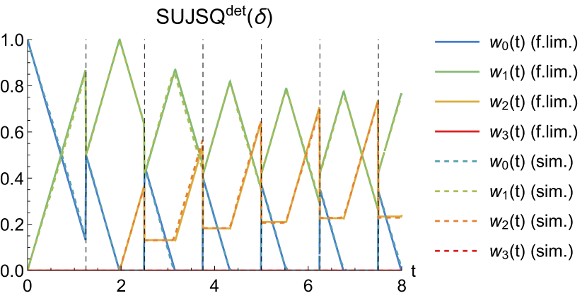
Figure 2. Numerical emulation of the fluid limit for SUJSQ${}^{\textup{det}}(0.85)$ and $\lambda=0.7$, accompanied by simulation results for $N=1000$, averaged over 10 runs.

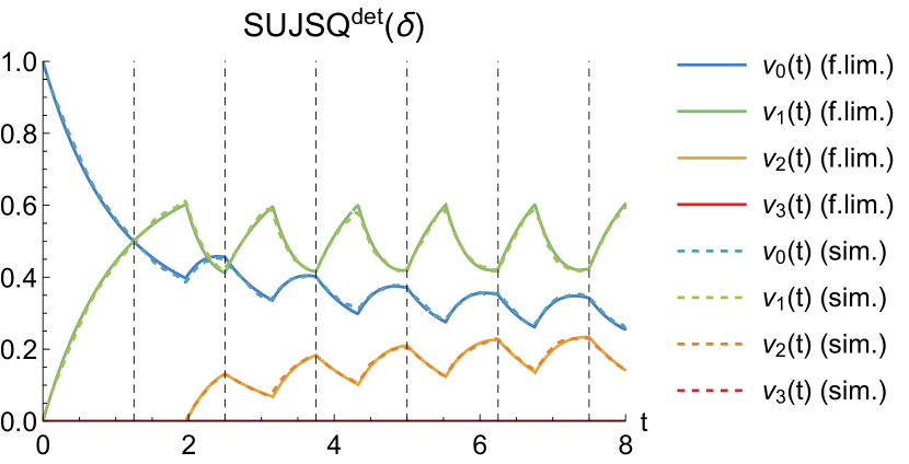
Figure 3. Numerical emulation of the fluid limit for SUJSQ${}^{\textup{det}}(0.85)$ and $\lambda=0.7$, accompanied by simulation results for $N=1000$, averaged over 10 runs.

4.1.2. Numerical illustration and comparison with simulation

Figures 3–5 show the fluid-limit trajectories $y(t)$ as governed by the differential equations in (1) for $\text{SUJSQ}^{\textup{det}}(\delta)$, along with (fluid-scaled) variables $y_{i,j}^{N}(t)$ obtained through stochastic simulation for a system with $N=1000$ servers and averaged over 10 runs. Observe that the simulation results are nearly indistinguishable from the fluid-limit trajectories, which is in line with broader findings concerning the accuracy of fluid and mean-field limits (Gast, 2017; Ying, 2016).

Update moments at times $1/\delta,2/\delta,\ldots$ are marked by vertical dotted lines. These time points can also be easily recognized by the jumps in the fraction of servers $w_{j}(t)$ that have queue estimate $j$. Moreover, the fraction of servers $v_{i}(t)$ with queue length $i$ is not differentiable in these points as well as other moments when the minimum queue estimate changes.

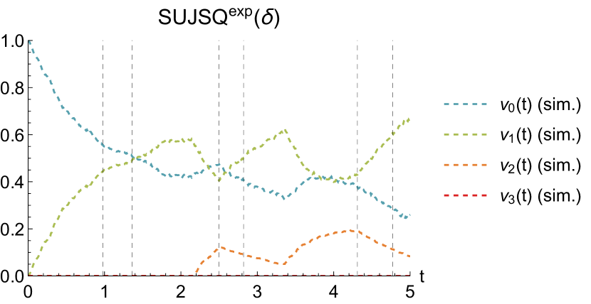
Figure 12. Simulation results for SUJSQ${}^{exp}(0.85)$.

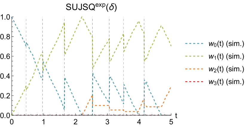
Figure 13. Simulation results for SUJSQ${}^{exp}(2.5)$.

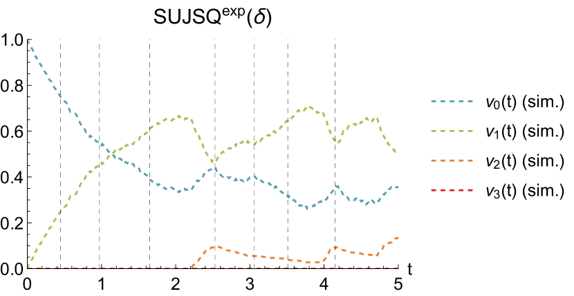
Figure 14. Simulation results for SUJSQ${}^{exp}(2.5)$.

Qualitatively similar results are observed for $\text{SUJSQ}^{\textup{exp}}(\delta)$, where the updates occur at irregular moments. The paths still follow similar saw-tooth patterns, and the dynamics between updates are identical, as reflected in the differential equations in (1). In particular, the fraction of servers with minimum queue estimate decreases linearly between updates, and the estimate drastically changes at update moments. The results are displayed in Figures 12–14, which are deferred to Appendix E because of space constraints.

In Figures 3 and 3, $\delta=0.85<\lambda/(1-\lambda)=7/3$, while $\delta=2.5>7/3$ in Figures 5 and 5. Since in the first scenario there are moments at which $w_{0}(t)$ is zero, some jobs are sent to servers with one job, so that servers sometimes have two jobs, which means that queueing does not vanish as $N\to\infty$. In contrast, in the second scenario, $w_{0}(t)$ is strictly positive at all times and no servers appear with two or more jobs, which implies that no queueing occurs at fluid level as $N\to\infty$. We will return to this dichotomy in Proposition 4.11.

4.2. Performance in the fluid limit

We will now use the fluid limit (1) to gain some insight in the performance of the $\text{SUJSQ}^{\textup{exp}}(\delta)$ scheme. (2) shows that no fixed point can exist as $w_{j}(t)$ has a non-zero constant derivative. We will establish however in Proposition 4.5 that for any positive update frequency the queue lengths on fluid scale are essentially bounded by a finite constant. Furthermore, in Proposition 4.11 we demonstrate that when the update frequency is above a specific threshold, queueing basically vanishes on fluid level in the long term.

Consider the average queue length on fluid scale, denoted and defined by

$$Q(t)=\sum_{i=0}^{\infty}iv_{i}(t)=\sum_{i=0}^{\infty}i\sum_{j=i}^{\infty}y_{i,j}(t).$$

Figure 4. Numerical emulation of the fluid limit for SUJSQ${}^{\textup{det}}(2.5)$ and $\lambda=0.7$, accompanied by simulation results for $N=1000$, averaged over 10 runs.

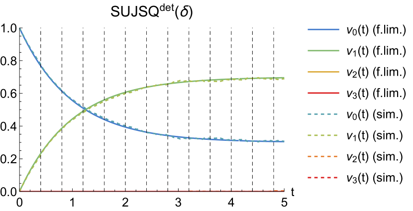
Figure 5. Numerical emulation of the fluid limit for SUJSQ${}^{\textup{det}}(2.5)$ and $\lambda=0.7$, accompanied by simulation results for $N=1000$, averaged over 10 runs.

Further define $z_{k}(t)=\sum_{i=k}^{\infty}v_{i}(t)$ as the fraction of servers with queue length $k$ or larger at time $t$ on fluid scale, and note that $Q(t)=\sum_{k=1}^{\infty}z_{k}(t)$. We will also refer to $Q(t)$ as the total queue ‘mass’ on fluid scale at time $t$, and introduce

$$\begin{split}Q^{\leq K}(t)&=\sum_{k=1}^{K}z_{k}(t)=\sum_{k=1}^{K}\sum_{i=k}^{\infty}v_{i}(t)\\ &=\sum_{i=1}^{K}\sum_{k=1}^{i}v_{i}(t)+\sum_{i=K+1}^{\infty}\sum_{k=1}^{K}v_{i}(t)\\ &=\sum_{i=1}^{K}iv_{i}(t)+\sum_{i=K+1}^{\infty}Kv_{i}(t)=\sum_{i=1}^{\infty}\min\{i,K\}v_{i}(t),\end{split}$$

and

$$\begin{split}Q^{>K}(t)&=Q(t)-Q^{\leq K}(t)=\sum_{k=K+1}^{\infty}z_{k}(t)=\sum_{k=K+1}^{\infty}\sum_{i=k}^{\infty}v_{i}(t)\\ &=\sum_{i=K+1}^{\infty}\sum_{k=K+1}^{i}v_{i}(t)=\sum_{i=K+1}^{\infty}(i-K)v_{i}(t)\end{split}$$

as the queue mass (weakly) below and (strictly) above level $K$, respectively.

The fluid-limit equation (1) yields the following expression for the derivative of $z_{k}(t)$ (in between updates),

$$\begin{split}\frac{dz_{k}(t)}{dt}=&\frac{d}{dt}\sum_{i=k}^{\infty}v_{i}(t)=\frac{d}{dt}\sum_{i=k}^{\infty}\sum_{j=i}^{\infty}y_{i,j}(t)=\sum_{i=k}^{\infty}\sum_{j=i}^{\infty}\frac{dy_{i,j}(t)}{dt}\\ =&\sum_{i=k}^{\infty}\sum_{j=i}^{\infty}\big{[}y_{i+1,j}(t)\mathds{1}\{i<j\}-y_{i,j}(t)\mathds{1}\{i>0\}\\ &+\lambda p_{i-1,j-1}(t)\mathds{1}\{i>0\}-\lambda p_{i,j}(t)\big{]}\\ =&\sum_{i=k}^{\infty}\big{[}v_{i+1}(t)-v_{i}(t)\mathds{1}\{i>0\}\\ &+\lambda\sum_{j=i}^{\infty}p_{i-1,j-1}(t)\mathds{1}\{i>0\}-\lambda\sum_{j=i}^{\infty}p_{i,j}(t)\big{]}\\ =&-v_{k}(t)\mathds{1}\{k>0\}+\lambda\sum_{j=k-1}^{\infty}p_{k-1,j}(t)\mathds{1}\{k>0\},\end{split}$$

and

(3) $$\begin{split}\frac{dQ^{>K}(t)}{dt}=&\frac{d}{dt}\sum_{k=K+1}^{\infty}z_{k}(t)=\sum_{k=K+1}^{\infty}\frac{dz_{k}(t)}{dt}\\ =&-\sum_{k=K+1}^{\infty}v_{k}(t)\mathds{1}\{k>0\}\\ &+\lambda\sum_{k=K+1}^{\infty}\sum_{j=k-1}^{\infty}p_{k-1,j}(t)\mathds{1}\{k>0\}\\ =&-z_{K+1}(t)+\lambda\sum_{k=K}^{\infty}\sum_{j=k}^{\infty}\frac{y_{k,j}(t)}{w_{j}(t)}\mathds{1}\{m(t)=j\}.\end{split}$$

This may be interpreted by noting that the queue mass above level $K$ increases due to arriving jobs being assigned to servers with queue length $K$ or larger and decreases due to jobs being completed by servers with queue length $K+1$ or larger. In particular, we find that

(4) $$\frac{dQ^{>K}(t)}{dt}=-z_{K+1}(t)$$

for all $K\geq m(t)+1$.

Taking $K=0$ and noting that $Q^{>0}(t)\equiv Q(t)$, we obtain

$$\frac{dQ(t)}{dt}=\lambda-z_{1}(t)=\lambda-[1-v_{0}(t)],$$

and thus

(5) $$Q(T)=Q(0)+\lambda T-\int_{0}^{T}[1-v_{0}(t)]dt.$$

This reflects that the average queue length on fluid scale at time $T$ is obtained by adding the number of arrivals $\lambda T$ during $[0,T]$ and subtracting the number of service completions, which corresponds to the cumulative fraction of busy servers $1-v_{0}(t)$.

The next lemma follows directly from (4), and shows that the queue mass above level $K$ decreases when the minimum queue estimate on fluid scale is strictly below $K$, so that there are no arrivals to servers with queue length $K$ or larger.

Lemma 4.1.

If $m(s)\leq K-1$ for all $s\in[0,t)$, then $Q^{>K}(t)\leq Q^{>K}(0)$.

We now proceed to derive a specific characterization of the decline in the queue mass above level $K$ when the minimum queue estimate on fluid scale is strictly below $K$.

For conciseness, denote

$$A(L,t)=\sum_{l=0}^{L}(L-l)\alpha_{l}(t)$$

and

$$B(L,t):=\sum_{l=0}^{L}l\alpha_{l}(t)+L\sum_{l=L+1}^{\infty}\alpha_{l}(t)$$

with $\alpha_{l}(t)=\frac{t^{l}}{l!}{\mathrm{e}}^{-t}$, and let $G$ be a Poisson random variable with parameter $t$. Note that $A(L,t)={\mathbb{E}}[\max\{L-G,0\}]$ and $B(L,t)={\mathbb{E}}[\min\{G,L\}]$ so that $A(L,t)+B(L,t)=L$, and in particular $B(L,t)\leq L$. Observe that $A(L,T)$ may be interpreted as the expected queue length after a time interval of length $T$ at a single server with initial queue length $L$, unit-exponential service times and no arrivals, while $B(L,T)$ may be interpreted as the expected number of service completions during that time period.

Lemma 4.2.

For any $K\geq 0$, $L\geq 1$, $t\geq 0$,

$$\begin{split}\int_{0}^{t}z_{K+1}(s)ds&\geq\left[Q^{\leq K+L}(0)-Q^{\leq K}(0)\right]\left[1-\frac{A(L,t)}{L}\right]\\ &=\frac{1}{L}\left[Q^{\leq K+L}(0)-Q^{\leq K}(0)\right]B(L,T).\end{split}$$

The proof of Lemma 4.2 involves a detailed analysis of $z_{K+1}(t)$. In the lemma special attention goes to the mass of jobs that are queued in positions $K+1$ up to $K+L$, represented by $Q^{\leq K+L}(0)-Q^{\leq K}(0)$. The decline in this mass is no less than the decline in a situation where the same total number of jobs reside with servers have either $0$ jobs or exactly $L$ jobs (so a fraction $[Q^{\leq K+L}(0)-Q^{\leq K}(0)]/L$ of the servers will have $L$ jobs). Finally, $A(L,t)$ represents the expected number of jobs that remain at time $t$ at each of the servers with $L$ jobs, while $B(L,t)$ represents the expected number of jobs that have been completed at time $t$ by each of these servers. These observations will be made rigorous in the proof in Appendix C.1.

The next lemma follows directly from (3) and (4) in conjunction with Lemma 4.2.

Lemma 4.3.

For any $K\geq 0$, $L\geq 1$, $t\geq 0$,

$$Q^{>K}(t)\leq\lambda t+Q^{>K+L}(0)+\frac{1}{L}\left[Q^{\leq K+L}(0)-Q^{\leq K}(0)\right]A(L,t),$$

or equivalently,

$$Q^{>K}(t)-Q^{>K}(0)\leq\lambda t-\frac{1}{L}\left[Q^{\leq K+L}(0)-Q^{\leq K}(0)\right]B(L,t).$$

If $m(y(s))\leq K-1$ for all $s\in[0,t)$, then for any $L\geq 1$

$$Q^{>K}(t)\leq Q^{>K+L}(0)+\frac{1}{L}\left[Q^{\leq K+L}(0)-Q^{\leq K}(0)\right]A(L,t),$$

or equivalently,

$$Q^{>K}(t)-Q^{>K}(0)\leq-\frac{1}{L}\left[Q^{\leq K+L}(0)-Q^{\leq K}(0)\right]B(L,t).$$

In particular, taking $L=1$,

$$\begin{split}Q^{>K}(t)&\leq Q^{>K+1}(0)+\left[Q^{\leq K+1}(0)-Q^{\leq K}(0)\right]{\mathrm{e}}^{-t}\\ &=Q^{>K+1}(0)+z_{K+1}(0){\mathrm{e}}^{-t},\end{split}$$

yielding

(6) $$Q^{>K}(t)\leq{\mathrm{e}}^{-t}Q^{>K}(0)+[1-{\mathrm{e}}^{-t}]Q^{>K+1}(0).$$

The next lemma provides a simple condition for the minimum queue estimate on fluid scale to remain strictly below $K$ throughout the interval $[0,t)$ in terms of $Q(0)$ and the proof is provided in Appendix C.2

Lemma 4.4.

If $Q(0)\leq K-\lambda t$, then $m(s)\leq K-1$ for all $s\in[0,t)$.

We will henceforth say that $L$ is large enough if

(7) $$\lambda T<\sigma(L;\lambda,T)=\left(1-\frac{\lambda T+1}{L}\right)B(L,T),$$

and define $s(\lambda,T)=\min\{L:\lambda T<\sigma(L;\lambda,T)\}$, which may be loosely thought of as the maximum queue length on fluid scale in the sense of the next proposition. Note that $\sigma(L;\lambda,T)\uparrow T$ as $L\to\infty$, ensuring that ${s}(\lambda,T)$ is finite for any $\lambda<1$.

Proposition 4.5 (Bounded queue length for $\text{SUJSQ}^{\textup{det}}(\delta)$).

For any initial state $y(0)$ with finite queue mass $Q(0)<\infty$, the fraction of servers on fluid scale with a queue length larger than $s(\lambda,T)$ vanishes over time. Additionally, if the initial queue mass $Q(0)$ is sufficiently small and the initial fraction of servers with a queue length larger than $s(\lambda,T)$ is zero, then that fraction will remain zero forever.

The proof of Proposition 4.5 leverages Lemma 4.2 and is organized as follows. For any initial state, we can show that either the mass in the tail, or the total mass is decreasing. Once one of the two is below a certain level, we show that the other decreases as well. We show this in two lemmas. From that point on, it is a back and forth between decreasing mass in the tail and decreasing total mass, which is described in the final lemma. The mass in the tail will decrease, such that the mass strictly above level $L^{*}=s(\lambda,T)$ will vanish.

Define

(8) $$\Delta=\left(1-\frac{\lambda T+1}{L^{*}}\right)B(L^{*},T)-\lambda T.$$

We now state two corollaries, which provide upper bounds for the total queue mass at time $T$. The proofs are based on Lemma 4.2 and provided in Appendices C.3 and C.4.

Corollary 4.6.

If $L$ is large enough and $Q(0)\geq L-1-\lambda T$, then

$$\begin{split}Q(T)&\leq Q(0)-\Delta+\frac{Q^{>L}(0)}{L}B(L,T)\\ &<Q(0)-\Delta+Q^{>L}(0).\end{split}$$

Corollary 4.7.

If $L$ is large enough and $Q(0)\leq L-1-\lambda T$, then

$$\begin{split}Q(T)&\leq L-1-\lambda T-\Delta+\frac{Q^{>L}(0)}{L}B(L,T)\\ &<L-1-\lambda T-\Delta+Q^{>L}(0).\end{split}$$

We now present Lemmas 4.8 and 4.9, which use Corollaries 4.6 and 4.7 and Lemmas 4.1, 4.3 and 4.4 to show that under certain conditions, the total queue mass as well as the mass above level $L$ strictly decrease.

Lemma 4.8.

If $L$ is large enough, $L-1-\lambda T\leq Q(0)\leq L-\lambda T$ and $Q^{>L}(0)<\Delta$, then

• $Q(T)<Q(0)-D$, where $D>0$, so $Q$ is strictly smaller at the next update,

• $Q^{>L}(T)\leq Q^{>L}(0)$, so $Q^{>L}$ remains strictly smaller than $\Delta$.

Proof.

The first statement follows from Corollary 4.6, with $D=\Delta/2-Q^{>L}(0)/2$. The second assertion follows from Lemmas 4.1 and 4.4. ∎

Lemma 4.9.

If $L$ is large enough, $Q(0)\leq L-1-\lambda T$ and $Q^{>L}(0)<\Delta$ then

• $Q(T)<L-1-\lambda T$, so $Q$ remains strictly smaller than $L-1-\lambda T$ at the next update,

• $Q^{>L}(T)\leq Q^{>L}(0)$, so $Q^{>L}$ remains strictly smaller than $\Delta$,

• $Q^{>L-1}(T)\leq cQ^{>L-1}(0)$ if $Q^{>L-1}(0)\geq\Delta$, where $c<1$, so $Q^{>L-1}$ is strictly decreasing by a constant factor over each update interval.

Proof.

The first statement follows from Corollary 4.7. The second assertion follows from Lemmas 4.1 and 4.4. The third statement holds for

$$c={\mathrm{e}}^{-T}+(1-{\mathrm{e}}^{-T})\frac{Q^{>L}(0)}{\Delta}<1$$

since the final portion of Lemma 4.3 in conjunction with Lemma 4.4 gives

$$\begin{split}\frac{Q^{>L-1}(T)}{Q^{>L-1}(0)}&\leq{\mathrm{e}}^{-T}+(1-{\mathrm{e}}^{-T})\frac{Q^{>L}(0)}{Q^{>L-1}(0)}\\ &\leq{\mathrm{e}}^{-T}+(1-{\mathrm{e}}^{-T})\frac{Q^{>L}(0)}{\Delta}.\end{split}$$

∎

Lemma 4.10.

If $L$ is large enough, $Q(0)\leq L-\lambda T$ and $Q^{>L}(0)<\Delta$, then there exists a finite time $\tau_{L}^{*}$ such that $Q(\tau_{L}^{*})\leq L-1-\lambda T$ and $Q^{>L-1}(\tau_{L}^{*})<\Delta$ (as defined in (8)).

Proof.

The proof is constructed by applying Lemmas 4.8 and 4.9 in succession. Since $Q(0)\leq L-\lambda T$ and $Q^{>L}(0)<\Delta$, Lemma 4.8 can be applied, so that $Q$ is strictly decreasing and eventually becomes smaller than $L-1-\lambda T$ while $Q^{>L}$ remains smaller than $\Delta$. Note that $D$ does not decrease after any iteration since $Q^{>L}(0)$ can only decrease. At that moment, Lemma 4.9 can be applied which shows that $Q^{>L-1}$ decreases by a constant factor over each update interval as long as $Q^{>L-1}$ is larger than $\Delta$. The constant factor $c$ does not increase after any iteration, and in fact only becomes smaller as $Q^{>L}(0)$ decreases. In other words, $Q^{>L-1}$ becomes smaller than $\Delta$ after finitely many updates, while $Q$ remains smaller than $L-1-\lambda T$ and $Q^{>L}$ smaller than $\Delta$. ∎

Proof of Proposition 4.5. Observe that the procedure in the proof of Lemma 4.10 can be performed as long as $L$ is large enough. The left-hand side of (7) is increasing in $L$ (as both factors are increasing in $L$), which shows that the condition (7) becomes tighter for smaller values of $L$. In fact, the mass above level $L^{*}$ will vanish, where $L^{*}$ is the lowest value of $L$ which is sufficiently large for (7) to hold, yielding the first statement of Proposition 4.5. The latter part follows directly from Lemma 4.8.

Finally, we stress that the lemma can also be applied when the maximum initial queue length is infinite, but the mass $Q(0)=\sum_{i=0}^{\infty}z_{i}(0)<\infty$ is finite. In that case, one can find a value for $\bar{L}$ such that $Q^{>\bar{L}}(0)=\sum_{i=\bar{L}}^{\infty}z_{i}(0)<\Delta$ (as the tail of a convergent series tends to zero) and $Q(0)\leq\bar{L}-\lambda T$. In that case, the lemma can be successively applied, starting from $\bar{L}$, which proves Proposition 4.5.

We now proceed to state the second main result in this section. Denote by $y^{*}$ the fluid state with $y_{0,0}^{*}=1-\lambda$, $y_{0,1}^{*}=0$, $y_{1,1}^{*}=\lambda$, and $y_{i,j}^{*}=0$ for all $j\geq i\geq 2$.

Proposition 4.11 (No-queueing threshold for $\delta$ in $\text{SUJSQ}^{\textup{det}}(\delta)$).

Suppose $\delta>\lambda/(1-\lambda)$, or equivalently, $T=1/\delta<(1-\lambda)/\lambda=1/\lambda-1$. Then $y^{*}$ is a fixed point of the fluid-limit process at update moments in the following sense:

1. If $y(0)=y^{*}$, then $y(kT)=y^{*}$ for all $k\geq 0$;

2. For any initial state $y(0)$ with $Q(0)<\infty$, $y(kT)\to y^{*}$ as $k\to\infty$.

Moreover, in case (a), $y_{0,0}(kT+t)=1-\lambda-\lambda t$, $y_{0,1}(kT+t)=\lambda t$, $y_{1,1}(kT+t)=\lambda$ for all $k\geq 0$, $t\in[0,T)$, and $y_{i,j}(t)=0$ for all $j\geq i\geq 2$, $t\geq 0$.
In case (b), $y_{0,0}(kT+t)\to 1-\lambda-\lambda t$, $y_{0,1}(kT+t)\to\lambda t$, $y_{1,1}(kT+t)\to\lambda$ for all $k\geq 0$, $t\in[0,T)$, and $y_{i,j}(t)\to 0$ for all $j\geq i\geq 2$, $t\geq 0$.

Loosely speaking, Proposition 4.11 implies that for $\delta\geq\lambda/(1-\lambda)$, in the long term the fraction of jobs that incur a non-zero waiting time vanishes. We note that in this regime, jobs are only sent to idle servers, which means that servers only need to send feedback whenever they are idle at an update moment. Since the fraction of idle servers in the fixed point is $1-\lambda$, a sparsified version of $\text{SUJSQ}^{\textup{det}}(\delta)$ will have a communication overhead of $\lambda$ per time unit or 1 message per job.

The next lemma, whose proof is presented in Appendix C.5, provides lower and upper bounds for the number of service completions on fluid level and the total queue mass, which play an instrumental role in the proof of Proposition 4.11. The bounds and proof arguments are similar in spirit to those of Lemma 4.2 with $K=0$, but involve crucial refinements by additionally accounting for service completions of arriving jobs.

Lemma 4.12.

If $v_{0}(0)\leq 1-\lambda$, then (i) $v_{0}(T)\leq 1-\lambda$.

If $v_{0}(0)\geq\lambda T$, then $\int_{0}^{T}[1-v_{0}(t)]dt$ is bounded from below by

$$\begin{split}&\lambda[T-1+{\mathrm{e}}^{-T}]+z_{1}(0)[1-{\mathrm{e}}^{-T}]+z_{2}(0)[1-{\mathrm{e}}^{-T}-T{\mathrm{e}}^{-T}]\\ =&\lambda T+[z_{1}(0)-\lambda][1-{\mathrm{e}}^{-T}]+z_{2}(0)[1-{\mathrm{e}}^{-T}-T{\mathrm{e}}^{-T}],\end{split}$$

so that in view of (5) (ii)

$$Q(T)\leq Q(0)-[z_{1}(0)-\lambda][1-{\mathrm{e}}^{-T}]-z_{2}(0)[1-{\mathrm{e}}^{-T}-T{\mathrm{e}}^{-T}],$$

and

$$Q(T)\geq Q(0)-[z_{1}(0)-\lambda][1-{\mathrm{e}}^{-T}]-z_{2}(0)T,$$

so that in view of (5) (iii),

$$\begin{split}\int_{0}^{T}[1-v_{0}(t)]dt&\leq\lambda[T-1+{\mathrm{e}}^{-T}]+z_{1}(0)[1-{\mathrm{e}}^{-T}]+z_{2}(0)T\\ &=\lambda T+[z_{1}(0)-\lambda][1-{\mathrm{e}}^{-T}]+z_{2}(0)T.\end{split}$$

If $v_{0}(0)<\lambda T$, then $\int_{0}^{T}[1-v_{0}(t)]dt$ is bounded from below by

$$\begin{split}&\lambda[T-1+{\mathrm{e}}^{-T}]+\hat{z}_{1}(0)[1-{\mathrm{e}}^{-T}]+\hat{z}_{2}(0)[1-{\mathrm{e}}^{-T}-T{\mathrm{e}}^{-T}]\\ =&\lambda T+[\hat{z}_{1}(0)-\lambda][1-{\mathrm{e}}^{-T}]+\hat{z}_{2}(0)[1-{\mathrm{e}}^{-T}-T{\mathrm{e}}^{-T}],\end{split}$$

so that in view of (5) (iv)

$$Q(T)\leq Q(0)-[\hat{z}_{1}(0)-\lambda][1-{\mathrm{e}}^{-T}]-\hat{z}_{2}(0)[1-{\mathrm{e}}^{-T}-T{\mathrm{e}}^{-T}],$$

with $\hat{z}_{i}(0)=\min\{z_{i}(0),1-\lambda T\}$, $i=1,2$.

We deduce that (v)

$$\begin{split}Q(T)\leq Q(0)&-\min\{1-v_{0}(0)-\lambda,1-\lambda T-\lambda\}[1-{\mathrm{e}}^{-T}]\\ &-\min\{z_{2}(0),1-\lambda T\}[1-{\mathrm{e}}^{-T}-T{\mathrm{e}}^{-T}],\end{split}$$

with $1-\lambda T-\lambda>0$.

Proof of Proposition 4.11.

We first consider case (a) with $y(0)=y^{*}$. The fluid-limit equations can then be explicitly solved to obtain $y_{0,0}(t)=1-\lambda-\lambda t$, $y_{0,1}(t)=\lambda t$, $y_{1,1}(t)=\lambda$, and $y_{i,j}(t)=0$ for all $j\geq i\geq 2$ for $t\in[0,T)$.

Since at an update moment $y_{0,0}(T)=y_{0,0}(T^{-})+y_{0,1}(T^{-})=1-\lambda$, $y_{1,1}(T)=y_{1,1}(T^{-})=\lambda$, and $y_{i,j}(t)=y_{i,j}(T^{-})=0$ for all $j\geq i\geq 2$, we obtain a strictly cyclic evolution pattern with $y(kT)=y^{*}$ for all $k\geq 0$, as well as $y_{0,0}(kT+t)=1-\lambda-\lambda t$, $y_{0,1}(kT+t)=\lambda t$, $y_{1,1}(kT+t)=\lambda$ for all $k\geq 0$ $t\in[0,T)$, and $y_{i,j}(t)=0$ for all $j\geq i\geq 2$, $t\geq 0$.

We now turn to case (b). First suppose that there exists a $k_{0}<\infty$ such that $v_{0}(k_{0}T)\leq 1-\lambda$. It then follows from statement (i) in Lemma 4.12 that $v_{0}(kT)\leq 1-\lambda$ for all $k\geq k_{0}$. Moreover, in view of statement (v) in Lemma 4.12 we have $Q((k+1)T)\leq Q(kT)-c\min\{\epsilon,\Delta\}-d\min\{z_{2}(kT),1-\lambda T\}$, with $c>0$ and $d>0$ when $v_{0}(kT)\leq 1-\lambda-\epsilon$ for any $\epsilon>0$. Thus, for any $\epsilon>0$ it can only occur finitely many times that $v_{0}(kT)\leq 1-\lambda-\epsilon$, and additionally for any $\delta>0$, it can only occur finitely many times that $z_{2}(kT)\geq\delta$, because otherwise $Q(kT)$ would eventually fall to zero, which would contradict $v_{0}(kT)\leq 1-\lambda$. Thus we conclude that $v_{0}(kT)\to 1-\lambda$ and $z_{2}(kT)\to 0$, which implies that $y(kT)\to y^{*}$ as $k\to\infty$ as stated.

Now suppose that there exists no $k_{0}<\infty$ such that $v_{0}(k_{0}T)\leq 1-\lambda$, i.e, $v_{0}(kT)>1-\lambda$ for all $k\geq 1$. Solving (1) then gives $\frac{d}{dt}w_{0}(t)=-\frac{d}{dt}w_{1}(t)=-\lambda$ and $m(t)=0$ for $t\in[kT,kT+v_{0}(kT)/\lambda]$, where $v_{0}(kT)/\lambda>T$. Lemma 4.3 with $K=1$, $L=1$ yields

$$Q^{>1}((k+1)T)\leq Q^{>1}(kT)-z_{2}(kT)[1-{\mathrm{e}}^{-T}].$$

Thus we must have $z_{2}(kT)\to 0$ as $k\to\infty$, because otherwise $Q^{>1}(kT)$ would eventually drop below zero, which would contradict the fact that it must always be positive. Hence, for any $\epsilon>0$, there exists $k_{\epsilon}$ such that $z_{2}(kT)\leq\epsilon(1-{\mathrm{e}}^{-T})/(2T)$ for all $k\geq k_{\epsilon}$,. Statement (iii) in Lemma 4.12 may then be invoked to obtain that for any $\epsilon>0$ and $k\geq k_{\epsilon}$ if $v_{0}(kT)\geq 1-\lambda+\epsilon\geq\lambda T$, then

$$Q((k+1)T)\geq Q(kT)+\frac{\epsilon}{2}\frac{1-{\mathrm{e}}^{-T}}{T}.$$

It follows that for any $\epsilon>0$, it can only occur finitely many times that $v_{0}(kT)\geq 1-\lambda+\epsilon$, as $Q(kT)$ is bounded since $Q^{>1}(kT)$ is decreasing (Lemma 4.1). Thus we conclude $v_{0}(kT)\to 1-\lambda$ and $z_{2}(kT)\to 0$ as $k\to\infty$, implying that $y(kT)\to y^{*}$ as $k\to\infty$ as stated.

∎

5. Asynchronous updates

In this section we turn to the fluid limit for asynchronous updates. As mentioned earlier, for non-exponential update intervals, the state variables $Y_{ij}$ would need to be augmented with continuous variables in order to obtain a Markovian state description. This would give rise to a measure-valued fluid-limit description, and involve heavy technical machinery, but provide little insight, and hence we will focus on the fluid limit for exponential update intervals. In Subsection 5.1 we provide a characterization of the fluid-limit trajectory, along with a heuristic explanation, numerical illustration and comparison with simulation. In Subsection 5.2 the fixed point of the fluid limit is determined (Proposition 5.1), which immediately shows that in stationarity queueing vanishes at fluid level for sufficiently high $\delta$ (Corollary 5.2) and also provides an upper bound for the queue length at fluid level for any given $\delta>0$ (Corollary 5.3).

5.1. Fluid-limit dynamics

In the case of synchronous updates, the minimum queue estimate $m(y^{N}(t))$ could never decrease between successive update moments. As a result, the amount of time $\int_{t_{0}}^{t}{\mathds{1}}{\{{\displaystyle m(Y^{N}(s))=j}\}}ds$ that the minimum queue length equals $j$ in between successive update moments converges to $\int_{t_{0}}^{t}\alpha_{j}(s)ds$, as $N\to\infty$, with $\alpha_{j}(t)={\mathds{1}}{\{{\displaystyle m(y(t))=j}\}}$ and can be directly expressed in terms of the minimum queue estimate on fluid scale.

In contrast, with asynchronous updates, the minimum queue estimate may drop at any time when an individual server with a queue length $i<m(y^{N}(t))$ sends an update at time $t$, and becomes the only server with a queue estimate below $m(y^{N}(t))$. Consequently, the amount of time $\int_{t_{0}}^{t}{\mathds{1}}{\{{\displaystyle m(Y^{N}(s))=j}\}}ds$ that the minimum queue length equals $j$ no longer tends to $\int_{t_{0}}^{t}\alpha_{j}(s)ds$ as $N\to\infty$, and may even have a positive derivative for $j<m(y(t))$, i.e., for queue values strictly smaller than the minimum queue estimate on fluid scale.

The fact that even in the limit the system may spend a non-negligible amount of time in states that are not directly visible on fluid scale severely complicates the characterization of the fluid limit. In order to handle this complication and describe the evolution of the fluid limit, it is convenient to define $u_{k}(t)=\delta\sum_{i=0}^{k-1}(k-i)v_{i}(t)$ as the fluid-scaled rate at which the dispatcher can assign jobs to servers with queue estimates below $k$ as a result of updates, with $v_{i}(t)=\sum_{l=i}^{\infty}y_{i,l}(t)$ representing the fraction of servers with queue length $i$ in fluid state $y$ at time $t$ as before.

We distinguish two cases, depending on whether $u_{m(t)}(t)$ $\leq\lambda$ or not, and additionally introduce $n(t)$, defined as $n(t)=m(t)$ in case $u_{m(t)}(t)\leq\lambda$, or $n(t)=\min\{n:u_{n}(t)>\lambda\}\leq m(t)-1$ otherwise. Then servers with a true queue length $i\leq n(t)-1$ will be assigned $n(t)-i$ jobs almost immediately after an update at time $t$, and then have both queue length and queue estimate $n(t)$. Incoming jobs will be assigned to servers with a queue estimate at most $n(t)-1$ at rate $u_{n(t)}(t)$ and to servers with queue estimate exactly equal to $n(t)$ at rate $\zeta(t)=\lambda-u_{n(t)}(t)$.

Then the fluid limit $y(t)$ satisfies the system of differential equations

(9) $$\begin{split}\frac{dy_{i,j}(t)}{dt}&=y_{i+1,j}(t)\mathds{1}\{i<j\}-y_{i,j}(t)\mathds{1}\{i>0\}\\ &+\zeta(t)q_{i-1,j-1}(t)\mathds{1}\{i>0\}-\zeta(t)q_{i,j}(t)\\ &+\delta\sum_{k=0}^{n(t)-1}v_{k}(t)\mathds{1}\{i=j=n(t)\}\\ &+\delta v_{i}(t)\mathds{1}\{i=j\geq n(t)\}-\delta y_{ij}(t),\end{split}$$

for all $i=0,1,\dots,j\geq n(t)$, where

$$q_{i,j}(t)=\frac{y_{i,j}(t)}{w_{j}(t)}\mathds{1}\{n(t)=j\}$$

denotes the fraction of jobs assigned to a server with queue length $i$ and queue estimate $j$ in fluid state $y$ among the ones that are assigned to a server with queue estimate at least $n(t)$, defined as function of the fluid state $y$ at time $t$ as above.

It can be checked that when $n(t)<m(t)$, the derivative of $\sum_{j=0}^{m(t)}w_{j}(t)$ is strictly positive, i.e., the fraction of servers with a queue estimate below $m(t)$ becomes positive, and the value of $m(t)$ instantly becomes equal to $n(t)$.

An informal outline of the derivation of the fluid limit as stated in (9) is provided in Appendix B.

5.1.1. Interpretation

The above system of differential equations may be intuitively interpreted as follows. The first two terms correspond to service completions at servers with $i+1$ and $i$ jobs, just like in (1). The third and fourth terms account for job assignments to servers with a queue estimate $m(t)$. The third term captures the resulting increase in the fraction of servers with queue estimate $m(t)+1$, while the fourth term captures the corresponding decrease in the fraction of servers with queue estimate $m(t)$.

The final three terms in (9) correspond to the updates from servers received at a rate $\delta$. The fifth term represents the increase in the fraction of servers with queue estimate $n(t)$ due to updates from servers with a queue length $k\leq n(t)-1$ which are almost immediately being assigned $n(t)-k$ jobs and then have both queue length $i=n(t)$ and queue estimate $j=n(t)$. The sixth term represents the increase in the fraction of servers with a queue estimate $j=n(t)$ or larger due to updates from servers with a queue length $i=j$. The final term represents the decrease in the number of servers with queue length $i$ and queue estimate $j$ due to updates.

Even though a non-zero fraction of the jobs are assigned to servers with a queue estimate below $n(t)$, these events are not directly visible at fluid level, and only implicitly enter the fluid limit through the thinned arrival rate $\zeta(t)$.

Summing the equations (9) over $i=0,1,\dots,j$ yields

$$\frac{dw_{j}(t)}{dt} =\zeta(t)[\mathds{1}\{n(t)=j-1\}-\mathds{1}\{n(t)=j\}]$$

$$+\delta[v_{j}(t)-w_{j}(t)]\mathds{1}\{j\geq n(t)\},$$

reflecting that servers with queue estimate $n(t)$ are assigned jobs, and thus flipped into servers with queue estimate $n(t)+1$, at rate $\zeta(t)$, and that servers with a queue estimate $j\geq n(t)$ are created at an effective rate $\delta[v_{j}(t)-w_{j}(t)]$ as a result of updates.

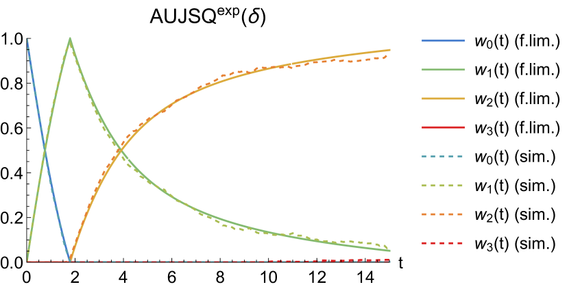
Figure 6. Numerical emulation of the fluid limit for AUJSQ${}^{\textup{exp}}(0.85)$ and $\lambda=0.7$, accompanied by simulation results with $N=1000$, averaged over 10 runs.

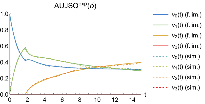
Figure 7. Numerical emulation of the fluid limit for AUJSQ${}^{\textup{exp}}(0.85)$ and $\lambda=0.7$, accompanied by simulation results with $N=1000$, averaged over 10 runs.

5.1.2. Numerical illustration and comparison with simulation

Figures 7-9 show the fluid-limit trajectories $y(t)$ as governed by the differential equations in (9) for $\text{AUJSQ}^{\textup{exp}}(\delta)$, through stochastic simulation for a system with $N=1000$ servers and averaged over 10 runs. Once again, the simulation results are nearly indistinguishable from the fluid-limit trajectories.

In contrast to the synchronous variants in Figures 3–5, the trajectories do not oscillate, but approach stable values, corresponding to the fixed point of the fluid-limit equations (9) which we will analytically determine in Proposition 5.1. In Figures 3 and 3 where $\delta=0.85$ is relatively low, we observe once again that $w_{2}(y(t))=w_{2}(t)$ and $v_{2}(y(t))=v_{2}(t)$ become strictly positive. In Figures 5 and 5 where $\delta=2.5$ is sufficiently large, all servers have either zero or one jobs in the limit, indicating that no queueing occurs.

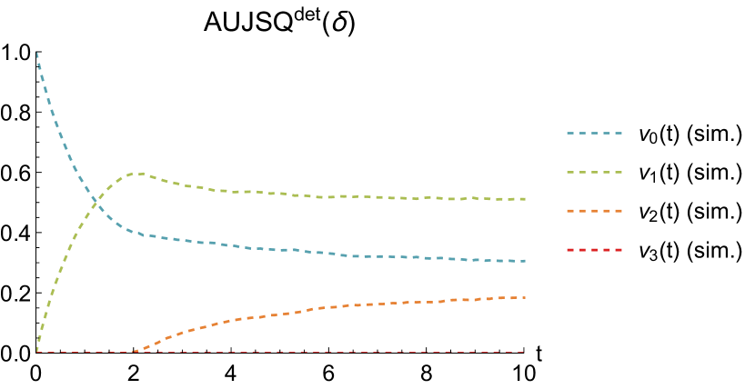
Figure 16. Simulation results for AUJSQ${}^{det}(0.85)$.

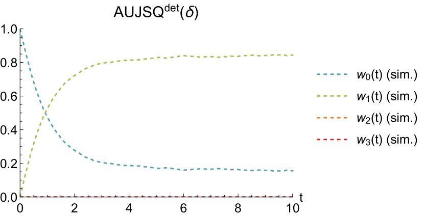
Figure 17. Simulation results for AUJSQ${}^{det}(2.5)$.

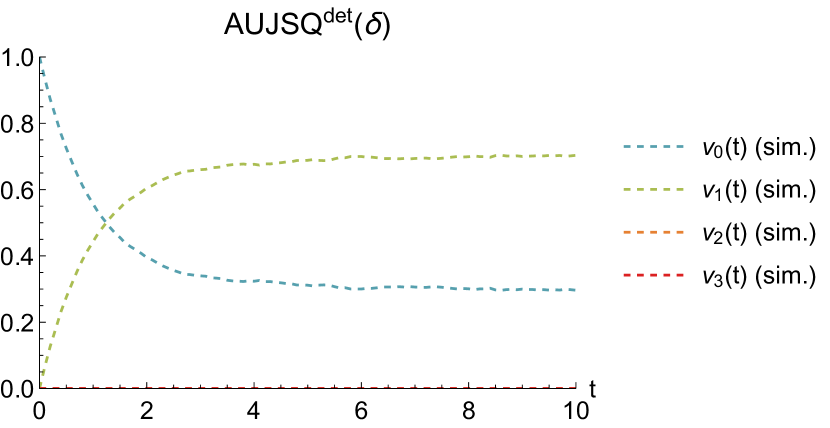
Figure 18. Simulation results for AUJSQ${}^{det}(2.5)$.

Qualitatively similar results are observed for $\text{AUJSQ}^{\textup{det}}(\delta)$, where the updates occur at strictly regular moments. The results are displayed in Figures 16–18, which are again relegated to Appendix F because of space limitations.

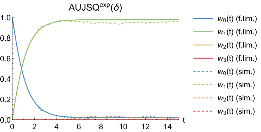
Figure 8. Numerical emulation of the fluid limit for AUJSQ${}^{\textup{exp}}(2.5)$ and $\lambda=0.7$, accompanied by simulation results with $N=1000$, averaged over 10 runs.

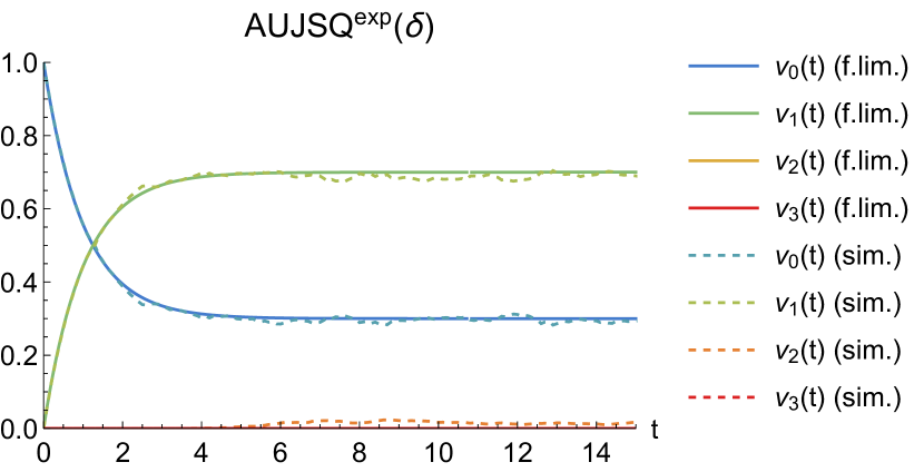
Figure 9. Numerical emulation of the fluid limit for AUJSQ${}^{\textup{exp}}(2.5)$ and $\lambda=0.7$, accompanied by simulation results with $N=1000$, averaged over 10 runs.

5.2. Fixed-point analysis

The next proposition identifies the fixed point of the fluid-limit equations (9) in terms of $m^{*}$, defined as

(10) $$\begin{split}m^{*}&=m(\lambda,\delta)=\min\left\{m:\lambda<1-\left(\frac{1}{1+\delta}\right)^{m+1}\right\}\\ &=\max\left\{m:\lambda\geq 1-\left(\frac{1}{1+\delta}\right)^{m}\right\}=\left\lfloor-\frac{\log(1-\lambda)}{\log(1+\delta)}\right\rfloor,\end{split}$$

which may be interpreted as the minimum queue estimate at fluid level in stationarity. For compactness, define $a=\frac{1}{1+\delta}$ and $b=\frac{1}{1+\delta+\nu}$.

Proposition 5.1 (Fixed point for $\text{AUJSQ}^{\textup{exp}}(\delta)$).

The fixed point of the fluid limit (9) is given by

$$y_{0,m^{*}}^{*} = \frac{ab^{m^{*}-1}\delta}{(1+\nu)(\delta+\nu)},$$

$$y_{i,m^{*}}^{*} = \frac{ab^{m^{*}-i}\delta}{1+\nu},\hskip 14.45377pti=1,\dots,m^{*},$$

$$y_{0,m^{*}+1}^{*} = a^{m^{*}+1}-\frac{a^{2}b^{m^{*}-1}\delta}{(1+\nu)(\delta+\nu)},$$

$$y_{1,m^{*}+1}^{*} = \delta\left(a^{m^{*}+1}-\frac{a^{2}b^{m^{*}-1}\delta}{(1+\nu)(\delta+\nu)}\right),$$

$$y_{i,m^{*}+1}^{*} = \delta\left(a^{m^{*}+2-i}-\frac{ab^{m^{*}+1-i}}{1+\nu}\right),\hskip 1.4457pti=2,\dots,m^{*}+1,$$

and $y_{i,j}^{*}=0$ when $j\neq m^{*},m^{*}+1$, where $\nu\geq 0$ is the unique solution of the equation $y_{0,m^{*}}+y_{0,m^{*}+1}=1-\lambda$, i.e.,

(11) $$h(\nu)=a^{m^{*}+1}+\frac{a^{2}b^{m^{*}-1}\delta^{2}}{(1+\nu)(\delta+\nu)}=1-\lambda.$$

In particular, if $\lambda=1-(1+\delta)^{-m^{*}}$, i.e.,

(12) $$m^{*}=-\frac{\log(1-\lambda)}{\log(1+\delta)},$$

then $\nu=0$, so

$$\begin{split}y_{0,m^{*}}^{*}&=\left(\frac{1}{1+\delta}\right)^{m^{*}}=1-\lambda,\\ y_{i,m^{*}}^{*}&=\delta\left(\frac{1}{1+\delta}\right)^{m^{*}+1-i}=\left(1-(1-\lambda)^{1/m^{*}}\right)(1-\lambda)^{\frac{m^{*}-i}{m^{*}}},\\ &\hskip 93.95122pti=1,\dots,m^{*},\end{split}$$

and $y_{i,m^{*}+1}^{*}=0$ for all $i=0,\dots,m^{*}+1$.

Note that $h(u)$ is strictly decreasing in $\nu$, with $\lim_{\nu\downarrow 0}h(\nu)=(\frac{1}{1+\delta})^{m^{*}}\leq 1-\lambda$, and $\lim_{\nu\to\infty}h(\nu)=(\frac{1}{1+\delta})^{m^{*}+1}<1-\lambda$, ensuring that $\nu\geq 0$ exists and is unique.

The result of Proposition 5.1 is obtained by setting the derivatives in (9) equal to zero, observing that $w_{j}(y^{*})=0$ for all $j\neq m^{*},m^{*}+1$, and then solving the resulting equations. The detailed proof arguments are presented in Appendix D.

Corollary 5.2 (No-queueing threshold for $\delta$ in $\text{AUJSQ}^{\textup{exp}}(\delta)$).

If the update frequency $\delta\geq\lambda/(1-\lambda)$, then $y_{i,j}^{*}=0$ for all $j\geq 2$, implying that queueing vanishes at fluid level in stationarity.

Corollary 5.2 immediately follows from (10) and Proposition 5.1, in which $m^{*}=0$ in case $\delta\geq\lambda/(1-\lambda)$ so that only $y^{*}_{0,0}$, $y^{*}_{0,1}$ and $y^{*}_{1,1}$ are strictly positive. In case of equality we have the scenario described in the last part of Proposition 5.1 where $y^{*}_{i,2}=0$ for all $i$. In case the many-server ($N\to\infty$) and stationary ($t\to\infty$) limits can be interchanged (a rigorous proof of that would involve establishing global asymptotic stability of the fluid limit, which is beyond the scope of the present paper), Corollary 5.2 implies that for $\delta\geq\lambda/(1-\lambda)$, the mean stationary waiting time under $\text{AUJSQ}^{\textup{exp}}(\delta)$ vanishes as $N\to\infty$.

Proposition 5.1 also yields an upper bound for the queue length at fluid level as stated in the next corollary.

Corollary 5.3 (Bounded queue length for $\text{AUJSQ}^{\textup{exp}}(\delta)$).

The queue length at fluid level in stationarity has bounded support on $\{0,\dots,$ $m(\lambda,\delta)+1\}$ for any $\lambda<1$ and $\delta>0$.

First of all, note that in order for queueing to vanish, it is required that $m(\lambda,\delta)=0$ or $m(\lambda,\delta)=1$ and $\nu=0$, i.e., $\delta\geq\lambda/(1-\lambda)$, which coincides with the threshold for $\delta$ in $\text{SUJSQ}^{\textup{det}}(\delta)$ as identified in Proposition 4.11. Also, the upper bound $m(\lambda,\delta)+1$ tends to infinity as $\delta$ approaches zero, reflecting that for any fixed arrival rate $\lambda$, even arbitrarily low, the maximum queue length grows without bound as the update frequency vanishes.

At the same time, for any positive $\delta>0$, $m(\lambda,\delta)$ is finite for any fixed $\lambda<1$, and only grows as $\log(1/(1-\lambda))$ as $\lambda\uparrow 1$ rather than $1/(1-\lambda)$ as in the absence of any queue feedback. Thus, even an arbitrarily low update frequency ensures that the queue length has bounded support and behaves far more benignly in a high-load regime at fluid level. This powerful property resembles an observation in work of Tsitsiklis & Xu (Tsitsiklis and Xu, 2012, 2013) in the context of a dynamic scheduling problem where even a minuscule degree of resource pooling yields a fundamentally different behavior on fluid scale.

5.2.1. Number of jobs in the system

The average queue length in the fixed point $\tilde{q}$ is

(13) $$\begin{split}&\tilde{q}=\sum_{i=1}^{m^{*}}iy_{i,m^{*}}^{*}+\sum_{i=1}^{m^{*}+1}iy_{i,m^{*}+1}^{*}\\ &=\frac{\delta+a^{m^{*}+1}+\delta m^{*}-1}{\delta}+\frac{a^{2}\delta\left(-\delta+b^{m^{*}}-1\right)}{b(1+\nu)(\delta+v)}\\ &\overset{\eqref{eq:h}}{=}m^{*}+1+\frac{a^{m^{*}+1}-1}{\delta}+\frac{1-\lambda-a^{m^{*}+1}}{\delta}-\frac{a(1+\delta+\nu)\delta}{(1+\nu)(\delta+\nu)}\\ &=m^{*}+1-\lambda/\delta-\frac{(1+\delta+\nu)\delta}{(1+\delta)(1+\nu)(\delta+\nu)}\geq m^{*}-\lambda/\delta.\end{split}$$

In case of (12), the average queue length is simply $\tilde{q}=m^{*}+1-\lambda/\delta-1$ $=m(\lambda,\delta)-\lambda/\delta$, reflecting that the average number of job arrivals equals the average number of job completions over the course of an update interval, starting with $m^{*}=m(\lambda,\delta)$ jobs.

Figure 10 plots the average queue length in the fixed point given by (13) as function of the update frequency $\delta$ for $\lambda=0.8$. We observe that the average queue length monotonically decreases with the update frequency, as expected, and is indeed contained between $m^{*}-\lambda/\delta$ and $m^{*}+1-\lambda/\delta$.

It then follows from the definition of $m^{*}=m(\lambda,\delta)$ that $\tilde{q}\to\infty$ as $\delta\downarrow 0$ for any $\lambda<1$, which indicates that $\text{AUJSQ}^{\textup{det}}(\delta)$ may perform arbitrarily badly in the ultra-low feedback regime, confirming the observations in Subsection 1.

5.2.2. Bound on the queue length for $\text{AUJSQ}^{\textup{det}}(\delta)$

As noted earlier, the fluid-limit trajectory for $\text{AUJSQ}^{\textup{det}}(\delta)$ involves a measure-valued process and is difficult to describe. However, in a similar spirit as for $\text{AUJSQ}^{\textup{exp}}(\delta)$, the value of $m^{*}$ can be characterized as the largest integer for which

$$\left(\sum_{i=1}^{m}i\frac{(1/\delta)^{i}}{i!}\text{e}^{-1/\delta}+m\sum_{i=m+1}^{\infty}\frac{(1/\delta)^{i}}{i!}\text{e}^{-1/\delta}\right)\leq\lambda/\delta,$$

expressing that the average number of job arrivals should be larger than or equal to the average number of job completions over the course of an update interval, starting with $m^{*}$ jobs. While the above equation cannot easily be solved in closed form, it is not difficult to show that the inequality is weaker than (10), i.e., the value of $m^{*}$ is lower than for $\text{AUJSQ}^{\textup{exp}}(\delta)$, confirming the superiority of $\text{AUJSQ}^{\textup{det}}(\delta)$ observed in the simulation results in Subsection 1. It is further worth observing the strong similarity of the above inequality with Proposition 4.5 governing the queue length upper bound for $\text{SUJSQ}^{\textup{det}}(\delta)$.

Figure 10. Values of $\tilde{q}$ for $\lambda=0.7$ and different values of $\delta$.

6. Conclusions

We have introduced and analyzed a novel class of hyper-scalable load balancing algorithms that only involve minimal communication overhead and yet deliver excellent performance. In the proposed schemes, the various servers provide occasional queue status notifications so as to guide the dispatcher in directing incoming jobs to relatively short queues.

We have demonstrated that the schemes markedly outperform JSQ($d$) policies with a comparable overhead, and can drive the waiting time to zero in the many-server limit with just one message per job. The proposed schemes show their core strength and outperform sparsified JIQ versions in the sparse feedback regime with less than one message per job, which is particularly pertinent from a scalability viewpoint.

In order to further explore the performance in the many-server limit, we investigated fluid limits for synchronous as well as asynchronous exponential update intervals. We used the fluid limits to obtain upper bounds for the stationary queue length as function of the load and update frequency. We also revealed a striking dichotomy in the ultra-low feedback regime where the mean waiting time tends to a constant in the synchronous case, but grows without bound in the asynchronous case. Extensive simulation experiments are conducted to support the analytical results, and indicate that the fluid-limit asymptotics are remarkable accurate.

In the present paper we have adopted common Markovian assumptions, and in future work we aim to extend the results to non-exponential and possibly heavy-tailed distributions. We also intend to pursue schemes that may dynamically suppress updates or selectively refrain from updates at pre-scheduled epochs to convey implicit information, and reduce the communication overhead yet further.

Appendix A Derivation sketch of fluid limit (1) for synchronous updates.

We now provide an informal outline of the derivation of the fluid limit for synchronous updates as stated in (1). Let $A_{i,j}(t)$ and $S_{i,j}(t)$ denote unit-rate Poisson processes, $j\geq i\geq 0$, all independent.

The system dynamics (in between successive update moments) may then be represented as (see for instance (Pang et al., 2007))

$$\begin{split}Y_{i,j}^{N}(t)=&~{}Y_{i,j}^{N}(t_{0})+S_{i+1,j}\left(\int_{t_{0}}^{t}Y_{i+1,j}^{N}(s)ds\right){\mathds{1}}{\left\{{\displaystyle i<j}\right\}}\\ &-S_{i,j}\left(\int_{t_{0}}^{t}Y_{i,j}^{N}(s)ds\right){\mathds{1}}{\left\{{\displaystyle i>0}\right\}}\\ &+A_{i-1,j-1}\left(\lambda N\int_{t_{0}}^{t}p_{i-1,j-1}(Y^{N}(s))ds\right){\mathds{1}}{\left\{{\displaystyle i>0}\right\}}\\ &-A_{i,j}\left(\lambda N\int_{t_{0}}^{t}p_{i,j}(Y^{N}(s))ds\right),\end{split}$$

with $p_{i,j}(Y)=\frac{Y_{i,j}}{\sum_{k=0}^{j}Y_{k,j}}{\mathds{1}}{\left\{{\displaystyle j=m(Y)}\right\}}$.

Dividing by $N$ and rewriting in terms of the fluid-scaled variables $y_{i,j}^{N}(t)=\frac{1}{N}Y_{i,j}^{N}(t)$, we obtain

(14) $$\begin{split}y_{i,j}^{N}(t)=&~{}y_{i,j}^{N}(t_{0})\\ &+\frac{1}{N}S_{i+1,j}\left(N\int_{t_{0}}^{t}y_{i+1,j}^{N}(s)ds\right){\mathds{1}}{\left\{{\displaystyle i<j}\right\}}\\ &-\frac{1}{N}S_{i,j}\left(N\int_{t_{0}}^{t}y_{i,j}^{N}(s)ds\right){\mathds{1}}{\left\{{\displaystyle i>0}\right\}}\\ &+\frac{1}{N}A_{i-1,j-1}\left(\lambda N\int_{t_{0}}^{t}p_{i-1,j-1}(Y^{N}(s))ds\right){\mathds{1}}{\left\{{\displaystyle i>0}\right\}}\\ &-\frac{1}{N}A_{i,j}\left(\lambda N\int_{t_{0}}^{t}p_{i,j}(Y^{N}(s))ds\right).\end{split}$$

Now introduce

$$\tilde{S}_{k,l}(u):=S_{k,l}(u)-u,~{}~{}~{}\tilde{A}_{k,l}(u):=A_{k,l}(u)-u,$$

and observe that $\tilde{S}_{k,l}(\cdot)$ and $\tilde{A}_{k,l}(\cdot)$ are martingales. By standard arguments it can be shown that both $\frac{1}{N}\tilde{S}_{k,l}(N\int_{t_{0}}^{t}y_{k,l}^{N}(s)ds)$ and $\frac{1}{N}\tilde{A}_{k,l}(\lambda N\int_{t_{0}}^{t}p_{k,l}(Y^{N}(s))ds)$ converge to zero as $N\to\infty$.

Exploiting the fact that the minimum queue estimate $m(Y^{N}(t))$ cannot decrease in between successive update moments, it can also be established that

$$\int_{t_{0}}^{t}p_{k,l}(Y^{N}(s))ds\to\int_{0}^{t}p_{k,l}(s)ds,$$

as $N\to\infty$, with $p_{k,l}(y)=\frac{y_{k,l}}{w_{l}(y)}{\mathds{1}}{\left\{{\displaystyle m(y)=l}\right\}}$ as defined earlier.

Taking the limit for $N\to\infty$ in (14), we conclude that any (weak) limit $\{y_{i,j}(t)\}_{t\geq 0}$ of the sequence $\left(\{y_{i,j}^{N}(t)\}_{t\geq 0}\right)_{N\geq 1}$ in between successive update moments must satisfy

$$\begin{split}y_{i,j}(t)=&~{}y_{i,j}(t_{0})+\int_{t_{0}}^{t}y_{i+1,j}(s)ds{\mathds{1}}{\left\{{\displaystyle i<j}\right\}}-\int_{t_{0}}^{t}y_{i,j}(s)ds{\mathds{1}}{\left\{{\displaystyle i>0}\right\}}\\ &+\lambda\int_{t_{0}}^{t}p_{i-1,j-1}(y(s))ds{\mathds{1}}{\left\{{\displaystyle i>0}\right\}}-\lambda\int_{t_{0}}^{t}p_{i,j}(y(s))ds,\end{split}$$

with $y_{i,j}(0)=y_{i,j}^{\infty}$.

Rewriting the latter integral equation in differential form yields (1).

Appendix B Derivation sketch of fluid limit (1) for asynchronous updates.

We now provide an informal outline of the derivation of the fluid limit as stated in (9). Let $A_{i,j}(t)$, $B_{i,j}(t)$ and $S_{i,j}(t)$ denote unit-rate Poisson processes, $j\geq i\geq 0$, all independent. The system dynamics may then be represented as (Pang et al., 2007)

$$\begin{split}Y_{i,j}^{N}(t)=&~{}Y_{i,j}^{N}(0)+S_{i+1,j}\left(\int_{0}^{t}Y_{i+1,j}^{N}(s)ds\right){\mathds{1}}{\left\{{\displaystyle i<j}\right\}}\\ &-S_{i,j}\left(\int_{0}^{t}Y_{i,j}^{N}(s)ds\right){\mathds{1}}{\left\{{\displaystyle i>0}\right\}}\\ &+A_{i-1,j-1}\left(\lambda N\int_{0}^{t}p_{i-1,j-1}(Y^{N}(s))ds\right){\mathds{1}}{\left\{{\displaystyle i>0}\right\}}\\ &-A_{i,j}\left(\lambda N\int_{0}^{t}p_{i,j}(Y^{N}(s))ds\right)\\ &+\sum_{k=j}^{\infty}B_{i,k}\left(\delta\int_{0}^{t}Y_{i,k}^{N}(s)ds\right){\mathds{1}}{\left\{{\displaystyle i=j}\right\}}\\ &-B_{i,j}\left(\delta\int_{0}^{t}Y_{i,j}^{N}(s)ds\right),\end{split}$$

with $p_{i,j}(Y)$ as before. Dividing by $N$ and rewriting in terms of the fluid-scaled variables $y_{i,j}^{N}(t)=\frac{1}{N}Y_{i,j}^{N}(t)$, we obtain

(15) $$\begin{split}y_{i,j}^{N}(t)&=~{}y_{i,j}^{N}(0)+\frac{1}{N}S_{i+1,j}\left(N\int_{0}^{t}y_{i+1,j}^{N}(s)ds\right){\mathds{1}}{\left\{{\displaystyle i<j}\right\}}\\ &-\frac{1}{N}S_{i,j}\left(N\int_{0}^{t}y_{i,j}^{N}(s)ds\right){\mathds{1}}{\left\{{\displaystyle i>0}\right\}}\\ &+\frac{1}{N}A_{i-1,j-1}\left(\lambda N\int_{0}^{t}p_{i-1,j-1}^{N}(Y^{N}(s))\right){\mathds{1}}{\left\{{\displaystyle i>0}\right\}}\\ &-\frac{1}{N}A_{i,j}\left(\lambda N\int_{0}^{t}p_{i,j}^{N}(Y^{N}(s))ds\right)\\ &+\frac{1}{N}\sum_{k=j}^{\infty}B_{i,k}\left(\delta N\int_{0}^{t}y_{i,k}^{N}(s)ds\right){\mathds{1}}{\left\{{\displaystyle i=j}\right\}}\\ &-\frac{1}{N}B_{i,j}\left(\delta N\int_{0}^{t}y_{i,j}^{N}(s)ds\right).\end{split}$$

Now introduce

$$\tilde{S}_{k,l}(u):=S_{k,l}(u)-u,~{}~{}\tilde{A}_{k,l}(u):=A_{k,l}(u)-u,~{}~{}\tilde{B}_{k,l}(u):=B_{k,l}(u)-u,$$

and observe that $\tilde{S}_{k,l}(\cdot)$, $\tilde{A}_{k,l}(\cdot)$ and $\tilde{B}_{k,l}(\cdot)$ are martingales. By standard arguments it can be shown that

$$\begin{split}&\frac{1}{N}\tilde{S}_{k,l}\left(N\int_{0}^{t}y_{k,l}^{N}(s)ds\right),\\ &\frac{1}{N}\tilde{A}_{k,l}\left(\lambda N\int_{0}^{t}p_{k,l}(Y^{N}(s))ds\right),\\ &\frac{1}{N}\tilde{B}_{k,l}\left(\delta N\int_{0}^{t}y_{k,l}^{N}(s)ds\right)\end{split}$$

each converge to zero as $N\to\infty$.

Adopting time-scale separation arguments as developed by Hunt & Kurtz (Hunt and Kurtz, 1994), it can be established that

$$\lambda\int_{0}^{t}p_{i,j}(Y^{N}(s))ds\to\int_{0}^{t}\alpha_{i,j}(s)ds$$

as $N\to\infty$, where the coefficients $\alpha_{i,j}(\cdot)$ satisfy

$$\alpha_{i,j}(t)=\left\{\begin{array}[]{ll}0&i<j<n(t),\\ \lambda\pi_{j}(t)&i=j<n(t),\\ \lambda\frac{y_{i,j}(t)}{w_{j}(y(t))}\pi_{n(t)}(t)&i\leq j=n(t),\\ 0&i\leq j>n(t).\end{array}\right.$$

The coefficients $\pi_{j}(t)$ may be interpreted as the fraction of time that the pre-limit minimum queue estimate equals $j\leq n(t)$ when the minimum queue estimate at fluid level is $n(t)$, and satisfy the relationship

$$\lambda\pi_{j}(t)=\lambda\pi_{j-1}(t)+\delta v_{j}(y(t))$$

for all $j=1,\dots,n(t)-1$, along with the normalization condition $\sum_{j=0}^{n(t)}\pi_{j}(t)=1$.

Thus, we obtain

$$\lambda\pi_{j}(t)=\delta\sum_{k=0}^{j}v_{k}(y(t)),$$

for all $j=0,\dots,n(t)-1$, and

$$\begin{split}\lambda\pi_{n(t)}(t)&=\lambda(1-\sum_{j=0}^{n(t)-1}\pi_{j}(t))=\lambda-\delta\sum_{j=0}^{n(t)-1}\sum_{k=0}^{j}v_{k}(y(t))\\ &=\lambda-\delta\sum_{i=0}^{n(t)-1}(n(t)-i)v_{i}(y(t))=\zeta(y(t)).\end{split}$$

We deduce that

$$\alpha_{i,j}(t)={\mathds{1}}{\left\{{\displaystyle i=j}\right\}}\delta\sum_{k=0}^{j}v_{k}(y(t)){\mathds{1}}{\left\{{\displaystyle j<n(t)}\right\}}+q_{i,j}(y(t)\zeta(y(t)),$$

with $q_{i,j}(y)=\frac{y{i,j}}{w_{j}(y)}{\mathds{1}}{\left\{{\displaystyle n(y)=j}\right\}}$ as before, yielding

$$\begin{split}&\int_{0}^{t}\alpha_{i-1,j-1}(s)ds-\int_{0}^{t}\alpha_{i,j}(s)ds\\ =&\int_{0}^{t}q_{i-1,j-1}(y(s))\zeta(y(s))ds-\int_{0}^{t}q_{i,j}(y(s))\zeta(y(s))ds\\ &+{\mathds{1}}{\left\{{\displaystyle i=j}\right\}}\delta\sum_{k=0}^{j-1}v_{k}(y(s)){\mathds{1}}{\left\{{\displaystyle j=n(s)}\right\}}ds\\ &-{\mathds{1}}{\left\{{\displaystyle i=j}\right\}}\delta\int_{0}^{t}v_{j}(y(s)){\mathds{1}}{\left\{{\displaystyle j<n(s)}\right\}}ds.\end{split}$$

Thus we obtain

(16) $$\begin{split}&\lambda\int_{0}^{t}p_{i-1,j-1}(Y^{N}(s))ds{\mathds{1}}{\left\{{\displaystyle i>0}\right\}}-\lambda\int_{0}^{t}p_{i,j}(Y^{N}(s))ds\to\\ &~{}~{}\int_{0}^{t}q_{i-1,j-1}(y(s))\zeta(y(s))ds{\mathds{1}}{\left\{{\displaystyle i>0}\right\}}-\int_{0}^{t}q_{i,j}(y(s))\zeta(y(s))ds\\ &~{}~{}+{\mathds{1}}{\left\{{\displaystyle i=j}\right\}}\delta\sum_{k=0}^{j-1}v_{k}(y(s)){\mathds{1}}{\left\{{\displaystyle j=n(y(s))}\right\}}ds\\ &~{}~{}-{\mathds{1}}{\left\{{\displaystyle i=j}\right\}}\delta\int_{0}^{t}v_{j}(y(s)){\mathds{1}}{\left\{{\displaystyle j<n(y(s))}\right\}}ds,\end{split}$$

as $N\to\infty$, with $\zeta(y)=\lambda-\delta\sum_{l=0}^{n(y)}(n(y)-l)v_{l}(y)$ and $q_{i,j}(y)=\frac{y_{i,j}}{w_{j}(y)}{\mathds{1}}{\left\{{\displaystyle n(y)=j}\right\}}$ as defined earlier.

Taking the limit for $N\to\infty$ in (15), and noting that

$$\begin{split}&{\mathds{1}}{\left\{{\displaystyle i=j}\right\}}\delta\int_{0}^{t}v_{i}(y(s))ds-{\mathds{1}}{\left\{{\displaystyle i=j}\right\}}\delta\int_{0}^{t}v_{j}(y(s)){\mathds{1}}{\left\{{\displaystyle j<n(y(s))}\right\}}ds\\ &=\delta\int_{0}^{t}v_{i}(y(s)){\mathds{1}}{\left\{{\displaystyle i=j\geq n(y(s))}\right\}},\end{split}$$

we conclude that any (weak) limit $\{y_{i,j}(t)\}_{t\geq 0}$ of the sequence $(\{y_{i,j}^{N}(t)\}_{t\geq 0})_{N\geq 1}$ must satisfy

$$\begin{split}&y_{i,j}(t)=y_{i,j}(0)+\int_{0}^{t}y_{i+1,j}(s)ds{\mathds{1}}{\left\{{\displaystyle i<j}\right\}}-\int_{0}^{t}y_{i,j}(s)ds{\mathds{1}}{\left\{{\displaystyle i>0}\right\}}\\ &~{}+\lambda\int_{0}^{t}q_{i-1,j-1}(y(s))\zeta_{j-1}(y(s))ds{\mathds{1}}{\left\{{\displaystyle i>0}\right\}}\\ &~{}-\lambda\int_{0}^{t}q_{i,j}(y(s))\zeta_{j}(y(s))ds+\delta\sum_{k=0}^{i-1}\int_{0}^{t}v_{k}(y(s)){\mathds{1}}{\left\{{\displaystyle i=j=n(y)}\right\}}ds\\ &~{}+\delta\int_{0}^{t}v_{i}(y(s)){\mathds{1}}{\left\{{\displaystyle i=j\geq n(y(s))}\right\}}-\delta\int_{0}^{t}y_{i,j}(s)ds,\end{split}$$

with $y_{i,j}(0)=y_{i,j}^{\infty}$. Rewriting the latter integral equation in differential form yields (9).

Appendix C Proofs of Section 4.2

C.1. Proof of Lemma 4.2

Let $\tilde{y}_{i,j}(t)$, $i=0,1,\dots,j$, $j\geq 0$, be the solution to the fluid-limit equation (1) with $\lambda=0$, i.e.,

$$\frac{\tilde{y}_{i,j}(t)}{dt}=\tilde{y}_{i+1,j}(t)\mathds{1}\{i<j\}-\tilde{y}_{i,j}(t)\mathds{1}\{i>0\},$$

with initial conditions $\tilde{y}_{i,i}(0)=v_{i}(0)$ and $\tilde{y}_{i,j}(0)=0$ for all $j\geq i+1$, $i\geq 0$. The solution $\tilde{y}_{i,j}(t)$ may be interpreted as the fluid limit in the absence of any arrivals, and it is easily verified that

$$\tilde{y}_{i,j}(t)=v_{j}(0)\frac{t^{j-i}}{(j-i)!}{\mathrm{e}}^{-t},$$

for all $i=1,2,\dots,j$, and

$$\tilde{y}_{0,j}(t)=v_{j}(0)\sum_{k=j}^{\infty}\frac{t^{k}}{k!}{\mathrm{e}}^{-t},$$

$j\geq 0$. Further introduce $\tilde{v}_{i}(t)=\sum_{j=i}^{\infty}\tilde{y}_{i,j}(t)$, $\tilde{z}_{k}(t)=\sum_{i=k}^{\infty}\tilde{v}_{i}(t)$, $\tilde{Q}^{>K}(t)=\sum_{k=K+1}^{\infty}\tilde{z}_{k}(t)$, and note from (3) that

(17) $$\frac{d\tilde{Q}^{>K}(t)}{dt}=-\tilde{z}_{K+1}(t).$$

We will first establish that $\tilde{z}_{k}(t)\leq z_{k}(t)$ for all $k\geq 0$, $t\in[0,T)$, reflecting that the fraction of servers with queue length $k$ or larger on fluid scale is no less than what it would be in the absence of any arrivals. Suppose that were not the case, and let $t_{0}\in[0,T)$ be the first time when that inequality is about to be violated for some $k_{0}>0$. Then we must have $z_{k_{0}}(t_{0})=\tilde{z}_{k_{0}}(t_{0})$, implying $v_{k_{0}}(t_{0})=z_{k_{0}}(t_{0})-z_{k_{0}+1}(t_{0})\leq\tilde{z}_{k_{0}}(t_{0})-\tilde{z}_{k_{0}+1}(t_{0})=\tilde{v}_{k_{0}}(t_{0})$, since $\tilde{z}_{k_{0}+1}(t_{0})\leq z_{k_{0}+1}(t_{0})$. Now observe that

$$\frac{dz_{k_{0}}(t)}{dt}\mid_{t=t_{0}}=-v_{k_{0}}(t_{0})+\lambda\sum_{j=k_{0}-1}^{\infty}p_{k_{0}-1,j}(t_{0})\geq-v_{k_{0}}(t_{0}),$$

while

$$\frac{d\tilde{z}_{k_{0}}(t)}{dt}\mid_{t=t_{0}}=-\tilde{v}_{k_{0}}(t_{0})\leq-v_{k_{0}}(t_{0})\leq\frac{dz_{k_{0}}(t)}{dt}.$$

Hence $z_{k_{0}}(t)$ cannot fall below $\tilde{z}_{k_{0}}(t)$ at (just after) $t_{0}$, contradicting the initial supposition in which $t_{0}$ would be the first time that the inequality is about to be violated.

Invoking (17), we obtain

$$\begin{split}\int_{s=0}^{t}z_{K+1}(s)ds&\geq\int_{s=0}^{t}\tilde{z}_{K+1}(s)ds=Q^{>K}(0)-\tilde{Q}^{>K}(t)\\ &=Q^{>K}(0)-\sum_{k=K+1}^{\infty}(k-K)\tilde{v}_{k}(t)\\ &=Q^{>K}(0)-\sum_{k=K+1}^{\infty}(k-K)\sum_{l=k}^{\infty}\tilde{y}_{k,l}(t)\\ &=Q^{>K}(0)-\sum_{k=K+1}^{\infty}(k-K)\sum_{l=k}^{\infty}v_{l}(0)\frac{t^{l-k}}{(l-k)!}{\mathrm{e}}^{-t}\\ &=Q^{>K}(0)-\sum_{l=K+1}^{\infty}v_{l}(0)\sum_{k=K+1}^{l}(k-K)\frac{t^{l-k}}{(l-k)!}{\mathrm{e}}^{-t}\\ &=Q^{>K}(0)-\sum_{l=K+1}^{\infty}v_{l}(0)\sum_{m=0}^{l-K-1}(l-K-m)\frac{t^{m}}{m!}{\mathrm{e}}^{-t}\\ &=Q^{>K}(0)-\sum_{l=K+1}^{\infty}v_{l}(0)A(l-K,t)\\ &=Q^{>K}(0)-\sum_{l=1}^{\infty}v_{K+l}(0)A(l,t).\end{split}$$

Now observe that

$$\begin{split}{\mathrm{e}}^{t}A(L,t)&=\sum_{l=0}^{L}(L-l)\frac{t^{l}}{l!}=\sum_{l=0}^{L}\frac{L-l}{L+1-l}(L+1-l)\frac{t^{l}}{l!}\\ &\leq\sum_{l=0}^{L}\frac{L}{L+1}(L+1-l)\frac{t^{l}}{l!}=\frac{L}{L+1}\sum_{l=0}^{L}(L+1-l)\frac{t^{l}}{l!}\\ &=\frac{L}{L+1}\sum_{l=0}^{L+1}(L+1-l)\frac{t^{l}}{l!}=\frac{L}{L+1}{\mathrm{e}}^{t}A(L+1,t),\end{split}$$

or equivalently,

$$\frac{A(L,t)}{L}\leq\frac{A(L+1,t)}{L+1},$$

which may be interpreted from the fact that the expected fraction of jobs that remain after a period of length $t$ is smaller with an initial queue of size $L$ than $L+1$. Thus, $A(l,t)\leq\frac{l}{L}A(L,t)$ for all $l\leq L$. Also,

$$\begin{split}A(L,t)&=\sum_{l=0}^{L}(L-l)\frac{t^{l}}{l!}{\mathrm{e}}^{-t}=\sum_{l=0}^{L-1}(L-1-l)\frac{t^{l}}{l!}{\mathrm{e}}^{-t}+\sum_{l=0}^{L-1}\frac{t^{l}}{l!}{\mathrm{e}}^{-t}\\ &\leq A(L-1,t)+1,\end{split}$$

so that $A(l,t)\leq l-L+A(L,t)$ for all $l\geq L+1$. We obtain

$$\begin{split}\sum_{l=1}^{\infty}&v_{K+l}(0)A(l,t)=\sum_{l=1}^{L}v_{K+l}(0)A(l,t)+\sum_{l=L+1}^{\infty}v_{K+l}(0)A(l,t)\\ \leq&\sum_{l=1}^{L}v_{K+l}(0)\frac{l}{L}A(L,t)+\sum_{l=L+1}^{\infty}v_{K+l}(0)[l-L+A(L,t)]\\ =&\frac{1}{L}\left[\sum_{l=1}^{L}lv_{K+l}(0)+\sum_{l=L+1}^{\infty}v_{K+l}(0)\right]A(L,t)+\sum_{l=L+1}^{\infty}(l-L)v_{K+l}(0)\\ =&Q^{>K+L}(0)+\frac{1}{L}\left[Q^{\leq K+L}(0)-Q^{\leq K}(0)\right]A(L,t),\end{split}$$

yielding

$$\begin{split}&Q^{>K}(0)-\sum_{l=1}^{\infty}v_{K+l}(0)A(l,t)\\ &\geq Q^{>K}(0)-Q^{>K+L}(0)-\frac{1}{L}\left[Q^{\leq K+L}(0)-Q^{\leq K}(0)\right]A(L,t)\\ &=Q^{\leq K+L}(0)-Q^{\leq K}(0)-\frac{1}{L}\left[Q^{\leq K+L}(0)-Q^{\leq K}(0)\right]A(L,t)\\ &=\left[Q^{\leq K+L}(0)-Q^{\leq K}(0)\right]\left[1-\frac{A(L,t)}{L}\right].\end{split}$$

C.2. Proof of Lemma 4.4

We have $m(t)=0$, $\frac{d}{dt}w_{0}(t)$ $=-\frac{d}{dt}w_{1}(t)$ $=-\lambda$ for $t\in\frac{1}{\lambda}[0,v_{0}(0)]$, $m(t)=1$, $\frac{d}{dt}w_{1}(t)$ $=-\frac{d}{dt}w_{2}(t)$ $=-\lambda$ for $t\in\frac{1}{\lambda}[v_{0}(0),2v_{0}(0)+v_{1}(0)]$, $m(t)=2$, $\frac{d}{dt}w_{2}(t)$ $=-\frac{d}{dt}w_{3}(t)$ $=-\lambda$ for $t\in\frac{1}{\lambda}[2v_{0}(0)+v_{1}(0),3v_{0}(0)+2v_{1}(0)+v_{2}(0)]$, $\dots$, $m(t)=j$, $\frac{d}{dt}w_{j}(t)$ $=-\frac{d}{dt}w_{j+1}(t)$ $=-\lambda$ for $t\in\frac{1}{\lambda}\big{[}\sum_{i=0}^{j-1}(j-i)v_{i}(0),$ $\sum_{i=0}^{j}(j+1-i)v_{i}(0)\big{]}$, assuming $\frac{1}{\lambda}\sum_{i=0}^{j}(j+1-i)v_{i}(0)\leq t$. In particular $m(s)\leq K-1$ for all $s\in[0,t)$ if $\lambda t\leq\sum_{i=0}^{K-1}(K-i)v_{i}(0)$. The latter inequality holds since

$$\begin{split}\sum_{i=0}^{K-1}(K-i)v_{i}(0)&=K\sum_{i=0}^{K-1}v_{i}(0)-\sum_{i=0}^{K-1}iv_{i}(0)\\ &=K\left(1-\sum_{i=K}^{\infty}v_{i}(0)\right)-\sum_{i=0}^{K-1}iv_{i}(0)\\ &=K-Q^{\leq K}(0)\geq K-Q(0)\geq\lambda t.\end{split}$$

C.3. Proof of Corollary 4.6

Taking $K=0$ in Lemma 4.3, we obtain

$$\begin{split}Q(T)&\leq Q(0)+\lambda T-\frac{Q^{\leq L}(0)}{L}B(L,T)\\ &\leq Q(0)+\lambda T-\frac{L-1-\lambda T-Q(0)+Q^{\leq L}(0)}{L}B(L,T)\\ &=Q(0)-\Delta_{L}+\frac{Q^{>L}(0)}{L}B(L,T)\leq Q(0)-\Delta+\frac{Q^{>L}(0)}{L}B(L,T)\end{split}$$

with

(18) $$\Delta_{L}=\left(1-\frac{\lambda T+1}{L}\right)B(L,T)-\lambda T$$

increasing in $L$, $\Delta=\Delta_{L^{*}}$ and $L^{*}=s(\lambda,T)$ the smallest value that is large enough, note that $\Delta>0$ because of (7).

C.4. Proof of Corollary 4.7

Taking $K=0$ in Lemma 4.3 and noting that $1-\frac{1}{L}B(L,T)\geq 0$ since $B(L,T)\leq L$, we obtain

$$\begin{split}Q(T)&\leq Q(0)+\lambda T-\frac{Q^{\leq L}(0)}{L}B(L,T)\\ &=Q(0)\left(1-\frac{1}{L}B(L,T)\right)+\frac{Q(0)-Q^{\leq L}(0)}{L}B(L,T)+\lambda T\\ &\leq(L-1-\lambda T)\left(1-\frac{1}{L}B(L,T)\right)+\frac{Q(0)-Q^{\leq L}(0)}{L}B(L,T)+\lambda T\\ &=L-1-\lambda T-\Delta_{L}+\frac{Q^{>L}(0)}{L}B(L,T)\\ &\leq L-1-\lambda T-\Delta+\frac{Q^{>L}(0)}{L}B(L,T),\end{split}$$

with $\Delta_{L}$ and $\Delta$ as defined in Appendix C.3 and $\Delta>0$ because of (7).

C.5. Proof of Lemma 4.12

Just like in the proof of Lemma 4.2, let $\tilde{y}_{i,j}(t)$, $i=0,1,\dots,j$, $j\geq 0$, be the solution to the fluid-limit equation (1) with $\lambda=0$, i.e.,

$$\frac{\tilde{y}_{i,j}(t)}{dt}=\tilde{y}_{i+1,j}(t)\mathds{1}\{i<j\}-\tilde{y}_{i,j}(t)\mathds{1}\{i>0\},$$

but now with initial conditions such that $\tilde{z}_{i}(0)\leq z_{i}(0)$ for all $i\geq 1$, with $\tilde{z}_{i}(t)=\sum_{k=i}^{\infty}\tilde{v}_{k}(t)$ and $\tilde{v}_{k}(0)=\tilde{y}_{k,k}(0)$, and $\tilde{y}_{i,j}(0)=0$ for all $j\geq i+1$, $i\geq 0$. As before, $\tilde{y}_{i,j}(t)$ may be interpreted as the fluid limit in the absence of any arrivals, and it is easily verified that

$$\tilde{y}_{i,j}(t)=\tilde{v}_{j}(0)\frac{t^{j-i}}{(j-i)!}{\mathrm{e}}^{-t},$$

for all $i=1,2,\dots,j$, and

$$\tilde{y}_{0,j}(t)=\tilde{v}_{j}(0)\sum_{k=j}^{\infty}\frac{t^{k}}{k!}{\mathrm{e}}^{-t},$$

$j\geq 0$. Further let $y_{0,1}^{0}(t)$, $y_{1,1}^{0}(t)$ be solutions to the system of differential equations

$$\begin{split}\frac{dy_{0,1}^{0}(t)}{dt}&=y_{1,1}^{0}(t)\\ \frac{dy_{1,1}^{0}(t)}{dt}&=\lambda\mathds{1}\{t\leq t_{0}\}-y_{1,1}^{0}(t),\end{split}$$

with $t_{0}=\min\{\tilde{v}_{0}(0)/\lambda,T\}$ and initial conditions $y_{0,1}^{0}(0)=y_{1,1}^{0}(0)=0$.

It is easily verified that

$$\begin{split}y_{0,1}^{0}(t)&=\left\{\begin{array}[]{ll}\lambda[t-1+{\mathrm{e}}^{-t}]&t\in[0,t_{0}],\\ \lambda[t_{0}-{\mathrm{e}}^{-(t-t_{0})}+{\mathrm{e}}^{-t}]&t\in[t_{0},T],\end{array}\right.\\ y_{1,1}^{0}(t)&=\left\{\begin{array}[]{ll}\lambda[1-{\mathrm{e}}^{-t}]&t\in[0,t_{0}],\\ \lambda[{\mathrm{e}}^{-(t-t_{0})}-{\mathrm{e}}^{-t}]&t\in[t_{0},T].\end{array}\right.\end{split}$$

The variable $y_{0,1}^{0}(t)$ may be interpreted as the fraction of servers with queue length $0$ at time $0$, queue length $0$ at time $t$ and queue estimate $1$ at time $t$, i.e., which have been assigned an arriving job and completed that job by time $t$. Likewise, $y_{1,1}^{0}(t)$ may be interpreted as the fraction of servers with queue length $0$ at time $0$, queue length $1$ at time $t$ and queue estimate $1$ at time $t$, i.e., which have been assigned an arriving job that remains to completed by time $t$.

In a similar fashion as in the proof of Lemma 4.2, it can be established that $\tilde{z}_{1}(t)+y_{1,1}^{0}(t)\leq z_{1}(t)$ and $\tilde{z}_{i}(t)\leq z_{i}(t)$ for all $i\geq 2$ and $t\in[0,T]$.

To prove statement (i), consider $\tilde{z}_{1}(0)=\min\{z_{1}(0),1-\lambda T\}\geq\min\{1-v_{0}(0),1-\lambda T\}\geq\min\{\lambda,1-\lambda T\}=\lambda$, and $\tilde{z}_{k}(0)=0$ for all $k\geq 2$. Noting that $\tilde{v}_{0}(0)=1-\tilde{z}_{1}(0)\geq\lambda T$ yields $t_{0}=T$, and thus $y_{1,1}^{0}(T)=\lambda(1-{\mathrm{e}}^{-T})$. Also, $\tilde{z}_{1}(T)=\tilde{y}_{1,1}(T)=\tilde{v}_{1}(0){\mathrm{e}}^{-T}=\tilde{z}_{1}(0){\mathrm{e}}^{-T}\geq\lambda{\mathrm{e}}^{-T}$. We obtain that

$$z_{1}(T)\geq\tilde{z}_{1}(T)+y_{1,1}^{0}(T)\geq\lambda,$$

yielding $v_{0}(t)=1-z_{1}(T)\leq 1-\lambda$.

To establish assertion (ii), consider $\tilde{z}_{k}(0)=z_{k}(0)$ for all $k\geq 1$. Then just like in the proof of Lemma 4.3, noting that $A(l,T)\leq A(2,T)+l-2$ for all $l\geq 2$,

$$\begin{split}\int_{t=0}^{T}&\tilde{z}_{1}(t)dt=\tilde{Q}(0)-\sum_{l=1}^{\infty}v_{l}(0)A(l,T)\\ &=\sum_{l=1}^{\infty}lv_{l}(0)-\sum_{l=1}^{\infty}v_{l}(0)A(l,T)=\sum_{l=1}^{\infty}v_{l}(0)[l-A(l,T)]\\ &=\sum_{l=1}^{\infty}v_{l}(0)[1-A(1,T)]+\sum_{l=2}^{\infty}v_{l}(0)[l-1+A(1,T)-A(l,T)]\\ &\geq z_{1}(0)[1-A(1,T)]+\sum_{l=2}^{\infty}v_{l}(0)[1+A(1,T)-A(2,T)]\\ &=z_{1}(0)[1-{\mathrm{e}}^{-T}]+z_{2}(0)[1-{\mathrm{e}}^{-T}-T{\mathrm{e}}^{-T}].\end{split}$$

Also, $t_{0}=T$, and thus

$$\int_{t=0}^{T}y_{1,1}^{0}(t)dt=y_{0,1}^{0}(T)=\lambda[T-1+{\mathrm{e}}^{-T}].$$

We obtain that

$$\begin{split}\int_{t=0}^{T}&[1-v_{0}(t)]dt=\int_{t=0}^{T}z_{1}(t)dt\geq\int_{t=0}^{T}[y_{1,1}^{0}(t)+\tilde{z}_{1}(t)]dt\\ &\geq\lambda[T-1+{\mathrm{e}}^{-T}]+z_{1}(0)[1-{\mathrm{e}}^{-T}]+z_{2}(0)[1-{\mathrm{e}}^{-T}-T{\mathrm{e}}^{-T}]\\ &=\lambda T+[z_{1}(0)-\lambda][1-{\mathrm{e}}^{-T}]+z_{2}(0)[1-{\mathrm{e}}^{-T}-T{\mathrm{e}}^{-T}].\end{split}$$

To prove statement (iii), consider as before $\tilde{z}_{k}(0)=z_{k}(0)$ for all $k\geq 1$. Further observe that

$$A(l,T)\geq A(l-1,T)+A(1,T),$$

and

$$A(k,T)-k=-B(k,T)\geq-T.$$

Then just like in the proof of Lemma 4.3, noting that $A(l,T)\leq A(2,T)+l-2$ for all $l\geq 2$,

$$\begin{split}\tilde{Q}(T)=&\sum_{l=1}^{\infty}v_{l}(0)A(l,T)=\sum_{l=1}^{\infty}v_{l}(0)l+\sum_{l=1}^{\infty}v_{l}(0)[A(l,T)-l]\\ =&Q(0)+\sum_{l=1}^{\infty}v_{l}(0)[A(1,T)-1]\\ &+\sum_{l=2}^{\infty}v_{l}(0)[A(l,T)-l-A(1,T)+1]\\ \geq&Q(0)+z_{1}(0)[A(1,T)-1]+\sum_{l=2}^{\infty}v_{l}(0)[A(l-1,T)-l+1]\\ \geq&z_{1}(0)[1-{\mathrm{e}}^{-T}]-z_{2}(0)T.\end{split}$$

Also, $t_{0}=T$, and thus

$$y_{0,1}^{0}(T)=\lambda[T-1+{\mathrm{e}}^{-T}].$$

We obtain

$$\begin{split}Q(T)&\geq y_{0,1}^{0}(T)+\tilde{Q}(T)\\ &\geq\lambda[T-1+{\mathrm{e}}^{-T}]+z_{1}(0)[1-{\mathrm{e}}^{-T}]-z_{2}(0)T\\ &=\lambda T+[z_{1}(0)-\lambda][1-{\mathrm{e}}^{-T}]-z_{2}(0)T.\end{split}$$

To establish assertion (iv), consider $\tilde{z}_{k}(0)=\min\{z_{k}(0),1-\lambda T\}$ for all $k\geq 1$.

Then, just like in the proof of statement (ii),

$$\begin{split}\int_{t=0}^{T}&\tilde{z}_{1}(t)dt=\tilde{Q}(0)-\sum_{l=1}^{\infty}\tilde{v}_{l}(0)A(l,T)\\ &=\sum_{l=1}^{\infty}l\tilde{v}_{l}(0)-\sum_{l=1}^{\infty}\tilde{v}_{l}(0)A(l,T)=\sum_{l=1}^{\infty}\tilde{v}_{l}(0)[l-A(l,T)]\\ &=\sum_{l=1}^{\infty}\tilde{v}_{l}(0)[1-A(1,T)]+\sum_{l=2}^{\infty}\tilde{v}_{l}(0)[l-1+A(1,T)-A(l,T)]\\ &\geq\tilde{z}_{1}(0)[1-A(1,T)]+\sum_{l=2}^{\infty}\tilde{v}_{l}(0)[1+A(1,T)-A(2,T)]\\ &=\tilde{z}_{1}(0)[1-{\mathrm{e}}^{-T}]+\tilde{z}_{2}(0)[1-{\mathrm{e}}^{-T}-T{\mathrm{e}}^{-T}].\end{split}$$

Also, noting that $\tilde{v}_{0}(0)=1-\tilde{z}_{1}(0)\geq\lambda T$ yields $t_{0}=T$, and thus $y_{1,1}^{0}(T)=\lambda(1-{\mathrm{e}}^{-T})$.

We obtain that

$$\begin{split}\int_{t=0}^{T}&[1-v_{0}(t)]dt=\int_{t=0}^{T}z_{1}(t)dt\geq\int_{t=0}^{T}[y_{1,1}^{0}(t)+\tilde{z}_{1}(t)]dt\\ &\geq\lambda[T-1+{\mathrm{e}}^{-T}]+\tilde{z}_{1}(0)[1-{\mathrm{e}}^{-T}]+\tilde{z}_{2}(0)[1-{\mathrm{e}}^{-T}-T{\mathrm{e}}^{-T}]\\ &=\lambda T+[\tilde{z}_{1}(0)-\lambda][1-{\mathrm{e}}^{-T}]+\tilde{z}_{2}(0)[1-{\mathrm{e}}^{-T}-T{\mathrm{e}}^{-T}].\end{split}$$

Statement (v) follows from statements (ii) and (iv).

Appendix D Derivation of fixed point

For convenience, denote by $m^{*}=\min(j|w_{j}^{*}>0)$ the minimum queue estimate associated with the fixed point. Further denote $n^{*}=m^{*}$ if $u_{m^{*}-1}^{*}\leq\lambda$, or $n^{*}=\min\{n:u_{n}^{*}>\lambda\}$ otherwise.

Setting the derivatives in (9) equal to zero and denoting $\nu=\zeta/w_{n^{*}}$, we deduce

(19) $$\begin{split}0&=y_{i+1,j}^{*}\mathds{1}\{i+1\leq j\}-y_{i,j}^{*}\mathds{1}\{i>0\}\\ &+\nu y_{i-1,j-1}^{*}\mathds{1}\{n^{*}=j-1\}-\nu y_{i,j}^{*}\mathds{1}\{n^{*}=j\}\\ &+\delta\sum_{k=0}^{i}v_{k}^{*}\mathds{1}\{i=j=n^{*}\}+\delta v_{i}^{*}\mathds{1}\{i=j\geq n^{*}+1\}-\delta y_{i,j}^{*}\end{split}$$

for all $i=0,1,\dots,j\geq n^{*}$. Similarly, we have for $j_{0}\geq n^{*}+2$,

(20) $$0=\frac{d}{dt}\sum_{j=j_{0}}^{\infty}w_{j}(t)=\delta\sum_{j=j_{0}}^{\infty}[v_{j}^{*}-w_{j}^{*}]=-\delta\sum_{i=0}^{j_{0}-1}\sum_{j=j_{0}}^{\infty}y_{i,j}^{*}$$

which yields $y_{i,j}^{*}=0$ for all $j\geq n^{*}+2$ and $i<j$. Additionally, applying (19) with $i=k+1$ and $j=k+2$, gives

$$0=y_{k+2,k+2}^{*}-y_{k+1,k+2}^{*}-\delta y_{k+1,k+2}^{*}=y_{k+2,k+2}^{*}$$

for all $k\geq n$. In conclusion, it is readily seen that $w_{j}^{*}=0$ for all $j\geq n^{*}+2$. This implies $m^{*}=n^{*}$, and yields

$$y_{i+1,m^{*}}^{*}\mathds{1}\{i\neq m^{*}\}-(\mathds{1}\{i\neq 0\}+\nu+\delta)y_{i,m^{*}}^{*}$$

$$+\delta\sum_{k=0}^{m^{*}}v_{k}^{*}\mathds{1}\{i=m^{*}\}=0,$$

for all $i=0,1,\dots,m^{*}$, and

$$y_{i+1,m^{*}+1}^{*}\mathds{1}\{i\neq m^{*}+1\}-(\mathds{1}\{i\neq 0\}+\delta)y_{i,m^{*}+1}^{*}$$

$$+\nu y_{i-1,m^{*}}\mathds{1}\{i\neq 0\}+\delta y_{m^{*}+1,m^{*}+1}^{*}\mathds{1}\{i=m^{*}+1\}=0,$$

for all $i=0,1,\dots,m^{*}+1$.

We obtain (with $\mu\equiv 1$)

$$(\nu+\delta)y_{0,m^{*}}^{*} =\mu y_{1,m^{*}}^{*}$$

$$(\mu+\nu+\delta)y_{i,m^{*}}^{*} =\mu y_{i+1,m^{*}}^{*},\hskip 14.45377pti=1,\dots,m^{*}-1$$

$$(\mu+\nu)y_{m^{*},m^{*}}^{*} =\delta\left[\sum_{i=0}^{m^{*}-1}y_{i,m^{*}}^{*}+\sum_{i=0}^{m^{*}}y_{i,m^{*}+1}^{*}\right],$$

or equivalently,

$$(\mu+\nu+\delta)y_{m^{*},m^{*}}^{*} =\delta\sum_{i=0}^{m^{*}}[y_{i,m^{*}}^{*}+y_{i,m^{*}+1}^{*}]$$

(21) $$=\delta[1-y_{m^{*}+1,m^{*}+1}^{*}],$$

and

$$\delta y_{0,m^{*}+1}^{*} =\mu y_{1,m^{*}+1}^{*}$$

$$(\mu+\delta)y_{i,m+1}^{*} =\mu y_{i+1,m^{*}+1}^{*}+\nu y_{i-1,m^{*}}^{*},$$

$$\hskip 72.26999pti=1,\dots,m^{*}$$

(22) $$\mu y_{m^{*}+1,m^{*}+1}^{*} =\nu y_{m^{*},m^{*}}^{*},$$

or equivalently,

$$(\mu+\delta)y_{m^{*}+1,m^{*}+1}^{*}=\nu y_{m^{*},m^{*}}^{*}+\delta y_{m^{*}+1,m^{*}+1}^{*},$$

along with

$$\sum_{i=0}^{m^{*}}y_{i,m^{*}}^{*}+\sum_{i=0}^{m^{*}+1}y_{i,m^{*}+1}^{*}=1.$$

Note that Equations (21) and (22) determine $y_{m,m}^{*}$ and $y_{m+1,m+1}^{*}$:

$$y_{m,m}^{*} =\frac{\delta}{(1+\nu)(1+\delta)},$$

$$y_{m+1,m+1}^{*} =\frac{\nu\delta}{(1+\nu)(1+\delta)}.$$

It follows from the above equations (flux up equals flux down) that

$$\delta\sum_{i=0}^{m^{*}-1}(m^{*}-i)[y_{i,m^{*}}^{*}+y_{i,m^{*}+1}^{*}]+\nu w_{m^{*}}^{*}$$

$$=\mu\left[\sum_{i=1}^{m^{*}}y_{i,m^{*}}^{*}+\sum_{i=1}^{m^{*}+1}y_{i,m^{*}+1}^{*}\right],$$

which implies that

$$\nu=\frac{\lambda-\Delta}{w_{m}^{*}},$$

with

$$\Delta=\delta\sum_{i=0}^{m^{*}-1}(m^{*}-i)[y_{i,m^{*}}^{*}+y_{i,m^{*}+1}^{*}],$$

is equivalent with

$$y_{0,m^{*}}^{*}+y_{0,m^{*}+1}^{*}=1-\frac{\lambda}{\mu},$$

reflecting that each server is idle a fraction of the time $1-\lambda/\mu$.

Recall that $a=\frac{1}{1+\delta}$ and $b=\frac{1}{1+\delta+\nu}$. We can use the above equations to express $y_{m^{*}-j,m^{*}}$ in $y_{m^{*}-j+1,m^{*}+1}^{*}$ for all $j=1,\dots,m^{*}$, and recursively obtain

$$y_{m^{*}-j,m^{*}}^{*} =b^{j}y_{m^{*},m^{*}}^{*},\hskip 7.22743ptj=0,\dots,m^{*}-1$$

$$y_{i,m^{*}}^{*} =b^{m^{*}-i}y_{m^{*},m^{*}},\hskip 7.22743pti=1,\dots,m^{*}$$

$$y_{0,m^{*}}^{*} =y_{m^{*},m^{*}}^{*}$$

$$=\frac{b^{m^{*}-1}}{\nu+\delta}y_{m^{*},m^{*}}.$$

Subsequently, we express $y_{m^{*}-j,m^{*}+1}^{*}$ in terms of $y_{m^{*}-j+1,m^{*}+1}^{*}$ and $y_{m^{*}-j-1,m^{*}}^{*}$, and recursively derive

$$y_{m^{*}+1,m^{*}+1}= \nu y_{m^{*},m^{*}}$$

$$y_{m^{*}-j,m^{*}+1}^{*}= a^{j+1}y_{m^{*}+1,m^{*}+1}^{*}+\nu ab\sum_{k=0}^{j}a^{j-k}b^{k}y_{m^{*},m^{*}}^{*}$$

$$= a^{j+1}y_{m^{*}+1,m^{*}+1}^{*}+[a^{j+1}-b^{j+1}]y_{m^{*},m^{*}}^{*}$$

for $j=-1,\dots,m^{*}-2$,

$$y_{m^{*}+1-j,m^{*}+1}^{*}= a^{j}y_{m^{*}+1,m^{*}+1}^{*}+\nu ab\sum_{k=0}^{j-1}a^{j-k}b^{k}y_{m^{*},m^{*}}^{*}$$

$$= a^{j}y_{m^{*}+1,m^{*}+1}^{*}+[a^{j}-b^{j}]y_{m^{*},m^{*}}^{*}$$

for $j=0,\dots,m^{*}-1$,

$$y_{i,m^{*}+1}^{*}= a^{m^{*}+1-i}y_{m^{*}+1,m^{*}+1}^{*}+\nu ab\sum_{k=0}^{m^{*}-i}a^{m^{*}-i-k}b^{k}y_{m^{*},m^{*}}^{*}$$

$$= a^{m^{*}+1-i}y_{m^{*}+1,m^{*}+1}^{*}+[a^{m^{*}-i+1}-b^{m^{*}-i+1}]y_{m^{*},m^{*}}^{*}$$

for $i=2,\dots,m^{*}+1$,

$$y_{1,m^{*}+1}^{*}= a^{m^{*}}y_{m^{*}+1,m^{*}+1}^{*}+\nu ab\left[\sum_{k=0}^{m^{*}-2}a^{m^{*}-1-k}b^{k}+\frac{1}{\nu+\delta}b^{m^{*}-2}\right]y_{m^{*},m^{*}}^{*}$$

$$= a^{m^{*}}y_{m^{*}+1,m^{*}+1}^{*}+a\left[a^{m^{*}-1}-\frac{\delta}{\nu+\delta}b^{m^{*}-1}\right]y_{m^{*},m^{*}}^{*}$$

and $y_{0,m^{*}+1}^{*}=\frac{1}{\delta}y_{1,m^{*}+1}^{*}$.

It only remains to be shown that the equation (11) has a unique solution $\nu\geq 0$, which then further implies that

$$\nu=\frac{\lambda-\Delta}{w_{m^{*}}^{*}},$$

as noted earlier.

In order to establish that a solution $\nu\geq 0$ exists, note that $y_{0,m^{*}+1}^{*}\downarrow 0$, and

$$y_{0,m^{*}}\to\left(\frac{1}{1+\delta}\right)^{m^{*}}\leq 1-\lambda,$$

as $\nu\downarrow 0$, while $y_{0,m^{*}}\downarrow 0$ and

$$y_{0,m^{*}+1}\to\left(\frac{1}{1+\delta}\right)^{m^{*}+1}>1-\lambda$$

as $\nu\to\infty$.

It may further be shown that $y_{0,m^{*}}+y_{0,m^{*}+1}$ is in fact (strictly) decreasing in $\nu$, ensuring that the value of $\nu$ is also unique.

Appendix E Simulation results for $\text{SUJSQ}^{\textup{exp}}(\delta)$

The next four figures provide the fluid-limit trajectories and associated simulation paths for a system with $N=1000$ servers and $\lambda=0.7$ for $\text{SUJSQ}^{\textup{exp}}(\delta)$ as referred to in Section 4.1.2.

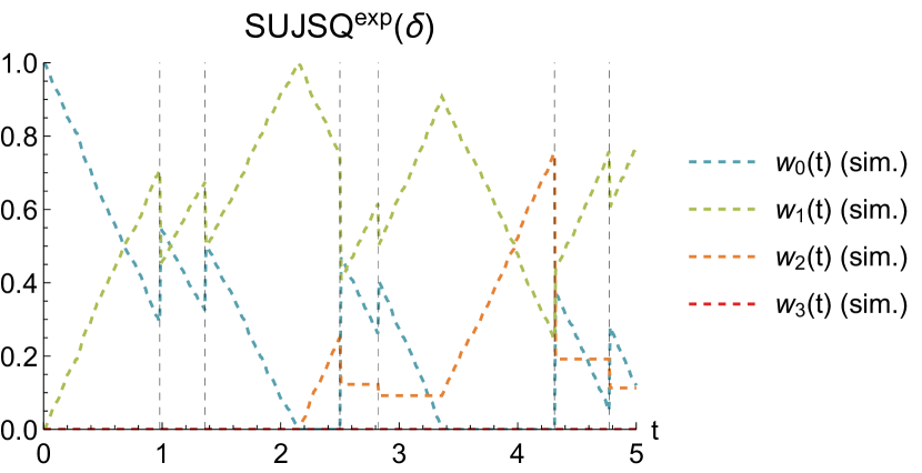
Figure 11. Simulation results for SUJSQ${}^{exp}(0.85)$.

Appendix F Simulation results for $\text{AUJSQ}^{\textup{det}}(\delta)$

The next four figures provide the simulation plots for a system with $N=400$ servers and $\lambda=0.7$, averaged over 100 runs for $\text{AUJSQ}^{\textup{det}}(\delta)$ as referred to in Section 5.1.2.

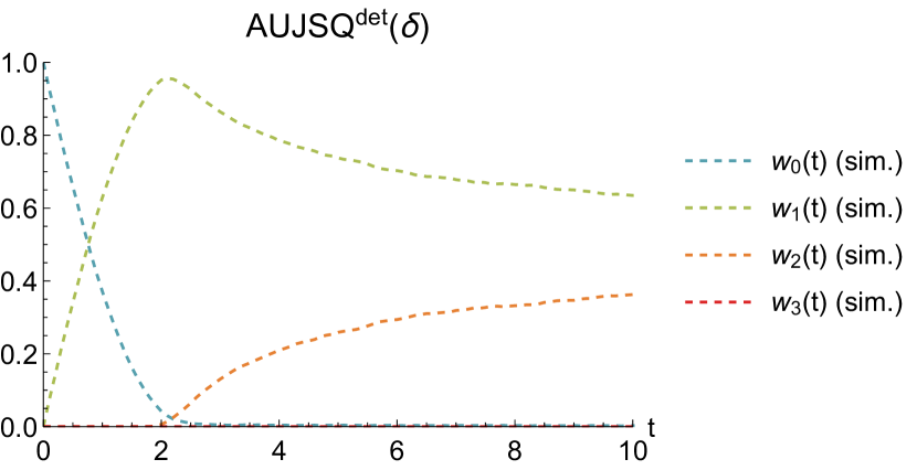
Figure 15. Simulation results for AUJSQ${}^{det}(0.85)$.

References

• (1)
• Alon et al. (2010) N Alon, O Gurel-Gurevich, and E Lubetzky. 2010. Choice-memory tradeoff in allocations. Ann. Appl. Probab. 20, 4 (08 2010), 1470–1511. https://doi.org/10.1214/09-AAP656
• Anselmi and Dufour (2018) J Anselmi and F Dufour. 2018. Power-of-$d$-Choices with Memory: Fluid Limit and Optimality. arXiv preprint arXiv:1802.06566 (2018).
• Badonnel and Burgess (2008) R Badonnel and M Burgess. 2008. Dynamic pull-based load balancing for autonomic servers. In Network Operations and Management Symposium, 2008. NOMS 2008. IEEE. IEEE, 751–754.
• Bramson et al. (2010) M Bramson, Y Lu, and B Prabhakar. 2010. Randomized load balancing with general service time distributions. In ACM SIGMETRICS Performance Evaluation Review, Vol. 38(1). ACM, 275–286.
• Bramson et al. (2012) M Bramson, Y Lu, and B Prabhakar. 2012. Asymptotic independence of queues under randomized load balancing. Queueing Systems 71, 3 (2012), 247–292.
• Ephremides et al. (1980) A Ephremides, P Varaiya, and J Walrand. 1980. A simple dynamic routing problem. IEEE transactions on Automatic Control 25, 4 (1980), 690–693.
• Gamarnik et al. (2016) D Gamarnik, J N Tsitsiklis, and M Zubeldia. 2016. Delay, memory, and messaging tradeoffs in distributed service systems. ACM SIGMETRICS Performance Evaluation Review 44, 1 (2016), 1–12.
• Gandhi et al. (2014) R Gandhi, H H Liu, Y C Hu, G Lu, J Padhye, L Yuan, and M Zhang. 2014. Duet: Cloud scale load balancing with hardware and software. ACM SIGCOMM Computer Communication Review 44, 4 (2014), 27–38.
• Gast (2017) N Gast. 2017. Expected values estimated via mean-field approximation are 1/N-accurate. Proceedings of the ACM on Measurement and Analysis of Computing Systems 1, 1 (2017), 17.
• Gupta and Walton (2019) V Gupta and N Walton. 2019. Load Balancing in the Nondegenerate Slowdown Regime. Operations Research (2019).
• Hunt and Kurtz (1994) P J Hunt and T G Kurtz. 1994. Large loss networks. Stochastic Processes and their Applications 53, 2 (1994), 363–378.
• Lu et al. (2011) Y Lu, Q Xie, G Kliot, A Geller, J R Larus, and A Greenberg. 2011. Join-Idle-Queue: A novel load balancing algorithm for dynamically scalable web services. Performance Evaluation 68, 11 (2011), 1056–1071.
• Luczak and Norris (2013) M J Luczak and J R Norris. 2013. Averaging over fast variables in the fluid limit for Markov chains: application to the supermarket model with memory. The Annals of Applied Probability 23, 3 (2013), 957–986.
• Maguluri et al. (2012) S T Maguluri, R Srikant, and L Ying. 2012. Stochastic models of load balancing and scheduling in cloud computing clusters. In INFOCOM, 2012 Proceedings IEEE. IEEE, 702–710.
• Mitzenmacher (2000) M Mitzenmacher. 2000. How useful is old information? IEEE Transactions on Parallel and Distributed Systems 11, 1 (2000), 6–20.
• Mitzenmacher (2001) M Mitzenmacher. 2001. The power of two choices in randomized load balancing. IEEE Transactions on Parallel and Distributed Systems 12, 10 (2001), 1094–1104.
• Mitzenmacher et al. (2002) M Mitzenmacher, B Prabhakar, and D Shah. 2002. Load balancing with memory. In The 43rd Annual IEEE Symposium on Foundations of Computer Science, 2002. Proceedings. 799–808. https://doi.org/10.1109/SFCS.2002.1182005
• Mukherjee et al. (2016) D Mukherjee, S C Borst, J SH Van Leeuwaarden, and P A Whiting. 2016. Universality of load balancing schemes on the diffusion scale. Journal of Applied Probability 53, 4 (2016), 1111–1124.
• Mukhopadhyay et al. (2016) A Mukhopadhyay, A Karthik, and R R Mazumdar. 2016. Randomized assignment of jobs to servers in heterogeneous clusters of shared servers for low delay. Stochastic Systems 6, 1 (2016), 90–131.
• Mukhopadhyay et al. (2015) A Mukhopadhyay, A Karthik, R R Mazumdar, and F Guillemin. 2015. Mean field and propagation of chaos in multi-class heterogeneous loss models. Performance Evaluation 91 (2015), 117–131.
• Mukhopadhyay and Mazumdar (2014) A Mukhopadhyay and R R Mazumdar. 2014. Randomized routing schemes for large processor sharing systems with multiple service rates. In ACM SIGMETRICS Performance Evaluation Review, Vol. 42(1). ACM, 555–556.
• Pang et al. (2007) G Pang, R Talreja, and W Whitt. 2007. Martingale proofs of many-server heavy-traffic limits for Markovian queues. Probability Surveys 4 (2007), 193–267.
• Patel et al. (2013) P Patel, D Bansal, L Yuan, A Murthy, A Greenberg, D A Maltz, R Kern, H Kumar, M Zikos, H Wu, K Changhoon, and N Karri. 2013. Ananta: Cloud scale load balancing. ACM SIGCOMM Computer Communication Review 43, 4 (2013), 207–218.
• Stolyar (2015) A L Stolyar. 2015. Pull-based load distribution in large-scale heterogeneous service systems. Queueing Systems 80, 4 (2015), 341–361.
• Tsitsiklis and Xu (2012) J N Tsitsiklis and K Xu. 2012. On the power of (even a little) resource pooling. Stochastic Systems 2, 1 (2012), 1–66.
• Tsitsiklis and Xu (2013) J N Tsitsiklis and K Xu. 2013. Queueing system topologies with limited flexibility. In ACM SIGMETRICS Performance Evaluation Review, Vol. 41(1). ACM, 167–178.
• Vvedenskaya et al. (1996) N D Vvedenskaya, R L Dobrushin, and F I Karpelevich. 1996. Queueing system with selection of the shortest of two queues: An asymptotic approach. Problemy Peredachi Informatsii 32, 1 (1996), 20–34.
• Winston (1977) W Winston. 1977. Optimality of the shortest line discipline. Journal of Applied Probability 14, 1 (1977), 181–189.
• Xie et al. (2015) Q Xie, X Dong, Y Lu, and R Srikant. 2015. Power of d choices for large-scale bin packing: A loss model. ACM SIGMETRICS Performance Evaluation Review 43, 1 (2015), 321–334.
• Ying (2016) L Ying. 2016. On the approximation error of mean-field models. In ACM SIGMETRICS Performance Evaluation Review, Vol. 44(1). ACM, 285–297.
• Ying et al. (2015) L Ying, R Srikant, and X Kang. 2015. The power of slightly more than one sample in randomized load balancing. In Computer Communications (INFOCOM), 2015 IEEE Conference on. IEEE, 1131–1139.