Global Delocalization Transition in the de Moura-Lyra Model

Abstract

The possibility of having a delocalization transition in the 1D de Moura-Lyra class of models (having a power-spectrum $\propto q^{-\alpha}$) has been the object of a long standing discussion in the literature. In this paper, we report the first numerical evidences that such a transition happens at $\alpha=1$, where the localization length (measured from the scaling of the conductance) is shown to diverge as $(1-\alpha)^{-1}$. The persistent finite-size scaling of the data is shown to be caused by a very slow convergence of the nearest-neighbor correlator to its infinite-size limit, and controlled by the choice of a proper scaling parameter. Our results for these models are consistent with a localization of eigenstates that is driven by a persistent small-scale noise, which vanishes as $\alpha\to 1^{-}$. This interpretation in confirmed by analytical perturbative calculations which are built on previous work. Finally, the nature of the delocalization transition is discussed and the conclusions are illustrated by numerical work done in the $\alpha>1$ regime.

I Introduction

It is an established fact that all eigenstates of an one-dimensional hamiltonian usually become exponentially localized in the presence of a random potential (Mott and Twose, 1961). Physically, this feature translates into a peculiar behavior of the system’s transport properties. Namely, the typical ($T=0K$) conductance over a disorder ensemble scales exponentially to zero as the length is increased, i.e. $G_{\text{Typ}}\propto\exp\left(-\nicefrac{{L}}{{\xi}}\right)$. (Lee and Ramakrishnan, 1985; Izrailev et al., 2012) The characteristic parameter $\xi$ is called the localization length and can be related to the characteristic size of the system’s eigenwavefunctions or, equivalently, to the real-space decay length of the single-particle Green’s function. (Thouless, 1972)

For one-dimensional models with uncorrelated disorder, the existence of localized states at all energies was settled long ago, both by rigorous analytical methods (Ziman, 1968; Ishii, 1973) and numerical simulations (Andereck and Abrahams, 1980; Pichard, 1986). On the contrary, the role played by space-correlations in the disordered potential remains unclear. The early attempts to deal with correlated disorder models (Johnston and Kramer, 1986) did not show any qualitative differences in the physics of the system, other than by changing the specific values of the localization length. Later on, more sophisticated models were invented in which the existence of delocalized eigenstates was revealed. An important example is the so called random dimer model (and its generalizations (Dunlap et al., 1990; Phillips and Wu, 1991)), where the random placement of different dimers across a chain generates delocalized states at isolated energies.

Despite having extended states, models like the ones described above do not give rise to true mobility edges in the thermodynamic limit. The first evidence that such a feature could appear in 1D stemmed from the study of self-affine potentials pioneered by de Moura and Lyra (de Moura and Lyra, 1998). They defined a random potential with a power-spectrum decaying as $q^{-\alpha}$, which is known to occur naturally in the assembly of biological macromolecules, such as DNA(Peng et al., 1992). For $\alpha\approx 0,$ one recovers the fully localized uncorrelated model, while in the opposite limit ($\alpha\rightarrow+\infty$) the potential becomes ordered and there is a complete delocalization. By numerically studying the Lyapunov exponent as a function of $\alpha$, de Moura and Lyra concluded that an Anderson transition happens at $\alpha=2$, followed by the emergence of a mobility edge in the spectrum. These results were contested (Kantelhardt et al., 2000) on the basis of the ill-defined thermodynamic limit in these potentials. Eventually, it was understood that the presumed transition is an artifact of the anomalous scaling of the Lyapunov exponent, due to the non-stationarity of the potential for any $\alpha\geq 1$. (Russ et al., 2001; Bunde et al., 2000) This reasoning was reexamined some years later by G. M. Petersen et al (Petersen and Sandler, 2013), who reaffirmed the appearance of a mobility edge at $\alpha=2$ and connected it to the increasing infinite-range anticorrelations of the disordered potential.

Despite the current knowledge about the non-stationary sector of the de Moura-Lyra model, little attention has been given to the cases when $\alpha\in\left[0,1\right[$. The purpose of this paper is to fill this gap by studying the behavior of the localization length as $\alpha\rightarrow 1^{-}$, where the model goes from a truly disordered stationary potential to a non-stationary one (where the states are conjectured to be extended). More precisely, we report the first clear observation of a delocalization phase transition, happening at $\alpha=1$ for all energies, without generating a mobility edge. Moreover, a detailed analysis of the disorder’s real-space correlations for $\alpha<1$ is done which, besides clarifying the origin of the persistent finite-size scaling in the measured localization length, also shows that the most relevant feature for the localization of the eigenstates is the magnitude of very short-scale disorder, rather than the power-law tails of the correlator. Anticipating the results, we state that our numerical and analytical definitely settle the issue in favor of the full delocalization for any $\alpha\geq 1$ and, at same time, clearly invalidates the use of the de Moura-Lyra model to study the effect of algebraic correlations in the disordered potential, even when it is stationary.

The remaining text is organized as follows: In sect. II, we recover the definition of the de Moura-Lyra disorder model, focusing on the calculation of its statistical properties in the thermodynamic limit, while showing the relevance of finite-size deviations close to the transition point; In Sect. III, we apply the generalized Thouless formula(Izrailev and Krokhin, 1999) to calculate perturbatively the localization length as a function of $\alpha$. In Sect. IV, the Landauer conductance of many disordered samples is numerically calculated, and the linear scaling of its typical value is used to determine the localization length for several values of $\alpha$. In Sect. V, the finite size scaling of the localization length is analyzed and a perfect collapse of the data is accomplished in the perturbative regime. In Sect. VI, we recap all the results and sum up our conclusions.

II Model and Disorder Statistics

The focus of this work is on the localization phenomena happening in nearest-neighbor tight-binding chains with an on-site disordered potential having long-ranged space correlations. The respective Hamiltonian is

$$\mathcal{H}=\sum_{n=0}^{L}\varepsilon_{n}c_{n}^{\dagger}c_{n}-\sum_{n=0}^{L-1}\left(c_{n}^{\dagger}c_{n+1}+c_{n+1}^{\dagger}c_{n}\right),$$ (1)

where $\varepsilon_{n}$ stands for on-site values of the disordered potential (in units of the hopping).

II.1 Disorder Statistics in the Thermodynamic Limit

In order to generate a correlated random potential, we employ the well-known Inverse Fourier Transform Method (IFTM) (de Moura and Lyra, 1998; Petersen and Sandler, 2013; Khan et al., 2019) meaning that the disorder profile is defined as the Fourier sum 

$$\varepsilon_{n}=\sum_{q\neq 0}V(q)e^{iqn+i\phi_{q}},$$ (2)

where $\phi_{q}$ are statistically independent random phases, obeying the reality constraint, $\phi_{q}=-\phi_{-q}$. For the present purposes, we are interested on the special case of the de Moura-Lyra potential, where $V(q)=\mathcal{A}\left(\alpha\right)\left|q\right|^{-\frac{\alpha}{2}}$, and focus on the $0\leq\alpha<1$ sector, in which the thermodynamic limit does not suffer from the mathematical pathologies of the $\alpha\geq 1$ cases (Petersen and Sandler, 2013; Khan et al., 2019).

By construction, the ensemble average of the on-site energies is zero, while the local variance is seen to be site-independent and equal to

$$\left\langle\varepsilon_{n}^{2}\right\rangle=2\mathcal{A}\left(\alpha\right)^{2}\sum_{q>0}q^{-\alpha}\xrightarrow[L\rightarrow\infty]{}\frac{L\mathcal{A}\left(\alpha\right)^{2}}{\pi^{\alpha}\left(1-\alpha\right)}.$$ (3)

By fixing the variance to $\sigma_{\varepsilon}^{2}$, we also fix the normalization constant to be $\mathcal{A}(\alpha)=\sigma_{\varepsilon}\sqrt{\left(1-\alpha\right)\pi^{\alpha}/L}$. Similarly, we may calculate the normalized two-point correlator of $\varepsilon_{n}$, which yields

$$\mathcal{C}_{\alpha}^{\infty}(r) =\frac{\left\langle\varepsilon_{n}\varepsilon_{n+r}\right\rangle}{\sigma_{\varepsilon}^{2}}=\frac{1-\alpha}{\pi^{1-\alpha}}\int_{0}^{\pi}\frac{\cos qr}{q^{\alpha}}dq$$ (4)

$$\qquad\qquad\qquad=\;_{1}F_{2}\left(\frac{1-\alpha}{2},\frac{1}{2},\frac{3-\alpha}{2},-\frac{\pi^{2}r^{2}}{4}\right).$$

Despite being a complicated Hypergeometric function, $\mathcal{C}_{\alpha}^{\infty}(r)$ has a rather simple asymptotic expansion in $r$ (i.e. with $1\ll r\ll L$), which shows the correlations falling-off as $r^{\alpha-1}$ , i.e.

$$\mathcal{C}_{\alpha}^{\infty}\left(r\right)=\frac{\Gamma\left(\frac{1-\alpha}{2}\right)}{\Gamma\left(\frac{\alpha}{2}\right)}\frac{\pi^{\alpha-\frac{1}{2}}\left(1-\alpha\right)}{2^{\alpha}r^{1-\alpha}}+\mathcal{O}\left(\frac{1}{r^{2}}\right).$$ (5)

The plot presented in Fig. 1 a) shows that this algebraic behavior sets in after only a few lattice spacings.

Other than the slow decay of the correlations at large distances, one also notices that there is a very sharp uncorrelation across a single bond. This features disappear as $L\rightarrow\infty$ and $\alpha\rightarrow 1^{-}$ (by this order), but for a finite system and $\alpha<1$ it is enough to generate a small-scale random noise with an amplitude of the order of $\sigma_{\varepsilon}$ (e.g. see Fig. 1 b)).

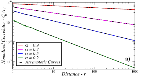
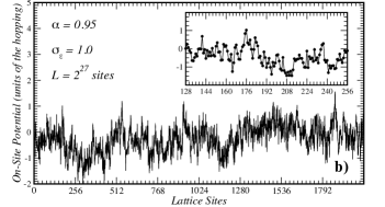
Figure 1: a) Plots of the normalized correlation function for the de Moura-Lyra model, in the limit $L\rightarrow+\infty$. The black dashed lines are the asymptotic expressions $\mathcal{C}_{\alpha}^{\infty}(r)\propto r^{\alpha-1}$; b) An example of the de Moura-Lyra disorder profile (including a zoom in the inset). (color online)

II.2 Finite Size Effects

In a finite sample of size $L$, an appropriate measure for the strength of this short-distance noise component is the (squared) Normalized Single-Bond Discontinuity (NSBD) parameter, defined as

$$\mathcal{D}_{\alpha}^{L}=\frac{\left\langle\left(\varepsilon_{n}-\varepsilon_{n+1}\right)^{2}\right\rangle}{2\sigma_{\varepsilon}^{2}}=1-\mathcal{C}_{\alpha}^{L}(1).$$ (6)

This parameter roughly measures the dispersion of on-site energies, relative to the previous value. In the $L\to\infty$ limit, by expanding the function of Eq. 4, this quantity is shown to be proportional to $(1-\alpha)$ in the limit $\alpha\to 1^{-}$. On the other hand, simulated finite systems have $L$-dependent space correlators given by

$$\mathcal{C}_{\alpha}^{L}(r)=\frac{\sum_{i=1}^{\nicefrac{{L}}{{2}}}i^{-\alpha}\cos\frac{2\pi ir}{L}}{\sum_{i=1}^{\nicefrac{{L}}{{2}}}i^{-\alpha}},$$ (7)

instead of Eq. 4.

In the Fig. 2, we compare the exact correlator and NSBD to the expression of Eq. 4 for different sample sizes, being quite evident the very slow convergence towards the thermodynamic limit value, especially for values of $\alpha$ close to $1$. This very slow convergence of the NSBD to its limiting value is shown to cause a persistent finite-size scaling of the calculated localization length. This is also the reason for the persistence of the small-scale noise, even when $\alpha$ is very close to $1$, as seen in Fig. 1 b).

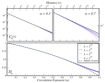
Figure 2: Examples of the finite-size effects on the correlator $\mathcal{C}_{\alpha}^{L}(r)$ (upper panels) and the NSBD parameter $\mathcal{D}_{\alpha}^{L}$ (lower panel). The dashed lines stand for the curves obtained in the thermodynamic limit ($L\to\infty$). (color online)

III Perturbative Expression for the Localization Length

In the weak disordered regime, one can usually obtain analytical expressions for the localization length, as a function of energy. In fact, F. M. Izrailev (Izrailev and Krokhin, 1999) derived a generalized Thouless formula which allows the calculation of $\xi$ for arbitrary space-correlated disordered potentials, in first order on the local variance $\sigma_{\varepsilon}^{2}$. In the thermodynamic limit, it reads:

$$\xi^{-1} =\frac{\sigma_{\varepsilon}^{2}}{8\sin^{2}\left(k\right)}\left\{1+2\sum_{r=1}^{\infty}\mathcal{C}_{\alpha}^{\infty}\left(r\right)\cos\left(2kr\right)\right\}$$ (8)

$$\qquad\qquad\qquad\qquad=\frac{\sigma_{\varepsilon}^{2}}{8\sin^{2}\left(k\right)}\sum_{r=-\infty}^{\infty}\mathcal{C}_{\alpha}^{\infty}\left(r\right)e^{i2kr},$$

where $k=\arccos\left(E/2\right)$ is the (positive) wavenumber associated to an unperturbed band energy $E$. In order to apply Eq. 8 to our disorder model, we must plug in the correlator of Eq. 4, yielding

$$\xi^{-1} =\frac{\pi^{\alpha-1}\sigma_{\varepsilon}^{2}}{16\sin^{2}\left(k\right)}\left(1-\alpha\right)\int_{-\pi}^{\pi}\sum_{r=-\infty}^{\infty}\frac{e^{i\left(2k-q\right)r}}{\left|q\right|^{\alpha}}dq$$ (9)

$$\qquad\qquad\qquad\qquad\qquad\qquad=\frac{\pi^{\alpha}\sigma_{\varepsilon}^{2}}{8\sin^{2}\left(k\right)}\frac{\left(1-\alpha\right)}{\left|2k\right|^{\alpha}}.$$

Finally, if we express it in terms of the energy, we get to the final expression:

$$\xi=\frac{2}{\left(1-\alpha\right)\sigma_{\varepsilon}^{2}}\left(4-E^{2}\right)\left[\frac{2}{\pi}\arccos\left(\frac{E}{2}\right)\right]^{\alpha}.$$ (10)

From Eq. 10 it is evident that for any value of the band energy, the localization length is finite. However, as $\alpha\rightarrow 1^{-}$ this length diverges as $\left(1-\alpha\right)^{-1}$, signaling the existence of a global delocalization transition at that point, i.e without generating any mobility edge.

IV Localization Length From the Landauer Conductance

The existence of a finite localization length $\xi$ leads to a quantum conductance which has a self-averaging log-normal statistics over the ensemble and a typical value that scales exponentially to zero with $\nicefrac{{L}}{{\xi}}$. Hence, in order to measure it, we made use of the linearized Landauer Formula (Landauer, 1970; Caroli et al., 1971; Meir and Wingreen, 1992; Wimmer, 2009) for the conductance (of a two-terminal device):

$$G\left(E_{F}\right)=\frac{e^{2}}{h}\left(4-E_{F}^{2}\right)\left|\mathcal{G}_{L_{S}+1,0}^{r}(E_{F})\right|^{2},$$ (11)

where $L_{S}$ is the number of sites in the sample, $E_{F}$ is the Fermi energy and $\mathcal{G}^{r}$ stands for the retarded real-space Green’s function. For a given sample of disorder, the latter may be calculated using the Recursive Green Function Method (MacKinnon, 1985) with the exact surface Green’s functions of the leads as boundary conditions.

In all our calculations, we considered the disordered samples to be different sized pieces (subchains of size $L_{S}$) cut from independently generated potentials with $L_{\text{Tot}}$ sites. Then, $L_{\text{Tot}}$ was increased in order to approach the thermodynamic limit of the disorder statistics. In Fig. 3 a), we illustrate the results with an example, from where the referred features of localization are very evident. This same procedure was then repeated for different values of $\alpha$, $\sigma_{\varepsilon}$ and $L_{\text{Tot}}$, and the localization length was obtained from the inverse slope of a linear fit to the $\left\langle\log\left(\frac{h}{e^{2}}G\right)\right\rangle$ as function of $L_{S}$. Some of those results are presented in Fig. 3 b).

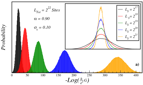
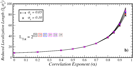
Figure 3: a) Example of the histograms obtained for the $\log\left(\frac{h}{e^{2}}G\right)$ of subchains drawn from $10^{5}$ (independent) disordered samples with $L_{\text{Tot}}=2^{22}$ sites, $\sigma_{\varepsilon}=0.1$ and $\alpha=0.90$. In the inset, we have the same histograms rescaled by corresponding subchain size, making clear that this quantity is self-averaging and with an average which scales linearly with $L_{S}$. b) Plot of the localization length as a function of $\alpha$ for different values of $L_{\text{Tot}}$ (notice the color code). (color online)

V Finite-Size Scaling And Critical Behavior of The Localization Length

V.1 Results and Interpretation

From Fig. 3 b) the localization length is seen to increase with $\alpha$. Nevertheless, it is not evident that it is diverging as predicted by Eq. 10., due to the persistent finite-size scaling present in the data for high values of $\alpha$.

This scaling of the localization length is driven by the slow convergence of the disorder statistics to its thermodynamic limit. In particular, as referred in Sect. IIB, even for values of $\alpha$ very close to the transition point there is a sizable random noise at small distances, whose amplitude goes very slowly to zero as $L_{\text{Tot}}$ is increased. Our central argument in this paper is that the main contribution to the eigenstates’ localization comes from this small-scale component, which has an effective strength measured by $\sqrt{\mathcal{D}_{\alpha}^{L_{\text{Tot}}}}$. The latter claim can be proven by plotting the data in Fig. 3 b) as a function of this parameter, instead of $\alpha$. This is done in Fig. 4 a), and a perfect collapse of all the points is obtained for small enough values of $\sigma_{\varepsilon}$.

The great advantage of this new representation is that we accomplish a complete control over the finite-size scaling phenomenon: with increasing in $L_{\text{Tot}}$, all the points slide over the dashed curve, slowly approaching a fixed value. In other words, we turned a two-parameter scaling, $\sigma_{\varepsilon}^{2}\xi=f_{1}\left(L_{Tot},\alpha\right)$, into a single-parameter scaling, $\sigma_{\varepsilon}^{2}\xi=f_{2}\left(\mathcal{D}_{\alpha}^{L_{Tot}}\right)$. This scaling law was used to extrapolate the values of $\xi$ to the thermodynamic limit, with the following procedure:

1. Calculate the thermodynamic limit values of $\mathcal{D}_{\alpha}^{\infty}=\lim_{L_{Tot}\to\infty}\left(\mathcal{D}_{\alpha}^{L_{Tot}}\right)$ from the Eqs. 4 and 6, for each value of $\alpha$;

2. Use the finite-size scaling curves (dashed curves in Fig. 4 b)) to read the values the thermodynamic limit of $\xi(\alpha)$;

3. Plot the corresponding values as a function of $\alpha$ and compare them with the analytical expression of Eq. 10.

The final results are shown in Fig. 4 c) , where it is clear that we have a perfect agreement with the analytical results of Sect. III. For completeness, we also checked this behavior for different energies, which yielded a similar collapse of the data (see Fig. 4 b)) and agreement with Eq. 10, thus confirming the belief that this transition occurs over all the spectrum at once. A direct fit of the data points in Fig. 4 c) , to a function of the form $\xi\left(\alpha\right)=C\left(\alpha_{C}-\alpha\right)^{-\nu}$ yields the following results:

• For $E_{F}=0.0$:

  • $\alpha_{C}=1.0018\pm 0.0064$;

  • $\nu=1.032\pm 0.068$;

• For $E_{F}=0.5$:

  • $\alpha_{C}=0.9970\pm 0.0073$;

  • $\nu=0.953\pm 0.075$;

which are in numerical agreement with the analytical expression.

V.2 Delocalization or Insulator-Metal Transition?

Before closing this section, it is imperative to make some further comments on the physical interpretation of this divergence in $\xi$. More precisely: Does this divergence signal a transition from an insulating to a metallic phase?

A first concern shall be raised about the applicability of our procedure of cutting subchains from a larger sample and study their conductance, when $\alpha\geq 1$. Being non-stationary, the thermodynamic limit correlator $\mathcal{C}_{\alpha}^{\infty}$ is a function of $\nicefrac{{r}}{{L}}_{Tot}$ (see Refs.(Petersen and Sandler, 2013; Khan et al., 2019)) and not simply of $r$, as in Eq. 4. One consequence of this is the following: If we take a fixed sized subchain from increasingly larger chains, the values of $\varepsilon_{n}$ in the subchains will become more and more correlated and, in the limit $L_{Tot}\to\infty$, they will form an uniform potential inside the subchain. Hence, any finite subchain will be ordered in this limit and therefore metallic. Additionally, this argument invalidates immediately the existence of a finite localization length for any $\alpha\geq 1$.

However, one could have used subchains whose size is a fixed fraction of $L_{Tot}$, i.e. $\gamma\equiv\nicefrac{{L_{S}}}{{L_{Tot}}}=\text{const}$. In such a case, the reasoning of last paragraph is no longer valid, but are the subchains still metallic? To answer this, we must remark that in an insulator-to-metal transition, one has a diverging $\xi$, but also a linear scaling of $\xi$ with the system size in the metallic phase. As is known from previous work(Russ et al., 2001; Bunde et al., 2000), the scaling of the localization length with the total system size is anomalous(Bunde et al., 2000) for any $\alpha>1$, i.e. $\xi\propto L_{Tot}^{\alpha-1}$. An implication of this result is that the scaling of $\left\langle\log\frac{h}{e^{2}}G\right\rangle$ is given by a function $f\left(\gamma,L_{Tot},\alpha\right)$, with the following form:

$$f\left(\gamma,L_{Tot},\alpha\right) =-\log\left[C_{1}\left(\alpha\right)\right]+\frac{L_{S}}{\xi\left(\alpha,L_{tot}\right)}$$ (12)

$$\qquad=-\log\left[C_{1}\left(\alpha\right)\right]+C_{2}\left(\alpha\right)\gamma L_{Tot}^{2-\alpha}.$$

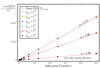
Figure 5: Plots of the $\left\langle\log\frac{hG}{e^{2}C_{1}\left(\alpha\right)}\right\rangle$ as a function of the fraction chain used, $\gamma=L_{s}/L_{Tot}$, for three values of $\alpha$ above the critical point. The $L_{Tot}$ dependence of the function $f(\gamma,L_{Tot,\alpha})$ in Eq. 12 was used to collapse the data for different different system sizes into a single straight line (dashed red lines). The value of the local variance used was $\sigma_{\varepsilon}=0.2$.

For a start, Eq. 12 makes clear that for any $\alpha>2$, the $\left\langle\log\frac{h}{e^{2}}G\right\rangle$ converges to the finite value $\log\left[C_{1}\left(\alpha\right)\right]$, in the limit $L_{Tot}\to\infty$ with $\gamma$ kept fixed. On the other hand, for $1\leq\alpha<2$ the situation is rather different, as it is the second term of Eq. 12 that dominates in that same limit. Thus, the system becomes an insulator as $L_{Tot}\to\infty$, as long as we take it with $\gamma$ fixed. Both these facts explain the originally observed(de Moura and Lyra, 1998) critical point at $\alpha=2$. At any rate, the scaling of Eq. 12 may also be checked by calculations analogous to the ones we made for $\alpha<1$. Our numerical results are shown in Fig. 5, where we show the data of $\left\langle\log\frac{h}{e^{2}}G\right\rangle\left(\gamma\right)$ for $6$ values of $L_{Tot}$ can be collapsed into a linear curve after subtracting $C_{1}\left(\alpha\right)$ (obtained by fitting) and rescaling by $L_{Tot}^{2-\alpha}$. This corroborates the validity of Eq. 12 for $\alpha\geq 1$.

Summarizing, the behavior of this model for $\alpha\to 1^{+}$ is a highly non-trivial one and, in particular, deciding whether or not the phase is metallic is dependent on the way the thermodynamic limit is taken. Therefore, what we mean by delocalization in the title of this paper is to be understood as the emergence of a phase without a well-defined finite length scale $\xi$.

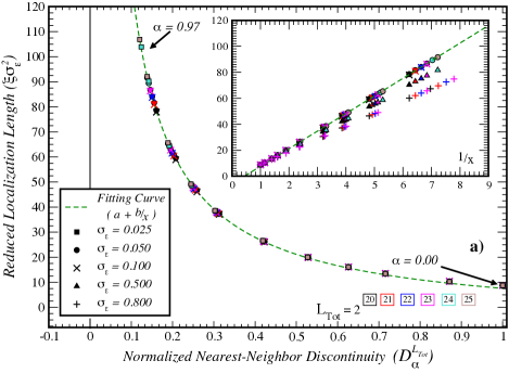
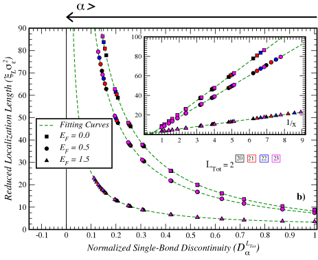
Figure 4: a) Plot of the localization length as a function of the NSBD for different values $\sigma_{\varepsilon}$. The green dashed curve corresponds to a fit for values close to $\mathcal{D}_{\alpha}^{L_{Tot}}=0$ of the sets with $\sigma_{\varepsilon}=0.025$, $0.05$ and $0.10$. The data for $\sigma_{\varepsilon}=0.5$ and $0.8$ (only in the inset) already show a deviation from this curve due to the breakdown of perturbation theory. b) Plot of the localization length as a function of the NSBD for different values of the energy and $\sigma_{\varepsilon}=0.10$. All three cases can be collapsed into curves of the type $y=a+\frac{b}{x}$, shown as dashed green lines. The data is linearized by the transformation $x\to\nicefrac{{1}}{{x}}$, in the insets. c) Comparison between the thermodynamic limit values of $\xi$ predicted by the dashed curves in b), with the plots of the analytical expression of Eq. 10. (color online)

VI Summary and Conclusions

In the previous sections, we discussed the problem of localization in a correlated disordered potential, with a power-spectrum $\propto q^{-\alpha}$. This model is known to have an ill-defined thermodynamic limit for $\alpha\geq 1$ (non-stationarity), but is perfectly well-defined for $\alpha\in\left[0,1\right[$, having correlations decaying as $r^{\alpha-1}$ for long distances and a significant uncorrelation across a single bond. This last feature generates a random noise at short distances with an effective strength given by the NSBD parameter — $\sqrt{\mathcal{D}_{\alpha}^{L_{Tot}}}$. The finite-size effects on the statistics of the disorder were also discussed and shown to be very relevant near $\alpha=1$.

Furthermore, by applying a generalized Thouless Formula due to F. M. Izrailev (Izrailev and Krokhin, 1999), we concluded that the localization length in this system is expected to diverge as $\left(1-\alpha\right)^{-1}$ for $\alpha\rightarrow 1^{-}$, at all points in the spectrum. These results were confirmed by a direct measurement of the localization length from the linear scaling of the typical Landauer conductance, which was shown to suffer from a persistent finite-size scaling near the transition point. This scaling was then related to the referred finite-size effects in the statistics and the NSBD was found to be the relevant parameter for studying it. By using the latter as a scaling parameter for the localization length, we were able to collapse all the data points into an universal curve, in the limit of small $\sigma_{\varepsilon}$. With this picture, the finite-size scaling appear as a “slide” of the points along that curve, approaching their thermodynamic limit value for each $\alpha$. Finally, the limiting curve was shown to be consistent with the result from Izrailev’s formula, and the existence of a global delocalization transition at $\alpha=1$.

To finish, we summarize our main conclusions in two two points:

1. We were able to numerically observe the existence of a delocalization transition in these models, at $\alpha=1$, and show that it agrees with analytical results in the weak-disordered regime. To the best of our knowledge, this is a novelty in the literature, which settles the matter in favor of an expected global delocalization of the eigenstates for $\alpha\geq 1$;

2. The way we were able to control the finite-size scaling of the localization length provides us with very clear evidences about the true nature of the said transition. As a matter of fact, the observed behavior of $\xi\left(\mathcal{D}_{\alpha}^{L_{Tot}}\right)$ in the perturbative regime is exactly the same as one would expect from an uncorrelated Anderson disorder, with an effective strength given by $\sqrt{\mathcal{D}_{\alpha}^{L_{Tot}}}.$ This fact gives a strong indication that the variation of the localization length with the exponent $\alpha$ is mainly due to a varying effective strength of the short-scale noise, and not due to the change in the tail’s exponent of the real-space disorder correlator. Nonetheless, the two effects cannot be decoupled in the de Moura-Lyra model as there is there is a single parameter, $\alpha$, controlling both the vanishing of the local noise component and the power-law tail’s exponent.

In our perspective, both points are equally relevant for the physical interpretation of this disorder model, in the sense that both lead to a final conclusion: the model is as unable to generate 1D Anderson transitions (for which it was built), as it is of reproducing the effects power-law tails in the real-space disorder correlator. In fact, the localization phenomena seems to be as simple here, as in an uncorrelated Anderson model and the delocalization transition is a disorder-to-order one. An interesting follow-up to the present work would be finding new ways of simulating stationary disorder landscapes having power-law tails with tunable exponents but a possibly negligible and independently determined small-scale noise. Analyzing systems with such potentials would give us information about the importance of algebraic correlation tails in the physics of one-dimensional localization.

VII Acknowledgments

We thank the helpful comments and suggestions of the Physical Review B referees, which contributed to the improvement of this work.

For this work, J. P. Santos Pires was supported by the MAP-fis PhD grant PD/BD/142774/2018 of Fundação da Ciência e Tecnologia; N. A. Khan was supported by the grants ERASMUS MUNDUS Action 2 Strand 1 Lot 11, EACEA/42/11 Grant Agreement 2013-2538 / 001-001 EM Action 2 Partnership Asia-Europe and the research scholarship UID/FIS/04650/2013 of Fundação da Ciência e Tecnologia. The authors also acknowledge financing from Fundação da Ciência e Tecnologia and COMPETE 2020 program in FEDER component (European Union), through the projects POCI-01-0145-FEDER-02888 and UID/FIS/04650/2013.

References

- Mott and Twose (1961) N. Mott and W. Twose, Adv. Phys. 10, 107 (1961).
- Lee and Ramakrishnan (1985) P. A. Lee and T. V. Ramakrishnan, Rev. Mod. Phys. 57, 287 (1985).
- Izrailev et al. (2012) F. M. Izrailev, A. A. Krokhin, and N. M. Makarov, Phys. Rep. 512, 125 (2012).
- Thouless (1972) D. J. Thouless, J. Phys. C: Sol. St. Phys. 5, 77 (1972).
- Ziman (1968) J. M. Ziman, J. Phys. C: Sol. St. Phys. 1, 1532 (1968).
- Ishii (1973) K. Ishii, Prog. Theor. Phys. Supp. 53, 77 (1973).
- Andereck and Abrahams (1980) B. S. Andereck and E. Abrahams, J. Phys. C: Sol. St. Phys. 13, L383 (1980).
- Pichard (1986) J. L. Pichard, J. Phys. C: Sol. St. Phys. 19, 1519 (1986).
- Johnston and Kramer (1986) R. Johnston and B. Kramer, Z. Phys. B: Cond. Matt. 63, 273 (1986).
- Dunlap et al. (1990) D. H. Dunlap, H.-L. Wu, and P. W. Phillips, Phys. Rev. Lett. 65, 88 (1990).
- Phillips and Wu (1991) P. W. Phillips and H.-L. Wu, Science 252, 1805 (1991).
- de Moura and Lyra (1998) F. A. B. F. de Moura and M. L. Lyra, Phys. Rev. Lett. 81, 3735 (1998).
- Peng et al. (1992) C. K. Peng, S. V. Buldyrev, A. L. Goldberger, S. Havlin, F. Sciortino, M. Simons, and H. E. Stanley, Nature 356, 168 (1992).
- Kantelhardt et al. (2000) J. W. Kantelhardt, S. Russ, A. Bunde, S. Havlin, and I. Webman, Phys. Rev. Lett. 84, 198 (2000).
- Russ et al. (2001) S. Russ, J. W. Kantelhardt, A. Bunde, and S. Havlin, Phys. Rev. B 64, 134209 (2001).
- Bunde et al. (2000) A. Bunde, S. Havlin, J. Kantelhardt, S. Russ, and I. Webman, Jour. Mol. Liq. 86, 151 (2000).
- Petersen and Sandler (2013) G. M. Petersen and N. Sandler, Phys. Rev. B 87, 195443 (2013).
- Izrailev and Krokhin (1999) F. M. Izrailev and A. A. Krokhin, Phys. Rev. Lett. 82, 4062 (1999).
- Khan et al. (2019) N. A. Khan, J. M. V. P. Lopes, J. P. dos Santos Pires, and J. M. B. L. dos Santos, J. Phys.: Condens. Matter 31, 175501 (2019).
- Note (1) The mode is an uniform potential contribution which may always be neglected. All the summations over in this paper are to be understood as summations over the allowed wavenumbers inside the First Brillouin Zone of an one-dimensional periodic chain, i.e. with .
- Note (2) The limit is somewhat special, since for any , recovering the usual uncorrelated Anderson disorder.
- Landauer (1970) R. Landauer, Phil. Mag. 21, 863 (1970).
- Caroli et al. (1971) C. Caroli, R. Combescot, P. Nozieres, and D. Saint-James, J. Phys. C: Sol. St. Phys. 4, 916 (1971).
- Meir and Wingreen (1992) Y. Meir and N. S. Wingreen, Phys. Rev. Lett. 68, 2512 (1992).
- Wimmer (2009) M. Wimmer, Quantum transport in nanostructures: from computational concepts to spintronics in graphene and magnetic tunnel junctions, Ph.D. thesis, Univ.-Verl. Regensburg (2009), OCLC: 551979435.
- MacKinnon (1985) A. MacKinnon, Z. Phys. B: Cond. Matt. 59, 385 (1985).
- Note (3) The data set for do not have enough points close to the singularity to provide a good estimate of .