Generalized Fast-Convolution-based Filtered-OFDM: Techniques and Application to 5G New Radio

Generalized Fast-Convolution-based Filtered-OFDM: Techniques and Application to 5G New Radio

Abstract

This paper proposes a generalized model and methods for fast-convolution (FC)-based waveform generation and processing with specific applications to fifth generation new radio (5G-NR). Following the progress of 5G-NR standardization in 3rd generation partnership project (3GPP), the main focus is on subband-filtered cyclic prefix (CP) orthogonal frequency-division multiplexing (OFDM) processing with specific emphasis on spectrally well localized transmitter processing. Subband filtering is able to suppress the interference leakage between adjacent subbands, thus supporting different numerologies for so-called bandwidth parts as well as asynchronous multiple access. The proposed generalized FC scheme effectively combines overlapped block processing with time- and frequency-domain windowing to provide highly selective subband filtering with very low intrinsic interference level. Jointly optimized multi-window designs with different allocation sizes and design parameters are compared in terms of interference levels and implementation complexity. The proposed methods are shown to clearly outperform the existing state-of-the-art windowing and filtering-based methods.

I Introduction

Orthogonal frequency-division multiplexing (OFDM) is the dominating multicarrier modulation scheme, being extensively deployed in modern radio access systems. OFDM offers high flexibility and efficiency in allocating spectral resources to different users, simple and robust way of channel equalization due to the inclusion of cyclic prefix (CP), as well as simplicity of combining multi-antenna schemes with the core physical layer processing [1]. The main drawback is the limited spectrum localization, especially, in challenging new spectrum use scenarios, like asynchronous multiple access, as well as mixed-numerology cases aiming to use adjustable symbol and CP lengths, subcarrier spacings, and frame structures depending on the service requirements [2, 3].

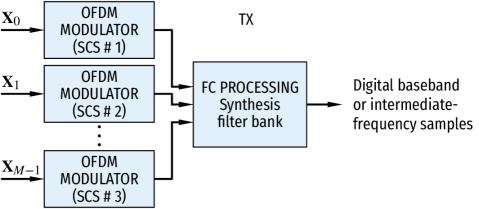
Figure 1: In fast-convolution (FC)-based filtered-OFDM, filtering is applied at subband level, which means one or multiple contiguous physical resource blocks (PRBs) with same subcarrier spacing (SCS), while utilizing normal CP-OFDM waveform for the PRBs. Transmitter processing uses FC synthesis filter bank for combining $M$ subbands.

In the emerging fifth generation new radio (5G-NR) mobile networks, building on orthogonal frequency-division multiple access (OFDMA) based radio interface, the ability to control the spectral characteristics of the transmitted waveform and receiver filtering, either over the whole carrier or over the so-called bandwidth parts [4] or subbands, is of particular importance. This is primarily due to the requirements to increase the bandwidth utilization, in the form of wider passband for given channel bandwidth, and to support efficient multiplexing of different services with different radio interface numerologies within a carrier. An important concrete example is the frequency multiplexing of enhanced mobile broadband (eMBB) and ultra-reliable low-latency communications (URLLC) services within the same NR carrier, with different SCSs (e.g., $15\text{\,}\mathrm{k}\mathrm{H}\mathrm{z}$, $30\text{\,}\mathrm{k}\mathrm{H}\mathrm{z}$, and $60\text{\,}\mathrm{k}\mathrm{H}\mathrm{z}$) as illustrated in Fig. 1. Such multiplexed signals with different SCSs are not orthogonal, calling for enhanced spectral localization of the signals to minimize interference while allowing high spectral efficiency and flexibility.

Additionally, it is important to acknowledge that the new radio (NR) specifications [4, and references therein] do not explicitly state how such spectral enhancements are implemented, and that the spectral enhancement methods used in transmitters must be transparent to receivers (and vice versa) [5]. The fundamental definition of transparent waveform processing means that the more advanced TX and RX solutions have to work with basic CP-OFDM RX or TX, respectively [6]. For this reason, in this article, the reference RX assumed in the optimization of the transmitter side signal processing methods is a basic cyclic prefix orthogonal frequency-division multiplexing (CP-OFDM) RX, while the use of more advanced RX schemes is then considered in the numerical radio link performance evaluations. It is also noted that transparent operation does not require completely error or distortion free signal quality with different TX-RX combinations but that the quality fulfills the requirements set by the considered technology and standard [5].

In general, there are multiple alternative solutions in the existing literature to improve the spectral characteristics of CP-OFDM systems [7, 8, 9, 10, 11, 12]. Time-domain windowing combined with overlap-and-add processing, commonly referred to as windowed overlap-and-add (WOLA), is a computationally inexpensive method to improve the spectral containment to a certain extent [7, 11]. The non-rectangular window with smooth transitions require either the extension of the symbol duration, reducing the spectral efficiency, or using part of the CP, resulting to a reduced tolerance to time dispersion [10]. Time-domain convolution based filtered OFDM (f-OFDM) or universal filtered OFDM (UF-OFDM), in general, require high-order filters with high complexity to achieve good frequency selectivity with narrow transition bands[8, 9, 13]. The complexity can be reduced by using polyphase filter-bank approaches, like [14], however, in this case the subbands typically have the same bandwidths and thus the configurability is impaired.

In transform-based fast-convolution (FC) filtering solutions, time-domain (TD) convolution is realized through element-wise multiplication (windowing) of frequency-domain (FD) sequences. This approach provides very high flexibility since the subband frequency response can be directly determined using the FD window values, allowing arbitrary bandwidths and center frequencies for the subbands. In our earlier works [15, 16, 13], we have developed FC-based processing solutions for efficient and flexible implementation of filtered OFDM physical layer in 5G-NR. In [13], the complexity and the performance of the FC processing are also compared with WOLA and other filtered-OFDM schemes.

In this article, we develop and describe generalized FC-based processing solutions where, in addition to FD windowing, also the TD windowing is properly combined in the processing, yielding an additional degree of freedom in the overall processing optimization. To the authors’ best knowledge, such optimized multi-domain processing solution has not been described in the existing literature. More specifically, the main contributions of this manuscript can be itemized as follows:

• Generalized FC processing based on simultaneously adopting both TD and FD windows is described and proposed.

• The FC-based filter bank design is formulated as an optimization problem for minimizing the intrinsic passband distortion subject to given subband confinement constraint. Reduced parametrization model for the optimization is also described for simplifying the optimization problem.

• When both the TD and FD windows are jointly optimized, the proposed method is shown to be an effective way to realize subband-filtered OFDM schemes, with considerably improved performance and only slightly increased computational complexity when compared to original FC-based approaches with the same baseline processing resolution.

• It is shown that the performance improvement is due to the optimization of all the windows simultaneously. Consequently, optimal window functions are not achievable by separate optimization or by analytical means.

• Generalized FC-based approaches with increased FC bin spacing (BS) are shown to have good performance with greatly reduced complexity and processing latency. The possibility of selecting the OFDM SCS and FC BS independently is also shown to result in increased flexibility in selecting the subband center frequencies. This extension of FC-based F-OFDM (FC-F-OFDM) is applicable also in the basic configuration, without time-domain windowing.

The remainder of this paper is organized as follows. Section II reviews the multirate FC idea and describes the CP-OFDM TX processing model for the FC-F-OFDM. Then the generalized model for the FC-based synthesis filter-bank processing is introduced along with the basic overlap-and-save and overlap-and-add schemes as its special cases. Finally, two possible CP-OFDM RX configurations are described enabling transparent RX processing with basic CP-OFDM receiver. Generalized FC processing based physical layer waveform design is formulated as an optimization problem in Section III. In this problem, the goal is to minimize the subcarrier-level passband error vector magnitude (EVM) subject to the given subband confinement constraint. Reduced parameterization model is also described improving the convergence of the optimization. In Section IV, the implementation complexity of the proposed generalized FC processing is analyzed. Section V presents numerical results for the optimized scheme with 3rd generation partnership project (3GPP) Release 15 5G-NR numerology. In addition, the trade-offs between the performance and the complexity for various alternative designs are exemplified. Furthermore, 5G-NR radio link simulation results are provided verifying the feasibility of the proposed approach. Finally, the conclusions are drawn in Section VI.

Notation and Terminology

In the following, boldface upper and lower-case letters denote matrices and column vectors, respectively. $\mathbf{0}_{q\times p}$ and $\mathbf{1}_{q\times p}$ are the $q\times p$ matrices of all zeros and all ones, respectively. $\mathbf{I}_{q}$ is the identity matrix of size $q$. The entry on the $i$th row and $j$th column of a $q\times p$ matrix $\mathbf{A}$ is denoted by $[\mathbf{A}]_{i,j}$ for $i\in\{1,2,\dots,q\}$ and $j\in\{1,2,\dots,p\}$ and $[\mathbf{A}]_{j}$ denotes the $j$th column of $\mathbf{A}$. For vectors, $[\mathbf{a}]_{j}$ denotes the $j$th element of $\mathbf{a}$. The column vector formed by stacking vertically the columns of $\mathbf{A}$ is $\mathbf{a}=\operatorname{vec}(\mathbf{A})$. $\operatorname{diag}(\mathbf{a})$ denotes a diagonal matrix with the elements of $\mathbf{a}$ along the main diagonal. The transpose of matrix $\mathbf{A}$ or vector $\mathbf{a}$ is denoted by $\mathbf{A}^{\mathchoice{\raisebox{0.0pt}{$\displaystyle\intercal$}}{\raisebox{0.0pt}{$\textstyle\intercal$}}{\raisebox{0.0pt}{$\scriptstyle\intercal$}}{\raisebox{0.0pt}{$\scriptscriptstyle\intercal$}}}$ and $\mathbf{a}^{\mathchoice{\raisebox{0.0pt}{$\displaystyle\intercal$}}{\raisebox{0.0pt}{$\textstyle\intercal$}}{\raisebox{0.0pt}{$\scriptstyle\intercal$}}{\raisebox{0.0pt}{$\scriptscriptstyle\intercal$}}}$, respectively. The Euclidean norm is denoted by $\lVert\cdot\rVert$ and $\lvert\cdot\rvert$ is the absolute value for scalars and cardinality for sets. Aperiodic (linear) and cyclic convolution are denoted by $*$ and $\circledast$, respectively. The list of most common symbols is given in Table I.

TABLE I: List of Symbols, where subscript $m$ denotes the subband index

Notation	Dimension	Description
$M$	$\mathbb{N}$	Number of subbands
$N$	$\mathbb{N}$	FC IFFT length
$L_{m}$	$\mathbb{N}$	FC FFT length
$I_{m}$	$\mathbb{N}$	Interpolation factor in FC processing
$L_{\text{S},m}$	$\mathbb{N}$	Non-overlapping block length at low rate
$B_{\text{OFDM},m}$	$\mathbb{N}$	Number of OFDM symbols
$R_{m}$	$\mathbb{N}$	Number of FC processing blocks
$L_{\text{ACT},m}$	$\mathbb{N}$	Number of active subcarriers
$L_{\text{CP},m}$	$\mathbb{N}$	Low-rate CP length in samples
$L_{\text{OFDM},m}$	$\mathbb{N}$	Low-rate OFDM IFFT transform length
$N_{\text{CP},m}$	$\mathbb{N}$	High-rate CP length in samples
$N_{\text{OFDM},m}$	$\mathbb{N}$	High-rate OFDM IFFT transform length
$S_{\text{F},m}$	$\mathbb{N}$	Zero padding in block processing
$f_{\text{s}}$	$\mathbb{R}$	Sampling frequency [Hz]
$f_{\text{SCS},m}$	$\mathbb{R}$	OFDM subcarrier spacing [Hz]
$f_{\text{BS},m}$	$\mathbb{R}$	FC processing bin spacing [Hz]
$\lambda$	$\mathbb{R}$	FC processing overlap factor
$\mathbf{D}_{m}$	$\mathbb{R}^{L_{m}\times{L_{m}}}$	Diagonal FD windowing matrix
$\mathbf{A}_{m}$	$\mathbb{R}^{L_{m}\times{L_{m}}}$	Diagonal TD analysis windowing matrix
$\mathbf{S}$	$\mathbb{R}^{N\times{N}}$	Diagonal TD synthesis windowing matrix
$\mathbf{W}_{p}$	$\mathbb{C}^{p\times{p}}$	DFT matrix
$\mathbf{W}^{-1}_{p}$	$\mathbb{C}^{p\times{p}}$	IDFT matrix

In this article, windowing is an operation of multiplying element-wise the finite-length input sequence by a finite-length window function. Aperiodic convolution refers both to a process of evaluating the convolution sum as

$$y(n)=x(n)\ast h(n)=\sum_{k=-\infty}^{\infty}x(k)h(n-k)$$ (1)

as well as the result of the above sum. In cyclic or circular convolution, the summation is defined for the input sequences of finite length $N$ as follows:

$$y(n)=x(n)\circledast h(k)=\sum_{k=0}^{N-1}x(k)h((n-k)\bmod N).$$ (2)

Finally, following the 3GPP terminology, we refer to a contiguous set of neighboring subcarriers as physical resource block (PRB), which in 5G-NR numerology contains $12$ subcarriers [1].

II Multirate Fast-Convolution and Filter Banks

In general, fast-convolution (FC) refers to the techniques for evaluating the convolution sum faster (with lower complexity) than the direct evaluation of (1) or (2). In the following, the focus is on fast Fourier transform (FFT)-based FC algorithms. These algorithms carry out the circular convolution by element-wise multiplication in frequency domain according to discrete convolution theorem [17]. In this approach, the TD input sequence and the filter impulse response are transformed to frequency domain using the FFT and the resulting sequence is converted back to time domain using the inverse fast Fourier transform (IFFT). Alternatively, according to the theorem, the windowing in time-domain corresponds to the circular convolution in frequency-domain. The concept of filtering in signal processing context is commonly associated with TD convolution or FD windowing due to their ability to remove undesired spectral components from the signal. However, strictly speaking, the time-domain windowing can also be considered as a filtering since it essentially modifies the spectrum through the associated frequency-domain convolution.

In the context of running convolution schemes, overlap-and-save (OLS) or overlap-and-add (OLA) processing is typically applied for processing long sequences [18] as well as for minimizing the TD aliasing resulting from associated cyclic convolution. In the conventional OLS processing, the signal to be processed is first divided into blocks of length $L$ such that each block overlaps with the previous block by $L_{\text{O}}$ samples. Then these blocks are circularly convolved by the filter impulse response, $L_{\text{O}}$ samples are discarded from the resulting output blocks, and the remaining parts are concatenated to form the output signal. Provided that $L_{\text{O}}$ is greater than or equal to the order of the filter, then the above processing evaluates the aperiodic convolution exactly. Alternatively, in traditional OLA processing, the signal is divided into non-overlapping blocks of length $L_{\text{S}}=L-L_{\text{O}}$ and then these blocks are zero-padded to length $L$. The zero-padded blocks are circularly convolved by the filter impulse response and the output signal is composed by first overlapping the blocks such that each block overlaps the previous block by $L_{\text{O}}$ samples and then adding the respective samples.

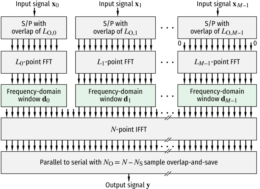
Figure 2: Original FC-based synthesis filter bank structure. In this structure, only the FD windows are adjustable.

II-A Original Fast-Convolution Filter-Bank Schemes

The application of FC to multirate filters has been presented in [19], and FC realizations of channelization filters have been considered in [20, 21, 22]. The analysis and optimization methods for FC-implementation of nearly perfect-reconstruction filter-bank systems are developed in [23]. Original FC-based synthesis filter-bank structure proposed in [23] is depicted in Fig. 2, for a case where $M$ incoming low-rate, narrowband signals $\mathbf{x}_{m}$ for $m=0,1,\dots,M-1$ with adjustable frequency responses and adjustable sampling rates are to be combined into single wideband signal $\mathbf{y}$. This structure efficiently combines the multirate FC-based filtering and the straightforward representations of the desired frequency-responses with the OLS processing to provide, e.g., a generic waveform processing engine for evolving cellular mobile communications systems. The dual structure can be used on the RX side as an analysis filter bank (AFB) for splitting the incoming high-rate, wideband signal into several narrowband signals [24]. Consequently, FC approach has been applied for filter-bank multicarrier waveforms in [25] and for flexible single-carrier (SC) waveforms in [26]. An optimization-based framework for FC-F-OFDM waveform processing for 5G-NR physical layer is developed and evaluated in [13].

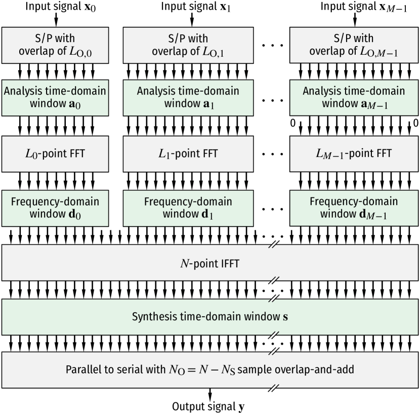
Figure 3: Proposed generalized FC-based flexible synthesis filter bank structure. In this structure, the analysis and synthesis TD windows as well as the FD windows are adjustable.

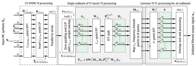
Figure 4: Proposed generalized FC-F-OFDM transmitter. The processing structure for subband $m$ is shown (cf. Fig. 3 for the overall synthesis processing). The long $N$-point IFFT is common for all the subbands. The OFDM TX processing shown by the dashed block is the same for both the original and generalized schemes. The CP-OFDM TX processing is described by (3) and (4) while the TX FC processing is described by (12) and (15) (or alternatively by (16)).

II-B Proposed Generalized Fast-Convolution-based Filtered OFDM

In this article, we describe a generalized FC processing model providing an improved performance with specific application to subband-filtered CP-OFDM TX processing. The generalized FC processing is optimized and analyzed based on the assumption of a plain CP-OFDM RX, following the basic principles of transparent signal processing [6]. Fig. 3 shows the proposed generalized FC synthesis filter-bank structure. In this structure, each of the $M$ signals to be transmitted is first segmented into overlapping processing blocks of length $L_{m}$ with overlap of $L_{\text{O},m}$ samples. Let us denote the non-overlapping part by $L_{\text{S},m}=L_{m}-L_{\text{O},m}$ and the overlap factor by $\lambda=1-L_{\text{S},m}/L_{m}$. Then, each input block is multiplied element-wise by TD analysis window $\mathbf{a}_{m}$ and transformed to frequency domain using $L_{m}$-point FFT. The FD bin values of each converted subband signal are multiplied by the FD window $\mathbf{d}_{m}$ corresponding to the FFT of the finite-length linear filter impulse response. Finally, the weighted signals are combined and converted back to time domain using $N$-point IFFT and the resulting TD output blocks are multiplied by the synthesis window $\mathbf{s}$ and concatenated using the OLA principle such that the overlap between consecutive blocks is $N_{\text{O}}=\lambda N$ samples.

In FC-based subband-filtered OFDM (FC-F-OFDM), FC-based filtering is applied at subband level, corresponding to one or multiple contiguous PRBs with same SCS, while utilizing normal CP-OFDM waveform for the PRBs [15, 16, 13]. With FC-F-OFDM processing, it is very straightforward to adjust the bandwidths of the subbands individually. This is useful in subband-filtered OFDM since there is no need to realize guard bands and filter transition bands between synchronous subbands with the same numerology. In the extreme case, as will be considered in Section V, the group of filtered PRBs could cover the full carrier bandwidth, and thus the tight channelization filtering for the whole carrier is realized by the FC processing.

Fig. 4 illustrates the proposed generalized FC-F-OFDM TX processing for $m$th subband. The TD OFDM signal $\mathbf{X}_{\text{OFDM},m}$ is obtained from FD symbols $\mathbf{X}_{m}$ with $L_{\text{ACT},m}$ active subcarriers by taking the $L_{\text{OFDM},m}$-point IFFT, that is, with zero-padding of $L_{\text{OFDM},m}-L_{\text{ACT},m}$ subcarriers. Then, CP of length $L_{\text{CP},m}$ is inserted and the resulting CP-OFDM signal $\mathbf{X}_{\text{CP-OFDM},m}$ is converted from parallel to serial for FC processing.

Formally, CP-OFDM TX processing of the $m$th subband can be expressed as

$$\mathbf{X}_{\text{CP-OFDM},m}=\mathbf{K}_{L_{\text{CP},m}}\widehat{\mathbf{W}}_{L_{\text{OFDM},m}}^{-1}\mathbf{X}_{m},$$ (3a)

where $$\mathbf{X}_{m}\in\mathbb{C}^{L_{\text{OFDM},m}\times B_{\text{OFDM},m}} \mathcal{M} \mathcal{M} \widehat{\mathbf{W}}^{-1}_{L_{\text{OFDM},m}}\in\mathbb{C}^{L_{\text{OFDM},m}\times L_{\text{OFDM},m}} \sqrt{L_{\text{OFDM},m}} \mathbf{K}_{L_{\text{CP},m}}\in\mathbb{N}^{(L_{\text{OFDM},m}+L_{\text{CP},m})\times L_{\text{OFDM},m}}$$ is the matrix containing the incoming quadrature phase-shift keying (QPSK) or -ary quadrature amplitude modulation (-QAM) symbols (with power normalized to unity), is the inverse discrete Fourier transform (IDFT) matrix scaled by a factor of , and is the CP insertion matrix as given by

$$\mathbf{K}_{L_{\text{CP},m}}=\begin{bmatrix}\begin{matrix}\mathbf{0}_{L_{\text{CP},m}\times(L_{\text{OFDM},m}-L_{\text{CP},m})}&\mathbf{I}_{L_{\text{CP},m}}\end{matrix}\\[2.0pt] \mathbf{I}_{L_{\text{OFDM},m}}\end{bmatrix}.$$ (3b)

Here, $\mathbf{I}_{q}$ is $q\times q$ identity matrix and $\mathbf{0}_{q\times p}$ is $q\times p$ zero matrix.

Alternatively, CP-OFDM TX processing can be represented as

$$\mathbf{x}_{\text{CP-OFDM},m}=\mathbf{T}_{\text{BD,TX},m}\mathbf{x}_{m},$$ (4a)

where $$\mathbf{T}_{\text{BD,TX},m}\in\mathbb{C}^{(L_{\text{OFDM},m}+L_{\text{CP},m})B_{\text{OFDM},m}\times L_{\text{OFDM},m}B_{\text{OFDM},m}}$$ is block-diagonal CP-OFDM modulation matrix given by

$$\mathbf{T}_{\text{BD,TX},m}=\operatorname{diag}\Big{(}\underbrace{\mathbf{T}_{\text{TX},m},\mathbf{T}_{\text{TX},m},\dots,\mathbf{T}_{\text{TX},m}}_{\text{$B_{\text{OFDM},m}$ blocks}}\Big{)}$$ (4b)

with non-overlapping blocks $$\mathbf{T}_{\text{TX},m}=\mathbf{K}_{L_{\text{CP},m}}\widehat{\mathbf{W}}_{L_{\text{OFDM},m}}^{-1} \mathbf{x}_{m}=\operatorname{vec}(\mathbf{X}_{m}) m$$ and is the column vector formed by stacking vertically the input symbols on subband as follows:

$$\mathbf{x}_{m}=\begin{bmatrix}[\mathbf{X}_{m}]^{\mathchoice{\raisebox{0.0pt}{$\displaystyle\intercal$}}{\raisebox{0.0pt}{$\textstyle\intercal$}}{\raisebox{0.0pt}{$\scriptstyle\intercal$}}{\raisebox{0.0pt}{$\scriptscriptstyle\intercal$}}}_{1}&[\mathbf{X}_{m}]^{\mathchoice{\raisebox{0.0pt}{$\displaystyle\intercal$}}{\raisebox{0.0pt}{$\textstyle\intercal$}}{\raisebox{0.0pt}{$\scriptstyle\intercal$}}{\raisebox{0.0pt}{$\scriptscriptstyle\intercal$}}}_{2}&\cdots&[\mathbf{X}_{m}]^{\mathchoice{\raisebox{0.0pt}{$\displaystyle\intercal$}}{\raisebox{0.0pt}{$\textstyle\intercal$}}{\raisebox{0.0pt}{$\scriptstyle\intercal$}}{\raisebox{0.0pt}{$\scriptscriptstyle\intercal$}}}_{B_{\text{OFDM},m}}\end{bmatrix}^{\mathchoice{\raisebox{0.0pt}{$\displaystyle\intercal$}}{\raisebox{0.0pt}{$\textstyle\intercal$}}{\raisebox{0.0pt}{$\scriptstyle\intercal$}}{\raisebox{0.0pt}{$\scriptscriptstyle\intercal$}}}.$$ (4c)

Here, $[\mathbf{X}_{m}]_{k}$ denotes the $k$th column of matrix $\mathbf{X}_{m}$. In the structure of Fig. 4, the OFDM TX processing module generates samples for the overall symbol duration of $L_{\text{OFDM},m}+L_{\text{CP},m}$ for $B_{\text{OFDM},m}$ symbols. The FC-filtering process increases the sampling rate by the factor of

$$I_{m}=N/L_{m},$$ (5)

resulting in OFDM symbol and CP durations of $N_{\text{OFDM},m}=I_{m}L_{\text{OFDM},m}$ and $N_{\text{CP},m}=I_{m}L_{\text{CP},m}$, respectively. Here $L_{\text{OFDM},m}$ and $L_{\text{CP},m}$ have integer values. It is convenient, but not necessary, that $N_{\text{OFDM},m}$ and $N_{\text{CP},m}$ have integer values as well.

II-C Proposed Generalized Model for FC Synthesis Filter Bank

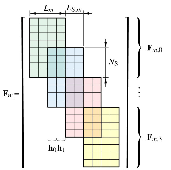
Figure 5: Structure of block-diagonal synthesis matrix $\mathbf{F}_{m}$ for four ($R_{m}=4$) FC processing blocks with $L_{m}=4$, $N=8$, and $N_{\text{S}}=2L_{\text{S},m}=4$ ($\lambda=1/2$). The colored $8\times 4$ rectangles illustrate the overlapping processing blocks $\mathbf{F}_{m,r}$ for $r=0,1,2,3$. The impulse responses of the processing are given by the columns $[\mathbf{F}_{m}]_{k}$ for $k=3,4,\dots,8$ of the $\mathbf{F}_{m}$. Here, $h_{0}$ is given by the columns $[\mathbf{F}_{m}]_{k}$ for $k=3,5,7$ and $h_{1}$ by the columns $[\mathbf{F}_{m}]_{k}$ for $k=4,6,8$.

In the generalized FC synthesis filter bank (SFB) case, the block processing of $m$th CP-OFDM subband signal $\mathbf{x}_{\text{CP-OFDM},m}$ of length

$$T_{m}=B_{\text{OFDM},m}(L_{\text{OFDM},m}+L_{\text{CP},m})$$ (6)

for the generation of high-rate subband waveform $\mathbf{w}_{m}$ can be represented as

$$\mathbf{w}_{m}=\mathbf{F}_{m}\textbf{x}_{\text{ZP},m},$$ (7a)

where $$\mathbf{F}_{m}$$ is the block diagonal transform matrix of the form

$$\mathbf{F}_{m} =\operatorname{bdiag}\left(\mathbf{F}_{m,0},\mathbf{F}_{m,1},\dots,\mathbf{F}_{m,R_{m}-1}\right)_{L_{\text{O},m},N_{\text{O}}}$$ (7b)

with overlapping blocks $$\mathbf{F}_{m,r}\in\mathbb{C}^{N\times L_{m}} r=0,1,\dots,R_{m}-1$$ for , as illustrated in Fig. 5, and

$$\mathbf{x}_{\text{ZP},m}=\begin{bmatrix}\mathbf{0}_{1\times S_{\text{F},m}}&\mathbf{x}_{\text{CP-OFDM},m}^{\mathchoice{\raisebox{0.0pt}{$\displaystyle\intercal$}}{\raisebox{0.0pt}{$\textstyle\intercal$}}{\raisebox{0.0pt}{$\scriptstyle\intercal$}}{\raisebox{0.0pt}{$\scriptscriptstyle\intercal$}}}&\mathbf{0}_{1\times S_{\text{F},m}}\end{bmatrix}^{\mathchoice{\raisebox{0.0pt}{$\displaystyle\intercal$}}{\raisebox{0.0pt}{$\textstyle\intercal$}}{\raisebox{0.0pt}{$\scriptstyle\intercal$}}{\raisebox{0.0pt}{$\scriptscriptstyle\intercal$}}}.$$ (7c)

The input signal $\mathbf{x}_{\text{CP-OFDM},m}$ has to be padded in the beginning and end by at least

$$S_{\text{F},m}=L_{m}-L_{\text{S},m}$$ (8)

zero-valued samples in order to carry out the processing such that all the incoming samples are facing the same impulse responses (cf. Fig. 5). Now, the first sample after the zero-padding is convolved by the impulse response given by $S_{\text{F},m}+1$th column of $\mathbf{F}_{m}$, that is, by $\mathbf{h}_{0}=[\mathbf{F}_{m}]_{S_{\text{F},m}+1}$ whereas the second sample is convolved by $\mathbf{h}_{1}=[\mathbf{F}_{m}]_{S_{\text{F},m}+2}$. Assuming that all the $\mathbf{F}_{m,r}$’s are the same, then the processing determined by (7) is periodically shift variant in the sense that there are altogether $L_{\text{S},m}$ impulse responses such that every $L_{\text{S},m}$th sample experiences the same impulse response.

The number of FC-processing blocks is given by,

$$R_{m}=\left\lceil\left(2S_{\text{F},m}+T_{m}-L_{m}\right)/L_{\text{S},m}\right\rceil+1.$$ (9)

The number of blocks can be different for different subbands provided that processing is carried for

$$R_{\text{max}}=\max_{m=0,1,\dots,M-1}(R_{m})$$ (10)

blocks. The overall waveform to be transmitted is obtained by summing all the $M$ subband waveforms as

$$\mathbf{z_{\text{FC-F-OFDM}}}=\sum_{m=0}^{M-1}\mathbf{w}_{m}.$$ (11)

The generalized FC SFB shown in Fig. 4 can be represented using block processing by decomposing the $\mathbf{F}_{m,r}$’s as follows:

$$\mathbf{F}_{m,r}=\sqrt{N/L_{m}}\mathbf{S}\mathbf{U}_{m}\mathbf{C}_{m}\mathbf{A}_{m},$$ (12a)

where $$\mathbf{A}_{m}\in\mathbb{R}^{L_{m}\times L_{m}} \mathbf{S}\in\mathbb{R}^{N\times N} \mathbf{a}_{m} \mathbf{s}$$ and are the TD analysis and synthesis windowing matrices with the analysis and synthesis window weights and , respectively, on their diagonals and

$$\mathbf{C}_{m}=\mathbf{W}^{-1}_{L_{m}}\mathbf{D}_{m}\mathbf{P}^{(\lceil L_{m}/2\rceil)}_{L_{m}}\mathbf{W}_{L_{m}}$$ (12b)

corresponds to the circular-convolution matrix with discrete Fourier transform (DFT) shifted processing blocks while

$$\mathbf{U}_{m}=\mathbf{W}^{-1}_{N}\mathbf{M}_{m,r}\mathbf{W}_{L_{m}}$$ (12c)

is the interpolation matrix corresponding to zero padding and circular shifting in frequency domain. The first term in (12b) and the last term in (12c) cancel out in (12a), however, those terms are shown here for emphasizing the processing carried out by (12b) and (12c). Here, $\mathbf{W}_{L_{m}}\in\mathbb{C}^{L_{m}\times L_{m}}$ and $\mathbf{W}_{N}^{-1}\in\mathbb{C}^{N\times N}$ are the $L_{m}\times L_{m}$ DFT matrix and $N\times N$ inverse DFT matrix, respectively. $\mathbf{P}^{(\lceil L_{m}/2\rceil)}_{m}\in\mathbb{Z}^{L_{m}\times L_{m}}$ is the DFT shift matrix obtained by cyclically shifting the $L_{m}\times L_{m}$ identity matrix right by $\lceil L_{m}/2\rceil$ positions while the FD mapping matrix $\mathbf{M}_{m,r}\in\mathbb{C}^{N\times L_{m}}$ maps $L_{m}$ FD bins of the input signal to FD bins $(c_{m}-\lceil L_{m}/2\rceil+\ell\bmod N)$ for $\ell=0,1,\dots,L_{m}-1$ of the output signal. Here $c_{m}$ is the center bin of the subband $m$. In addition, this matrix rotates the phase of the processing block by

$$\Theta_{m}(r)=\exp({\mathop{\mspace{1.0mu}\mathrm{j}\mspace{0.5mu}}\nolimits}2\pi{r}\theta_{m})\quad\text{with}\quad\theta_{m}=c_{m}L_{\text{S},m}/L_{m}$$ (13)

in order to maintain the phase continuity between the consecutive overlapping blocks [23]. The FD windowing matrix $\mathbf{D}_{m}\in\mathbb{R}^{L_{m}\times L_{m}}$ is a diagonal matrix with the FD window weights $\mathbf{d}_{m}$ of the subband $m$ on its main diagonal, expressed as

$$\mathbf{D}_{m}=\operatorname{diag}(\mathbf{d}_{m}).$$ (14)

The time-domain equivalent of the proposed processing is given by (12a). As seen from this equation, the analysis windows are applied for each subband separately so this provides a way to adjust the frequency-domain localization of each subband. The filtering realized through FC processing in $\mathbf{C}_{m}$ provides computationally efficient realization for the convolution with high flexibility in adjusting the bandwidth of the subband. Considering the interpolation process described by $\mathbf{U}_{m}$, it enables to easily combine and modulate the subband signals to their desired locations with the granularity of FC processing bin spacing. However, by inspecting (12c) it can be noticed that interpolation provided by interpolating FC processing corresponds to the frequency-domain zero-padding a.k.a. sinc-interpolation. This equation does not provide any way to control the frequency-response of the interpolator since $\mathbf{M}_{m,r}$ maps $L_{m}$ frequency-domain bins of the subband signal to $N$ bins of the output signal and these $L_{m}$ bins are already weighted by the frequency-domain window in $\mathbf{C}_{m}$. On the other hand, the time-domain synthesis window provides additional control for the time-domain localization over the interpolated composite waveform and thus contributes to the spectral localization to certain extent.

The matrix model determined by (7) and (12) can be used for analysis and optimization purposes whereas for efficient implementation with real-time hardware or software, it is beneficial to divide the input data into overlapping blocks and carry out the processing for $r=0,1,\dots,R_{\text{max}}-1$ as

$$\mathbf{w}_{\text{BUFF},m,r}=\textbf{F}_{m,r}\mathbf{x}_{\text{BUFF},m,r}.$$ (15a)

Here, $$\mathbf{x}_{\text{BUFF},m,r} r \mathbf{x}_{\text{ZP},m}$$ is the th processing block of as expressed by

$$[\mathbf{x}_{\text{BUFF},m,r}]_{k}=[\mathbf{x}_{\text{ZP},m}]_{rL_{\text{S},m}+k}$$ (15b)

for $$k=1,2,\dots,L_{m}$$. The high-rate subband waveform can be obtained by overlap-and-add processing as given by

$$\mathbf{w}_{m}=\sum_{r=0}^{R_{\text{max}}-1}\boldsymbol{\Gamma}_{r}\mathbf{w}_{\text{BUFF},m,r},$$ (15c)

where

$$\boldsymbol{\Gamma}_{r}=\begin{bmatrix}\mathbf{0}_{N\times rN_{\text{S}}}&\mathbf{I}_{N}&\mathbf{0}_{N\times(R_{\text{max}}-1)N_{\text{S}}-rN_{\text{S}}}\end{bmatrix}^{\mathchoice{\raisebox{0.0pt}{$\displaystyle\intercal$}}{\raisebox{0.0pt}{$\textstyle\intercal$}}{\raisebox{0.0pt}{$\scriptstyle\intercal$}}{\raisebox{0.0pt}{$\scriptscriptstyle\intercal$}}}$$ (15d)

overlaps the processed blocks to their desired time-domain locations. The buffering, as expressed by (15a), and overlap-and-add processing, as expressed by (15d), are denoted in Fig. 4 by $\operatorname{buff}(\cdot)$ and $\operatorname{ola}(\cdot)$, respectively.

By following the above formulation, the overall FC TX processing can be compactly expressed in three steps: (i) Buffering of the OFDM modulated and zero-padded waveforms for $m=0,1,\dots,M-1$ into the overlapping blocks for $r=0,1,\dots,R_{\text{max}}-1$ and for $k=1,2,\dots,L_{m}$ as given by

$$[\mathbf{x}_{\text{BUFF},m,r}]_{k}=\begin{bmatrix}\mathbf{0}_{S_{\text{F},m}\times 1}\\ \operatorname{vec}\left(\mathbf{K}_{L_{\text{CP},m}}\widehat{\mathbf{W}}_{L_{\text{OFDM},m}}\mathbf{X}_{m}\right)\\ \mathbf{0}_{S_{\text{F},m}\times 1}\end{bmatrix}_{rL_{\text{S},m}+k}.$$ (16a)

(ii) Processing of the blocks and combining the subbands in frequency domain, expressed as

$$\mathbf{v}_{\text{BUFF},r}=\sum_{m=0}^{M-1}\sqrt{\frac{N}{L_{m}}}\mathbf{M}_{m,r}\mathbf{D}_{m}\mathbf{P}^{(\lceil L_{m}/2\rceil)}_{L_{m}}\mathbf{W}_{L_{m}}\mathbf{A}_{m}\mathbf{x}_{\text{BUFF},m,r}.$$ (16b)

(iii) Converting the overall waveform to time-domain and concatenating the processed blocks as given by

$$\mathbf{z}_{\text{FC-F-OFDM}}=\sum_{r=0}^{R_{\text{max}}-1}\boldsymbol{\Gamma}_{r}\mathbf{S}\mathbf{W}^{-1}_{N}\mathbf{V}_{\text{BUFF},r},$$ (16c)

where $\boldsymbol{\Gamma}_{r}$ is given by (15d).

Due to the overlapping block processing in FC-based filter bank, one CP-OFDM symbol is divided into multiple FC processing blocks and, in general, these processing blocks are not time aligned with the CP-OFDM symbols in the case of non-zero and possibly varying CP lengths. Fig. 6 depicts an example of block processing for one CP-OFDM symbol in the case when the ratio of $N$ and $L_{m}$ is two and the overlap is $50\text{\,}\%$ ($\lambda=1/2$). For continuous processing of multiple symbols the overhead due to zero-padding and the unmatched FC processing block and CP-OFDM symbol lengths diminishes as the number of symbols increases and at minimum only one additional FC-processing block is needed for overlap of $50\text{\,}\%$.

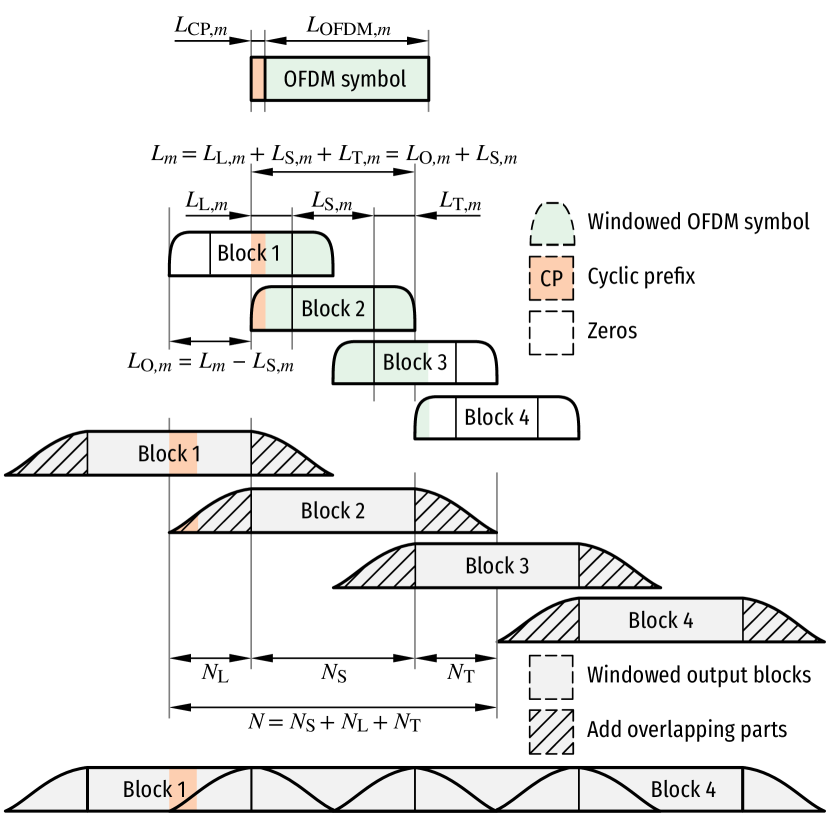
Figure 6: Example case where four overlapping blocks are required for processing one CP-OFDM symbol with $50\text{\,}\%$ overlap.

In the multirate version of the conventional OLS scheme, the incoming signals are first segmented into overlapping data segments of length $L_{m}$ and then from the processed output segments, $N_{\text{O}}=N-N_{\text{S}}$ samples are discarded in order to match the number of input and output samples. Using the above generalized model given by (12), this scheme can be achieved by determining the TD analysis and synthesis windowing matrices as

$$\mathbf{A}_{m}=\mathbf{I}_{L_{m}}\quad\text{and}\quad\mathbf{S}=\operatorname{diag}\left(\begin{bmatrix}\mathbf{0}_{1\times N_{\text{L}}}&\mathbf{1}_{1\times N_{\text{S}}}&\mathbf{0}_{1\times N_{\text{T}}}\end{bmatrix}^{\mathchoice{\raisebox{0.0pt}{$\displaystyle\intercal$}}{\raisebox{0.0pt}{$\textstyle\intercal$}}{\raisebox{0.0pt}{$\scriptstyle\intercal$}}{\raisebox{0.0pt}{$\scriptscriptstyle\intercal$}}}\right),$$ (17)

respectively. Here, the number of overlapping samples $N_{\text{O}}=N-N_{\text{S}}$ is divided into leading and tailing overlapping parts as follows:

$$N_{\text{L}}=\left\lceil\frac{N-N_{\text{S}}}{2}\right\rceil\quad\text{and}\quad N_{\text{T}}=\left\lfloor\frac{N-N_{\text{S}}}{2}\right\rfloor.$$ (18)

The corresponding leading and tailing overlapping parts of the $L_{m}$ are denoted by $L_{\text{L},m}$ and $L_{\text{T},m}$, respectively.

In the case of multirate version of the conventional OLA scheme, the non-overlapping input data blocks are zero-padded to length $L_{m}$ and the output blocks are overlapped and added such that the number of input and output samples match as desired. For the proposed generalized model, this is achieved by selecting the analysis and synthesis windowing matrices as

$$\mathbf{A}_{m}=\operatorname{diag}\left(\begin{bmatrix}\mathbf{0}_{L_{1\times\text{L},m}}&\mathbf{1}_{L_{1\times\text{S},m}}&\mathbf{0}_{L_{1\times\text{T},m}}\end{bmatrix}^{\mathchoice{\raisebox{0.0pt}{$\displaystyle\intercal$}}{\raisebox{0.0pt}{$\textstyle\intercal$}}{\raisebox{0.0pt}{$\scriptstyle\intercal$}}{\raisebox{0.0pt}{$\scriptscriptstyle\intercal$}}}\right)\quad\text{and}\quad\mathbf{S}=\mathbf{I}_{N},$$ (19)

respectively.

For the proposed generalized model, in addition to the FD window, also the analysis and synthesis TD windows are adjustable and the FC-based filter-bank design is carried out by optimizing all the windows simultaneously. The main target of the TD analysis window is to improve the spectral localization of the incoming CP-OFDM waveform by properly weighting the samples interpolated by the frequency-domain zero-padding in OFDM modulation. This windowing may induce some additional replicas in the spectrum which are filtered by the following FD windowing. The target of the synthesis window is to smoothen the discontinuities between the overlapping blocks as well as the beginning and end transients since the discontinuities in the output waveform give raise to a high spectral leakage. For latency-critical applications, the zero-padding (cf. (7c)) in the beginning of the burst can also be reduced and especially in this case, the synthesis windowing of the filtered blocks becomes crucial.

When the FC-based filter bank is used for processing the OFDM signals, the OFDM symbol subcarrier spacing on subband $m$ is determined as

$$f_{\text{SCS},m}=\frac{f_{\text{s},m}}{L_{\text{OFDM},m}}=\frac{L_{m}}{N}\frac{f_{\text{s}}}{L_{\text{OFDM},m}},$$ (20)

where, $f_{\text{s}}$ is the output sampling rate and $f_{\text{s},m}$ is the input sampling rate for subband $m$, which can be selected independently for each subband. The above equation defines $L_{m}$, given the subcarrier spacing for subband $m$, output sampling rate $f_{\text{s}}$, and FC IFFT length $N$. It should also be pointed out that the bin spacing (BS) in FC processing as given by

$$f_{\text{BS},m}=\frac{f_{\text{s}}}{N},$$ (21)

can be selected to be greater than, smaller than, or equal to subcarrier spacing in OFDM processing by properly choosing $N$ and $L_{m}$. For more details for the parameterization of the original FC processing schemes, see [23, 15, 13]. In practice, $f_{\text{BS},m}$ is typically fixed, and the supported OFDM subcarrier spacings and sampling rates define the used FC FFT lengths $L_{m}$.

II-D OFDM RX Processing

In the case, when FC interpolation factor $I_{m}=N/L_{m}>1$, the FC-F-OFDM waveform can be received transparently with basic CP-OFDM receiver by either using the OFDM demodulator running at the high input rate or by first decimating the high-rate signal by $N/L_{m}$ and then using the demodulator on the decimated rate. In the former case, the basic CP-OFDM RX processing of the $m$th subband on the receiver side can be expressed as

$$\mathbf{Y}_{m}=\widehat{\mathbf{W}}_{N_{\text{OFDM},m}}\mathbf{R}_{N_{\text{CP},m}}\tilde{\mathbf{Z}}_{\text{FC-F-OFDM}},$$ (22a)

where $$\widehat{\mathbf{W}}_{N_{\text{OFDM},m}}\in\mathbb{C}^{N_{\text{OFDM},m}\times N_{\text{OFDM},m}} 1/\sqrt{N_{\text{OFDM},m}} \mathbf{R}_{N_{\text{CP},m}}\in\mathbb{Z}^{N_{\text{OFDM},m}\times(N_{\text{OFDM},m}+N_{\text{CP},m})}$$ is the DFT matrix scaled by and is the CP removal matrix given by

$$\mathbf{R}_{N_{\text{CP},m}}=\left[\begin{matrix}\mathbf{0}_{N_{\text{OFDM},m}\times N_{\text{CP},m}}&\mathbf{I}_{N_{\text{OFDM},m}}\end{matrix}\right].$$ (22b)

The received signal is modelled by

$$\tilde{\mathbf{Z}}_{\text{FC-F-OFDM}}=\operatorname{vec}^{-1}(\tilde{\mathbf{z}}_{\text{FC-F-OFDM}}),$$ (22c)

which is an $$(N_{\text{OFDM},m}+N_{\text{CP},m})\times B_{\text{OFDM},m} (N_{\text{OFDM},m}+N_{\text{CP},m})B_{\text{OFDM},m} \tilde{\mathbf{z}}_{\text{FC-F-OFDM}}$$ matrix formed by un-stacking the samples from the received sequence . For TX performance analysis and optimization purposes, the received sequence is defined as

$$\tilde{\mathbf{z}}_{\text{FC-F-OFDM}}=\mathbf{R}_{\text{ZP},m}\mathbf{z}_{\text{FC-F-OFDM}}.$$ (22d)

where

$$\mathbf{R}_{\text{ZP},m}=\begin{bmatrix}\mathbf{0}_{N/L_{m}S_{\text{F},m}\times N/L_{m}T_{m}}\\ \mathbf{I}_{N/L_{m}T_{m}}\\ \mathbf{0}_{N/L_{m}S_{\text{F},m}\times N/L_{m}T_{m}}\end{bmatrix}^{\mathchoice{\raisebox{0.0pt}{$\displaystyle\intercal$}}{\raisebox{0.0pt}{$\textstyle\intercal$}}{\raisebox{0.0pt}{$\scriptstyle\intercal$}}{\raisebox{0.0pt}{$\scriptscriptstyle\intercal$}}}$$ (22e)

discards the zero padding (cf. (7c)) by removing first and last $$N/L_{m}S_{\text{F},m}$$ samples from the high-rate signal before further RX processing.

In the latter case, when the signal after the discarding of zero padding is decimated by $N/L_{m}$ before the OFDM demodulation, the OFDM RX processing is expressed as

$$\mathbf{Y}_{m}=\widehat{\mathbf{W}}_{L_{\text{OFDM},m}}\mathbf{R}_{L_{\text{CP},m}}\bar{\mathbf{Z}}_{\text{FC-F-OFDM}},$$ (23a)

where $$\bar{\mathbf{Z}}_{\text{FC-F-OFDM}} (L_{\text{OFDM},m}+L_{\text{CP},m})\times B_{\text{OFDM},m} L_{\text{OFDM},m}\times L_{\text{OFDM},m}$$ is an matrix containing the received samples, the scaled DFT matrix is of size , and the CP removal matrix is given by

$$\mathbf{R}_{L_{\text{CP},m}}=\left[\begin{matrix}\mathbf{0}_{L_{\text{OFDM},m}\times L_{\text{CP},m}}&\mathbf{I}_{L_{\text{OFDM},m}}\end{matrix}\right].$$ (23b)

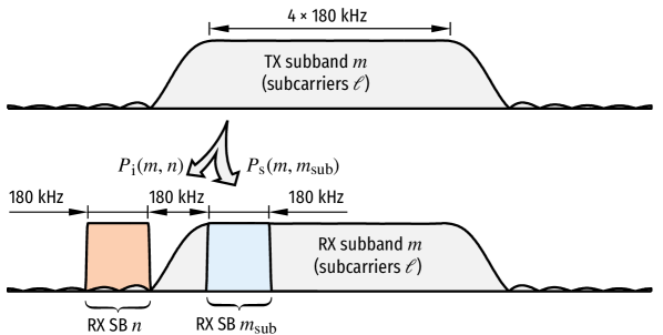
Figure 7: Illustration of the spectral confinement ratio (SCR) evaluation. The level of observable power $P_{\text{s}}(m,m_{\text{sub}})$ and leaking power $P_{\text{i}}(m,n)$ are measured over the fixed bandwidth of $180\text{\,}\mathrm{k}\mathrm{H}\mathrm{z}$ which corresponds to a single PRB when SCS is $15\text{\,}\mathrm{k}\mathrm{H}\mathrm{z}$.

III Fast-Convolution Filter-Bank Optimization

In this article, as formulated in Section II, we are using the generalized FC processing for improving the spectral containment of CP-OFDM waveform on the TX side. The exact RX processing is generally not known due to the transparent signal processing assumption [5, 6] and, therefore, when it comes to quantifying the band-limitation of the TX signal subbands, we are measuring the TX power leakage by using narrow-band TD measurement filter with bandwidth equal to one PRB. By using this approach, the TX processing frequency selectivity can be accurately measured independent of the exact RX processing and subcarrier spacings by locating the unintended RX on subband $n$ in the close vicinity of target subband $m$ as illustrated in Fig. 7. The observable power on target subband $m$ is measured using the same narrow-band filter such that the filter is located at the edge of the subband. The optimization target is then to constrain the in-band unwanted emissions (inside one carrier) and in particular the interference leakage between different subbands, with possibly different numerologies or asynchronous transmissions, without considerably increasing the intrinsic passband distortion induced by the FC-based subband filtering process.

III-A Performance Metrics

We define the so-called spectral confinement ratio (SCR) as the metric for characterizing unwanted in-band (inside one carrier) or out-of-band emissions. The power on subband $m$ and $n$ is measured using fixed bandwidth of $180\text{\,}\mathrm{k}\mathrm{H}\mathrm{z}$ (one PRB with $15\text{\,}\mathrm{k}\mathrm{H}\mathrm{z}$ baseline SCS) with the aid of a narrow-band finite impulse response (FIR) measurement filter. The observable power $P_{\text{s}}{(m,m_{\text{sub}})}$ is obtained by locating the measurement filter over the edge subcarriers while the leaking power $P_{\text{i}}{(m,n)}$ is measured over the band starting $180\text{\,}\mathrm{k}\mathrm{H}\mathrm{z}$ from the subband edge. The $180\text{\,}\mathrm{k}\mathrm{H}\mathrm{z}$ guard band is selected because it corresponds to the resolution by which bandwidth parts can be allocated in the 5G-NR [1, Section 7.3], for carrier frequencies below $6\text{\,}\mathrm{G}\mathrm{H}\mathrm{z}$ [27, Section 4.4.4.2]. Now, SCR is formally defined as

$$\mathrm{SCR}_{m}=10\log_{10}\left(\frac{P_{\text{i}}{(m,n)}}{P_{\text{s}}{(m,m_{\text{sub}})}}\right),$$ (24)

where $P_{\text{i}}{(m,n)}$ is the power leaking from subband $m$ to subband $n$ and $P_{\text{s}}{(m,m_{\text{sub}})}$ is the observable power on the subset of subband $m$. In the actual numerical examples and evaluations reported in Section V, the transition bandwidth of the measurement filter is $7.5\text{\,}\mathrm{k}\mathrm{H}\mathrm{z}$ (half of the $15\text{\,}\mathrm{k}\mathrm{H}\mathrm{z}$ baseline SCS) and the minimum stopband attenuation is $A_{\text{s}}=$100\text{\,}\mathrm{d}\mathrm{B}$$. The corresponding magnitude response of the measurement TD filter is show in Fig. 8.

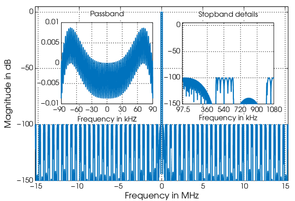
Figure 8: Magnitude response as well as the passband and stopband details of the measurement FIR filter for evaluating the spectral confinement ratio (SCR). Here, passband is one PRB ($180\text{\,}\mathrm{k}\mathrm{H}\mathrm{z}$) wide and the transition band is one-half ($7.5\text{\,}\mathrm{k}\mathrm{H}\mathrm{z}$) of a baseline subcarrier spacing of $15\text{\,}\mathrm{k}\mathrm{H}\mathrm{z}$.

The passband quality on an active subcarrier $\ell$ and on subband $m$ is measured using the mean-squared error (MSE) between the (normalized) transmitted and received symbols as follows:

$$\text{MSE}_{m}(\ell)=\lvert\lvert[\mathbf{X}_{m}]_{\ell,s}-[\mathbf{Y}_{m}]_{\ell,s}\rvert\rvert^{2},$$ (25)

where $[\mathbf{X}_{m}]_{\ell,s}$ and $[\mathbf{Y}_{m}]_{\ell,s}$, respectively, are the transmitted and received symbols on subcarrier $\ell$ and $s\in\{1,2,\ldots,B_{\text{OFDM},m}\}$. The corresponding error vector magnitude (EVM) in percents is expressed using (25) as

$$\text{EVM}_{m}(\ell)=100\sqrt{\text{MSE}_{m}(\ell)}.$$ (26)

The MSE and EVM are measured after executing zero-forcing (ZF) equalization, as defined in 3GPP 5G-NR specification in [28, Annex B].

The average MSE is defined as the mean value of the MSE values on active subcarriers, as given by

$$\text{MSE}_{\text{AVG},m}=\frac{1}{{L}_{\text{ACT},m}}\sum_{\ell=0}^{{L}_{\text{ACT},m}-1}\text{MSE}_{m}(\ell).$$ (27)

For the analysis purposes we also quantify the worst-case MSE. This is determined as a mean value of the MSE over the edge subcarriers as given by

$$\text{MSE}_{\text{MAX},m}=\frac{1}{\lvert\mathcal{E}_{\text{L}}\cup\mathcal{E}_{\text{R}}\rvert}\sum_{\begin{subarray}{c}\ell=\mathcal{E}_{\text{L}}\cup\mathcal{E}_{\text{R}}\end{subarray}}\text{MSE}_{m}(\ell).$$ (28)

Here, $\mathcal{E}_{\text{L}}=\{0,1,\dots,N_{\text{edge}}-1\}$ and $\mathcal{E}_{\text{R}}=\{{L}_{\text{ACT},m}-N_{\text{edge}},{L}_{\text{ACT},m}-N_{\text{edge}}+1,\dots,{L}_{\text{ACT},m}-1\}$ denote the left and right edge subcarriers, respectively. The number of edge subcarriers is selected to be $N_{\text{edge}}=12$. This metric is also in-line with the edge PRB EVM measurement defined and presented in [29].

III-B Parameterization of Time- and Frequency-domain Windows

For simplicity, we consider the optimization of windows with even lengths. For the proposed model, in general, all the weights of the windows are adjustable. However, in the case of FD window, it has turned out that it is beneficial to select the window such that the weights on subband $m$ consist of two symmetric transition bands with non-trivial values $\xi_{m}(p)$ for $p=0,1,\dots,L_{\text{TBW},m}-1$, where $L_{\text{TBW},m}$ also defines the transition-band width. All passband weights are set to one and all stopband weights are set to zero. The number of stopband weights (and the corresponding transform length $L_{m}$) can be selected to reach a feasible subband oversampling factor. Now the diagonal weight values in (14) can be expressed as

$$\mathbf{d}_{m} =\bigl{[}\begin{matrix}\mathbf{0}_{1\times(\lceil[L_{m}-L_{\text{ACT},m}]/2\rceil-L_{\text{TBW},m})}&\xi_{m}(0)&\cdots\end{matrix}$$

$$\mspace{30.0mu}\begin{matrix}\xi_{m}(L_{\text{TBW},m}-1)&\mathbf{1}_{L_{1\times\text{ACT},m}}&\xi_{m}(L_{\text{TBW},m}-1)&\cdots\end{matrix}$$

$$\mspace{30.0mu}\begin{matrix}\xi_{m}(0)&\mathbf{0}_{1\times(\lfloor[L_{m}-L_{\text{ACT},m}]/2\rfloor-L_{\text{TBW},m})}\end{matrix}\bigr{]}^{\mathchoice{\raisebox{0.0pt}{$\displaystyle\intercal$}}{\raisebox{0.0pt}{$\textstyle\intercal$}}{\raisebox{0.0pt}{$\scriptstyle\intercal$}}{\raisebox{0.0pt}{$\scriptscriptstyle\intercal$}}}$$ (29)

where $L_{\text{ACT},m}$ is the number of active subcarriers on subband $m$.

Due to the fact that FC processing blocks are not time aligned with CP-OFDM symbols and the fact that the CP length can be varying as specified in [28], it is beneficial to synchronize the analysis TD window with CP-OFDM symbols in order to process all the blocks in a same manner. Therefore, we define the TD analysis windowing matrix as

$$\mathbf{A}_{m}=\operatorname{diag}(\boldsymbol{\Pi}_{r,m}\hat{\mathbf{a}}_{m}),$$ (30a)

where $$\hat{\mathbf{a}}_{m} L_{\text{OFDM},m}$$ is the analysis window of length and

$$\boldsymbol{\Pi}_{r,m}=\mathbf{Q}_{r,m}\mathbf{K}_{L_{\text{CP},m}}$$ (30b)

aligns the desired $$L_{m} \hat{\mathbf{a}}_{m} r \mathbf{K}_{L_{\text{CP},m}} \mathbf{Q}_{r,m}\in\mathbb{N}^{L_{m}\times(L_{\text{OFDM},m}+L_{\text{CP},m})}$$ samples of with the th FC processing block. Here, is given by (3b) and is expressed as

$$[\mathbf{Q}_{r,m}]_{q,p}=\begin{cases}1,&\text{if $(p-S_{\text{F},m}-rL_{\text{S},m}-1\bmod L_{m})+1=q$}\\ 0,&\text{otherwise}.\end{cases}$$ (30c)

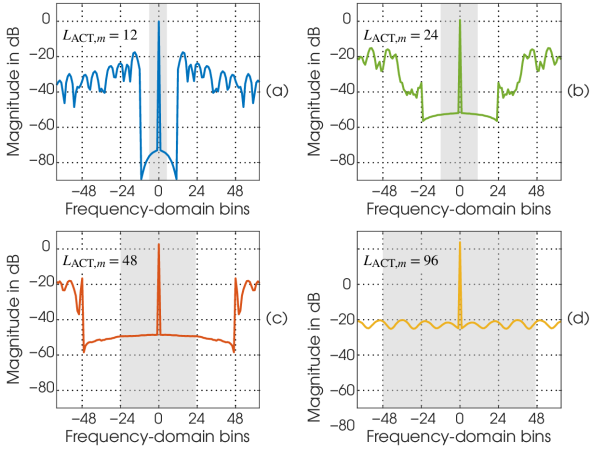
Figure 9: The FD representation of TD analysis window $\hat{\mathbf{a}}_{m}$ showing the distribution of significant coefficient values. Here, $L_{\text{OFDM},m}=128$ and the number of active subcarriers is (a) $L_{\text{ACT},m}=$12$$, (b) $L_{\text{ACT},m}=$24$$, (c) $L_{\text{ACT},m}=$48$$, and (d) $L_{\text{ACT},m}=$96$$. The grey-colored region in each sub-figure illustrates the bandwidth of the active subcarriers. As seen from this figure, the FD representation of the TD analysis filter is close to zero on $L_{\text{ACT},m}-1$ bins before and after the zero-frequency bin.

In the FD representations of the optimized analysis TD windows, the zero-frequency bin typically has the highest magnitude and other bins have significant values only for bins $[L_{\text{ACT},m}+1,L_{\text{ACT},m}+2,L_{\text{OFDM},m}-L_{\text{ACT},m}-2]$ as illustrated in Fig. 9. This is due to the fact that the FD kernel corresponding to analysis time-domain window should keep the signal on active subcarriers essentially intact. Therefore, these bins with possibility of having significant values are also selected as the optimization parameters. In this approach, the parameter vector $\boldsymbol{\phi}_{m}$ for the FD representation of the TD analysis window on subband $m$ is composed of zero-frequency bin as well as $L_{\text{OFDM},m}-2L_{\text{ACT},m}$ bins outside the active subcarriers. It is important to note that the proposed generalized FC processing with non-trivial TD windows inherently modifies the interpolation achieved by the FD zero-padding in OFDM modulation by properly weighting the interpolated samples to provide an interpolant with better spectral localization than using the straightforward rectangular analysis and synthesis TD windows.

The requirements for the FD representation of the TD analysis window can also be explained through convolution theorem. The element-wise multiplication of the time-domain CP-OFDM waveform by the time-domain analysis window is alternatively expressed by the circular convolution of the corresponding FD representations. Fig. 10 shows the FD representation of the TD analysis window and a rectangular window corresponding to allocation of $L_{\text{ACT},m}=12$ active subcarriers. In order to carry out the circular convolution such that the result has constant value over the active subcarriers, as shown by the line with square markers in Fig. 10, the FD representation of the TD analysis window has to be approximately zero in $L_{\text{ACT},m}-1$ bins on both sides of the zero-frequency bin.

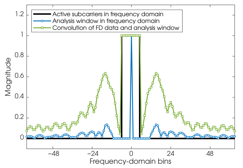
Figure 10: Illustration of the cyclic convolution of the rectangular window corresponding to waveform with bandwidth equal to $L_{\text{ACT},m}=12$ subcarriers by the frequency-domain representation of the TD analysis filter optimized for $L_{\text{ACT},m}=12$ active subcarriers.

It is assumed that all the windows are real valued and, therefore, when the analysis window length $L_{\text{OFDM},m}$ is even, first and $(L_{\text{OFDM},m}/2+1)$th bins of the corresponding FD representation are also real valued. The remaining bins, in general, have complex values such that the FD representation is conjugate symmetric with respect to $(L_{\text{OFDM},m}/2+1)$th bin and, therefore, both the real and imaginary parts of the corresponding coefficient values in the lower part of the conjugate-symmetric response need to be included in the optimization. Now, assuming that the $L_{\text{ACT},m}<L_{\text{OFDM},m}/2$, then the lower part of the FD representation of the TD analysis window can be constructed from the parameter vector $\boldsymbol{\phi}_{m}$ as follows

$$\alpha_{m}(0) =\phi_{m}(0)$$ (31)

$$\alpha_{m}(L_{\text{ACT},m}+p-1) =\phi_{m}(p)+$$

$$\mspace{20.0mu}{\mathop{\mspace{1.0mu}\mathrm{j}\mspace{0.5mu}}\nolimits}\phi_{m}(L_{\text{OFDM},m}/2-L_{\text{ACT},m}+1+p)$$

$$\alpha_{m}(L_{\text{OFDM},m}/2) =\phi_{m}(L_{\text{OFDM},m}/2-L_{\text{ACT},m}+1)$$

for $p=1,2,\dots,L_{\text{OFDM},m}/2-L_{\text{ACT},m}$. The corresponding upper part is obtained by taking the complex conjugate of the resulting lower part, expressed as

$$\alpha_{m}(L_{m}-n)=\operatorname{conj}(\alpha_{m}(n))$$ (32)

for $n=1,2,\dots,L_{m}/2-1$. Finally, the analysis window $\hat{\mathbf{a}}_{m}$ is obtained by taking the IDFT of the FD representation as follows:

$$\hat{\mathbf{a}}_{m}=\mathbf{W}^{-1}_{L_{\text{OFDM},m}}\boldsymbol{\alpha}_{m}.$$ (33)

For $L_{\text{ACT},m}\geq L_{\text{OFDM},m}/2$, the effect of time-domain analysis window becomes negligible due to the fact that the shape of the corresponding FD representation is already determined by $2L_{\text{ACT},m}$ zero-valued bins. Overall, this approach considerably reduces the number of parameters to be optimized especially for wider bandwidth allocations when compared with the straightforward parameterization of TD window values.

The TD synthesis window is parametrized in a same manner, however, now the synthesis window is, by definition, common for all the subbands and only the FD bins with indices $p=0,1,\dots,\gamma-1$ need to be taken into optimization. Here, $\gamma$ is a small integer, typically $520$ (see, Section V for details). Therefore, the lower part of the FD representation of the TD synthesis window can be constructed from the parameter vector $\boldsymbol{\psi}$ as follows

$$\beta(0)=\psi(0)\qquad\text{and}\qquad\beta(p)=\psi(p)+{\mathop{\mspace{1.0mu}\mathrm{j}\mspace{0.5mu}}\nolimits}\psi(\gamma+p)$$ (34)

for $p=1,2,\dots,\gamma-1$ and the upper part is obtained by taking the complex conjugate, expressed as

$$\beta(N-n)=\operatorname{conj}(\beta(n))$$ (35)

for $n=1,2,\dots,N/2-1$. Finally, the TD synthesis matrix is obtained by taking the IDFT of the FD representation, expressed as

$$\mathbf{S}=\operatorname{diag}(\mathbf{s})\quad\text{with}\quad\mathbf{s}=\mathbf{W}^{-1}_{N}\boldsymbol{\beta}.$$ (36)

III-C Transmultiplexer Optimization for Generalized FC-F-OFDM

The generalized FC-based F-OFDM system design can now be stated as an optimization problem for finding the optimal values of the aggregate parameter vector containing the adjustable parameters of all the windows as given by

$$\Xi=[\boldsymbol{\xi}_{0},\boldsymbol{\xi}_{1},\dots,\boldsymbol{\xi}_{M-1},\boldsymbol{\phi}_{0},\boldsymbol{\phi}_{1},\dots,\boldsymbol{\phi}_{M-1},\boldsymbol{\psi}]$$ (37a)

to

$$\underset{\Xi}{\text{minimize}} \max_{m=0,1,\dots,M-1}\left(\text{MSE}_{\text{AVG},m}\right)$$ (37b)

subject to $$\mathrm{SCR}_{m}\leq A_{\text{des}}\quad\text{for \,$m=0,1,\dots,M-1$},$$

where $A_{\text{des}}$ is the desired SCR target. The optimization problem in (37) can be straightforwardly solved using non-linear inequality constrained optimization algorithm, e.g., sequential quadratic programming [30]. Due to the non-convex nature of the problem and quite large number of optimization parameters, the convergence to the global optimum can not be unconditionally guaranteed. However, by using different starting points for the optimization, it can be shown that the algorithm converges reliably to same solution and, therefore, we can assume optimum is also the global one.

It should be noted that the goal here is not to reach the aperiodic convolution exactly through FC processing, instead, the optimization target is to keep the time-domain aliasing at a level that does not significantly impact the link error rate performance, such that the non-implementation-related effects are dominating. The main reason for MSE (or EVM) degradation is the loss of orthogonality due to the partial suppression of subcarriers, which is unavoidable in all filtered OFDM solutions. The proposed approach can be used for finding the desired trade-off between the frequency-selectivity of the processing and the resulting intrinsic interference of the filtering.

IV Implementation Complexity

The implementation complexity of the proposed generalized FC processing consist of forward and inverse FFTs and the TD and FD windowing. The number of real multiplications per FC processing block can be expressed as

$$C_{\text{M}}^{\text{(GFCB)}}=C_{\text{M}}^{\text{(TDSW)}}+C_{\text{M}}^{\text{(IFFT)}}+\sum_{m=0}^{M-1}C_{\text{M},m}^{\text{(TDAW)}}+C_{\text{M},m}^{\text{(FDW)}}+C_{\text{M},m}^{\text{(FFT)}},$$ (38)

where $C_{\text{M},m}^{\text{(TDAW)}}$’s, $C_{\text{M}}^{\text{(TDSW)}}$, and $C_{\text{M},m}^{\text{(FDW)}}$’s are, respectively, the number of real multiplications required for the TD analysis and synthesis windows as well as for the FD windows while $C_{\text{M},m}^{\text{(FFT)}}$’s and $C_{\text{M}}^{\text{(IFFT)}}$, respectively, are the number of real multiplications required for the FC short FFTs and long IFFT. The complexity of the OFDM processing consist of only IFFTs and can be expressed as

$$C_{\text{M}}^{\text{(OFDM)}}=\sum_{m=0}^{M-1}C_{\text{M},m}^{\text{(IFFT)}},$$ (39)

where $C_{\text{M},m}^{\text{(IFFT)}}$’s are the complexities of the OFDM IFFTs in terms of real multiplications. Now, the total number of real multiplications per CP-OFDM symbol can be expressed as

$$C_{\text{M}}=R_{m}C_{\text{M}}^{\text{(GFCB)}}/B_{\text{OFDM},m}+C_{\text{M}}^{\text{(OFDM)}},$$ (40)

where $R_{m}$, as given by (9), is the number of FC-processing blocks.

The number of real additions can be evaluated by replacing the $C_{\text{M},m}^{\text{(FFT)}}$’s, $C_{\text{M},m}^{\text{(IFFT)}}$’s, and $C_{\text{M}}^{\text{(IFFT)}}$ with the corresponding $C_{\text{A},m}^{\text{(FFT)}}$’s, $C_{\text{A},m}^{\text{(IFFT)}}$’s, and $C_{\text{A}}^{\text{(IFFT)}}$ giving the number of real additions required for the transforms and replacing the corresponding windowing complexities by zeros.

TABLE II: Number of real multiplications (muls) and additions (adds) for the FFT lengths of $N=\widehat{N}$ and $3\widehat{N}$ where $\widehat{N}$ is a power of two value.

	$N=\widehat{N}$	$N=3\widehat{N}$
Real muls	$C_{\text{M}}=\widehat{N}(\log_{2}(\widehat{N})-3)+4$	$C_{\text{M}}=\widehat{N}(3\log_{2}(\widehat{N})-7)+12$
Real adds	$C_{\text{A}}=\widehat{N}(3\log_{2}(\widehat{N})-3)+4$	$C_{\text{A}}=\widehat{N}(9\log_{2}(\widehat{N})+3)+12$

For a given transform length, the complexities of FFT and IFFT are, in general, the same. For power-of-two transform lengths, the split-radix algorithm is considered to be the most efficient one in terms of number of real multiplications [31] and the number of real multiplications and additions needed for the transforms are given in Table II. Here we consider also transform lengths of the form $3\widehat{N}$ where $\widehat{N}$ is a power-of-two value and the complexities are evaluated for prime-factor FFT [32]. Generally, the availability of transform lengths other than powers of two increases greatly the flexibility of waveform parametrization. The number of real multiplications and additions for the transform lengths to be considered later on are listed in Table III.

TABLE III: Number of real multiplications (muls) and additions (adds) per CP-OFDM symbol (or FC processing block) for some common transform lengths evaluated according to formulas in Table II

$N$	$16$	$24$	$32$	$48$	$64$	$128$
Real muls	$20$	$28$	$68$	$92$	$196$	$516$
Real adds	$148$	$252$	$388$	$636$	$964$	$2308$
$N$	$256$	$384$	$512$	$768$	$1024$	$2048$
Real muls	$1284$	$1804$	$3076$	$4364$	$7172$	$16\,388$
Real adds	$5380$	$8460$	$12\,292$	$19\,212$	$27\,652$	$61\,444$

TABLE IV: Example parametrizations for FC-F-OFDM-based 5G-NR physical layer with $20\text{\,}\mathrm{M}\mathrm{H}\mathrm{z}$ carrier bandwidth [28]

Config.	$f_{\text{SCS},m}$	$N_{\text{PRB},m}$	${L}_{\text{OFDM},m}$	${L}_{\text{CP},m}$	${f}_{\text{s},m}$	${L}_{m}$	${f}_{\text{s}}$
Narrow alloca- tion	$15\text{\,}\mathrm{k}\mathrm{H}\mathrm{z}$	$\leq$10$$	128	9	$1.92\text{\,}\mathrm{M}\mathrm{H}\mathrm{z}$	$N/16$	$30.72\text{\,}\mathrm{M}\mathrm{H}\mathrm{z}$
	$30\text{\,}\mathrm{k}\mathrm{H}\mathrm{z}$	$\leq$10$$	128	9	$3.84\text{\,}\mathrm{M}\mathrm{H}\mathrm{z}$	$N/8$	$30.72\text{\,}\mathrm{M}\mathrm{H}\mathrm{z}$
	$60\text{\,}\mathrm{k}\mathrm{H}\mathrm{z}$	$\leq$10$$	128	9	$7.68\text{\,}\mathrm{M}\mathrm{H}\mathrm{z}$	$N/4$	$30.72\text{\,}\mathrm{M}\mathrm{H}\mathrm{z}$
Config.	$f_{\text{SCS},m}$	$N_{\text{PRB},m}$	${L}_{\text{OFDM},m}$	${L}_{\text{CP},m}$	${f}_{\text{s},m}$	${L}_{m}$	${f}_{\text{s}}$
Wide alloca- tion	$15\text{\,}\mathrm{k}\mathrm{H}\mathrm{z}$	$\leq$106$$	2048	144	$30.72\text{\,}\mathrm{M}\mathrm{H}\mathrm{z}$	$N$	$30.72\text{\,}\mathrm{M}\mathrm{H}\mathrm{z}$
	$30\text{\,}\mathrm{k}\mathrm{H}\mathrm{z}$	$\leq$51$$	1024	72	$30.72\text{\,}\mathrm{M}\mathrm{H}\mathrm{z}$	$N$	$30.72\text{\,}\mathrm{M}\mathrm{H}\mathrm{z}$
	$60\text{\,}\mathrm{k}\mathrm{H}\mathrm{z}$	$\leq$24$$	512	36	$30.72\text{\,}\mathrm{M}\mathrm{H}\mathrm{z}$	$N$	$30.72\text{\,}\mathrm{M}\mathrm{H}\mathrm{z}$

V Application and Performance Evaluation in 5G-NR Physical Layer

In this section, we provide extensive numerical evaluations in the context of 3GPP 5G-NR mobile radio network which utilizes CP-OFDM as the baseline waveform. Following the 5G-NR specification, we assume that the active subcarriers on subband $m$ are always scheduled in PRBs of $12$ subcarriers [1], and thus $L_{\text{ACT},m}=12N_{\text{PRB},m}$, where $N_{\text{PRB},m}$ is the number of allocated PRBs in subband $m$. In the flexible physical layer numerology available in 5G-NR, the OFDM SCS is an integer power of two times $15\text{\,}\mathrm{k}\mathrm{H}\mathrm{z}$, that is, $f_{\text{SCS},m}=2^{\eta_{m}}\times$15\text{\,}\mathrm{k}\mathrm{H}\mathrm{z}$$ [4]. For an example carrier bandwidth of $20\text{\,}\mathrm{M}\mathrm{H}\mathrm{z}$, the sampling rate is $f_{\text{s}}=$30.72\text{\,}\mathrm{M}\mathrm{H}\mathrm{z}$$ with $N_{\text{OFDM},m}=2048/2^{\eta_{m}}$ and $N_{\text{CP},m}=144/2^{\eta_{m}}$. Since $L_{\text{CP},m}$, the CP length on the low-rate side, is constrained to be an integer, the minimum OFDM IFFT length becomes $L_{\text{OFDM},m}=$128$$. Now, for given maximum number of PRBs, the OFDM IFFT length can be determined as

$$L_{\text{OFDM},m}=\max\left\{2^{\xi_{m}},128\right\},$$ (41a)

where

$$\xi_{m}=\left\lceil\log_{2}(12N_{\text{PRB},m})\right\rceil.$$ (41b)

The FC processing transform sizes $N$ and $L_{m}$ are selected to achieve the desired interpolation factor.

Considering the mixed-numerology cases, $L_{m}$’s should be selected such that the associated $N$ becomes the same for all the numerologies. Table IV shows the example numerologies with OFDM SCSs of $15\text{\,}\mathrm{k}\mathrm{H}\mathrm{z}$, $30\text{\,}\mathrm{k}\mathrm{H}\mathrm{z}$, and $60\text{\,}\mathrm{k}\mathrm{H}\mathrm{z}$. By selecting the bin spacing in FC processing, as given by (21), to be larger than the SCS in OFDM processing, as given by (20), the complexity of the FC processing can be significantly reduced as shown later in this section. In addition, if the OFDM SCS and the FC bin spacing do not share a common factor, then increased flexibility is achievable in selecting the subband center frequencies. For example, by shifting the signal three bins to the right with $f_{\text{SCS},m}=$15\text{\,}\mathrm{k}\mathrm{H}\mathrm{z}$$ in OFDM processing domain and one bin to the left with $f_{\text{BS},m}=$40\text{\,}\mathrm{k}\mathrm{H}\mathrm{z}$$ bin spacing in FC processing domain, an overall shift of $5\text{\,}\mathrm{k}\mathrm{H}\mathrm{z}$ can be achieved if desired.

TABLE V: Passband MSEs in Example 1. FD window is adjustable in all cases. Here, $\lvert\Xi\rvert$ denotes the number of adjustable parameters in optimization

Case	TD	TD	MSE	MSE	$\lvert\Xi\rvert$	CPU
	synthesis	analysis	$(\lambda=\text{$\nicefrac{{1}}{{2}}$})$	$(\lambda=\text{$\nicefrac{{1}}{{4}}$})$		time
I			$-39.6\text{\,}\mathrm{d}\mathrm{B}$	$-31.5\text{\,}\mathrm{d}\mathrm{B}$	8	$120\text{\,}\mathrm{s}$
II	$\checkmark$		$-40.6\text{\,}\mathrm{d}\mathrm{B}$	$-31.5\text{\,}\mathrm{d}\mathrm{B}$	136	$1.5\text{\,}\mathrm{h}$
III		$\checkmark$	$-57.0\text{\,}\mathrm{d}\mathrm{B}$	$-40.4\text{\,}\mathrm{d}\mathrm{B}$	136	$0.8\text{\,}\mathrm{h}$
IV	$\checkmark$	$\checkmark$	$-58.4\text{\,}\mathrm{d}\mathrm{B}$	$-42.7\text{\,}\mathrm{d}\mathrm{B}$	264	$6.1\text{\,}\mathrm{h}$
V	$\checkmark$	$\checkmark$	$-56.6\text{\,}\mathrm{d}\mathrm{B}$	$-41.4\text{\,}\mathrm{d}\mathrm{B}$	131	$1.5\text{\,}\mathrm{h}$

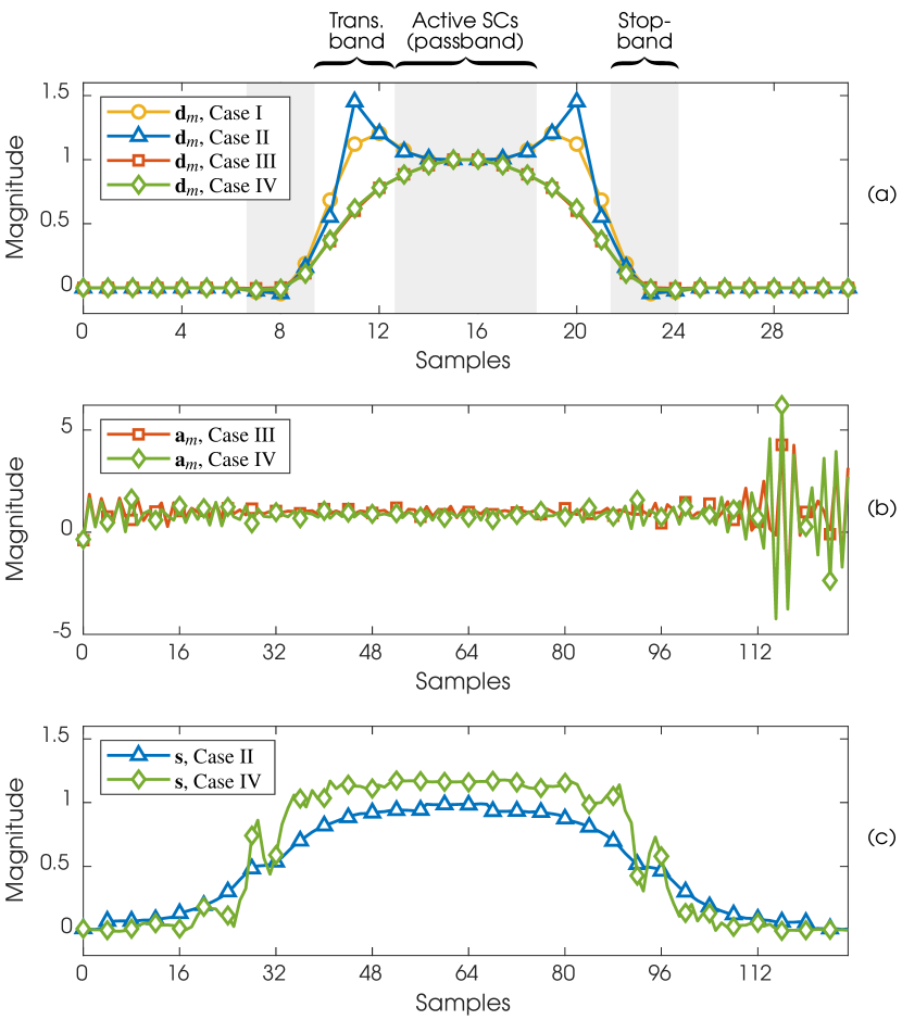
Figure 11: Optimized FD and TD windows in Example 1 with $50\text{\,}\%$ overlap. (a) FD windows. The passband and stopband regions with respect to FD windows are also illustrated in this figure. (b) Analysis TD windows. (c) Synthesis TD windows

V-A Example 1

Here we first compare the performance of the various FC processing alternatives by optimizing the windows in five cases shown in Table V. In this table, the check marks denote the windows which are adjustable in the optimization. Case I corresponds to the original FC processing in [13] with only adjustable FD window and Cases IV and V correspond to generalized processing where all the windows are adjustable. In Cases I–IV, all the values of the TD windows are adjustable as well as that of the FD window on passband and transition-band regions whereas in Case V, the parameter reduction techniques of Section III-B with $\gamma=20$ are utilized.

In this example, the number of subbands is $M=1$ while the number of active PRBs is $N_{\text{PRB},0}=2$ ($24$ active subcarriers), the OFDM IFFT length is $L_{\text{OFDM},0}=$128$$ while the FC FFT and IFFT lengths are $L_{0}=32$ and $N=4L_{0}=128$, respectively, corresponding to interpolation factor of $I_{0}=4$ and FC bin spacing of $f_{\text{BS},0}=4f_{\text{SCS},0}$. The desired SCR target is $A_{\text{des}}=$-50\text{\,}\mathrm{d}\mathrm{B}$$ and the overlap in FC processing is either $50\text{\,}\%$ or $25\text{\,}\%$ ($\lambda=0.5$ or $\lambda=0.25$).

The resulting passband MSE values are shown in Table V. As can be observed from these figures, the effect of TD synthesis window together with the FD window is negligible to MSE for both overlaps whereas the optimization of all the windows together reduces the MSE more than $15\text{\,}\mathrm{d}\mathrm{B}$ for the overlap of $50\text{\,}\%$ and more than $10\text{\,}\mathrm{d}\mathrm{B}$ for the overlap of $25\text{\,}\%$. However, since the synthesis window targets on smoothing the time-domain transients, this window mostly contributes on reducing the spectral leakage. It should be further pointed out that since the SCR target for the optimization is selected such that it can be met with plain FC processing, the full benefits of the synthesis window are not shown in this case. The optimized FD and TD windows are shown in Fig. 11 and, as seen from these responses, the optimized windows are not typical analytic window designs and, therefore, not feasible to devise without optimization techniques. In addition, these responses are different for all cases essentially meaning that the simultaneous optimization of all the windows is required for the best performance.

The number of variables in the optimization and the corresponding CPU times running Matlab R2018a on Intel Xeon E5-2620 are also given in Table V for reference. As seen from these optimization times, the parameter reduction techniques of Section III-B considerably reduces the optimization time with only slight degradation to MSE performance. However, for longer OFDM transform sizes, the computational complexity of the fully parameterized optimization increases dramatically. The optimization of FD window together with the TD analysis window allows in this particular case to reach faster essentially the same performance as in Case V with the reduced parameter set.

V-B Example 2

In this example, we evaluate the passband MSE performance of original and generalized FC-F-OFDM for different narrow-band configurations with $N_{\text{PRB},0}=\{1,2,4,8\}$ active PRBs (12, 24, 48, or 96 active subcarriers) and $15\text{\,}\mathrm{k}\mathrm{H}\mathrm{z}$ SCS for the OFDM processing. The purpose of this example is to more extensively compare the performance and the complexity of the original FC-F-OFDM processing with the proposed generalized one. In addition, the goal is to exemplify the effect of FC processing bin spacing to filtering performance and implementation complexity.

According to (41), the OFDM processing IFFT length can be selected as $L_{\text{OFDM},0}=128$. For sampling rate of $f_{\text{s}}=$30.72\text{\,}\mathrm{M}\mathrm{H}\mathrm{z}$$, the interpolation factor of $I_{0}=16$ is needed to achieve the desired overall symbol duration. Assuming that $f_{\text{BS},0}\geq f_{\text{SCS},0}$, then $L_{0}\leq L_{\text{OFDM},0}$ and $N=16L_{0}$. Here, we have chosen the FC short transform lengths of $L_{0}=\{16,24,32,48,64,128\}$ corresponding to FC processing bin spacings of $f_{\text{BS},0}=\{120,80,60,40,30,15\}$ kHz, respectively. The SCR targets in optimization are $A_{\text{des}}=\{$-40\text{\,}\mathrm{d}\mathrm{B}$,$-45\text{\,}\mathrm{d}\mathrm{B}$,$-50\text{\,}\mathrm{d}\mathrm{B}$,$-55\text{\,}\mathrm{d}\mathrm{B}$,$-60\text{\,}\mathrm{d}\mathrm{B}$,$-65\text{\,}\mathrm{d}\mathrm{B}$\}$ for transform lengths of $L_{0}=\{16,24,32,48,64,128\}$, respectively, and the overlap factor in FC processing is selected to be $50\text{\,}\%$. The number of transition band weights $L_{\text{TBW},0}$ is selected to cover $360\text{\,}\mathrm{k}\mathrm{H}\mathrm{z}$ bandwidth corresponding to $180\text{\,}\mathrm{k}\mathrm{H}\mathrm{z}$ guard band and $180\text{\,}\mathrm{k}\mathrm{H}\mathrm{z}$ measurement bandwidth, that is, $L_{\text{TBW},0}=\{3,5,6,9,12,24\}$ for $L_{0}=\{16,24,32,48,64,128\}$, respectively.

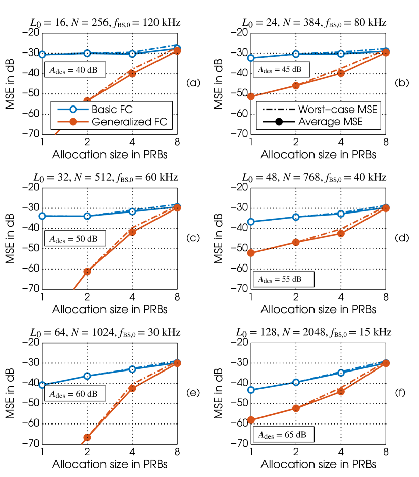
Figure 12: Average and worst-case passband MSEs for a filtered group of $N_{\text{PRB},0}=\{1,2,4,8\}$ PRBs with $50\text{\,}\%$ overlap in FC processing.

The results are shown in Figs. 12(a)–(f) for the given FC processing bin spacings. In these evaluations, the average and worst-case MSEs, as given by (27) and (28), are used as figure of merit of passband quality. The results are shown for both the proposed generalized processing and for the original FC processing in [13] (optimized and evaluated according to same criteria). We can see that both the worst-case and average MSEs are considerably better for the proposed generalized FC processing when compared to original scheme with only FD windowing. For both schemes, the worst-case MSE is slightly higher than the corresponding average. This is obviously due to the fact that on the edge subcarriers, the strict orthogonality is impaired. This contribution to average MSE is slightly higher with wider allocations. In addition, it can be observed that MSE errors increase as the allocation size increases. Furthermore, the difference in performance between these two schemes reduces for increasing allocation size. This is due to the fact that for wider allocations there are less interpolated samples (due to the FD zero padding in OFDM modulation) which can be used for controlling the spectral localization. Moreover, the processing where $L_{0}=3P$ with $P$ being the power of two has systematically higher MSE values for narrow allocations when compared with the power-of-two transform lengths. These results can be interpreted in the context of the EVM requirements of 5G-NR, stated as {$17.5\text{\,}\%$, $12.5\text{\,}\%$, $8\text{\,}\%$, $3.5\text{\,}\%$} or {$-15\text{\,}\mathrm{d}\mathrm{B}$, $-18\text{\,}\mathrm{d}\mathrm{B}$, $-22\text{\,}\mathrm{d}\mathrm{B}$, $-29\text{\,}\mathrm{d}\mathrm{B}$} for {QPSK, 16-QAM, 64-QAM, 256-QAM} modulations, respectively [28]. We can conclude that for 256-QAM, $120\text{\,}\mathrm{k}\mathrm{H}\mathrm{z}$ SCS can be considered sufficient from the average EVM point of view.

The implementation complexities of the original and proposed schemes are compared in Table VI. In this table, the figures annotated with asterisks correspond to original processing where the baseline FC processing bin spacing is the same as the OFDM processing SCS [13], while the complexities for the original processing with increased FC processing bin spacing are also given. The numbers typeset in bold face give the corresponding minimum complexities for the proposed scheme. It can be observed from this table that for the proposed scheme the number of real multiplications increases approximately $25\text{\,}\%$ or $40\text{\,}\%$ for the FC processing bin spacing of $15\text{\,}\mathrm{k}\mathrm{H}\mathrm{z}$ and $120\text{\,}\mathrm{k}\mathrm{H}\mathrm{z}$, respectively. However, overall, the complexity of the proposed processing with increased bin spacing is at least $15\text{\,}\%$ lower than that of the original with $15\text{\,}\mathrm{k}\mathrm{H}\mathrm{z}$ baseline processing [13].

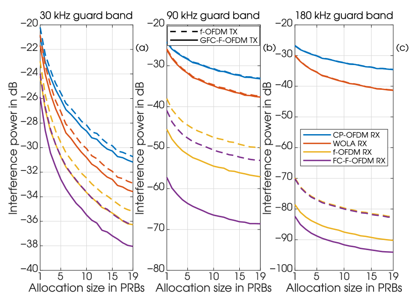
Figure 13: Inter-numerology interference (INI) seen by the victim RX averaged over the allocation size. On the TX side, either TD convolution-based f-OFDM or generalized FC-based F-OFDM processing is used while, on the RX side, plain CP-OFDM, WOLA, f-OFDM, or FC-F-OFDM is used. The guard band between the numerologies is (a) $30\text{\,}\mathrm{k}\mathrm{H}\mathrm{z}$, (b) $90\text{\,}\mathrm{k}\mathrm{H}\mathrm{z}$, or (c) $180\text{\,}\mathrm{k}\mathrm{H}\mathrm{z}$.

The complexities of the plain CP-OFDM, WOLA, and TD convolution-based f-OFDM are also included in Table VI. The overlapping extension in WOLA is assumed to be half the CP length ($72$ samples). For f-OFDM, the filter length is half the OFDM symbol length as defined in [8], that is, $N_{\text{FILT}}=N_{\text{OFDM}}/2$. Therefore, the overall complexity in terms of real multiplications per OFDM symbol is $C_{\text{M}}=N_{\text{FILT}}(N_{\text{OFDM}}+N_{\text{CP}})+C_{\text{M}}^{\text{(IFFT)}}$ when coefficient symmetry is utilized or $C_{\text{M}}=2N_{\text{FILT}}(N_{\text{OFDM}}+N_{\text{CP}})/I_{0}+C_{\text{M}}^{\text{(IFFT)}}$ when commutative model for the polyphase interpolator is used. As seen from this table, the complexity of the proposed processing scheme is approximately two times the complexity of CP-OFDM or WOLA and $1.42\text{\,}\%$ or $11.4\text{\,}\%$ that of the f-OFDM.

TABLE VI: Computational complexity of the proposed and original schemes for different numbers of processed CP-OFDM symbols and FC processing SCSs in Example 2. CP-OFDM, WOLA, and TD convolution-based f-OFDM (non-interpolating and interpolating processing) are shown here for reference.

$B_{\text{OFDM},0}$	$L_{\text{OFDM},0}$	$L_{\text{CP},0}$	$L_{0}$	$N$	$f_{\text{SCS},0}$	$f_{\text{BS},0}$	$C_{\text{M}}$	$C_{\text{M}}$	$N_{\text{OFDM}}$	$N_{\text{CP}}$	$C_{\text{M}}$	$C_{\text{M}}$	$C_{\text{M}}$
							(Original)	(Proposed)			(CP-OFDM)	(WOLA)	(f-OFDM)
1	128	9	128	2048	$15\text{\,}\mathrm{k}\mathrm{H}\mathrm{z}$	$15\text{\,}\mathrm{k}\mathrm{H}\mathrm{z}$	$68\,132$*	$84\,772$	2048	144	$16\,388$	$16\,676$	$2\,260\,996$
			16	256		$120\text{\,}\mathrm{k}\mathrm{H}\mathrm{z}$	$25\,292$	35 276					$280\,576$
7	128	9	128	2048	$15\text{\,}\mathrm{k}\mathrm{H}\mathrm{z}$	$15\text{\,}\mathrm{k}\mathrm{H}\mathrm{z}$	$39\,154$*	$48\,772$	2048	144	$16\,388$	$16\,676$	$2\,260\,996$
			16	256		$120\text{\,}\mathrm{k}\mathrm{H}\mathrm{z}$	$23\,057$	32 163					$280\,576$
14	128	9	128	2048	$15\text{\,}\mathrm{k}\mathrm{H}\mathrm{z}$	$15\text{\,}\mathrm{k}\mathrm{H}\mathrm{z}$	$37\,946$*	$47\,272$	2048	144	$16\,388$	$16\,676$	$2\,260\,996$
			16	256		$120\text{\,}\mathrm{k}\mathrm{H}\mathrm{z}$	$22\,963$	32 033					$280\,576$

The increased bin spacing in FC processing also reduces the overhead in short burst transmissions since the relative part of the time-domain zero padding (cf. (8)) with respect to the OFDM symbol length reduces. For example, with $f_{\text{BS},0}=$120\text{\,}\mathrm{k}\mathrm{H}\mathrm{z}$$ FC processing bin spacing, the number of output samples to be processed for one OFDM symbol is only $R_{0}N_{\text{S}}=20\times 128=2560$ which is half the samples required with $f_{\text{BS},0}=$15\text{\,}\mathrm{k}\mathrm{H}\mathrm{z}$$ bin spacing ($R_{0}N_{\text{S}}=5\times 1024=5120$). The latency of the processing is thus also reduced to half since the evaluation of the last samples corresponding to the current OFDM symbol is completed two times faster.

In order to further exemplify the performance of the generalized FC F-OFDM, while also comparing it against TD filtering-based approach, we consider the following scenario: Four PRBs with $30\text{\,}\mathrm{k}\mathrm{H}\mathrm{z}$ SCS are transmitted either using the generalized FC-based processing or TD convolution-based f-OFDM processing. The OFDM symbol length is $N_{\text{OFDM},0}=1024$ and CP length is $L_{\text{CP},0}=72$. The bin-spacing in the FC processing is $f_{\text{BS},0}=$15\text{\,}\mathrm{k}\mathrm{H}\mathrm{z}$$. Non-active allocation with $15\text{\,}\mathrm{k}\mathrm{H}\mathrm{z}$ SCS is located next to active allocation such that the guard band between the allocations is either $30\text{\,}\mathrm{k}\mathrm{H}\mathrm{z}$, $90\text{\,}\mathrm{k}\mathrm{H}\mathrm{z}$, or $180\text{\,}\mathrm{k}\mathrm{H}\mathrm{z}$. The bandwidth of the non-active allocation is adjusted from $1$ PRB to $19$ PRBs. On the RX side, either plain CP-OFDM, WOLA, f-OFDM, or FC filtered-OFDM is used. In the optimization, the objective function and the constraints are now interchanged such that the SCR is minimized subject to constraint that in-band MSE has to be at least $-37.0\text{\,}\mathrm{d}\mathrm{B}$. Fig. 13 shows the interference power evaluated over the non-active subcarriers for each TX/RX processing alternative. As seen from this figure, generalized FC-based TX processing has considerably better performance when compared with f-OFDM TX while f-OFDM RX can also be used with generalized FC-based TX processing. Overall, the results in Fig. 13 clearly illustrate the excellent bandlimitation properties of the generalized FC based transmitter processing.

V-C Example 3

Here, we consider a wideband example where the FC processing carries out the channelization filtering of an overall $5\text{\,}\mathrm{M}\mathrm{H}\mathrm{z}$ OFDM carrier with $n_{\text{ACT}}=300$ active subcarriers ($N_{\text{PRB},0}=25$) and sampling rate of $f_{\text{s}}=$7.68\text{\,}\mathrm{M}\mathrm{H}\mathrm{z}$$ and at the same time the signal is interpolated to the output rate of $122.88\text{\,}\mathrm{M}\mathrm{H}\mathrm{z}$. Now, the OFDM processing IFFT length has to be at least $L_{\text{OFDM},0}=512$ according to (41). Assuming that the FC BS is chosen as $f_{\text{BS},0}=2f_{\text{SCS},0}=$30\text{\,}\mathrm{k}\mathrm{H}\mathrm{z}$$, the FC transform sizes are $L_{0}=256$ and $N=4096$. The average and worst-case MSE values for the original and generalized FC processing are shown in Table VII. As seen from this table, the generalized model only slightly improves the performance with respect to original processing for the case when the allocation size is larger than the OFDM IFFT size divided by two.

If the OFDM IFFT size is increased to $L_{\text{OFDM},0}=1024$ and FC processing inverse transform size is reduced to $N=2048$ while keeping $L_{\text{OFDM},0}=512$, then the proposed generalized model achieves more than $5\text{\,}\mathrm{d}\mathrm{B}$ better average MSE when compared to the original scheme with same parameterization and $9\text{\,}\mathrm{d}\mathrm{B}$ improvement when compared to original FC-F-OFDM scheme with OFDM IFFT size of $L_{\text{OFDM},0}=512$. These improved MSE values are indicated in bold typeface in Tab. VII.

TABLE VII: Passband MSEs in Example 3.

	${L}_{\text{OFDM},0}=512$, ${L}_{0}=256$, and $N=4096$		${L}_{\text{OFDM},0}=1024$, ${L}_{0}=256$, and $N=2048$
	Original	Proposed	Original	Proposed
$\text{MSE}_{\text{AVG},0}$	$-33.9\text{\,}\mathrm{d}\mathrm{B}$	$-34.3\text{\,}\mathrm{d}\mathrm{B}$	$-37.3\text{\,}\mathrm{d}\mathrm{B}$	$42.9\text{\,}\mathrm{d}\mathrm{B}$
$\text{MSE}_{\text{MAX},0}$	$-30.1\text{\,}\mathrm{d}\mathrm{B}$	$-31.7\text{\,}\mathrm{d}\mathrm{B}$	$-31.7\text{\,}\mathrm{d}\mathrm{B}$	$34.8\text{\,}\mathrm{d}\mathrm{B}$

V-D Example 4

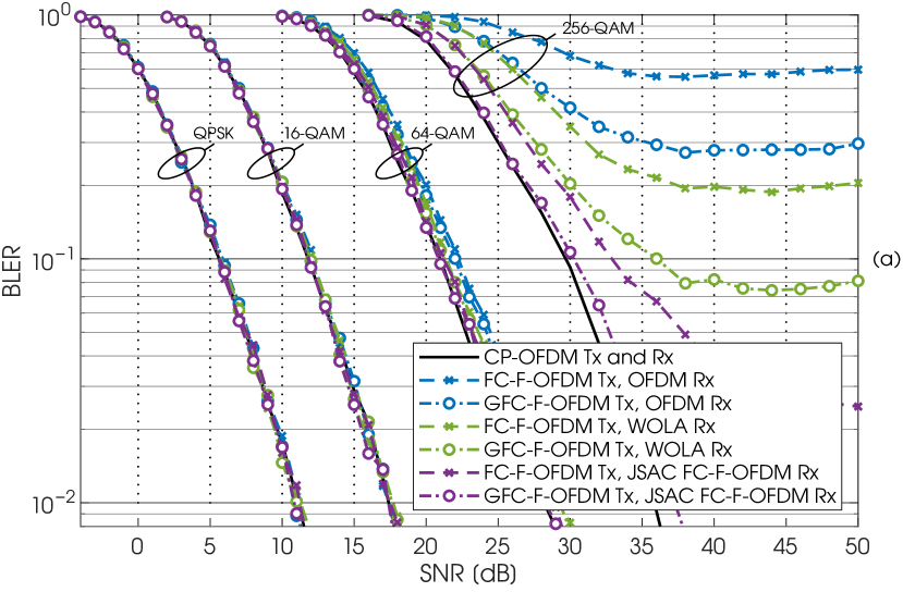
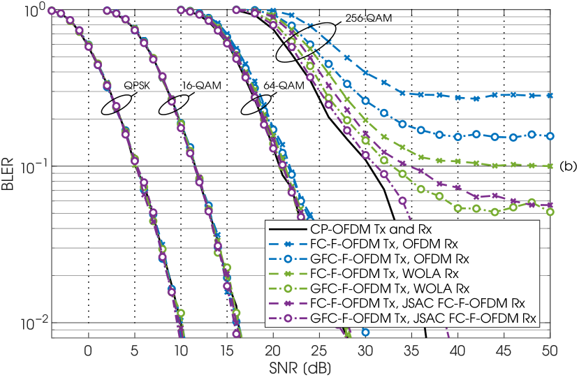
Figure 14: Block error rate without CFO in downlink mixed numerology interference scenario with (a) 1 PRB and (b) 4 PRB allocation for the desired signal with 1 PRB guard band between the signals. The desired signal is assumed to use $15\text{\,}\mathrm{k}\mathrm{H}\mathrm{z}$ SCS and the interfering signal is assumed to use $30\text{\,}\mathrm{k}\mathrm{H}\mathrm{z}$ SCS. CP-OFDM curves refer to ideal reference case with desired signal only.

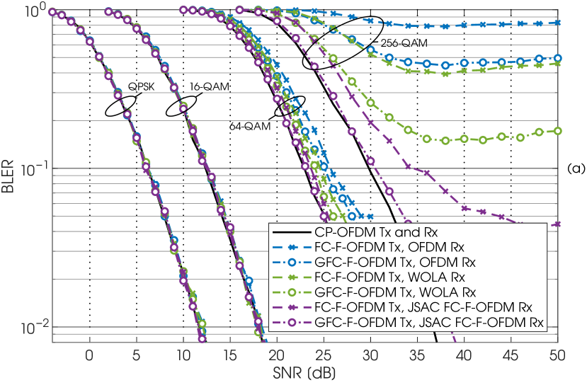
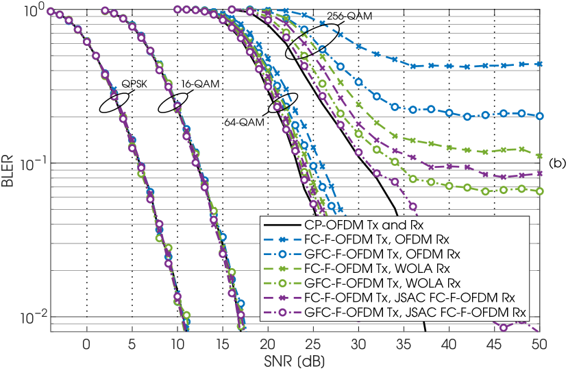
Figure 15: Block error rate with CFO in downlink mixed numerology interference scenario with (a) 1 PRB and (b) 4 PRB allocation for the desired signal with 1 PRB guard band between the signals. The desired signal is assumed to use $15\text{\,}\mathrm{k}\mathrm{H}\mathrm{z}$ SCS and the interfering signal is assumed to use $30\text{\,}\mathrm{k}\mathrm{H}\mathrm{z}$ SCS. CP-OFDM curves refer to ideal reference case with desired signal only.

In this final example, the actual downlink (DL) mixed-numerology radio link performance is evaluated in terms of coded block error rate (BLER). We assume that $f_{\text{BS},m}=$120\text{\,}\mathrm{k}\mathrm{H}\mathrm{z}$$ is used in both the original and generalized FC processing on the TX side. This corresponds to the scenario presented in Fig. 12(a), which allows to minimize the complexity and the latency of the FC processing as indicated in Table VI. On the RX side either plain CP-OFDM receiver, WOLA [7, 11] based RX waveform processing, or original FC-F-OFDM-based receiver waveform processing [13] is applied. With WOLA, a rising or falling window slope length of $L_{\text{CP},m}/4$ samples with $m=0,1$ is assumed and the slope follows the well known raised-cosine response. With original FC-F-OFDM RX operating with $15\text{\,}\mathrm{k}\mathrm{H}\mathrm{z}$ bin spacing, we have used the filter design presented in [13] to optimize RX FD window with $12$ transition-band bins and $10\text{\,}\mathrm{d}\mathrm{B}$ attenuation target.

The radio link performance of the desired CP-OFDM signal with $f_{\text{SCS},0}=$15\text{\,}\mathrm{k}\mathrm{H}\mathrm{z}$$ and with either 1 PRB or 4 PRB allocation is measured while being interfered from one side by another CP-OFDM signal with $f_{\text{SCS},1}=$30\text{\,}\mathrm{k}\mathrm{H}\mathrm{z}$$ and with a fixed 4 PRB allocation. The guard band between the two different numerologies is assumed to be $180\text{\,}\mathrm{k}\mathrm{H}\mathrm{z}$, following the earlier discussion. As we are modeling DL mixed numerology interference, it is assumed that the base station transmitter applies the same waveform processing on both transmitted signals. The evaluated modulations correspond to QPSK, 16- quadrature amplitude modulation (QAM), 64-QAM, and 256-QAM with coding rates $R=602/1024$, $R=658/1024$, $R=873/1024$, and $R=885/1024$, respectively. These correspond to modulation and coding scheme (MCS) indices 4, 10, 19, and 25 in the MCS index Table 2 defined in [33, Table 5.1.3.1-2]. A wide range of evaluated MCSs allows to understand which modulations are sensitive to the MSE levels induced by considered TX processing solutions and also highlight how different RX processing solutions affect the performance. In addition, 256-QAM modulation based operation point is included to illustrate how generalized FC processing allows us to use high MCS even with narrow allocations and minimal complexity increase compared to original FC processing. The assumed slot length for both subband signals is $14$ OFDM symbols and the performance is averaged over $5000$ independent channel realizations. The assumed radio propagation model is a tapped-delay line (TDL) C channel [34] with $300\text{\,}\mathrm{n}\mathrm{s}$ root-mean-squared delay spread. The evaluations are based on a 5G-NR compliant link simulator.

In Fig. 14, illustrating the link performance without carrier frequency offset (CFO), the relatively small MSE induced by the subband filtering does not have significant effect with modulation orders smaller than 256-QAM. With 64-QAM, approximately $2\text{\,}\mathrm{d}\mathrm{B}$ difference in the required signal-to-noise ratio (SNR) for $\text{BLER}=10^{-1}$ is observed when comparing plain OFDM RX performance to WOLA or FC-F-OFDM-based RX performance. This difference is mainly from the assumed RX processing. In the case of 256-QAM, the effect of using generalized FC or original FC processing in the TX is more clearly visible, and the error floor behaviour with generalized FC TX processing is defined by the considered RX waveform processing solution. The CP-OFDM-based RX collects interference from neighboring subband and therefore provides the worst performance in all cases. With WOLA-based RX, the performance is clearly improved, but due to the limited selectivity the performance is not as good as with FC-based RX. As expected, lower order modulations are not as sensitive to TX MSE induced by the subband filtering, whereas with 256-QAM clear differences can be observed. The RX waveform processing has a significant impact on the link performance, although highly selective and low in-band distortion enabling generalized FC processing is applied in TX. Another way to look at these results, is to note that using generalized FC-based TX processing allows the best possible performance from the TX side, and the experienced link performance depends on the RX implementation, which can be improved in the future device generations if highly selective subband filtering is applied in the devices. Based on Fig. 13, it can also be presumed that the effect of filtering becomes more profound when the guard band between numerologies is reduced from $180\text{\,}\mathrm{k}\mathrm{H}\mathrm{z}$ and that the effect becomes visible also with lower modulation orders.

To highlight the possible effect of CFO on the DL link performance, results with CFO are shown in Fig. 15. As we are concentrating on DL performance, the CFO between the base station and the user equipment affects both subbands similarly. Thus, the receiving device observes the same frequency offset in the desired signal and in the interfering signal. In these evaluations, we have assumed a $350\text{\,}\mathrm{H}\mathrm{z}$ CFO, corresponding to the 0.1 part-per-million ($0.1\text{\,}\mathrm{p}\mathrm{p}\mathrm{m}$) accuracy required from the base station transmitter, as defined in [28], while noting that the performance evaluations are done at the $3.5\text{\,}\mathrm{G}\mathrm{H}\mathrm{z}$ carrier frequency. Based on the results shown in Fig. 15, we can observe that with 64-QAM, CP-OFDM RX, WOLA RX, and FC-F-OFDM RX require approximately $2.5\text{\,}\mathrm{d}\mathrm{B}$, $1.5\text{\,}\mathrm{d}\mathrm{B}$, and $0.5\text{\,}\mathrm{d}\mathrm{B}$ larger SNR at $10\text{\,}\%$ BLER target level, respectively, when using FC-F-OFDM TX, and $2\text{\,}\mathrm{d}\mathrm{B}$, $1\text{\,}\mathrm{d}\mathrm{B}$, and $0.1\text{\,}\mathrm{d}\mathrm{B}$ larger SNR at $10\text{\,}\%$ BLER target level, respectively, when using GFC-F-OFDM TX. It is noted that with 256-QAM, due to its larger sensitivity to CFO [35], we have applied a demodulation reference signals (DMRS)-based fine-frequency tracking in the receiver. From Fig. 15 (a), we can observe that in the case of 1 PRB allocation, FC-based RX processing is required to support 256-QAM modulation, and with generalized FC-based TX the performance is very close to the interference free reference. In the case of 4 PRBs, as shown in Fig. 15 (b), it is interesting to note that by applying generalized FC processing on the TX side, we are able to support 256-QAM modulation also with WOLA-based RX. Comparing the 256-QAM results shown in Fig. 15 with Fig. 14, we can observe that the clear in-band MSE improvement provided by the genralized FC TX processing is maintained also under CFO. Generalized FC processing is thus shown to be the most efficient processing solution to flexibly allocate different numerologies with only $180\text{\,}\mathrm{k}\mathrm{H}\mathrm{z}$ guard band apart from each other while simultaneously supporting full range of different MCS values currently defined in the 5G-NR specifications and allowing more degrees of freedom in the implementation.

VI Conclusions

In this article, focusing on non-orthogonal multiple-access scenarios with CP-OFDM waveform, we presented a novel spectrum enhancement method combining analysis and synthesis time-domain windowing with subband filtering implemented through the fast-convolution process. It was found that joint optimization of the time- and frequency-domain windows can offer greatly enhanced performance over basic subband filtering, and also over straightforward combinations of filtering and time-domain windowing. This conclusion was verified also by detailed link-level simulations in typical 5G-NR downlink mixed-numerology scenarios. The performance gain over original FC-F-OFDM is pronounced with relatively narrow allocations using modulation and coding schemes aiming at high spectral efficiency. Generally, the demonstrated performance gains help to enhance the spectrum utilization efficiency of CP-OFDM-based multiservice wireless networks, like the emerging 5G-NR. In this article, we also extended the parametrization alternatives of original and generalized FC-F-OFDM by considering independent choice of the subcarrier spacing and the FFT bin spacing in FC processing. This was found to support feasible performance with greatly reduced complexity and processing latency, providing additional degrees of freedom in the design and implementation.

Strong emphasis in this work was on the transparent spectrum enhancement schemes, which allows fast initial deployment and backwards compatible enhancements of 5G-NR technology. The proposed scheme was applied for the transmitter side of the link, while plain CP-OFDM receiver was assumed in the joint optimization of the time- and frequency domain window coefficients. Throughout the different examples, the received signal quality and link performance were shown to improve with different transparent receiver waveform processing solutions when generalized FC-F-OFDM was applied in the transmitter. However, the idea of combined joinly-optimized time- and frequency-domain windowing can be applied on the receiver side as well. Therefore, the optimization of receiver-side processing in transparent way, and joint transmitter-receiver optimization using time- and frequency-domain windows will be the main topics for our future studies.

Juha Yli-Kaakinen received the degree of Diploma Engineer in electrical engineering and the Doctor of Technology (Hons.) degree from the Tampere University of Technology (TUT), Tampere, Finland, in 1998 and 2002, respectively. Since 1995, he has held various research positions with TUT. His research interests are in digital signal processing, especially in digital filter and filter-bank optimization for communication systems and very large scale integration implementations.

Toni Levanen received the M.Sc. and D.Sc. degrees from Tampere University of Technology (TUT), Finland, in 2007 and 2014, respectively. He is currently with the Department of Electrical Engineering, Tampere University. In addition to his contributions in academic research, he has worked in industry on wide variety of development and research projects. His current research interests include physical layer design for 5G NR, interference modelling in 5G cells, and high-mobility support in millimeter-wave communications.

Arto Palin has long industrial experience in wireless technologies, covering cellular networks, broadcast systems and local area communications. He holds an MSc. (Tech.) degree from earlier Tampere University of Technology, and is currently working as Technical Leader at Nokia Mobile Networks, Finland, in the area of 5G SoC architectures.

Markku Renfors (S’77–M’82–SM’90–F’08) received the D.Tech. degree from the Tampere University of Technology (TUT), Tampere, Finland, in 1982. Since 1992, he has been a Professor with the Department of Electronics and Communications Engineering, TUT, where he was the Head from 1992 to 2010. His research interests include filter-bank based multicarrier systems and signal processing algorithms for flexible communications receivers and transmitters. Dr. Renfors was a corecipient of the Guillemin Cauer Award (together with T. Saramäki) from the IEEE Circuits and Systems Society in 1987.

Mikko Valkama received the D.Sc. (Tech.) degree (with honors) from Tampere University of Technology, Finland, in 2001. In 2003, he was with the Communications Systems and Signal Processing Institute at SDSU, San Diego, CA, as a visiting research fellow. Currently, he is a Full Professor and Department Head of Electrical Engineering at newly formed Tampere University (TAU), Finland. His general research interests include radio communications, radio localization, and radio-based sensing, with particular emphasis on 5G and beyond mobile radio networks.

References

- [1] E. Dahlman, S. Parkvall, and J. Skold, 5G NR: The Next Generation Wireless Access Technology. Academic Press, 2018.
- [2] G. Wunder, P. Jung et al., “5GNOW: Non-orthogonal, asynchronous waveforms for future mobile applications,” IEEE Commun. Mag., vol. 52, no. 2, pp. 97–105, Feb. 2014.
- [3] P. Banelli, S. Buzzi et al., “Modulation Formats and Waveforms for 5G Networks: Who Will Be the Heir of OFDM?: An overview of alternative modulation schemes for improved spectral efficiency,” IEEE Signal Processing Mag., vol. 31, no. 6, pp. 80–93, Nov. 2014.
- [4] Technical Specification Group Radio Access Network, NR; NR and NG-RAN Overall Description; Stage 2 (Release 15), document TS 38.300 V15.7.0, 3GPP, Sep. 2019.
- [5] Technical Specification Group Radio Access Network; Study on New Radio Access Technology Physical Layer Aspects (Release 14), document TR 38.802 V14.2.0, 3GPP, Sep. 2017.
- [6] T. Levanen, J. Pirskanen et al., “Transparent Tx and Rx waveform processing for 5G new radio mobile communications,” IEEE Wireless Commun., vol. 26, no. 1, pp. 128–136, Feb. 2019.
- [7] H. Wang, Y. Lu, and X. Wang, “Channelized receiver with WOLA filterbank,” in Proc. CIE Int. Conf. Radar, Oct. 2006, pp. 1–3.
- [8] X. Zhang, M. Jia et al., “Filtered-OFDM – Enabler for flexible waveform in the 5th generation cellular networks,” in Proc. IEEE Global Commun. Conf. (GLOBECOM), Dec. 2015, pp. 1–6.
- [9] R. Ahmed, T. Wild, and F. Schaich, “Coexistence of UF-OFDM and CP-OFDM,” in Proc. IEEE Veh. Techn. Conf. (VTC Spring), May 2016, pp. 1–5.
- [10] J. Luo, A. Zaidi et al., “Preliminary radio interface concepts for mm-wave mobile communications,” Project mmMACIG (Millimetre-Wave Based Mobile Radio Access Network for Fifth Generation Integrated Communications) Technical Report D4.1, Jan. 2016.
- [11] R. Zayani, Y. Medjahdi et al., “WOLA-OFDM: A potential candidate for asynchronous 5G,” in Proc. IEEE Globecom Workshops (GC Wkshps), Dec. 2016, pp. 1–5.
- [12] L. Zhang, A. Ijaz et al., “Filtered OFDM systems, algorithms, and performance analysis for 5G and beyond,” IEEE Trans. Commun., vol. 66, no. 3, pp. 1205–1218, Mar. 2018.
- [13] J. Yli-Kaakinen, T. Levanen et al., “Efficient fast-convolution-based waveform processing for 5G physical layer,” IEEE J. Sel. Areas Commun., vol. 35, no. 6, pp. 1309–1326, June 2017.
- [14] J. Li, E. Bala, and R. Yang, “Resource block filtered-OFDM for future spectrally agile and power efficient systems,” Physical Communication, vol. 14, pp. 36–55, Jun. 2014.
- [15] M. Renfors, J. Yli-Kaakinen et al., “Efficient fast-convolution implementation of filtered CP-OFDM waveform processing for 5G,” in Proc. IEEE Globecom Workshops, San Diego, CA, USA, Dec. 2015.
- [16] ——, “Fast-convolution filtered OFDM waveforms with adjustable CP length,” in Proc. IEEE Global Conf. Signal Inform. Process. (GlobalSIP), Greater Washington, D.C., USA, Dec. 7–9 2016, pp. 635–639.
- [17] B. Hunt, “A matrix theory proof of the discrete convolution theorem,” IEEE Trans. Audio Electroacoust., vol. 19, no. 4, pp. 285–288, Dec. 1971.
- [18] L. R. Rabiner and B. Gold, Theory and Application of Digital Signal Processing. Englewood Cliffs, NJ: Prentice-Hall, 1975.
- [19] C. C. Kwan, “Digital signal processing techniques for on-board processing satellites,” Ph.D. dissertation, University of Surrey, Guildford, United Kingdom, 1990.
- [20] M.-L. Boucheret, I. Mortensen, and H. Favaro, “Fast convolution filter banks for satellite payloads with on-board processing,” IEEE J. Select. Areas Commun., vol. 17, no. 2, pp. 238–248, Feb. 1999.
- [21] C. Zhang and Z. Wang, “A fast frequency domain filter bank realization algorithm,” in Proc. Int. Conf. Signal Processing (ICSP), vol. 1, Beijing, China, Aug. 21–25 2000, pp. 130–132.
- [22] L. Pucker, “Channelization techniques for software defined radio,” in Proc. Software Defined Radio Technical Conf. (SDR), Orlando, FL, USA, Nov. 18–19 2003.
- [23] M. Renfors, J. Yli-Kaakinen, and F. Harris, “Analysis and design of efficient and flexible fast-convolution based multirate filter banks,” IEEE Trans. Signal Processing, vol. 62, no. 15, pp. 3768–3783, Aug. 2014.
- [24] J. Yli-Kaakinen and M. Renfors, “Optimization of flexible filter banks based on fast convolution,” Journal of Signal Processing Systems, vol. 85, no. 1, pp. 101–111, Aug. 2016.
- [25] K. Shao, J. Alhava et al., “Fast-convolution implementation of filter bank multicarrier waveform processing,” in Proc. IEEE Int. Symp. on Circuits and Systems (ISCAS), Lisbon, Portugal, May 24–27 2015, pp. 978–981.
- [26] M. Renfors and J. Yli-Kaakinen, “Flexible fast-convolution implementation of single-carrier waveform processing,” in Proc. IEEE Int. Conf. Commun. Workshops (ICCW), London, UK, Jun. 8–12 2015, pp. 1243–1248.
- [27] Technical Specification Group Radio Access Network; NR; Physical Channels and Modulation (Release 15), document TS 38.211 V15.6.0, 3GPP, Jun. 2019.
- [28] Technical Specification Group Radio Access Network; NR; Base Station (BS) Radio Transmission and Reception (Release 15), document TS 38.104 V16.0.0, 3GPP, Jun. 2019.
- [29] Technical Specification Group Radio Access Network; Study on new radio access technology: Radio Frequency (RF) and co-existence aspects (Release 14), document TR 38.803 V14.2.0, 3GPP, Sep. 2017.
- [30] J. Nocedal and S. J. Wright, Numerical Optimization. Springer, 2006.
- [31] H. Sorensen, M. Heideman, and C. Burrus, “On computing the split-radix FFT,” IEEE Trans. Acoust., Speech, Signal Process., vol. 34, no. 1, pp. 152–156, Feb. 1986.
- [32] D. Kolba and T. Parks, “A prime factor FFT algorithm using high-speed convolution,” IEEE Trans. Acoust., Speech, Signal Process., vol. 25, no. 4, pp. 281–294, Aug 1977.
- [33] Technical Specification Group Radio Access Network; NR; Physical layer procedures for data (Release 15), document TS 38.214 V15.6.0, 3GPP, Jun. 2019.
- [34] Technical Specification Group Radio Access Network; Study on channel model for frequency spectrum above 6 GHz (Release 15), document TR 38.900 V15.0.0, 3GPP, Jun. 2018.
- [35] T. Pollet, M. Van Bladel, and M. Moeneclaey, “BER sensitivity of OFDM systems to carrier frequency offset and Wiener phase noise,” IEEE Trans. Commun., vol. 43, no. 2/3/4, pp. 191–193, Feb 1995.