Surface van der Waals Forces in a Nutshell

Abstract

Most often in chemical physics, long range van der Waals surface interactions are approximated by the exact asymptotic result at vanishing distance, the well known additive approximation of London dispersion forces due to Hamaker. However, the description of retardation effects that is known since the time of Casimir is completely neglected for lack of a tractable expression. Here we show that it is possible to describe surface van der Waals forces at arbitrary distances in one single simple equation. The result captures the long sought crossover from non-retarded (London) to retarded (Casimir) interactions, the effect of polarization in condensed media and the full suppression of retarded interactions at large distance. This is achieved with similar accuracy and the same material properties that are used to approximate the Hamaker constant in conventional applications. The results show that at ambient temperature, retardation effects significantly change the power law exponent of the conventional Hamaker result for distances of just a few nanometers.

Van der Waals interactions are at the heart of chemical physics. Yet, the standard textbook answer on their essential charcteristic is the well known inverse sixth power dependence on the distance. This is a largely biased statement towards the London picture of molecular interactions, which treats intermolecular forces as a result of classical electrodynamic fluctuations. At distances of just a few nanometers, molecular interactions develop a different, faster decay that results from purely quantum electrodynamic fluctuations and was first described in the seminal work of Casimir (c.f. Power, 2001 and Lamoreaux, 2007 for a hystorical perspective).

An aclaimed unification of these two complementary views on the range of molecular interactions has been known for a long time.Dzyaloshinskii et al. (1961) The Dzyaloshinskii-Lifshitz-Pitaevskii theory (DLP) for surface forces accross a medium is the solution of the full thermal quantum electrodynamic field theory for the forces between two plates across a dielectric continuum. As a result, it generalizes in one single equation the Hamaker theory of additive dispersive forces, the Debye induction potential between polar and polarizable media, and the Keesom interactions between Boltzmann distributed dipoles. It describes the cross–over from purely non-retarded dispersive to retarded long–range interactions, it reduces to the Casimir-Polder formula for the retarded force between metallic plates in vacuum, and provides the famous result of London for the dispersion interaction between two atoms at short distances.

Not surprisingly, the theory has had a profound impact on fundamental physics,Lamoreaux (2007) it has motivated a large number of historical experiments,Tabor and Winterton (1969); Israelachvili and Tabor (1972); Sabisky and Anderson (1973); Bevan and Prieve (1999); Mohideen and Roy (1998); Munday et al. (2009) and retains its theoretical influence in promising new studies up to date.Berthoumieux and Maggs (2010); Berthoumieux (2018)

Unfotunately, with some exceptions the general theory of van der Waals interactions is largely ignored in favor of the Hamaker picture of additive dispersive forces.Israelachvili (1991) The reason is simple to infer, as the power and generality of this approach comes at the cost of a complicated and lengthy formula that can hardly be interpreted qualitatively, except in special limiting cases after lengthy manipulations and detailed knowledge on materials properties.Safran (1994); Parsegian (2006); Ninham and Nostro (2010); Butt and Kappl (2010); French et al. (2010)

Here, we show that the theory of surface van der Waals forces can be formulated as one single simple equation that embodies simultaneously the known low and high temperature limits, the crossover from retarded to non retarded interactions and the far less appreciated long range exponential suppression of retardation effects. The result allows us to interpret easily the main qualitative features of van der Waals forces for arbitrary distances and provides a convenient means to compute quantitatively the results in analytic form.

The surface free energy between two semi-infinite macroscopic bodies, 1 and 2, separated by a third body, $m$, of thickness $L$, may be written in terms of the effective Hamaker function, $A(L)$, as $g(L)=-\frac{A(L)}{12\pi L^{2}}$. In practice, $A(L)$ is a constant at small separations only, and develops a complicated $L$ dependence that is given in DLP theory as:

$$A(L)=\frac{3}{2}k_{B}T\sum_{n=0}^{\infty}\,{}^{\prime}\int_{r_{n}}^{\infty}x[R^{M}_{1m2}(x,n)+R^{E}_{1m2}(x,n)]e^{-x}dx$$ (1)

where $R^{M}_{1m2}(x,n)=\Delta^{M}_{1m}(x,n)\Delta^{M}_{2m}(x,n)$, $R^{E}_{1m2}(x,n)=\Delta^{E}_{1m}(x,n)\Delta^{E}_{2m}(x,n)$, while

$$\begin{array}[]{lcl}\Delta^{M}_{ij}=\frac{x_{i}\epsilon_{j}-x_{j}\epsilon_{i}}{x_{i}\epsilon_{j}+x_{j}\epsilon_{i}}&&\Delta^{E}_{ij}=\frac{x_{i}-x_{j}}{x_{i}+x_{j}}\end{array}$$ (2)

and $x_{i}^{2}=x^{2}+(\epsilon_{i}-\epsilon_{m})(2\omega_{n}L/c)^{2}$. In these equations, the prime next to the sum implies that the $n=0$ term has an extra factor of $1/2$. The dielectric function, $\epsilon_{i}$, is evaluated at the imaginary angular frequencies $i\omega_{n}$, where $\omega_{n}=\omega_{T}n$ are integer multiples of the thermal Matsubara frequency $\omega_{T}=\frac{2\pi k_{B}T}{\hbar}$. The magnetic permitivities have been assumed equal to unity. The lower integration limit is $r_{n}=2\epsilon_{m}^{1/2}\omega_{n}L/c$; while $k_{B}$ and $\hbar$, $c$ are the usual fundamental constants. Eq. (1) provides the leading order result of the full DLP theory, and is the starting point of most analytical approximations for the Hamaker function.Tabor and Winterton (1969); Hough and White (1980); Prieve and Russel (1988); Israelachvili (1991); Safran (1994); Ninham and Nostro (2010); Butt and Kappl (2010)

It is conventional to split the sum into $n=0$ and $n>0$ contributions, such that $A(L)=A_{\omega=0}+A_{\omega>0}(L)$. For the first term $n=0$ it is possible to integrate over $x$ exactly, yielding the well known approximation:

$$A_{\omega=0}=\frac{3}{4}\frac{(\epsilon_{1}-\epsilon_{m})}{(\epsilon_{1}+\epsilon_{m})}\frac{(\epsilon_{2}-\epsilon_{m})}{(\epsilon_{2}+\epsilon_{m})}k_{B}T$$ (3)

For the remaining contribution $A_{\omega>0}$, both $R^{M}_{1m2}(x,n)$ and $R^{E}_{1m2}(x,n)$ remain non trivial functions of $x$, and the integral cannot be evaluated exactly by analytical means. However, inspired by Parsegian’s insightful monograph,Parsegian (2006) we perform the integration over $x$ using a generalized one-point Gausss-Laguerre quadrature rule with weight $xe^{-x}$ in the interval $[r_{n},\infty]$. This yields (supporting information):

$$A_{\omega>0}(L)=\frac{3}{2}k_{B}T\sum_{n=1}^{\infty}R(x^{*},n)[1+r_{n}]e^{-r_{n}}$$ (4)

where we have written $R=R^{M}_{1m2}+R^{E}_{1m2}$ for short and $R(x,n)$ is evaluated at the optimized value

$$x^{*}=\frac{2+2r_{n}+r_{n}^{2}}{1+r_{n}}$$ (5)

Next, we transform the sum of Eq. (4) into an integral. Using the Euler-McLaurin formula, we quantify the first order correction to this transformation as $\approx\frac{3}{4}k_{B}T(1+\nu_{T}L)e^{-\nu_{T}L}$, which is a small fraction of the full integral in most practical situations. Therefore, introducing the auxiliary variable $\nu_{n}$, such that $r_{n}=\nu_{n}L$, and defining the constant $\nu_{T}=2\epsilon_{m}^{1/2}\omega_{T}/c$, we find:

$$A_{\omega>0}(L)=\frac{3\hbar c}{8\pi}\int_{\nu_{T}}^{\infty}\tilde{R}(x^{*},\nu)(1+\nu L)e^{-\nu L}d\nu$$ (6)

where $\tilde{R}(x^{*},\nu)=\epsilon_{m}^{-1/2}j_{m}^{-1}(\nu)R(x^{*},\nu)$, and $j_{m}=\left(1+\frac{1}{2}\frac{d\ln\epsilon_{m}}{d\ln\omega}\right)$. The factor $j_{m}$ is close to unity in most of the frequency interval, and becomes strictly equal to one for interactions between two media across vacuum.

Armed with this result, we can now read-off the essence of the crossover behavior between retarded and non retarded interactions. In the limit of large $L$, the integrand is dominated by the exponential decay, $\tilde{R}(x^{*},\nu)$ remains essentially constant and the integral can be approximated to $\tilde{R}(x^{*},\nu_{T})\int(1+\nu L)e^{-\nu L}d\nu$. In the opposite limit, $L\to 0$, the exponential function decays very slowly and the integrand becomes dominated by the algebraic decay of $\tilde{R}(x^{*},\nu)$ that takes place at frequencies larger than a characteristic frequency of the material, $\nu_{e}$. Whence, the integral is now given by $(1+\nu_{T}L)e^{-\nu_{T}L}\int\tilde{R}(x^{*},\nu)d\nu$. This analysis highlights the physical origin of the crossover behavior and illustrates the mathematical complexity of the problem. Integrals with a crossover from algebraic to exponential decay are non-elementary functions that cannot be possibly expressed as a finite number of ordinary algebraic, exponential and logarithmic functions.

In order to circumvent this pessimistic mathematical statement, we introduce an auxiliary exponential function, $e^{-\nu/\nu_{\infty}}$, made to mimic the algebraic decay of $\tilde{R}(x^{*},\nu_{T})$. In this mapping, $\nu_{\infty}$ is an effective material parameter that dictates the range were such decay becomes effective. With the help of this function, we then write the trivial identity:

$$A_{\omega>0}(L)=\frac{3\hbar c}{8\pi}\int_{\nu_{T}}^{\infty}\tilde{R}(x^{*},\nu)e^{\frac{\nu}{\nu_{\infty}}}[e^{-\frac{\nu}{\nu_{\infty}}}(1+\nu L)e^{-\nu L}]d\nu$$ (7)

The function inside the square brackets shares broadly the properties of the exact integrand in Eq. (6), and remains convergent for all $L$. Whence, we can use it as a reference weight function and approximate the full integral using again a one-point generalized Gauss-Laguerre quadrature. This leads readily to the expression (supporting information):

$$A_{\omega>0}(L)=\frac{3\hbar c}{8\pi}\tilde{R}^{*}_{\xi}\,\nu_{\infty}\frac{(\nu_{T}L+1)(\nu_{\infty}L+1)+\nu_{\infty}L}{(\nu_{\infty}L+1)^{2}}e^{-\nu_{T}L}$$ (8)

where $\tilde{R}^{*}_{\xi}(L)=\tilde{R}(x^{*},\nu^{*})\,e^{\xi}$, $\nu^{*}=\nu_{T}+\nu_{\infty}\xi$ and $\xi$ is an adimensional factor given by:

$$\xi=\frac{(\nu_{T}L+1)(\nu_{\infty}L+1)+2\nu_{\infty}L}{(\nu_{\infty}L+1)^{2}(\nu_{T}L+1)+(\nu_{\infty}L+1)\nu_{\infty}L}$$ (9)

The results of Eq. (8) and Eq. (9), together with Eq. (5), provide an analytical approximation that describes the qualitative behavior of $A_{\omega>0}(L)$ in the full range from $L=0$ to $L\to\infty$. We call this the Weighted Quadrature Approximation (WQA). Our analysis allows us to identify two different inverse length scales, $\nu_{\infty}$ and $\nu_{T}$ which dictate the $L$ dependence of the Hamaker function. In the ensuing discussion we describe the qualitative behavior that follows from the WQA, merely by assuming that the wave numbers $\nu_{\infty}$ and $\nu_{T}$ are sufficiently separated.

• For $L\ll\nu_{\infty}^{-1}$, we retain only the leading order term of Eq. (8) in the limit $L\to 0$, we find:

  $$A_{\omega>0}(L)=\frac{3\hbar\omega_{\infty}}{4\pi}j_{m}^{-1}\Delta_{1m}^{M}\Delta_{2m}^{M}e$$ (10)

  $A_{\omega>0}$ is a constant independent of $L$, with

  $$\Delta_{jm}^{M}=\left(\frac{\epsilon_{j}(i\omega_{\infty})-\epsilon_{m}(i\omega_{\infty})}{\epsilon_{j}(i\omega_{\infty})+\epsilon_{m}(i\omega_{\infty})}\right)$$ (11)

  Imposing the unknown parameter $\omega_{\infty}=\nu_{\infty}c/2\epsilon_{m}^{1/2}$ such that Eq. (10) recovers the known value of $A_{\omega>0}$ at $L=0$, our result becomes exact in this limit by construction.

• For $\nu_{\infty}^{-1}\ll L\ll\nu_{T}^{-1}$ $A_{\omega>0}$ recovers the expected inverse power dependence on $L$:Dzyaloshinskii et al. (1961); Israelachvili and Tabor (1972)

  $$A_{\omega>0}(L)=\frac{3\hbar c}{4\pi}\frac{R^{*}(L)}{\epsilon_{m}^{1/2}(i\omega^{*})}\frac{1}{L}$$ (12)

  ${R}^{*}$ is now a complicated function of the relative permitivities, while $\omega_{\infty}\gg\omega^{*}\approx c/L\gg\omega_{T}$.

• For $L\gg\nu_{T}^{-1}$, the retarded interactions become strongly suppressed due to the $\exp(-\nu_{T}L)$ factor:

  $$A_{\omega>0}(L)=3k_{B}T\Delta_{1m}^{M}\Delta_{2m}^{M}\,e^{-\nu_{T}L}$$ (13)

  with

  $$\Delta_{jm}^{M}=\left(\frac{\sqrt{\epsilon_{j}(i\omega_{T})}-\sqrt{\epsilon_{m}(i\omega_{T})}}{\sqrt{\epsilon_{j}(i\omega_{T})}+\sqrt{i\epsilon_{m}(\omega_{T})}}\right)$$ (14)

  The expression in Eq. (13) is the exact result for large $L$ at finite temperature.Ninham and Parsegian (1970) In this limit all the dielectric functions are calculated at $i\omega_{T}$ and amount barely to $\epsilon_{i}(i\omega_{T})=n_{i}^{2}$, where $n_{i}$ may be identified in simple materials with the refractive index in the visible region.Parsegian (2006); Israelachvili (1991) Notice that $A_{\omega>0}$ vanishes for $L>\nu_{T}^{-1}$ and only the static contribution to the van der Waals forces, Eq. (3) remains.Parsegian (2006); Butt and Kappl (2010) Often, in analytical calculations the low temperature limit $\nu_{T}\to 0$ has been considered, so that this exponential suppression does not take place.Dzyaloshinskii et al. (1961); Cheng and Cole (1988); Parsegian (2006) At ambient temperature, however, this can become a serious error for $L$ in the micrometer range.

In the above paragraph it has been the aim to emphasize the crossover of $A_{\omega>0}$ as $L$ increases. Therefore, only the leading order athermal contributions have been retained. However, by considering also next to leading terms, it is possible to trace non-retarded contributions that operate within the retardation dominated regime. Particularly, for distances $L\nu_{\infty}\gg 1$, $A_{\omega>0}$ features a non-retarded term of order $k_{B}T$ that adds up to the $A_{\omega=0}$ contribution of the full Hamaker function. Furtermore, from the analysis it follows that the thermal contribution to the retarded interactions is a small fraction of order $\nu_{T}/\nu_{\infty}$ for $L\nu_{T}\ll 1$ but grows steadily and becomes the only remaining source of retardation for $L\nu_{T}\gg 1$. This qualifies analytically observation made from numerical results on the significance of thermal contribution to van der Waals interactions.Ninham and Parsegian (1970); Parsegian and Ninham (1970); Chan and Richmond (1977); Parsegian (2006); Obrecht et al. (2007)

For specific applications, it is required to consider explicitly the frequency dependence of the material’s dielectric response. In view of the limited information that is usually available, it is customary to describe the full dielectric function by a single classical damped oscillator, such that:

$$\epsilon_{\alpha}(i\omega)=1+\frac{n_{\alpha}^{2}-1}{1+(\omega/\omega_{e})^{2}}$$ (15)

where $n_{\alpha}$ is the refractive index of the material $\alpha$ in the visible, and $\omega_{e}$ is a characteristic absorption frequency with order of magnitude similar to the material’s ionization potential.Hough and White (1980); Parsegian (2006); Prieve and Russel (1988); Israelachvili (1991); Bergström (1997) This expression for the dielectric functions is quite convenient because it provides well known analytical results for the Hamaker constant ($L=0$) under the approximation of Eq. (6).Hough and White (1980); Parsegian (2006); Prieve and Russel (1988); Israelachvili (1991); Bergström (1997) The corresponding results may be used to gauge the unknown parameter $\nu_{\infty}$ required for quantitative validation of Eq. (8) and Eq. (17).

We use this model to describe the paradigmatic system of two mica plates interacting across vacuum,Tabor and Winterton (1969); Israelachvili and Tabor (1972); White et al. (1976); Chan and Richmond (1977) with the high frequency oscillator parameters as given by Bergstrom.Bergström (1997) Matching Eq. (8) to the Tabor-Winterton approximation for the Hamaker constant, readily provides $\nu_{\infty}=1.1868\,(n_{1}^{2}+1)^{1/2}\omega_{e}/c$ for the cut-off frequency (supporting information). This is all that is required to plot $A(L)$ for arbitrary values of $L$. A comparison of the exact first order Hamaker function obtained by integration of Eq. (1) shows very good agreement with the WQ approximation (Fig.1). Particularly, WQA predicts the Hamaker function at large distance almost exactly, but yields a decay rate that is somewhat too slow. In practice, under the approximation of Eq. (6) we notice that $\tilde{R}_{\xi}(x^{*},\nu)$ is a bounded function of $L$, with a quadratic low order expansion in $L$. Therefore, the auxiliary function $\exp(-\nu/\nu_{\infty})$ should also exhibit a similar $L$ decay. This can be achieved assuming $\nu_{\infty}(L)=(1+k(\nu_{\infty}^{0}L)^{2})/(1+(\nu_{\infty}^{0}L)^{2})\nu_{\infty}^{0}$, with $k$ determined such that Eq. (8) yields the exact leading order correction to the Hamaker function as given by Eq. (4). Whereas forcing this requirement yields an exceedingly complicated algebraic expression, we illustrate this point by assuming $k=37/20$ empirically, and call this the WQ-k approximation (Fig.1). With this device, we obtain almost exact agreement with the Hamaker function for all $L$. Notice the exact result from Lifshitz theory, as well as the models, are somewhat off the experimental results that are accompanied in the figure for comparison. However, the early measurements with a prototype surface force apparatus are presently considered as order of magnitude estimates and likely suffer from a number of technical difficulties.Chan and Richmond (1977); White et al. (1976)

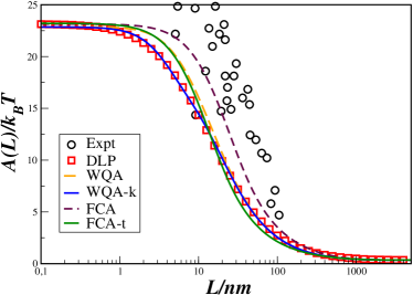
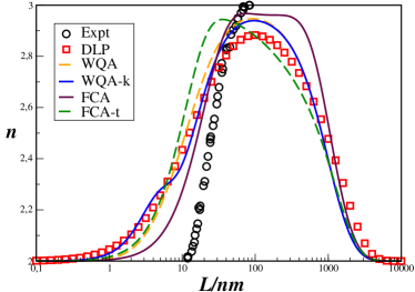
Figure 1: Hamaker function (left) and van der Waals effective exponent (right) for two mica plates interacting across vacuum at T=300 K. Circles are experimental results from Ref.Israelachvili and Tabor (1972). Squares are exact results from first order DLP theory Eq. (1). Lines are different approximations as described in the figure legend.

Unfortunately, even with $\nu_{\infty}$ assumed constant, the WQ approximation may be somewhat too cumbersome for some practical applications. Fortunately, we can obtain a simpler expression for $A_{\omega>0}(L)$ by taking into account that $\tilde{R}(x^{*},\nu)$ is expected to be a monotonically decaying function in most cases (an interesting exception is the system made of ice/water/air). Accordingly, applying the second mean value theorem of definite integrals to Eq. (6), one can write:

$$A_{\omega>0}(L)=\frac{3}{2}\frac{k_{B}T}{\nu_{T}}\tilde{R}(x^{*},\nu_{T})\int_{\nu_{T}}^{\nu_{\infty}}(1+\nu L)e^{-\nu L}d\nu$$ (16)

The above result is an exact quadrature for Eq. (6), provided one chooses a suitable $L$ dependent high frequency cutoff for the wave-number, $\nu_{\infty}$. This frequency acts effectively as a natural ultra-violet cutoff for the integral.

Performing now a trivial integration yields:

$$A_{\omega>0}=\frac{3\hbar c}{8\pi L}\tilde{R}^{*}_{\xi=0}\left[(2+\frac{3}{2}\nu_{T}L)e^{-\nu_{T}L}-(2+\nu_{\infty}L)e^{-\nu_{\infty}L}\right]$$ (17)

where the factor $3/2$ inside the first round parenthesis follows by inclusion of Euler-McLaurin corrections to lowest order. This accounts for the transformation of the sum Eq. (4) into an integral.

For practical matters, assuming a constant value for $\nu_{\infty}$ is sufficient. Indeed, by matching $\nu_{\infty}$ such that $A_{\omega>0}(L)$ yields the exact quadrature of Eq. (6) for $L=0$, we find:

$$\nu_{\infty}=t\,\frac{n_{m}\overline{n}_{1m}\overline{n}_{2m}}{\overline{n}_{1m}+\overline{n}_{2m}}\frac{\omega_{e}}{c}$$ (18)

where $\overline{n}_{im}=(n_{i}^{2}+n_{m}^{2})^{1/2}$ are root mean square indexes of refraction and $t=\pi/\sqrt{2}$ is a numerical factor (supporting information). We call this the Frequency Cutoff approximation (FCA).

The model is less accurate than the WQ approximation, but yields a qualitatively good agreement in the full range of relevant distances by using exactly the same parameters that are required to describe the Hamaker constant in usual applications.Israelachvili (1991) This contrasts with the few empirical approximations that have been previously suggested, which only provide heuristic estimates of the first crossover length-scale and completely neglect the second one.Sabisky and Anderson (1973); Gregory (1981); Cheng and Cole (1988) For ultimate simplicity, we can use Eq. (17) with the smooth function $\tilde{R}_{\xi=0}$ replaced by a constant $\tilde{R}_{\xi=0}(L=0)/t$, and choose $t=4$ to improve the decay rate of $A_{\omega>0}$ (supplemental material). In this way, the full Hamaker function may be readily given as:

$$\begin{array}[]{ccc}A_{\omega>0}(L)&=&\displaystyle{\frac{3\hbar c}{32\sqrt{2}\,n_{m}L}\left(\frac{n_{1}^{2}-n_{m}^{2}}{n_{1}^{2}+n_{m}^{2}}\frac{n_{2}^{2}-n_{m}^{2}}{n_{2}^{2}+n_{m}^{2}}\right)}\times\\ &&\\ &&\left[(2+\frac{3}{2}\nu_{T}L)e^{-\nu_{T}L}-(2+\nu_{\infty}L)e^{-\nu_{\infty}L}\right]\end{array}$$ (19)

Comparison of this very simple procedure (FC-t approximation) yields again an overall very good description of the full Hamaker function, at the cost of somewhat deteriorating the large $L$ behavior. We stress however, that the factor $t=4$ is model independent, so that this approach can now be applied generally for whatever system with overall very good accuracy. This is illustrated for interactions between two mica plates across water and for that of octane adsorbed on water (Fig.2), with dielectric relaxation parameters taken from Israelachvili.Israelachvili (1991) Particularly, our approach is able to capture the sign reversal of the Hamaker function for the water/octane/air system, where a description based on the Hamaker constant alone would be unable to predict the stabilization of thick octane films at the air/water interface.

As a caveat, notice that in either the WQ and FC approximations, the tractability of this approach relies on a one to one mapping of the effective cutoff frequency, $\nu_{\infty}$ with the resonance frequency $\omega_{e}$ of Eq. (15). Whence, the method is somewhat limitted to this simple optical description. For a more general sum of states, either Eq. (8) or Eq. (17) will still provide a correct qualitative description by mapping $\nu_{\infty}$ to the highest energy oscillator, provided the optical response function $R(x,n)$ decays monotonously.

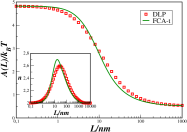
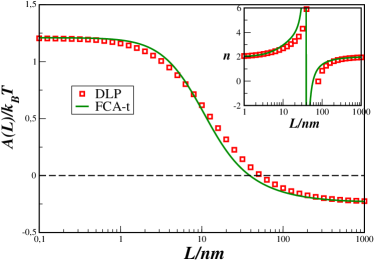
Figure 2: Comparison of Hamaker functions as obtained from DLP theory at T=300 K (symbols) with results from the FCA-t approximation (lines). Inset shows the effective van der Waals exponent. Left: mica/water/mica. Right: water/octane/air (notice the sign reversal of the Hamaker constant for this system).

Aside the quantitative description discussed above for selected systems, our approach illustrates qualitatively a number of very relevant issues that despite efforts (c.f. Parsegian (2006); French et al. (2010)) are generally not recognized. Firstly, the crossover from retarded to non-retarded interactions sets in for distances of the order $c/\omega_{e}$. For a large number of materials, including inorganic substrates and hydrocarbons, this corresponds to distances of about 10 nm,Chan and Richmond (1977); Hough and White (1980); Israelachvili and Adams (1978); Israelachvili (1991); Parsegian (2006); Boström et al. (2012) an order of magnitude less than it is often assumed.Gregory (1981) Secondly, the rather simple crossover function $A\approx A(0)(1+\nu_{\infty}L)^{-1}$ that is most often used in the literature yields a Hamaker constant that decays as $L^{-1}$ for large distances.Gregory (1981) In practice, the length scales $\nu_{\infty}$ and $\nu_{T}$ are not sufficiently well separated at ambient temperature, and the decay of the van der Waals interactions does never really attain the $L^{-3}$ power law expected from the Gregory equation. This can be illustrated by representing the effective exponent $n=d\ln g/d\ln L$.Israelachvili and Tabor (1972); Chan and Richmond (1977) Clearly, a regime of $n=3$ constant never really sets in at ambient temperature (Fig.1) Rather, $n$ reaches a maximum value that is close, but smaller than the ideal value of $3$ expected from the standard retardation regime. This observation is not specific to a particular choice of systems (Fig.2). It is dictated by the separation between the two constants $\nu_{\infty}$ and $\nu_{T}$, which is just two orders of magnitude at ambient temperature for most substances. In fact, using the FC approximation, it is possible to show that the Hamaker function decreases to half the Hamaker constant at distances $L_{1/2}=4\nu_{\infty}^{-1}$, whence, only a few times larger than the onset of retardation. Using this estimate for $L_{1/2}$ in either Eq. (8) or in Eq. (17) shows the Hamaker function obeys a scaling form $A_{\omega>0}(L)=A_{\omega>0}(0)u(L/L_{1/2})$, with $u(x)$ a universal function, as observed empirically by Cheng and Cole.Cheng and Cole (1988) As a final comment, we remark that the Gaussian Quadrature, which is a well known tool for numerical integration, can be exploited as an exceptional theoretical method in physics provided one chooses suitable problem adapted weight functions.

In summary, it was shown that a simple analytical crossover functions, Eq. (19) can be used to describe the Hamaker function in the range from the angstrom to the micrometer using exactly the same few material parameters that are employed conventionally to calculate the Hamaker constant. It is hoped this will allow for a much better quantification of intermolecular forces in a wide range of applications at the nanometric scale.Werner et al. (1999); Pototsky et al. (2005); French et al. (2010); Sánchez-Iglesias et al. (2012); Murata et al. (2016)

I Supplementary Material

See supplementary material for a detailed explanation of problem adapted one point Gauss quadrature rules, detailed derivation of Eq. (1), Eq. (4) Eq. (8), Eq. (17), calculation of the high-frequency cutoff, $\nu_{\infty}$ and parameters for the model systems.

Supporting Information for

Surface Van der Waals Forces in a Nutshell
by
Luis G. MacDowell

Departamento de Química Física, Facultad de Ciencias Químicas, Universidad Complutense, Madrid, 28040, Spain.

This document contains supporting information on the derivation of results from the main paper. To facilitate cross referencing, this materials is written as an appendix section. The equation numbering and bibliography follow the original paper, with equation labels and references not in this document referring to those of the original paper.

Appendix A DLP theory for the Hamaker constant

The exact result for the Hamaker function from DLP theory is:

$$A(L)=-\frac{3}{2}k_{B}T\sum_{n=0}^{\infty}\,{}^{\prime}\int_{r_{n}}^{\infty}x\ln([1-R^{M}_{1m2}(x,n)e^{-x}][1-R^{E}_{1m2}(x,n)e^{-x}])dx$$ (20)

with $R^{M}_{1m2}(x,n)=\Delta^{M}_{1m}(x,n)\Delta^{M}_{2m}(x,n)$, $R^{E}_{1m2}(x,n)=\Delta^{E}_{1m}(x,n)\Delta^{E}_{2m}(x,n)$, and

$$\begin{array}[]{lcl}\Delta^{M}_{ij}=\frac{x_{i}\epsilon_{j}-x_{j}\epsilon_{i}}{x_{i}\epsilon_{j}+x_{j}\epsilon_{i}}&&\Delta^{E}_{ij}=\frac{x_{i}\mu_{j}-x_{j}\mu_{i}}{x_{i}\mu_{j}+x_{j}\mu_{i}}\end{array}$$ (21)

while

$$x_{i}^{2}=x^{2}+(\epsilon_{i}\mu_{i}-\epsilon_{m}\mu_{m})(2\omega_{n}L/c)^{2}$$ (22)

where $\mu_{i}$ are magnetic permitivities and the rest of the notation as described in the main text.

In practice, all analytical approximations assume $R^{M}_{1m2}$ and $R^{E}_{1m2}$ are sufficiently smaller than unity that the logarithms can be Taylor expanded to first order. Furthermore, without any significant loss in accuracy one can also assume that the magnetic permitivities amount to unity in all three media. With these approximations, the above result becomes the first order approximation of Eq. (1). In our practice, this approximation is extremely accurate except for $L\to 0$, where next to leading terms in the expansion of the logarithm become relevant and can account for an additioan 5% contribution to the Hamaker constant.

Appendix B The Gaussian quadrature method

An n-point Gaussian quadrature rule is a numerical method where one seeks an approximation for the integral:

$$I=\int_{a}^{b}f(x)g(x)dx$$ (23)

such that

$$I\approx\sum_{i}^{n}f(x_{i})m_{i}$$ (24)

The set of points $\{x_{i}\}$ and weights $\{m_{i}\}$ are selected such that the integrals

$$I_{i}=\int_{a}^{b}x^{i}g(x)dx$$ (25)

up to $i=2n-1$ are exact. This guarantees tha the n-point method is exact for all polynomial $f(x)$ of degree $2n-1$ or less.

Appendix C Problem adapted one point Gauss quadrature as an analytical tool

In his book on van der Waals forces, Parsegian (2006) describes numerical methods for the calculation of the Hamaker function and strongly advocates the use of the Gaussian quadrature, claiming that evaluation of the integrand with just a few points is often sufficient for an accurate calculation. In our paper we pushed this claim to the maximum, by developing problem adapted one point quadrature rules. We have found this provides an extremely powerful general mathematical method for analytical calculations.

Accordingly, we attempt to evaluate the integral Eq. (23) as:

$$I=f(x^{*})m$$ (26)

To implement the one-point quadrature rule we calculate:

$$I_{0}=\int_{a}^{b}g(x)dx$$ (27)

and

$$I_{1}=\int_{a}^{b}xg(x)dx$$ (28)

exactly for the weight function $g(x)$. Then, according to the quadrature rule Eq. (26),

$$\begin{array}[]{ccc}I_{0}&=&m\\ I_{1}&=&x^{*}m\end{array}$$ (29)

So that trivially it follows

$$\begin{array}[]{ccc}m&=&I_{0}\\ x^{*}&=&\frac{I_{1}}{I_{0}}\end{array}$$ (30)

We find that this is an extremely powerful analytical tool provided that the weight functions $g(x)$ and interval of integration are chosen consistent with the physics of the problem in hand. i.e., in such a way that 1) the integral of $g(x)$ converges in the interval $[a,b]$ and 2) that the remaing function $f(x)$ is only weakly dependent on $x$.

Appendix D Quadrature for Eq. (1)

In Eq. (1) we seek to solve the integral

$$I=\int_{r_{n}}^{\infty}R(x)xe^{-x}dx$$ (31)

with $R(x)$ a bounded and smooth function. The convergence of the integral is therefore dictated by the term $xe^{-x}$. Accordingly, we choose $f(x)=R(x)$ and the weight function $g(x)=xe^{-x}$. Applying the one point quadrature rule, Eq. (26) we find:

$$I\approx R(x^{*})m$$ (32)

For the special case $r_{n}=0$, this corresponds to a generalized Gauss-Laguerre one-point quadrature rule. However, using the correct limit of integration is essential to describe the correct behavior. Therefore, we develop the rule adapted to match the physics of the problem. Using Eq. (27) and the range of integration between $r_{n}$ and $\infty$, the required integrals are trivially calculated and yield:

$$I_{0}=(1+r_{n})e^{-r_{n}}$$ (33)

$$I_{1}=(2+2r_{n}+r_{n}^{2})e^{-r_{n}}$$ (34)

Using this results, together with Eq. (30), yields Eq.8 and Eq.9 of the paper.

Appendix E Quadrature for Eq. (7)

In Eq. (7) we seek to solve the integral

$$I=\int_{\nu_{T}}^{\infty}R(x)[1+Lx]e^{-Lx}dx$$ (35)

Here, the convergence is dictated by $[1+Lx]e^{-Lx}$ for large $L$, but it is dictated by $R(x)$ for $L\to 0$. Accordingly, the natural weighting function for arbitrary $L$ is the full integrand. The corresponding integral cannot be given in general form for arbitrary dielectric functions. However, noticing that $R(x)$ is a smoothly convergent function that falls off for $x$ larger than a material parameter $\nu_{\infty}$, we write:

$$I=\int_{\nu_{T}}^{\infty}R(x)e^{x/\nu_{\infty}}\left[e^{-x/\nu_{\infty}}[1+Lx]e^{-Lx}\right]dx$$ (36)

With this device, the term in square brackets converges for arbitrary $L$, and is dominated by the $[1+Lx]e^{-Lx}$ for large $L$ as in the original integrand.

We can now apply the one-point quadrature rule Eq. (26) for the choice $f(x)=R(x)e^{x/\nu_{\infty}}$ and the weight function $g(x)=e^{-x/\nu_{\infty}}[1+Lx]e^{-Lx}$, so that:

$$I\approx R(x^{*})e^{x^{*}/\nu_{\infty}}m$$ (37)

For the special case $\nu_{T}=0$, the resulting quadrature corresponds to the sum of two generalized Gauss-Laguerre quadrature rules. Again, considering the lower integration limit is essential to retain the physics, so we develop a generalized Gauss-Laguerre quadrature with finite lower bound using Eq. (27). The required integrals are trivially calculated and yield:

$$I_{0}=\frac{1}{\nu_{\infty}}\frac{(\nu_{T}L+1)(\nu_{\infty}L+1)+\nu_{\infty}h}{(\nu_{\infty}L+1)^{2}}e^{-\nu_{T}L-\frac{\nu_{T}}{\nu_{\infty}}}$$ (38)

$$I_{1}=\frac{1}{\nu_{\infty}}\frac{(\nu_{T}L+1)(\nu_{\infty}L+1)^{2}\nu_{T}+(2\nu_{T}L+1)(\nu_{\infty}L+1)\nu_{\infty}+2\nu_{\infty}^{2}h}{(\nu_{\infty}L+1)^{3}}e^{-\nu_{T}L-\frac{\nu_{T}}{\nu_{\infty}}}$$ (39)

Using these results together with Eq. (30) yield Eq. (8) and Eq. (9) of the paper.

Appendix F Application of the Euler-McLaurin formula

The Euler-McLaurin formula allows to relate sums to integrals in exact form, and thus provides an estimate of the error that results from approximating a sum by an integral, as in the transformation from Eq. (4) to Eq. (6).

The formula states:

$$\sum_{n=a}^{b}f(n)=\int_{a}^{b}f(n)\,dn+\frac{1}{2}(f(a)+f(b))+\sum_{k=1}^{\infty}\frac{B_{2k}}{2k!}(f^{(2k-1)}(b)-f^{(2k-1)}(a))$$ (40)

where $B_{i}$ are the Bernoulli coefficients, and $f^{(m)}$ stands for $f$’s m-th derivative. Applying this formula to order $k=1$ to the sum of Eq. (4) we can obtain next to leading corrections, $\Delta A$, to the integral Eq. (6), with:

$$\Delta A=\frac{3}{2}k_{B}T\left[\frac{1}{2}R(x^{*},\nu_{T})(1+\nu_{T}L)e^{-\nu_{T}L}-\frac{1}{12}R(x^{*},\nu_{T})(\nu_{T}L)^{2}e^{-\nu_{T}L}\right]$$ (41)

where we have assumed that $\epsilon_{m}$ is constant for the infrared frequency $\omega_{T}$, such that $j_{m}=1$.

In the limit $L\to 0$, the correction to the Hamaker constant is of order $k_{B}T$, which is a small fraction of the exact result of order $\hbar\omega_{e}$. Only for $L\nu_{T}\gg 1$ does the corrections become of the same order as the integral. However, in that limit, the result obtained by integration changes only by a multiplicative factor of order unity. i.e., the qualitative behavior sought here remains unchanged.

The Euler-McLaurin corrections are particularly convenient in the framework of the FC approximation, since the corrections can be taken into account explicitely without any significant increasee in algebraic complexity. Indeed, integration of Eq. (16) yields:

$$A_{\omega>0}(L)=\frac{3\hbar c}{8\pi L}\tilde{R}^{*}_{\xi=0}[(2+\nu_{T}L)e^{-\nu_{T}L}-(2+\nu_{\infty}L)e^{-\nu_{\infty}L}]$$ (42)

While adding the correction $\Delta A$ to this expression now provides:

$$A_{\omega>0}=\frac{3\hbar c}{8\pi L}\tilde{R}^{*}_{\xi=0}[(2+\frac{3}{2}\nu_{T}L+\frac{1}{2}(\nu_{T}L)^{2}-\frac{1}{12}(\nu_{T}L)^{3})e^{-\nu_{T}L}-(2+\nu_{\infty}L)e^{-\nu_{\infty}L}]$$ (43)

whence, retaining only the zeroth order correction yields an improved expression whith exactly the same algebraic complexity as Eq. (42).

Appendix G Asymptotic expansion of $A_{\omega>0}$(L) for $L\to 0$.

In this section we show that the exact expansion of the Hamaker function for small $L$ features next to leading order terms exhibiting the logarithmic singularity of $O(L^{2}\ln L)$.

To show this we first notice the small $L$ expansion of $\Delta_{im}$ corresponds to an expansion in powers of $r_{n}$ about $r_{n}=0$. Accordingly, we find:

$$\Delta_{im}=\frac{\epsilon_{i}-\epsilon_{m}}{\epsilon_{i}+\epsilon_{m}}+\frac{(\epsilon_{i}-\epsilon_{m})\epsilon_{i}}{(\epsilon_{i}+\epsilon_{m})^{2}}\frac{r_{n}^{2}}{x^{2}}$$ (44)

Notice the variable $x$ appears as $x^{-2}$ in the second order term of the expansion. Upon integration, this will result in the logarithmic singularity mentioned before. Using the above result for $\Delta_{im}$, we can now write:

$$R_{1m2}^{M}(x,n)=R_{0}+R_{2}\frac{r_{n}^{2}}{x^{2}}$$ (45)

with

$$R_{0}=\frac{\epsilon_{1}-\epsilon_{m}}{\epsilon_{1}+\epsilon_{m}}\frac{\epsilon_{2}-\epsilon_{m}}{\epsilon_{2}+\epsilon_{m}}$$ (46)

and

$$R_{2}=\frac{(\epsilon_{1}-\epsilon_{m})(\epsilon_{2}-\epsilon_{m})\epsilon_{2}}{(\epsilon_{1}+\epsilon_{m})(\epsilon_{2}-\epsilon_{m})^{2}}+\frac{(\epsilon_{1}-\epsilon_{m})(\epsilon_{2}-\epsilon_{m})\epsilon_{1}}{(\epsilon_{2}+\epsilon_{m})(\epsilon_{1}-\epsilon_{m})^{2}}$$ (47)

Performing the integration over $x$, we find:

$$\int_{r_{n}}^{\infty}R_{1m2}^{M}(x,n)xe^{-x}dx=R_{0}[1+r_{n}]e^{-r_{n}}+R_{2}r_{n}^{2}Ei(r_{n})$$ (48)

where $Ei(x)$ is the exponential integral. We find that right beyond the zero order contribution, the problem becomes plagued with the non-elementary exponential integral. Expanding this result for small $L$, we obtain the lowest order correction to the Hamaker function as:

$$A_{\omega>0}(L)=A_{\omega>0}(0)-\frac{3}{2}k_{B}T\sum_{n=1}^{\infty}\left\{\frac{1}{2}R_{0}+[\gamma+\ln(\nu_{n}L)]R_{2}\right\}(\nu_{n}L)^{2}$$ (49)

where $\nu$ is defined here as in the paper and $\gamma$ is the Euler constant. Notice that this small $L$ expansion does not bare any contribution from $R_{1m2}^{E}(x,n)$, which only provides terms of order $L^{4}$ or higher.

Appendix H Second mean value theorem of definite integrals

According to the second mean value theorem, if $f(x)$ is a monotonic function and $g(x)$ is an integrable function in the interval $(a,b)$, there exists a constant $a<c<b$, such that:

$$\int_{a}^{b}f(x)g(x)dx=f(a^{+})\int_{a}^{c}g(x)dx+f(b^{-})\int_{c}^{b}g(x)dx$$ (50)

This statement is also true when $b\to\infty$, provided that $f(x)$ and $g(x)$ are bounded functions in the interval $(a,\infty)$.

In order to apply the theorem to solve Eq. (6), we consider $x=\nu$, $a=\nu_{T}$, $b=\infty$, $f(\nu)=\tilde{R}(x^{*},\nu)$ and $g(\nu)=(1+\nu L)e^{-\nu L}$. Then, we find:

$$A_{\omega>0}(L)=\frac{3\hbar c}{8\pi}\tilde{R}(x^{*},\nu_{T})\int_{\nu_{T}}^{\nu_{\infty}}(1+\nu L)e^{-\nu L}d\nu$$ (51)

This theorem is physically appealing as it implies the existence of a natural ultraviolet cutoff for the improper integral of Eq. (6). Performing the remaining trivial integration yields the result of Eq. (17).

Appendix I Calculation of the high frequency cutoff

The high frequency cutoff, $\nu_{\infty}$ is calculated by matching the approximate expression for $A_{\omega>0}$ in the limit of $L\to 0$, with the exact result in that limit.

In the WQ approximation, taking Eq. (8) in the limit of $L\to 0$ one finds:

$$A_{\omega>0}^{WQ}(L\to 0)=\frac{3}{2}k_{B}T\frac{\nu_{\infty}\epsilon_{m}^{1/2}(i\nu_{T})}{\nu_{T}\epsilon_{m}^{1/2}(i\nu_{\infty})}j_{m}^{-1}(\nu_{\infty})R(2,\nu_{\infty})\,e$$ (52)

where we have taken into account that $x^{*}=2$ for $L=0$, and we have assumed $\nu^{*}=\nu_{T}+\nu_{\infty}\approx\nu_{\infty}$. By matching this result with the exact Hamaker constant, a trascendental equation for $\nu_{\infty}$ is obtained. In practice, it is far more convenient to rewrite the wave numbers in terms of angular frequencies (i.e., $\nu_{k}=2\epsilon^{1/2}(i\nu_{k})\omega_{k}/c$). Taking this into account, the result simplifies to:

$$A_{\omega>0}^{WQ}(L\to 0)=\frac{3\hbar\omega_{\infty}}{4\pi}j_{m}^{-1}(\omega_{\infty})R(2,\omega_{\infty})\,e$$ (53)

matching this result with the exact Hamaker constant provides a trascendental equation for $\omega_{\infty}$.

In the FC approximation, one obtains:

$$A^{FC}_{\omega>0}(L\to 0)=\frac{3}{2}k_{B}T\frac{\nu_{\infty}}{\nu_{T}}j_{m}^{-1}(\nu_{T})R(2,\nu_{T})$$ (54)

where again we took into account that $x^{*}=2$. Matching the above result with the exact Hamaker constant, a simple linear equation for $\nu_{\infty}$ is obtained.

More explicit results may be obtained for specific choices of the dielectric functions.

I.1 Specific results for the damped oscillator model

In the damped oscillator model, the dielectric function is given as:

$$\epsilon(i\omega)=1+\frac{n^{2}-1}{1+(\omega/\omega_{e})^{2}}$$ (55)

I.1.1 Hamaker constant

The exact Hamaker constant in the linear approximation of Eq. (1), is given as:

$$A_{\omega>0}(L=0)=\frac{3}{2}k_{B}T\sum_{n=1}^{\infty}\left(\frac{\epsilon_{1}-\epsilon_{m}}{\epsilon_{1}+\epsilon_{m}}\right)\left(\frac{\epsilon_{2}-\epsilon_{m}}{\epsilon_{2}+\epsilon_{m}}\right)$$ (56)

where we have taken into account that in this limit ($L\to 0$), $R_{1m2}^{E}$ vanishes exactly, while $R_{1m2}^{M}$ becomes independent of $x$, so that the integration over $x$ may be performed trivially. Conventionally, in this approximation the sum is now replaced by an integral, while the three materials are assumed to have the same characteristic high energy absorbtion frequency $\omega_{e}$. A second integration over the fequencies then provides the known result:

$$A_{\omega>0}(L=0)=\frac{3\hbar\omega_{e}}{8\sqrt{2}}\frac{(n_{1}^{2}-n_{m}^{2})(n_{2}^{2}-n_{m}^{2})}{(n_{1}^{2}+n_{m}^{2})^{1/2}(n_{2}^{2}+n_{m}^{2})^{1/2}[(n_{1}^{2}+n_{m}^{2})^{1/2}+(n_{2}^{2}+n_{m}^{2})^{1/2}]}$$ (57)

We use below this result as the ’exact’ Hamaker constant.

I.1.2 WQ approximation

In the WQ approximation, the damped oscillator model for the dielectric functions yields:

$$R(2,\omega_{\infty})=\left(\frac{\omega_{e}^{2}(n_{1}^{2}-n_{m}^{2})}{\omega_{e}^{2}(n_{1}^{2}+n_{m}^{2})+2\omega_{\infty}^{2}}\right)\left(\frac{\omega_{e}^{2}(n_{2}^{2}-n_{m}^{2})}{\omega_{e}^{2}(n_{2}^{2}+n_{m}^{2})+2\omega_{\infty}^{2}}\right)$$ (58)

Replacing this result into Eq. (52), matching the resultant approximate Hamaker constant with that of Eq. (57) and introducing the factor $f$ such that $\omega_{\infty}=f(n_{1}+n_{m}^{2})^{1/4}(n_{2}^{2}+n_{m}^{2})^{1/4}\omega_{e}$, we obtain:

$$\left(1+\frac{1}{2}\frac{d\ln\epsilon_{m}}{d\ln\omega}\right)^{-1}\frac{e\,q^{2}f}{(1+2q^{2}f^{2})(q^{2}+2f^{2})}=\frac{\pi}{2\sqrt{2}}\frac{q}{q^{2}+1}$$ (59)

where $q=(n_{1}^{2}+n_{m}^{2})^{1/4}/(n_{2}^{2}+n_{m}^{2})^{1/4}$. This is a complicated trascendental equation for $f$, but simplifies very much when the interactions between material 1 and 2 take place across vacuum, such that $\epsilon_{m}$ is a constant. For the additional simplification that materials 1 and 2 are the same, $q=1$, one obtains $f=0.5934$

I.1.3 FC approximation

In the FC approximation, the damped oscillator model for the dielectric functions yields:

$$R(2,\omega_{T})=\left(\frac{n_{1}^{2}-n_{m}^{2}}{n_{1}^{2}+n_{m}^{2}}\right)\left(\frac{n_{2}^{2}-n_{m}^{2}}{n_{2}^{2}+n_{m}^{2}}\right)$$ (60)

where we have assumed that $\omega_{T}/\omega_{e}\ll 1$. Replacing this result into Eq. (54) and matching the resulting approximate Hamaker constant with that of Eq. (57), yields:

$$\nu_{\infty}=f(n_{1}^{2}+n_{m}^{2})^{1/4}(n_{2}^{2}+n_{m}^{2})^{1/4}n_{m}\frac{\omega_{e}}{c}$$ (61)

with

$$f=\frac{\pi}{\sqrt{2}}\frac{q}{q^{2}+1}$$ (62)

where we have taken into accout that for a single oscillator in the UV region, $j_{m}=1$ at the thermal frequency $\omega_{T}$. Alternatively, the above result can be given explictely in terms of the refraction indexes as:

$$\nu_{\infty}=\frac{\pi}{\sqrt{2}}n_{m}\frac{(n_{1}^{2}+n_{m}^{2})^{1/2}(n_{2}^{2}+n_{m}^{2})^{1/2}}{(n_{1}^{2}+n_{m}^{2})^{1/2}+(n_{2}^{2}+n_{m}^{2})^{1/2}}\frac{\omega_{e}}{c}$$ (63)

Appendix J Working formulae in the FCA-t approximation

For ease of implementation we provide here the final working formula in the FCA-t approximation:

$$A_{\omega>0}(L)=\frac{3\pi k_{B}T}{8\sqrt{2}\nu_{T}L}\left(\frac{n_{1}^{2}-n_{m}^{2}}{n_{1}^{2}+n_{m}^{2}}\frac{n_{2}^{2}-n_{m}^{2}}{n_{2}^{2}+n_{m}^{2}}\right)\left[(2+\frac{3}{2}\nu_{T}L)e^{-\nu_{T}L}-(2+\nu_{\infty}L)e^{-\nu_{\infty}L}\right]$$ (64)

or

$$A_{\omega>0}(L)=\frac{3\hbar c}{32\sqrt{2}\,n_{m}L}\left(\frac{n_{1}^{2}-n_{m}^{2}}{n_{1}^{2}+n_{m}^{2}}\frac{n_{2}^{2}-n_{m}^{2}}{n_{2}^{2}+n_{m}^{2}}\right)\left[(2+\frac{3}{2}\nu_{T}L)e^{-\nu_{T}L}-(2+\nu_{\infty}L)e^{-\nu_{\infty}L}\right]$$ (65)

where the wave-numbers $\nu_{T}$ and $\nu_{\infty}$ are:

$$\left\{\begin{array}[]{ccc}\nu_{T}&=&\frac{4\pi k_{B}Tn_{m}}{c\hbar}\\ &&\\ \nu_{\infty}&=&4n_{m}\frac{(n_{1}^{2}+n_{m}^{2})^{1/2}(n_{2}^{2}+n_{m}^{2})^{1/2}}{(n_{1}^{2}+n_{m}^{2})^{1/2}+(n_{2}^{2}+n_{m}^{2})^{1/2}}\frac{\omega_{e}}{c}\end{array}\right.$$ (66)

Appendix K Material parameters for the oscillator model

K.1 mica/air/mica

For the interaction of two mica plates across air we used data for muscovite mica described using the dielectric response given by Eq. (15), with parameters obtained from high frequency data by Bergström (1997), i.e., $n^{2}=2.508$ and $\omega_{e}=1.963\cdot 10^{-16}$ rad/s. The static permitivity is $\epsilon(0)=5.4$.

K.2 mica/water/mica

For the interaction of mica across air we employ the one oscillator model with data as summarized in Israelachvili (1991). Parameters for water are $\epsilon(0)=80$, $n^{2}=1.7769$ and $\omega_{e}=1.885\cdot 10^{-16}$ rad/s. Parameters for mica are $\epsilon(0)=7.0$, $n^{2}=2.56$ and $\omega_{e}=1.885\cdot 10^{-16}$ rad/s.

K.3 octane/water/air

For the interaction of a water film adsorbed on the octane/air interface we use parameters for water as described above, and the parameters for octane as given in Israelachvili (1991), i.e., $\epsilon(0)=1.95$, $n^{2}=1.9238$ and $\omega_{e}=1.885\cdot 10^{-16}$.