Learning from Higher-Layer Feature Visualizations

Abstract

Driven by the goal to enable sleep apnea monitoring and machine learning-based detection at home with small mobile devices, we investigate whether interpretation-based indirect knowledge transfer can be used to create classifiers with acceptable performance. Interpretation-based indirect knowledge transfer means that a classifier (student) learns from a synthetic dataset based on the knowledge representation from an already trained Deep Network (teacher). We use activation maximization to generate visualizations and create a synthetic dataset to train the student classifier. This approach has the advantage that student classifiers can be trained without access to the original training data. With experiments we investigate the feasibility of interpretation-based indirect knowledge transfer and its limitations. The student achieves an accuracy of 97.8% on MNIST (teacher accuracy: 99.3%) with a similar smaller architecture to that of the teacher. The student classifier achieves an accuracy of 86.1% and 89.5% for a subset of the Apnea-ECG dataset (teacher: 89.5% and 91.1%, respectively).

1 Introduction

In our project we aim to enable Obstructive Sleep Apnea (OSA) monitoring and detection at home with consumer electronics. Machine learning has shown to be rather efficient for OSA detection, e.g., [24]. To be able to run classifiers on mobile computing devices with restricted resources, e.g., smart phone or smart watch, we need to develop an approach to create small classifiers with high performance.

Literature suggests that larger deeper neural networks outperform smaller shallower ones on large, challenging datasets [9, 10, 6]. This insight triggered the idea to leverage the knowledge representation of deep neural networks (DNN) to train the small classifier, i.e., to use knowledge transfer to improve its performance. There exist many knowledge transfer techniques (see Section 2). However, the challenge we address is different from existing approaches, because we want to transfer knowledge from a larger classifier (teacher) to a smaller classifier (student) and we want to do this independently of learning method and without access to the original training data. The latter is due to the many issues with sharing health data of patients (in our case sleep monitoring data).

The essence of the knowledge transfer approach presented in this paper is to re-use recent visualization-based results for interpretable machine learning with a new goal. Instead of using visualizations to enable a human expert to understand the internals of a model, we use the visualization approach to create a synthetic dataset to train the student classifier. Therefore, we call this approach interpretation-based indirect knowledge transfer. We take advantage of the fact that neuronal activation is generally multi-faceted [18] to create a synthetic dataset of visualization with the diversity that has the capability to train a student classifier. Our experimental work reveals that our goal that a student classifier trained on the synthetic dataset achieves better performance than if it would have trained on the original training set cannot be met. However, we show that the larger the synthetic dataset is, the better the performance of the student classifier such that it is possible to come close to this goal using the proposed technique.

We analyze the impact of the architectural similarity of student and teacher and investigate the performance of interpretation-based knowledge transfer between different learning methods, i.e., from a Convolutional Neural Network (CNN) to Support Vector Machines (SVM), Random Forest (RF), and a Multilayer Perception architecture (MLP). Our results show that the more similar student and teacher are architecturally and algorithmically, the higher the performance of the student trained on the visualizations.

We introduce two new metrics to measure the difficulty that other trained classifiers have in identifying the synthesized data, and whether we can pass ”hidden” messages from a classifier to another without the other classifiers (the majority of them) realizing it. Based on these metrics, we evaluate the performance of the synthesized dataset in comparison to the real dataset. The other trained classifiers are either CNN or humans.

Our Contributions: (1) We demonstrate that a classifier can learn from the feature visualizations of another classifier. (2) We develop a novel technique of knowledge transfer that does not require the training data for the student to train and is independent of architecture or algorithm for the student network. It makes the student generalize with various degrees of success to the real data depending on the architectural or algorithmical proximity between student and teacher and the generating algorithm. (3) Two new metrics that give quantitative measures for difficulty in interpreting the visualizations applicable to any point in the feature space.

The remainder of this paper is structured as follows. In Section 2 we present a more detailed analysis of related work. In Section 3 we explain the design of our method and we evaluate the proposed technique in Section 4. In Section 5 we present conclusions and future work.

2 Related Work

Recently, many new techniques for transfering knowledge have been proposed, especially with the goal to reduce the size of a DNN to decrease the execution time and reduce memory consumption. Existing model compression techniques, e.g., via pruning or parameter sharing [4, 8, 7, 23] can be considered as a form of knowledge transfer from a trained teacher to a student. Other types of methods, transfer the knowledge from a smaller to a larger DNN to make it learn faster [3] or even between different task domains [19, 25].

In the knowledge distillation method [14], the student network is trained to match the softmax output layer logits of the trained teacher network and the classes of the original data. [22] introduce fitnets, an extension of the knowledge distillation method to train thinner deeper networks (student) from wider shallower ones (teacher). [2] investigate the compression of large ensembles (like RF, bagged decision trees, etc.) via the use of a very small artificial neural network (ANN). As a universal approximator the ANN is able to generalize to mimic the learned function of the ensemble given sufficient data. To train the ANN they create a larger synthetic dataset based on the real dataset that is labeled by the ensemble. [14] use knowledge distillation on a selection of informative neurons of top hidden layers to train the student network. The selection is done by minimizing an energy function that penalizes high correlation and low discriminativeness.

It is worth noting that our technique differs from the above since we do not aim to perform any form of knowledge distillation. Our aim is for the student to independently train on a synthetic dataset created by capturing learned high-layer features of the teacher. For this reason, the original data is not needed to train the student. Our technique is additionally applicable to different learning algorithms.

Regarding the understanding of internal representations of a DNN, [5] introduce the activation maximization (AM) technique, among others, for qualitative evaluation of higher-level representations of the internal representations of two unsupervised deep architectures. [17] generate fooling images either directly or indirectly (via a compositional pattern producing network) encoded via maximizing the output layer of a DNN. They show that the images produced can be unrecognizable for a human observer. In their follow up work, [16] use a deep generative network to synthesize images that maximize the output of a neuron of a certain layer of the network. We base our approach on some of these insights.

3 Method

In this section, we explain intepretation-based indirect knowledge transfer from a more general perspective, present our proposed architecture, and specify the procedure we use to generate the synthetic dataset.

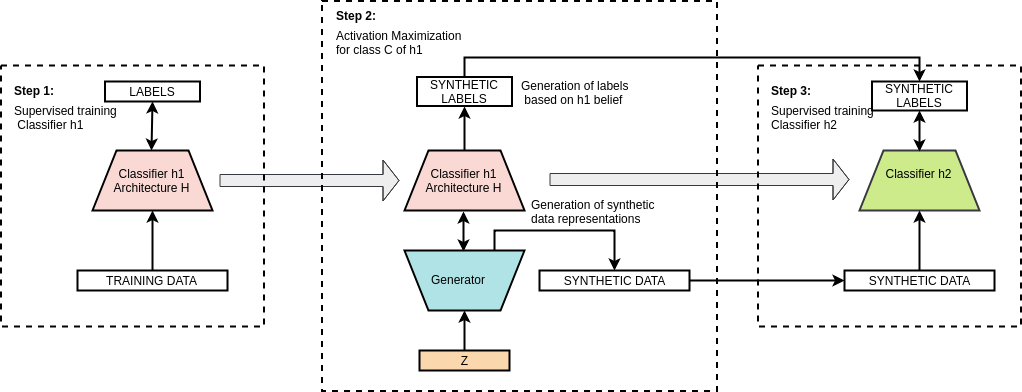
Figure 1: The Generating procedure we follow includes AM via using a generator network G similarly to [16].

3.1 Intepretation-Based Indirect Knowledge Transfer

We are interested in transferring the knowledge of a given trained DNN $h_{1}$ to another model or learning algorithm $h_{2}$. We assume that the original data with which $h_{1}$ is trained is not available for training $h_{2}$. We aim to enable $h_{2}$ to classify data that come from the same distribution as $D$ with a similar performance as $h_{1}$. The only way to achieve this without access to $D$ is to extract the knowledge accumulated by $h_{1}$. We perform this by generating visualizations that correspond to strong beliefs of what $h_{1}$ assumes a class is. These visualizations will then be used as a synthetic dataset to train $h_{2}$.

We define intepretation-based indirect knowledge transfer for a classifier $h_{2}$ to mean the following: a model $h_{1}$ is first trained on $D$ with distribution $p_{Data}$. Then a generation procedure $Gen\{h_{1}\}$ produces a dataset $D_{2}$ to train classifier $h_{2}$.

Depending on the success of $Gen\{h_{1}\}$ to map the important features from the task domain learned by $h_{1}$ into $D_{2}$, and the algorithmic and architectural similarity between $h_{1}$ and $h_{2}$, we show that it is possible for $h_{2}$ to learn to perform the classification task $h_{1}$ has learned.

3.2 Design

Our proposed design (see Figure 1) is based on three basic steps:

Step 1 - Training of the teacher. We train the teacher network $h_{1}$ in a supervised manner with $D$ to learn the underlying data distribution $p_{Data}$. This requires the original labeled training data.

Step 2 - Creating the synthetic dataset. To enable indirect knowledge transfer, we create a synthetic dataset $D_{2}$ that captures features that $h_{1}$ has learned from training on $D$. $Gen\{h_{1}\}$ is used to create this synthetic dataset, and is one of the core elements of the method. In $Gen\{h_{1}\}$, we perform AM via a deep generator network (G) that transforms a small noise vector Z to examples that strongly activate a predefined neuron (see Section 3.3 for further details). Inspirations for this design were [1, 16]. After the synthetic set is created we create its labels. If $\mathbf{x_{s}}$ corresponds to a synthetic example created by $Gen\{h_{1}\}$, we give $\mathbf{x_{s}}$ the label that $h_{1}$ chooses for it, i.e., either the class with the maximum output probability, $\arg\max_{i}\{h_{1_{iL}}(\theta,\mathbf{x_{s}})\}$ where $i$ corresponds to the possible class of the output, L denotes the output layer of $h_{1}$ and $\theta$ corresponds to the parameter vector of $h_{1}$, or the softmax of the output to better capture the output probabilities of $h_{1}$.

Step 3 - Training of the student. As final step the student $h_{2}$ is trained via the synthetic data and labels produced by step 2. $h_{2}$ can be smaller or larger DNN than the $h_{1}$, or even be based on a different learning method.

The choice of $Gen\{h_{1}\}$ and which method to use for $h_{2}$ are two central decisions. Next, we discuss the choice of $Gen\{h_{1}\}$ and in Section 4 we evaluate the performance of different $h_{2}$ methods.

3.3 Generation

For knowledge extraction and generation we consider two visualization approaches: AM and code inversion [15]. However, code inversion requires the original training data, or the logits of the data from the fully connected layer we will try to match. This defeats our goal to train $h_{2}$ without access to $D$. Therefore, we use AM for the generation of the synthetic dataset. Contrary to other works like [16] the goal of $Gen\{h_{1}\}$ is not to produce realistic looking synthetic data, but instead to investigate whether we can reliably train $h_{2}$ from the synthetic dataset and how sensitive the procedure is to the choice of the architecture or learning method of $h_{2}$.

To synthesize data that the trained model $h_{1}(\theta,x)$ perceives as of class $i$, $Gen\{h_{1}\}$ uses AM [5] on the activations of output layer L of $h_{1}(\theta,x)$ via G such that:

$$\theta^{*}_{G}=\arg\max_{\theta_{G}s.t||G(\theta_{G},\mathbf{Z})||\leq R}\{h_{1_{iL}}(\theta,G(\theta_{G},\mathbf{Z}))\}$$ (1)

where $i$ corresponds to the class we want to find a visualization for. $\theta$ is the parameter vector of $h_{1}$, and $\theta_{G}$ the parameter vector of G. Note that $\theta$ is static because $h_{1}$ is already trained and we are optimizing for $\theta_{G}$ given varying ”pseudo inputs” of $\mathbf{Z}$. $R$ is the maximum value of the norm of the output of G for a given norm (we use sigmoids on the output of G), and $L$ denotes the output layer. We choose to perform AM in the output layer of $h_{1}$ since we want visualizations that correspond to a strong belief for a class in $h_{1}$. We use $\mathbf{Z}$ as an input random noise vector (mainly from a uniform distribution) which G transforms into the visualization. We intentionally do not give any additional priors to $Gen\{h_{1}\}$, since we do not want to constrain our exploration of the movement in the feature space.

We stop the AM when the output of the target class neuron $i$ is higher than all the other ouput neurons and exceeds a threshold T:

$$h_{1_{iL}}(\theta,G(Z,\theta_{G}^{*}))>T$$ (2)

This implies that the space that satisfies Eq.(2) is a subspace of the space of class $i$, as defined by its decision boundaries. We assume that softmax activation is used on the output layer.

We specify the the loss of G to maximize the logits of each class of the classifier ($h_{1}$ in Figure 1). We then repeat the procedure for a number of iterations, and end up with a synthetic dataset comprised of the visualizations of $h_{1}$ for all of the classes.

3.3.1 Reinitializations

The goal of $Gen\{h_{1}\}$ is to generate visualizations such that $h_{2}$ can learn and generalize to D. We therefore need to generate many visualizations of each class. However, with the procedure above we get data from the same limited neighborhood of the feature space, depending on the variation of the input noise Z in G. To ensure that we capture the space of a class defined by $h_{1}$ better, we reinitialize $\theta_{G}$ and repeat the procedure a certain number of times until there is no additional improvement on the generalization capability of $h_{2}$. We test this by measuring $h_{2}$ accuracy on the test data. We find that repeated initializations of $\theta_{G}$ with the default truncated normal initializer almost always yield the same class for $h_{1}$. A test with 1000 reinitializations of $\theta_{G}$ resulted in, $argmax_{c}\{h_{1}(\theta,G(\theta_{G},z))\}$ always having the same class. This indicates that the initial subspace covered by the output of G is constrained to a subspace of the space of this class.

Due to the small default weight initializations in relation to the total space, the potential starting points for the output of G are generally confined. Additionally, AM is hindered when we increase the initial weights to relatively large values (by varying the truncated initializer). This might be attributed to very large values for the generated images (output of G) that are very close to 0 or 1 which have a negative effect to the learning procedure. This problem is also related to the variance or limits of $\mathbf{Z}$. However, we cannot increase this variance without limit, as this also hinders learning (a higher variance implies inconsistently large numbers, which leads to stronger activations). In summary, potentially we cannot capture all of the important parts of $p_{Data}$ that $h_{1}$ has learned due to limitations in the randomness of the initial $\theta_{G}$ and $\mathbf{Z}$, depending on the loss landscape. We therefore perform an initial step of pseudorandom movement in the feature space (i.e., output space of G and input of $h_{1}$) before the actual AM.

3.3.2 Attraction-Repulsion for diversity

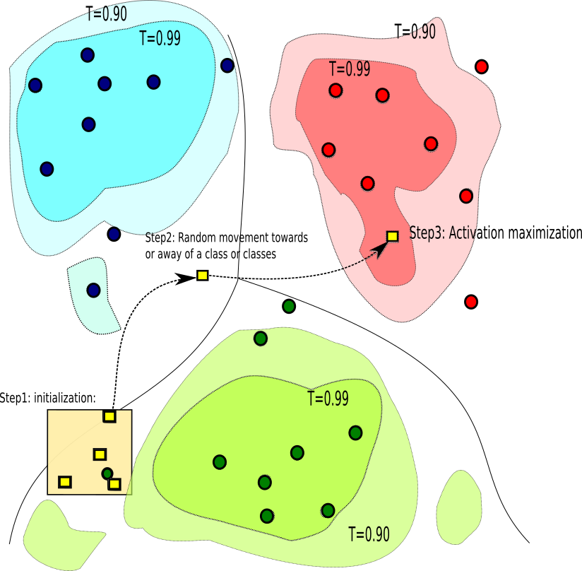
Figure 2: Example of the generation procedure.

We perform pseudorandom movements via optimizing $\theta_{G}$ to either maximize or minimize the $h_{1}$ activation for a random subset of classes. This is performed across a random number of steps. This pre-AM step changes the initial position of the output of G in the feature space as defined by $\theta_{G}$. If the change in the initial position is sufficient, the entering to the subspace which satisfies our AM threshold from Eq.(2) can potentially capture a different facet of the strong output neuronal activation. In Figure 2 we show an example. The green, red, and blue dots depict data points. The green, red, and blue areas depict areas of the feature space that satisfy Eq.(2) for the maximum logit class neuron of $h_{1}$. The lighter regions depict areas where threshold T is smaller and thus are supersets of the previous. The yellow rectangles depict points of G with different parameter tunings during Steps 1-3. In Step 1 after the initialization the position is defined from the randomized vector $\theta_{G}$ and from $\mathbf{Z}$. Since both are confined, the output of G will also be confined ($l_{\infty}$ hypershere). In Step 2 we execute the pseudorandom movement. In Step 3 AM towards the specified class (red) is performed.

4 Evaluation

In this section, we investigate the viability of the proposed approach. We perform three experiments. Experiment 1 (Section 4.1) acts as an empirical proof of concept. We examine the performance of different student $h_{2}$ architectures and methods on the MNIST dataset [12]. As $h_{1}$ we use a small CNN and as G a small deconvolutional deep generator. Since we are interested in studying the impact of different architectures and learning methods we do not use existing pre-trained classifiers, e.g., LeNet [12].

We study in Experiment 1 a modification of the proposed method: we specify the additional goal on G, to maximize the $l_{2}$ distance from the real data (for this experiment we access the original data) in the second to last hidden layer of $h_{1}$, to instigate visualizations with high level features that are not in D. We investigate whether we can learn with this added constraint.

The last part of Experiment 1 serves as a basis for Experiment 2 (Section 4.2). In Experiment 2 we examine the ability of a set S of potential learning methods to predict $h_{1}$ beliefs for a given set of visualizations. Based on this, we define properties to measure the absolute and relative difficulty of the set S in performing this task. We also evaluate this on the basis of each classifier of S independently.

In Experiments 1 and 2, we demonstrate that: (1) $h_{2}$ can learn from the visualizations albeit to varying degrees of success depending on the learning method and (2) that the visualizations are interpetable using a third method (or set of methods) to varying degrees of success depending on the architectural and algorithmic similarity with $h_{1}$. In Experiment 3, we use a realistic healthcare application to evaluate both aspects of our approach simultaneously (Section 4.3).

4.1 Proof of Concept with MNIST Dataset

For $h_{1}$ we use a small CNN with dropout (conv-maxpool-conv-maxpool-fc1-dropout-fc2-sigmoid). We use seven different $h_{2}$: (1) A CNN that has exactly the same architecture as $h_{1}$ (CNN_ID). (2) A network that has similar architecture as $h_{1}$, but is smaller with half of the channels for all the convolutional layers and half of the neurons in the fully connected layers (CNN_S). (3) A network that is larger than $h_{1}$, with one convolutional and one fully connected layer more, and that has different pooling and activation functions, i.e., average instead of max for pooling and elu instead of relu for activations (CNN_L ). (4) A convolutional network with even less weights than CNN_S (CNN_s). (5) A MLP architecture with a small perceptron with three hidden layers and relu activations. (6) A simple SVM. (7) A RF with 100 trees.

We test these classifiers as $h_{2}$ on the test set of the MNIST dataset. Table 1 presents the classification results for the baseline (when $h_{2}$ is trained with the real data) and the synthetic dataset. Additionally, we experiment with soft labels and randomized constrained T. Our best results are: an accuracy of 98.13$\pm$0.03% for CNN_ID and 97.84$\pm$0.06% for CNN_S (see Appendix).

Table 1: Results for 60000 visualizations. T=0.99, hard labels

$h_{2}$ Acc(%)	Base	$h_{1}$Vis.
CNNID	99.30$\pm$0.03	95.51$\pm$0.28
MLP	94.80$\pm$0.10	48.91$\pm$0.18
RF	92.12$\pm$0.10	23.20$\pm$1.40
SVM	94.04$\pm$0.00	39.71$\pm$0.00
CNNS	99.23$\pm$0.03	95.11$\pm$0.33
CNNL	99.42$\pm$0.03	94.53$\pm$0.41
CNNs	98.89$\pm$0.03	91.80$\pm$0.30

The results in Table 1 show a clear trend that when $h_{2}$ has the same or similar CNN architecture like $h_{1}$, it is able to learn from the synthetic visualizations and generalize relatively efficiently to the real test data. However, we observe a significantly lower performance for the other classifiers, i.e., MLP, RF, and SVM. Since all clasifiers are able to succesfully learn the visualization classes during training the lower performance is caused by a lower generalization capability. However, most of the algorithms are generalizing better than random choice.

For simpler algorithms like SVMs we can give a potential explanation for the low performance. As shown in Figure 2 and in [17], inside the class boundaries of a trained model (in our case $h_{1}$), exist regions of high confidence that are sparse in the sense that they do not contain many data points from the training data. Since we try to capture these high confidence regions from different directions (via the randomized repeated initializations), there can be cases where (1) areas that are not in the original data distribution are captured and (2) areas that are in the data distribution, are not captured sufficiently by the synthetic dataset. For the SVM, the final decision hyperplane after the training on the vizualizations can be very different from the original, because it works with points that are near the boundaries (the support vectors), and these boundary data points can be very different in the synthetic dataset due to the aforementioned reasons.

Images from this procedure for MNIST can be found in the Appendix. In the following sections we investigate how $h_{2}$ performance changes as we increase the number of visualizations synthesized.

4.1.1 Size of the synthetic dataset

We evaluate the performance of $h_{2}$ with increasing size of the synthetic dataset. As reference, we measure the performance of $h_{2}$ with subsets of the original training data with the same size as the synthetic dataset. $h_{2}$ has exactly the same architecture as $h_{1}$ in this experiment.

Table 2: Accuracy vs size of the synthetic dataset.

Data size(#)	Acc Synth	Acc Real
400	63.0$\pm$2.0	92.5$\pm$0.2
2000	85.5$\pm$1.1	96.8$\pm$0.1
4000	87.5$\pm$1.1	98.3$\pm$0.02
12000	92.7$\pm$ 0.5	98.8$\pm$0.02
20000	94.0$\pm$0.1	99.1$\pm$0.05
40000	94.8$\pm$0.2	99.3 $\pm$0.01
60000	95.5$\pm$0.3	99.3$\pm$0.02
80000	95.7$\pm$0.2	-

Table 2 shows that increasing the size of the synthetic dataset has a positive effect on the performance of $h_{2}$. As expected, training with visualizations is much less efficient than training with the real data. For any given accuracy, we need more synthetic data than original data. On the other hand, the synthetic dataset can be arbitrarily large, which means that the performance of $h_{2}$, as long as $h_{2}$ has the capacity, could match that of $h_{1}$. This also depends on $Gen\{h_{1}\}$, learning the important features learned from $h_{1}$.

4.1.2 Avoiding High Level Features of D

We evaluate how well $h_{2}$ can train with visualizations that are intentionally dissimilar from the real data in terms of the features captured by high-layer neurons that are not output neurons. Inspired by [21] and [13], and knowing that higher-layer neurons map predominantly high-level semantics [5], for a given distance metric, we maximize the distance between the logits for real and generated data for an intermediate fully connected layer:

$$Loss_{2}=-\sum_{n=0}^{B_{s}}d(h_{1_{L-1}}(\theta,\mathbf{x}_{n}),h_{1_{L-1}}(\theta,G(\theta_{G},\mathbf{z})))$$ (3)

where all $\mathbf{x}_{n}\in D_{i}$ where $D_{i}$ is the subset of $D$ with labels of class $i$ assuming that we perform AM for class $i$. For simplicity we choose $l_{2}$ as distance metric $d$. $B_{s}$ is the size of the batch and $L-1$ denotes the second to last layer. Therefore, we want to capture features that activate maximally the output (class) neuron, but are far from the ones of the real data in the previous layer. During training of G we perform this update (i.e., movement) and AM in separate steps, and we use a learning rate that is $1/3-1/5$ of that of the learning rate of AM depending on the pseudorandom movement (see Section 3.3 ).

After the synthesis of the visualizations with the extra condition, we train a $h_{2}$ with the same architecture as $h_{1}$ but with different weight initializations. We get an accuracy of 94.33$\pm$0.12 for a synthetic dataset with 60000 images, while the original procedure achieves 95.51% accuracy.

4.2 Difficulty of Interpretation

Next, we investigate how difficult it is for classifiers with different architectures to find the class which an example $\mathbf{x}_{s}$ (visualization for our experiments) is classified by $h_{1}$. To measure the total difficulty of a set S of different methods, we define two properties: the fooling example and hidden message. We use these properties to evaluate how difficult it is for different sets of classifiers to identify visualizations produced using the CIFAR10 dataset.

4.2.1 Property Definitions

We define two properties of points in the feature space to quantify how difficult if is for a set of classifiers $S$ to identify the decision of $h_{1}$ for a given example $\mathbf{x_{s}}$. The fooling example property provides a direct estimate, whereas the hidden message property provides a relative estimate in relation to another student network $h_{2}$.

In the following definitions, let $S=\{h_{1},h_{2}...h_{N}\}$ with $h_{i}\in H$, $h_{i}:X\rightarrow Y,i=1...N$, where H is the space of possible classifiers and $|S|=N$. For a given metric $m(h_{j},D)\in[0,1]$ , a dataset $D_{T}=\{(\mathbf{x}_{1},\mathbf{y}_{1}),(\mathbf{x}_{2},\mathbf{y}_{2}),...,(\mathbf{x}_{M},\mathbf{y}_{M})\}$ with $\mathbf{x}_{1},...\mathbf{x}_{N},\in X$ and a given threshold $A\in[0,1]$ ,we have that $m(h_{i},D_{T})>A$ $\forall$ $h_{i}\in S$ (assuming higher m means better performance). First, we redefine the fooling examples from [17] using the notion of a comparative set S:

Definition 4.1.

Fooling example: Given classifier $h\notin S$, we define a fooling example for S to be a $\mathbf{x}_{s}\in X$ such that, $h(\mathbf{x}_{s})=l\in Y$, and there exist a subset of S such that $S_{c}=\{h_{i}\in S|h_{i}(\mathbf{x})=c\neq l,c\in Y$ } with $|S_{c}|>N/2$.

Thus, if the majority of S disagrees with $h$ on the class of $\mathbf{x}_{s}$ we have a fooling example for S. $h_{1}...h_{N}$ may be humans. Since the given A is non-negative we want all of our classifiers to be able to perform the classifications of $\mathbf{x}$ and the test set $D_{T}$. The classifiers should also be able to perform acceptably for the given metric, i.e., the metric m should be above a certain given threshold A for the test set $D_{T}$ and classifier $h_{i}$, $i=1...N$.

Notice that the dimensionality of the feature space can be different between different classifiers as long as the classifier is capable of classifying for different dimensions. The more data with the fooling example property we have for a given dataset $D_{s}$, the more difficulty S has in identifying decisions from $h$ for this dataset.

Definition 4.2.

Hidden message: Given two classifiers $h$,$h_{s}\notin S$, we define a hidden message for S to be an example $\mathbf{x}_{s}\in X$ such that $h(\mathbf{x}_{s})=h_{s}(\mathbf{x}_{s})=l\in Y$, and there exist a subset of S such that $S_{h}=\{h_{i}\in S|h_{i}(\mathbf{x}_{s})=c\neq l,c\in Y$ } with $|S_{h}|>N/2$.

The hidden message property implies that $h$ and $h_{s}$ agree on the class decision for the example $\mathbf{x}_{s}$ while the majority of S disagrees. For a given dataset $D_{s}$, this property measures the difficulty that S has to identify data points where $h$ and $h_{s}$ agree on, or from the perspective of $h$ and $h_{s}$ how easy it is for S not to notice examples of agreement. $h$ can be thought as having the role of teacher for the context of intepretation-based indirect knowledge transfer.

4.2.2 Quantification of Difficulty

We use the CIFAR10 dataset [11] to evaluate different student classifiers, as it is easily recognizable by humans, but not as easy as MNIST. We exclude the non-deep learning methods from the previous experiment due to their inferior performance.

We use a CNN as $h_{1}$ which achieves an accuracy of 86.72% on the test set. $h_{1}$ is used as ”Teacher” ($h$ in the property definitions) for two sets of classifiers $S_{1}$ and $S_{2}$. $S_{1}$ comprises two CNNs: CNN2 which has a larger architecture (more layers, more activations) and CNN3 which has a larger architecture, and with different activations (see Appendix for details). For $S_{2}$ we use an enseble of five humans. We train the classifiers with the original training data, and give the humans a sample to get experience with the images.

The accuracies for the test set are in the first column of Table 3 and 4. Additionally, a CNN with exactly the same architecture to $h_{1}$ (called CNN1) will be used as $h_{s}$ for both $S_{1}$ and $S_{2}$. With AM we produce 100 images (10 for each class) that have $h_{1}$ logits of at least 99% for the target class (denoted as IMGS). We calculate the percentage of images that a classifier agrees on the decision of the class with $h_{1}$ on. Following the procedure from Section 4.1.2, we synthesize 100 more images (denoted as IMGS+L).

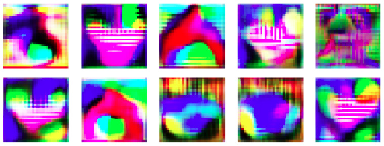
Figure 3: Visualizations from the AM on CIFAR10 .

We calculate the percentage of the dataset which satisfies the fooling example and hidden message properties. For $S_{1}$ we use the entire test set of CIFAR10 for this. Since humans would be overwhelmed to classify the entire CIFAR10 test set, we use 100 random subsamples from the test set for $S_{2}$. The synthetic datasets also include only 100 images each, in order to be feasible for human classification.

Table 3: Results for $S_{1}$

	CIFAR10 Acc(%)	imgs(%)	imgs+L(%)
CNN1($h_{s}$)	88.6	89.0	75.0
CNN2($\in S_{1}$)	90.65	75.0	51.0
CNN3($\in S_{1}$)	88.25	69.0	67.0
Hidden M.($S_{1}$)	2.4	9.0	11.0
Fooling Ex.($S_{1}$)	8.4	11.0	21.0

Table 4: Results for $S_{2}$. Using 100 images

$h\in$S2	sample Acc(%)	imgs(%)	imgs+L(%)
subject1	86	26	12
subject2	93	40	29
subject3	84	16	18
subject4	89	20	27
subject5	91	39	24
Fooling Ex.($S_{2}$)	9	81	89
Hidden M.($S_{2}$)	5	74	67

We see the humans achieve a similar performance for the given sample as the CNNs (although the CNNs are evaluated with the whole dataset). Second, for IMGS and especially for IMGS$+$L, the performance drops for all members of $S_{1}$ and $S_{2}$. Additionally, the percentage of examples that satisfy both properties increases. This means that the identification of what $h_{1}$ believes as classes for the examples of the datasets becomes increasingly difficult to identify both for the individual members of the sets, and for the combined decision of the sets. A very interesting point is that the human ability to identify images in IMGS and IMGS$+$L is much lower than that of the members of $S_{1}$.

4.3 Case Study: Creating Non-identifiable Training Data from Apnea Recordings

Using ML techniques to automatically detect sleep apnea in arbitrary computer devices is hindered by the fact that sufficient trainining data is not available for many developers due to privacy and ownership issues. Therfore, we evaluate whether we can benefit from the difficulty of interpreting the visualizations. On a subset of an open access apnea dataset called Apnea ECG [20] we perform intepretation-based indirect knowledge transfer with $h_{1}$ and $h_{2}$ having the same architectures. We train one network to distinguish between periods of normal breathing and periods with sleep apnea, and another network to distinguish between two possible teams of people from which the sleep recordings are obtained. We examine the ability of student to learn from the visualizations, and the ability of the identifier network to distinguish between the two teams for the real and synthetic data. We use full overnight sleep recordings from eight patients. Every minute of the recording is labelled. We have two possible classes: an Obstructive Sleep Apnea (OSA) event happened or not.

Table 5: Apnea-ECG results

$h_{2}$ Acc(%)	Base OSA	$h_{2}$ S.	$h_{idt}$ R.	$h_{idt}$ S.
Team 1	92.49	89.5	91.07	56.36
Team 2	86.69	86.10	89.98	58.74

We separate these data into training, validation, and test sets via random subsampling and train a classifier $h_{1}$ to perform classification of OSA events per minute in the test set. Additionally, we train another classifier ($h_{idt}$) on the same training and test sets, but with the goal to identify the person from which the data was recorded. This means that $h_{idt}$ outputs one of eight possible classes regarding the eight patients. By using the procedure from Section 3.3, we generate a synthetic dataset, and we train a classifier $h_{2}$ with the same architecture as $h_{1}$. Finally, we evaluate whether $h_{idt}$ can identify the recordings for the synthetic dataset.

To perform the experiments we need to refine the generation process. For the real data, we know which person the data originated from. But for the generated data, we do not have access to the labels of the person which the generated example corresponds to. Thus, we cannot measure the performance of $h_{idt}$ on the synthetic data. To avoid this issue, we split the recordings into two teams of four people and follow the same procedure as before for each team separately. Then we train $h_{idt}$ to identify the team from which the data originates instead of the individual.

Table 5 presents our results. All the results regard the real test set. The second column (Base OSA) shows the results for a classifier trained on the real data on Team1 or Team 2 and tested on the real test set. The third column ($h_{2}$ S. ) denotes a classifier $h_{2}$ with identical architecture and activations to the original, trained with the examples of the learned features (the synthetic dataset) from the original for Team 1 or Team 2 which also performs classification on the test set. Columns 4 and 5 depict the accuracy of $h_{idt}$ in recognizing which team each example originates from for the real test data (Column 4) and for the synthetic data (Column 5).

There is a clear drop in the performance of $h_{idt}$ from the real to the synthetic data which means that $h_{idt}$ does not recognize as easily the team which the synthetic data was generated from as the team that data from the test set originate. Additionally the synthetic data can be used to train $h_{2}$ to achieve almost similar performance to $h_{1}$ (Base OSA) for both teams.

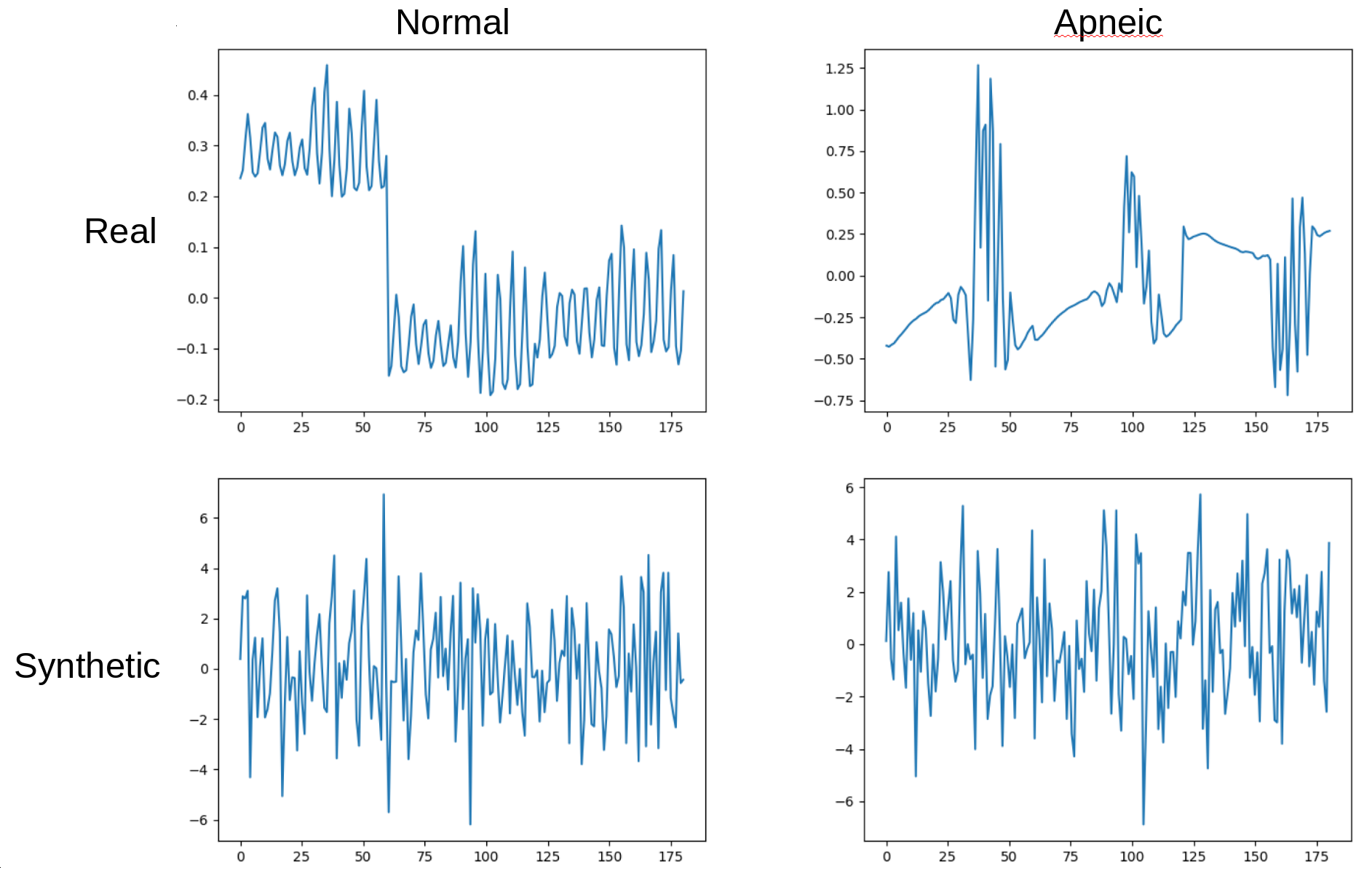
Figure 4: Example of real and generated Apnea-ECG data

5 Conclusions

In this paper we propose an approach for interpretation-based indirect knowledge transfer between two classifiers $h_{1}$ and $h_{2}$. Using AM on the output logits of $h_{1}$, G can interpret the knowledge that $h_{1}$ has about the distribution $p_{Data}$ of a dataset D, and generate visualizations of these interpretations. We then perform supervised learning of $h_{2}$ using only these visualizations. A primary benefit of this is that $h_{2}$ can learn an approximation of $p_{Data}$ without access to the original dataset D. Furthermore, since the interpretation of G is guided only by the output logits of $h_{1}$, the resulting visualizations primarily contain features that are important to identify the target class. An added benefit is therefore that other, potentially sensitive information in $D$ is neglected from the visualizations. To strengthen this aspect, we extend G with a loss function $Loss_{2}$ that explicitly penalizes visualizations that contain high-level features of $D$.

We evaluate our approach experimentally with both computational and human classifiers. When $h_{1}$ and $h_{2}$ have similar architectures and algorithms (e.g., CNN of similar size), $h_{2}$ can successfully be trained using only the visualizations (i.e., without D). We achieve an accuracy of up to 95.51% (for the same size of dataset as the real) on MNIST and 89.5% on Apnea-ECG. Interestingly, the accuracy drops gradually as the difference between $h_{1}$ and $h_{2}$ increases. This is particularly visible with human classifiers with a maximum accuracy of 40% and 29% with and without $Loss_{2}$, respectively. We develop new metrics to quantify this difficulty of learning, i.e., the fraction of points in the feature space that have one of two key properties: a fooling example is one that is mostly mis-classified by classifiers in a set S that differ from $h_{1}$, and a hidden message is one that is correctly classified by a classifier $h_{s}$ similar to $h_{1}$, and is elsewise mostly mis-classified by S. With visualizations obtained using the CIFAR10 dataset, and where classifiers in S and $h_{1}$ are CNN that differ in size, 11% and 18% of the visualizations are fooling examples, with and without $Loss_{2}$, respectively, and 9% and 14% are hidden messages. When S contains humans and $h_{s}$ is a CNN exactly the same in architecture to $h_{1}$, 81% and 89% are fooling examples and 74% and 67% are hidden messages. Our visualizations can be especially useful in a healthcare context where $D$ with sensitive information cannot be used directly. Using sleep recordings from the Apnea-ECG database, we demonstrate that: (1) our visualizations can be used to successfully train classifiers to detect sleep apnea, and (2) classifiers trained to identify groups of individuals in $D$ are incapable of discriminating between these groups in the visualizations.

As future work we plan to reduce the time it takes to synthesize visualizations and the number of examples necessary to achieve good performance. As a next step we aim to investigate whether we can leverage interpretation-based knowledge transfer to realize differetial privacy for sleep apnea data.

Appendix A Soft Labels and Randomized T

We evaluate the performance of CNN_ID for different sizes of the dataset. Here instead of giving a standard threshold T (as for example $T=0.99$), each time we perform activation maximization, we randomly choose a different value of T between 0.90 and 0.99. When we implement this change, we get the following results (Table 6):

Table 6: Results T=0.90-0.99, hard labels

Size (# of examples )	Acc CNNID (%)
60000 examples	95.74$\pm$0.15
120000 examples	96.47$\pm$0.03
180000 examples	96.65$\pm$0.17

and: a score of 96.17% for CNN_S for 180000 examples (visualizations). We additionally ran the other classifiers, but we did not observe big differences in their performance.

After that we additionally used soft labels for the CNN_ID and we got the following results:

Table 7: Results T=0.90-0.99, soft labels

Size (# of examples )	Acc CNNID (%)
400 examples	82.04$\pm$1.03
4000 examples	94.93$\pm$0.28
45000 examples	97.18$\pm$0.11
60000 examples	97.90$\pm$0.01
120000 examples	98.13$\pm$0.03

and for CNN_S we experimented with 120000 samples and got an accuracy of: 97.84$\pm$0.06.

Appendix B CIFAR10 synthetic test sets

IMGS and IMGS+L datasets (Figures 5, 6).

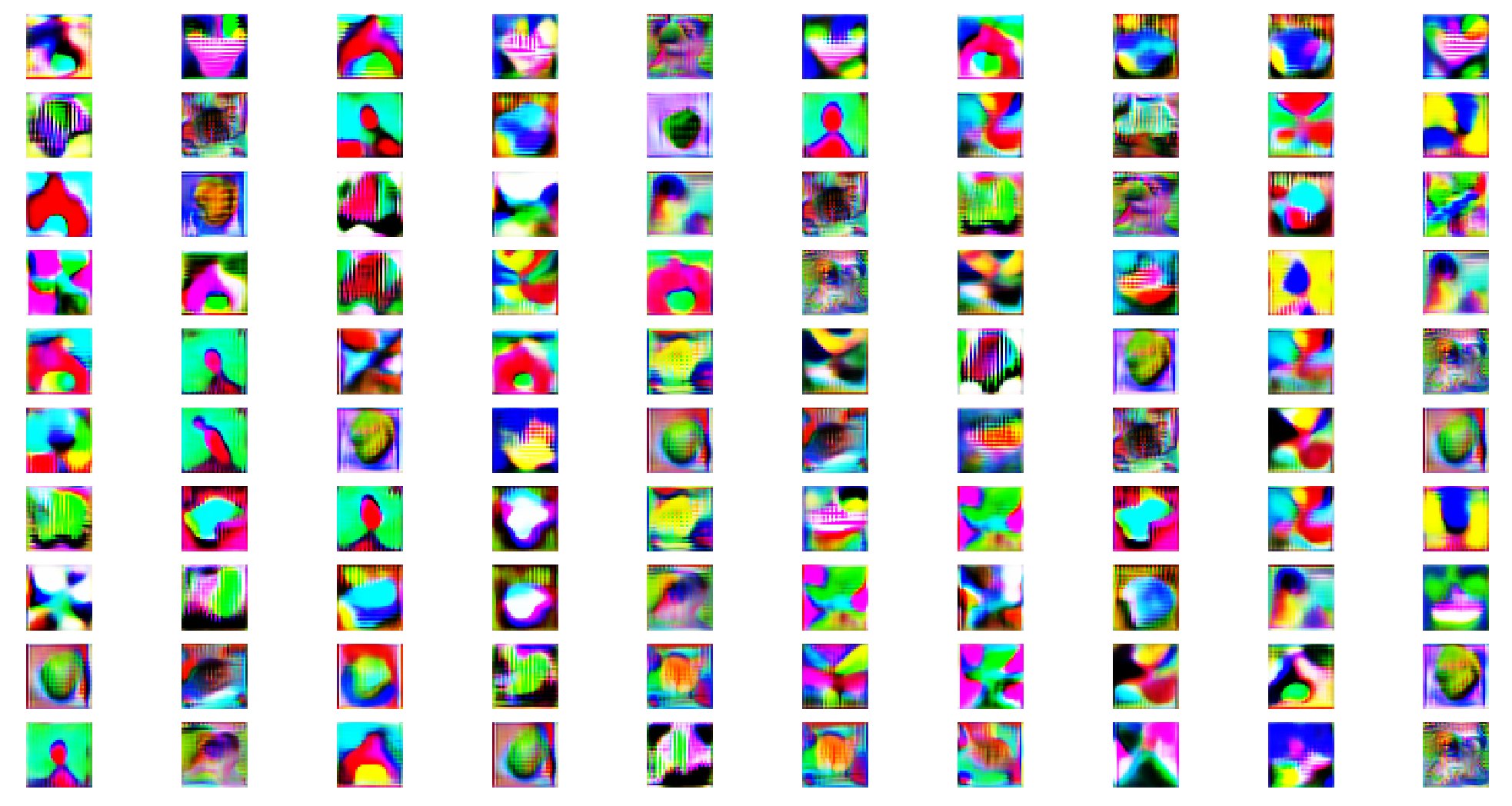
Figure 5: IMGS

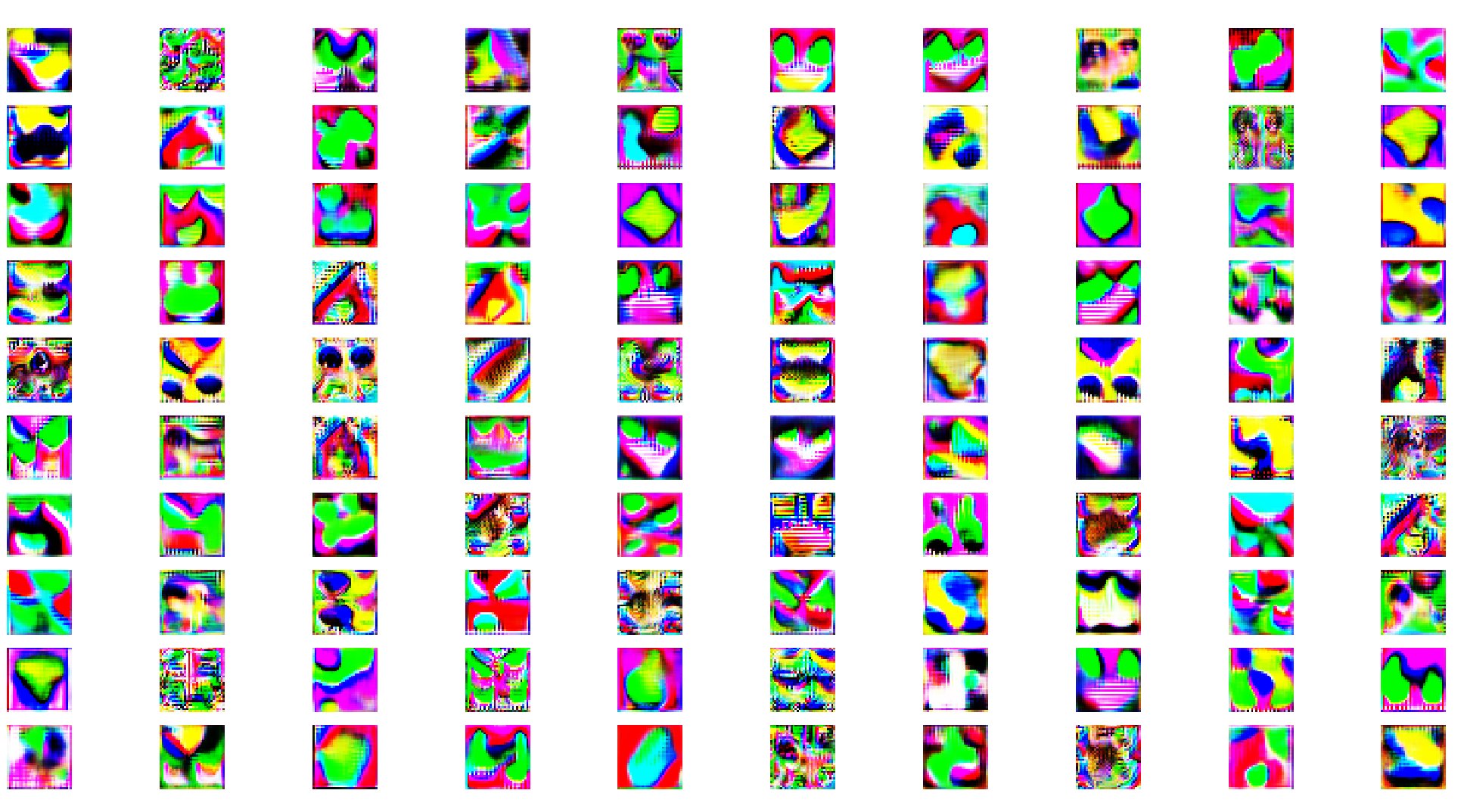
Figure 6: IMGS+L

Appendix C Examples of MNIST visualizations

Examples of visualizations of MNIST (Figures 7,8,9). Each batch (9 imgs) corresponds to different pre-AM movement (Batch 1. Attraction toward one random class. Batch 2. Repulsion from many classes Batch 3. Attraction to many classes). Notice that the movement is not the only difference between the Batches. Parameters like learning rate and minibatch size also change per Batch.

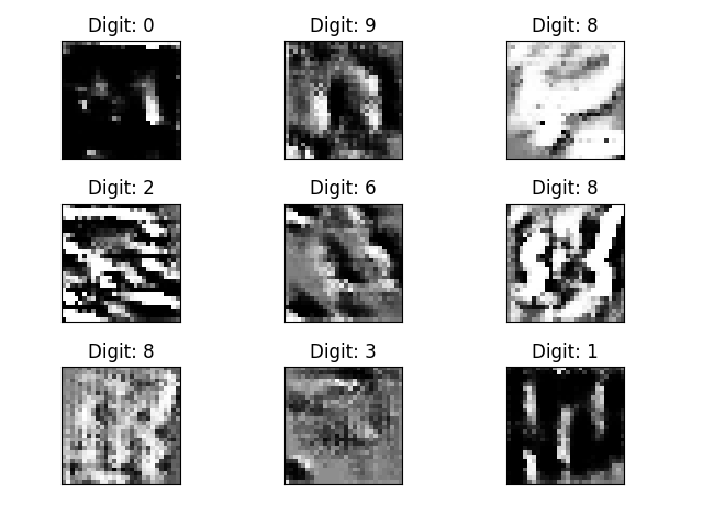
Figure 7: Batch1

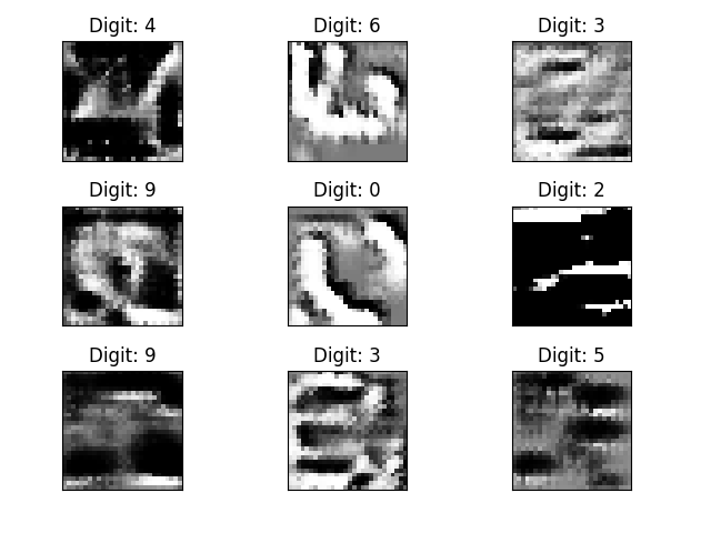
Figure 8: Batch2

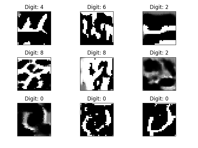
Figure 9: Batch3

Appendix D CIFAR10 Architectures of CNN1, CNN2 and CNN3

For Experiment 2 (the CIFAR10 experiments) we wanted CNN2 and CNN3 that form $S_{1}$ to be at least near equal in terms of performance on the original CIFAR10 test set to the performances of the CNN that acts as $h_{1}$ ( the ”Teacher”-or h for the hidden message/fooling example property-called CNN${}_{h_{1}}$) and of CNN1, which acts as $h_{s}$ from the hidden message property. That way we have a stronger means of quantification of the ”difficulty” of assumingly progressively harder to interpret datasets (from CIFAR10 test set to IMGS and then to IMGS+L) via using $S_{1}$. General Architectures:

• CNN1=CNN${}_{h_{1}}$: 6 convolutional 1 dense (elu activations) + batchnorm+dropout+data augmentation(ImagedataGenerator, rotation, horizontal flip width shift length shift)

• CNN2: 10 conv 1 dense (elu activations)+ batchnorm+dropout+data augmentation(ImagedataGenerator, rotation, horizontal flip width shift length shift)

• CNN3: 10 conv 3dense (relu activations)+ batchnorm+dropout+data (no augm)

References

- [1] Shumeet Baluja and Ian Fischer. Adversarial transformation networks: Learning to generate adversarial examples. arXiv preprint arXiv:1703.09387, 2017.
- [2] Cristian Buciluǎ, Rich Caruana, and Alexandru Niculescu-Mizil. Model compression. In Proceedings of the 12th ACM SIGKDD international conference on Knowledge discovery and data mining, pages 535–541. ACM, 2006.
- [3] Tianqi Chen, Ian Goodfellow, and Jonathon Shlens. Net2net: Accelerating learning via knowledge transfer. arXiv preprint arXiv:1511.05641, 2015.
- [4] Yu Cheng, Duo Wang, Pan Zhou, and Tao Zhang. A survey of model compression and acceleration for deep neural networks. arXiv preprint arXiv:1710.09282, 2017.
- [5] Dumitru Erhan, Yoshua Bengio, Aaron Courville, and Pascal Vincent. Visualizing higher-layer features of a deep network. University of Montreal, 1341(3):1, 2009.
- [6] Ian Goodfellow, Yoshua Bengio, Aaron Courville, and Yoshua Bengio. Deep learning, volume 1. MIT press Cambridge, 2016.
- [7] Song Han, Jeff Pool, John Tran, and William Dally. Learning both weights and connections for efficient neural network. In Advances in neural information processing systems, pages 1135–1143, 2015.
- [8] Babak Hassibi and David G Stork. Second order derivatives for network pruning: Optimal brain surgeon. In Advances in neural information processing systems, pages 164–171, 1993.
- [9] Kaiming He, Xiangyu Zhang, Shaoqing Ren, and Jian Sun. Deep residual learning for image recognition. In Proceedings of the IEEE conference on computer vision and pattern recognition, pages 770–778, 2016.
- [10] Andrew G Howard, Menglong Zhu, Bo Chen, Dmitry Kalenichenko, Weijun Wang, Tobias Weyand, Marco Andreetto, and Hartwig Adam. Mobilenets: Efficient convolutional neural networks for mobile vision applications. arXiv preprint arXiv:1704.04861, 2017.
- [11] Alex Krizhevsky, Vinod Nair, and Geoffrey Hinton. The cifar-10 dataset. online: http://www. cs. toronto. edu/kriz/cifar. html, 2014.
- [12] Yann LeCun, Léon Bottou, Yoshua Bengio, and Patrick Haffner. Gradient-based learning applied to document recognition. Proceedings of the IEEE, 86(11):2278–2324, 1998.
- [13] Ming-Yu Liu and Oncel Tuzel. Coupled generative adversarial networks. In Advances in neural information processing systems, pages 469–477, 2016.
- [14] Ping Luo, Zhenyao Zhu, Ziwei Liu, Xiaogang Wang, Xiaoou Tang, et al. Face model compression by distilling knowledge from neurons. In AAAI, pages 3560–3566, 2016.
- [15] Aravindh Mahendran and Andrea Vedaldi. Visualizing deep convolutional neural networks using natural pre-images. International Journal of Computer Vision, 120(3):233–255, 2016.
- [16] Anh Nguyen, Alexey Dosovitskiy, Jason Yosinski, Thomas Brox, and Jeff Clune. Synthesizing the preferred inputs for neurons in neural networks via deep generator networks. In Advances in Neural Information Processing Systems, pages 3387–3395, 2016.
- [17] Anh Nguyen, Jason Yosinski, and Jeff Clune. Deep neural networks are easily fooled: High confidence predictions for unrecognizable images. In Proceedings of the IEEE Conference on Computer Vision and Pattern Recognition, pages 427–436, 2015.
- [18] Anh Nguyen, Jason Yosinski, and Jeff Clune. Multifaceted feature visualization: Uncovering the different types of features learned by each neuron in deep neural networks. arXiv preprint arXiv:1602.03616, 2016.
- [19] Sinno Jialin Pan, Qiang Yang, et al. A survey on transfer learning. IEEE Transactions on knowledge and data engineering, 22(10):1345–1359, 2010.
- [20] Thomas Penzel, George B Moody, Roger G Mark, Ary L Goldberger, and J Hermann Peter. The apnea-ecg database. In Computers in cardiology 2000, pages 255–258. IEEE, 2000.
- [21] Konda Reddy Mopuri, Utkarsh Ojha, Utsav Garg, and R Venkatesh Babu. Nag: Network for adversary generation. In Proceedings of the IEEE Conference on Computer Vision and Pattern Recognition, pages 742–751, 2018.
- [22] Adriana Romero, Nicolas Ballas, Samira Ebrahimi Kahou, Antoine Chassang, Carlo Gatta, and Yoshua Bengio. Fitnets: Hints for thin deep nets. arXiv preprint arXiv:1412.6550, 2014.
- [23] Suraj Srinivas and R Venkatesh Babu. Data-free parameter pruning for deep neural networks. arXiv preprint arXiv:1507.06149, 2015.
- [24] MB Uddin, CM Chow, and SW Su. Classification methods to detect sleep apnea in adults based on respiratory and oximetry signals: a systematic review. Physiological measurement, 39(3):03TR01, 2018.
- [25] Junho Yim, Donggyu Joo, Jihoon Bae, and Junmo Kim. A gift from knowledge distillation: Fast optimization, network minimization and transfer learning. In 2017 IEEE Conference on Computer Vision and Pattern Recognition (CVPR), pages 7130–7138. IEEE, 2017.