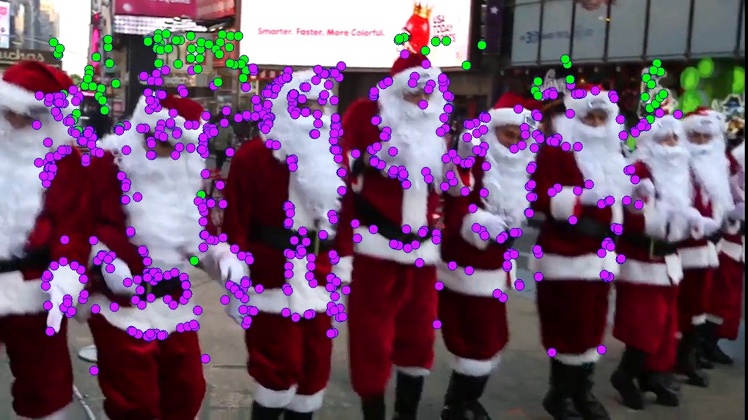
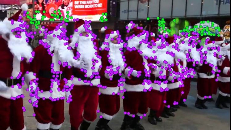
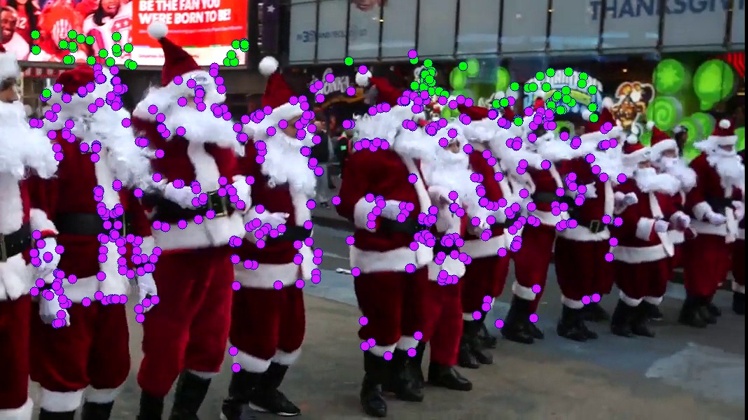
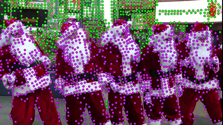
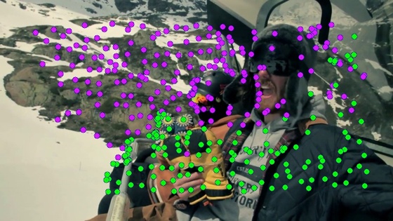
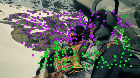
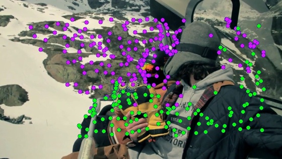
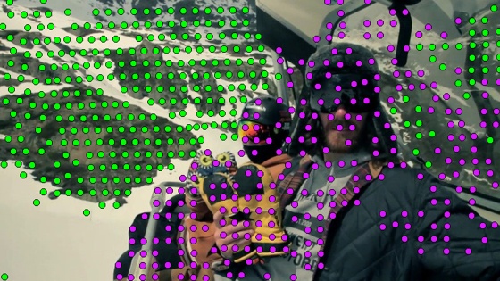
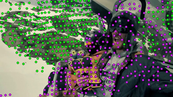
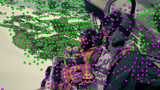
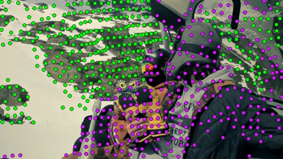
11email: linkaimo1990@gmail.com, {eleclf,elexuxu}@nus.edu.sg 22institutetext: Shenzhen Cloudream Technology, China
22email: {jiangnj,jiangbo}@cloudream.com
Robust Video Background Identification by Dominant Rigid Motion Estimation††thanks: This work was supported by the Singapore PSF grant 1521200082, and partly done when Kaimo, Nianjuan and Jiangbo were with Advanced Digital Sciences Center (ADSC), Singapore.
Abstract
The ability to identify the static background in videos captured by a moving camera is an important pre-requisite for many video applications (e.g. video stabilization, stitching, and segmentation). Existing methods usually face difficulties when the foreground objects occupy a larger area than the background in the image. Many methods also cannot scale up to handle densely sampled feature trajectories. In this paper, we propose an efficient local-to-global method to identify background, based on the assumption that as long as there is sufficient camera motion, the cumulative background features will have the largest amount of trajectories. Our motion model at the two-frame level is based on the epipolar geometry so that there will be no over-segmentation problem, another issue that plagues the 2D motion segmentation approach. Foreground objects erroneously labelled due to intermittent motions are also taken care of by checking their global consistency with the final estimated background motion. Lastly, by virtue of its efficiency, our method can deal with densely sampled trajectories. It outperforms several state-of-the-art motion segmentation methods on public datasets, both quantitatively and qualitatively.
1 Introduction
Identifying background features from an image sequence is an important vision task, subserving many other applications such as video stabilization, 3D scene reconstruction, background color model estimation for video segmentation, etc.. When the camera is stationary, this task is considerably simplified. In this paper, we focus on the difficult scenarios when the camera is moving and that the foreground might occupy an image area larger than the background. Our objective is to identify those static parts of the background (hence forth to be called just background, unless otherwise specified) even though they may only occupy a small part of the scene in some frames.
RANSAC is the prevailing method for finding background features across two frames, when the assumption that the vast majority of the feature matches belong to that of the background is true. For videos with large moving foreground, it is evident that this simple strategy will fail [14, 13]. A recent method [3] utilizes segmentation from the previous frames to help resolve difficulties experienced in subsequent parts of the video. This propagation strategy may relieve but not remove the aforementioned problems entirely. For instance, it depends on the quality of the previous segmentation: foreground motions that are intermittent, i.e., stationary at irregular intervals, may be accidentally labelled as background, and this wrong label is in turn erroneously propagated to later frames. Trajectory-based motion segmentation methods consider the entire trajectories across all the frames, and generally do not suffer from this kind of error propagation. Among this class of approaches, the 3D motion segmentation methods [15, 12, 28] are usually computationally too expensive to process densely sampled feature trajectories. 2D motion segmentation methods [18, 9] may be fast but produce over-segmented results when the background features exhibit large depth variation.
In this paper, we address the background identification problem based on two observations that we believe to be true most of the times. Firstly, the background should be visible in every frame, even though it may not occupy the largest area in these frames. Secondly, as long as there is enough camera motion such that there is enough turnover of the background features, i.e., enough new background features enter into the field of view, collecting all these background features together will usually make them the group with the largest number of feature trajectories. Therefore, the background identification problem becomes that of linking the new features into their proper groups as they enter into view. This is done via some features that are visible in both the old and the new frames, but of the details, more later. While there might also be turnover of the foreground objects, they usually cannot be linked together as one group.
Since we assume that there is enough camera motion, most trajectories will not be visible throughout the entire duration. Thus we divide the video into multiple short overlapping clips (Fig. 1 (a)) and from the many potential background motion groups identified from the short clips (Fig. 1 (b)), we attempt to link these groups and then identify the linked group that is globally the most dominant, i.e., largest. For the linking step, we construct a directed graph with the local motion candidates being the nodes, and two nodes from neighboring video clips are connected by an edge if they share common trajectories, with the weight of the edge being related to the size of the groups involved. Then we search through all the possible motion paths (Fig. 1 (c)) that traverse from the first video clip to the last one. The optimal motion path is the one that covers the largest amount of feature trajectories, and thus corresponds to the desired background motion. Finally, to deal with foreground objects with intermittent motions and thus being labelled wrongly as background during the frames when they are not moving, we enforce global consistency in the trajectory labeling to rectify the errors (Fig. 1 (d)).
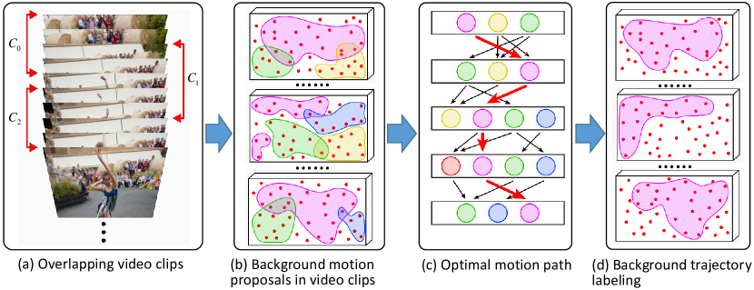
To describe the motions in the local clips, we use a set of epipolar geometries (EG) computed from neighboring video frames. Therefore, our method can effectively handle videos with large depth variation. Our method is much simpler compared to the existing motion segmentation techniques, since we are only concerned with the background motion and treat all other motions as foreground motions. Our motion estimation method is very fast, and the whole pipeline can run very efficiently even with densely sampled trajectories.
2 Related Work
While the aim of video object segmentation is to segment out the foreground objects from a video sequence, this approach can indeed be used to perform background extraction. However, many of these works require some degree of human intervention, such as the semi-supervised methods [1, 26, 8, 22, 21, 16] which require a small amount of manual annotation, and the fully-supervised methods [2, 31, 6] which require repeating result correction by the user. Our work is completely autonomous, like the unsupervised methods of video object segmentation [5, 11, 19, 27, 24, 29, 10]. However, the underlying assumption of our work is less brittle compared to those subscribed to by these works. For instance, [10, 29] rely on the ability of object proposals to detect the foreground objects; this might fail to work when the foreground objects have complex non-compact shapes. [19, 27] detect foreground objects by analysing the 2D motion field based on a simple assumption that they usually move differently from their surroundings. However, the 2D motions of some background objects may also have this property if the background has large depth variation.
Trajectory-based motion segmentation methods usually produce multiple independent motion groups; however, they usually stop short of actually identifying the background motion, or just use a simple background metric such as size. Furthermore, due to the computational demand of the 3D motion segmentation methods [25, 4, 12, 28], these works lack the ability to deal with large amount of feature trajectories. For long and densely sampled feature trajectories, some fast 2D methods [18, 9] may be used. However, their results may become over-segmented when the figure-ground is complex, for instance, scenes with large depth variation. Our method not only processes large amount of trajectory in an efficient way, but also handle videos with complex scene structures.
In addition to the above approaches, Bideau and Learned-Miller [3] proposed a probabilistic model to segment all the moving objects. Similar to many of the above approaches, their method cannot handle scenes with large foreground objects and may face difficulties when dealing with intermittent motions. Zhang et al.’s work [30] built a directed graph from local motion groups; this approach is closely related to ours. Our method is different from theirs in two aspects. Most importantly, we identify the background motion as the one with the largest amount of feature trajectories in the aggregate, while their method is based on the conjecture that the background trajectory matrix should exhibit a lower rank. This assumption is a serious qualification: it will not work if the foreground motions are also rigid. Another difference is that our method tries to find as many rigid motions as possible in each video clip, instead of committing to a clean segmentation for all the feature trajectories based on traditional motion segmentation methods. This allows us to recover from errors that might arise at the local clip levels.
3 Algorithm Overview
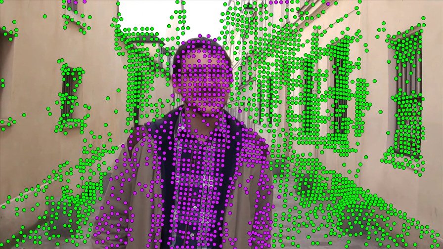
Given a dynamic video with large foreground objects, we first extract feature trajectories using the method [23]. We followed the instruction from [23] and used the author’s codes to generate the feature trajectories. Trajectories are extracted at a fixed interval in both horizontal and vertical directions. Our algorithm takes these trajectories as input and outputs those belong to the static background by estimating the dominant rigid motion in the video. The system pipeline is shown in Fig. 1.
The system first divides the input video into many short overlapping video clips of variable lengths, i.e.,, (Fig. 1 (a)). Inside each video clip , we propose multiple motion candidates , which contain different sizes of trajectory groups (Fig. 1 (b)). Each represents a rigid motion inside . The global background motion for the entire video is a collection of the background motions in these video clips, i.e., select one for each .
Since the background motions inside the video clips may not always be the majority one with the presence of large foreground objects, we identify it using a graph search method in a global manner (Fig. 1 (c)). Specifically, we construct a directed graph with in each as graph nodes. Directed edges are only created from nodes in to those in with shared trajectories. Among all the possible motion paths that start from the very first clip to the last one, we select the one that contains the largest amount of feature trajectories as our global background motion.
For objects with intermittent motions, i.e. they may be static in some video clips, their motions in those clips may be wrongly labeled as background. Therefore, we further perform a temporal consistency check and background motion refinement to rectify those wrongly labeled trajectories (Fig. 1 (d)).
4 Motion Estimation in Video Clips
Given a clip with time window , we divide the feature trajectories into three categories, i.e., . The indicator is set according to the following rules.
| (1) |
The indicator of a trajectory is set to if the trajectory lives throughout the entire time window (we call them full-length trajectories inside the time window), otherwise, it is set to or . This labeling of feature trajectories will be used to facilitate dividing the input video into overlapping video clips.
4.1 Video Clips Generation
Starting from the first video frame, we keep adding new frames to expand the time window of the first video clip as long as the number of the full-length feature trajectories inside , i.e. , is more than of all the visible trajectories inside it, as define below,
| (2) |
The next video clip starts from the middle frame of and expands in the same way. We repeat this process until the end of the video sequence is reached.
We experimentally set the ratio here to achieve a balance between enough camera movement within a clip and adequate trajectory overlap with the next video clip. As a result, long video clips will be generated when the camera movement is small. This ensures that even under small camera movement, there will always be enough motion cues within a particular clip for robust motion estimation.
4.2 Motion Model
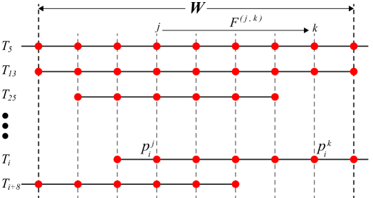
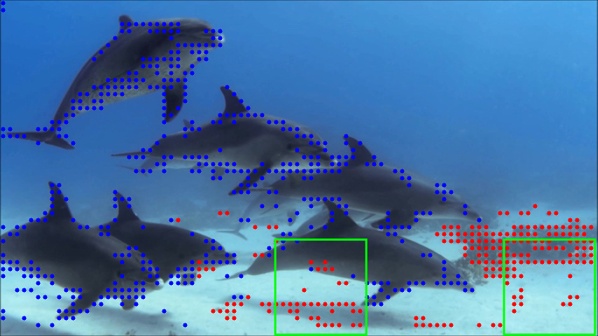
In our method, a rigid motion defined by a set of trajectories is represented by a series of fundamental matrices , where , are the video frame indices inside clip (see Fig. 2). Here, is empirically set to five as the feature tracking error is usually acceptable within this range for good fundamental matrix estimation. We estimate the fundamental matrix by applying the 8-point algorithm [7] on the feature matches extracted from these trajectories that are both visible at frames and .
To decide if a trajectory belongs to a known rigid motion , we compute its geometric errors based on the point-to-epipolar-line distance. Specifically, for each , if is both visible at frames and , we extract a feature match from it (see Fig. 2) and compute its geometric error with respect to as follows:
| (3) |
where and are all homogeneous coordinates and denotes the Euclidean point-to-line distance. If the error is smaller than a threshold ( in our implementation), we mark this feature match as a positive match. If more than of the tested feature matches from are marked as positive, we label as a member of the rigid motion.
4.3 Motion Estimation in Video Clips
Knowing that the background features may not constitute the majority in a video clip, we cannot hypothesize the background motion in the regular RANSAC fashion, i.e. randomly select eight full-length trajectories in RANSAC iterations. Instead, we adopt a local scanning scheme to effectively detect multiple motion candidates inside each clip.
For each video clip , we first divide the starting frame of into overlapping cells, e.g. overlap with a uniform size . For each cell, we collect the full-length trajectories inside it, and estimate a best-fitting motion in the regular RANSAC fashion. Specifically, in each RANSAC iteration, we randomly select eight full-length trajectories to compute a motion as described in Sec. 4.2. Then, we label the rest of the full-length trajectories inside the cell and count the inliers. If the inliers of the final best-fitting motion exceeds of all the full-length trajectories within that cell, we regard the estimated motion as a plausible background motion candidate for . Otherwise, it is discard. Note that we only use full-length trajectories here to ensure that we can compute a motion with a minimum eight trajectories.
After the RANSAC model fitting for all the single cells, we obtain a set of motion candidates . Since the background region may consist of several discrete parts across the image domain due to the large dynamic foreground motions and the estimated motions from single cells can be locally biased, we also perform the model fitting process on combinations of the single cells that yield . In our experiments, we find that combinations of up to three single cells are usually sufficient for robust background motion estimation. Eventually, successful motions from these combined cells together with those from the single cells form the final motion candidate set for
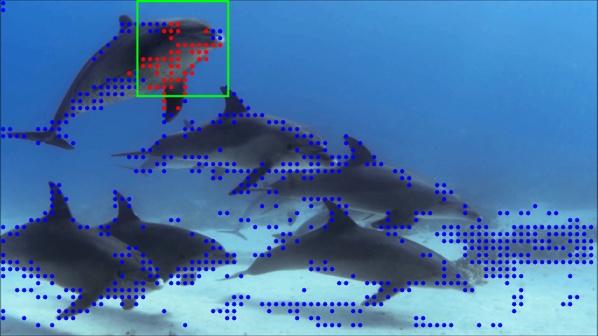
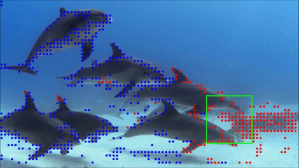
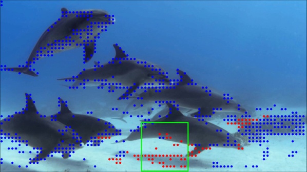
These motion candidates are estimated using full-length trajectories inside local cells. We still need to decide the membership of other trajectories inside the clip with respect to each of motion candidates. Fig. 3 shows some labeling results of the motion candidates. As we can see, unlike traditional motion segmentation methods that perform a clean segmentation of the trajectories and assign a unique label to each , our method usually generates multiple overlapping motion groups. Most importantly, since the motion candidates are estimated from densely overlapping cells, there is a high chance that the background will be the majority in at least one of these cells, and thus the true background motion can be estimated.
5 Dominant Motion Path Estimation
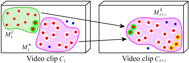
Once we obtain the motion candidates in each video clip, we construct a directed graph with these motion candidates as graph nodes (see Fig. 1 (c)). For two neighboring video clips and , we create a directed edge between two motion candidates if there exist some common trajectories between them, e.g. and in are both connected to in .
5.1 Graph Edge Weight
Among the multiple motion paths that traverse from the first video clip to the last, we now seek the optimal one that has the largest sum of trajectories along its path, i.e. the dominant rigid motion. A feature trajectory may live through multiple video clips and it may not always be the member of the motions along the path. For better trajectory counting along a motion path, we divide each into sub-trajectories, where is the number of video clips it spans. We then assign each sub-trajectory with a value of . With this simple normalization, we are now ready to count the number of trajectories in the following manner.
For an edge between and , an edge weight is defined as
| (4) |
where are the values of sub-trajectories common to both and , and are the values of those in that have newly appeared in . Therefore, we favor those strong connections, e.g. edge between and in Fig. 4 that have larger number of shared trajectories, because a consistent background motion path should have maximum overlapping trajectory groups.
is a weighting term that reflects the geometric error of a sub-trajectory under a certain motion candidate. It is defined as:
| (5) |
where , and is the average geometric error of trajectory under motion (see Eq. (3)). When a motion candidate is connected to multiple motions with similar number of shared trajectories, it will favor the connection with lower fitting error.
5.2 Optimal Path Search
Given a starting motion candidate in the first video clip and an ending one in , we estimate the optimal motion path from to that contains the largest number of trajectories by defining an objective function that maximizes the edge weights:
| (6) |
where is the set of connected edges from all motion candidates in to . When , we have , where is the sum of the sub-trajectories’ values inside , weighted by their corresponding geometric errors as in Eq. (4).
This optimal motion path searching problem between a motion candidate in to any other candidate in can be easily solved by dynamic programming. Finally, the global optimal motion path, starting from the first video clip to the last one, is selected by the following:
| (7) |
where is the total number of the video clips.
6 Background Trajectory Labeling
After obtaining the optimal motion path , i.e. background motion group, we label the sub-trajectories inside the selected motion candidates as background. Since a feature trajectory usually lives through multiple clips, and the optimal motion path may give its sub-trajectories different labels due to reasons like intermittent motion of the foreground objects or motion estimation errors, we need to perform a temporal consistency check for all the trajectories and use only reliable ones to compute the motion model of the global background motion.
Specifically, given the background motion path, we first identify reliable background feature trajectories that are entirely covered by the path, i.e. those whose all sub-trajectories are labelled as background. Then, we compute the global background motion model , using those reliable background trajectories as described in Sec. 4.2. Note that the time window of covers the entire video. Finally, we use to label all the feature trajectories in the video. And the labelled background trajectories will be the initial output of our algorithm.
6.1 Local Trajectory Label Filtering
Due to tracking errors, some background feature trajectories, especially those close to object boundaries, may be wrongly labeled as non-background trajectories, while most of its neighbors are correctly labeled. To obtain spatially-smooth but edge-preserving labeling results, we apply a local filtering process on the labeled trajectories based on their color similarity and spatial-temporal connectivity. Specifically, we regard two trajectories and as neighbors in the spatial-temporal domain if they have at least one shared video frame and their minimum distance inside these shared frames is less than a threshold ( of the frame width in our implementation). For each pair of such trajectory neighbors, we assign a weight to them, defined as follows:
| (8) |
where is the maximum distance between and inside their shared frames and is the average RGB color difference of them respectively. We set to of the frame width and in all our experiments.
If a feature trajectory is labeled as background initially, we assign a value to it. Otherwise, . The new label of is then determined by the following local filtering operation:
| (9) |
where is the set of trajectory neighbors of . If , we set the new label of as background. Otherwise, it is labeled as non-background trajectory. The filtering step produces the final results for background segmentation.
7 Experiments
We compare our method with several most recent state-of-the-art motion segmentation and background identification methods, which include the motion trajectory segmentation method [9], dense binary motion segmentation method [3], and the robust background identification method by Zhang et al. [30]. These methods represent different approaches for background identification tasks. The experiments are conducted with several well-known public datasets, where high quality ground truth foreground masks are provided. Specifically, we include FBMS-59 [18] (55 videos used), DAVIS [20] (32 videos used), Complex Background Data Set [17] (CBDS), Camouflaged Animals Data Set [3] (CADS), and the videos used in [30] for our analysis. These datasets contain various types of dynamic video (e.g. freely-moving camera, large depth variation, small foreground movement, highly dynamic scenes). Note that we discard some videos from FBMS-59 [18] and DAVIS [20] that violate the following criteria: (1) Available foreground mask should cover all the moving objects in the scenes. (2) The static background, regardless of its size, should always be visible. (3) No severe lens distortion in the video.
| Method | Precision (%) | Recall (%) | F-score | |||
| FBMS | DAVIS | FBMS | DAVIS | FBMS | DAVIS | |
| Keuper | 95.5 | 99.5 | 89.9 | 91.8 | 91.8 | 95.4 |
| Ours | 95.0 | 99.0 | 98.3 | 98.3 | 96.4 | 98.6 |
7.1 Comparison with Keuper et al. [9]
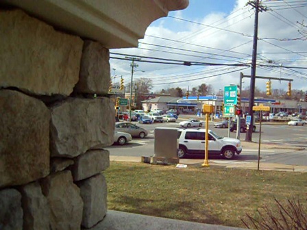
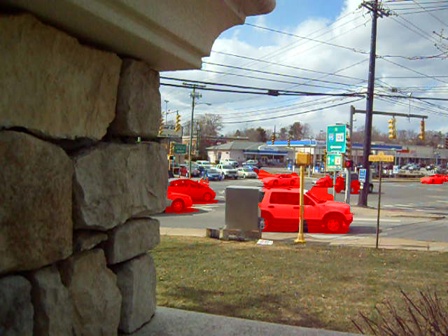
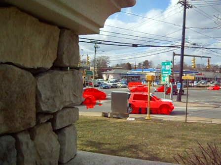
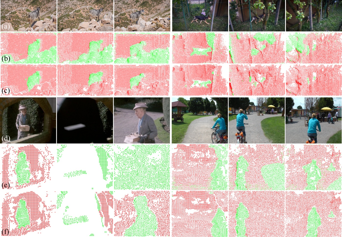
Keuper et al.’s method [9] is currently the state-of-the-art 2D motion segmentation method. To compare with their method, we test both methods on datasets FBMS-59 [18] and DAVIS [20]. The input feature trajectories are extracted by [23] for both methods. Since the output of [9] are multiple groups of feature trajectories, we select the one that contains the largest amount of trajectories and label the features inside as background. The comparison of average precision and recall for background features identification is shown in Tab. 1. As we can see from the table, our method achieves similar high accuracy as Keuper et al.’s method, while the recall of our method is significantly better. Fig. 5 shows some typical cases that may fail Keuper et al.’s method. Firstly, their method may not work well on scenes with large depth variation (top two cases in Fig. 5), which is a typical limitation of 2D motion segmentation methods without using a projective motion model. Secondly, when the background is severely occluded by the foreground moving objects (bottom left case in Fig. 5), their method may fail to track the background motion, and instead, creates new motion groups. Finally, since their method utilizes color information along with other motion cues in their energy function, it may over-segment the background region if it contains components with large color difference (bottom right case in Fig. 5). Our method, on the other hand, can very well handle such difficult cases.
7.2 Comparison with Bideau and Learned-Miller’s method [3]
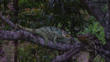
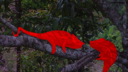
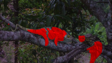
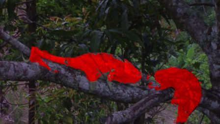
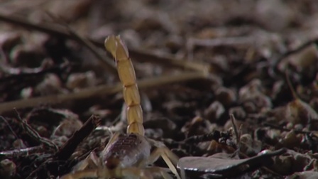
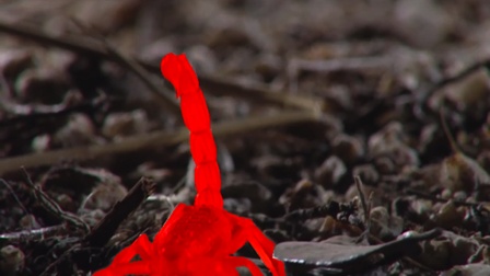
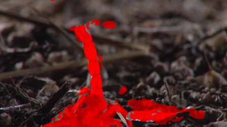
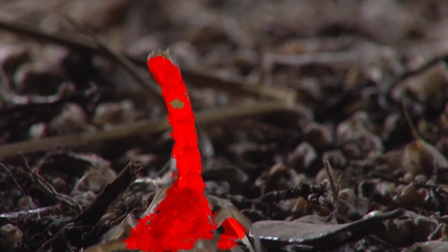
We also compare our method with Bideau and Learned-Miller’s method [3], which is a recent foreground object segmentation method. The datasets we use in this experiment are the Complex Background Data Set from [17] and the Camouflaged Animals Data Set from their own work. Since the main purpose of their method is segmenting foreground objects and the objects in these datasets are relatively small, we compute the precision and recall of pixels/features that locate on the foreground moving objects instead of background this time. The results are reported in Tab. 2. As we can see, in most cases, our method achieves better precision and recall. In general, our method produces more accurate and complete segmentation of the foreground objects, see examples in Fig. 6. The method proposed by [3], on the other hand, has difficulty dealing with foreground intermittent motions (‘chameleon’ sequence in Fig. 6), which are explicitly handled in our method by utilizing global motion cues.
7.3 Comparison with Zhang et al. [30]
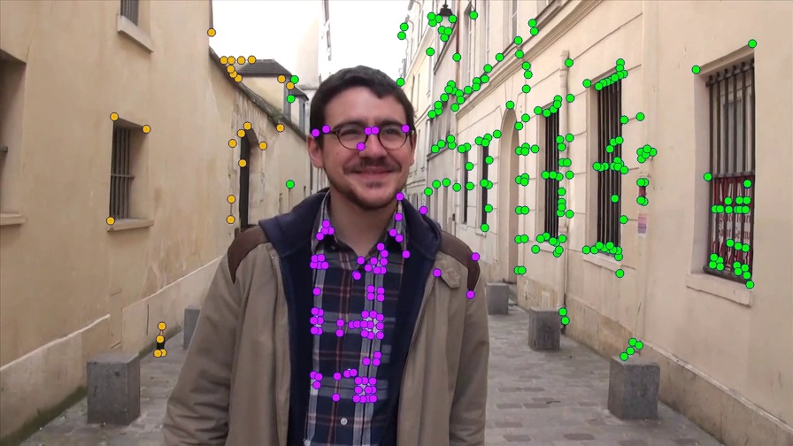
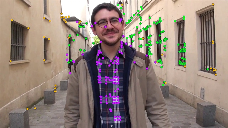
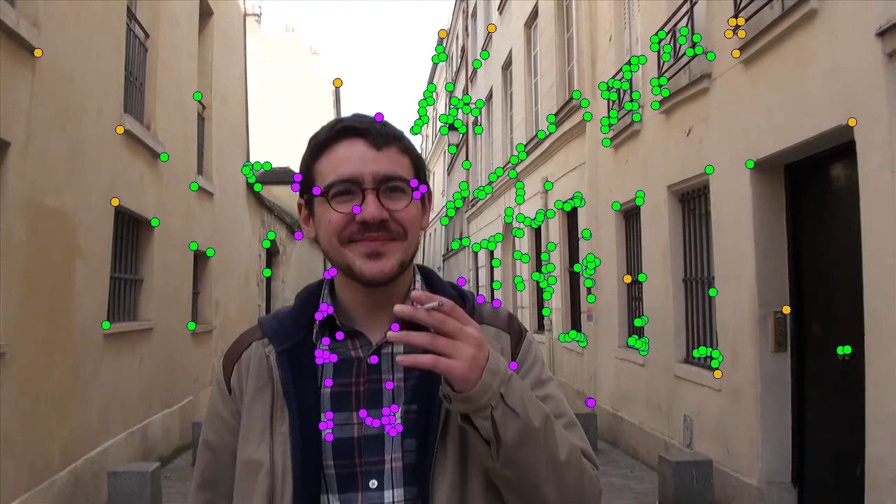
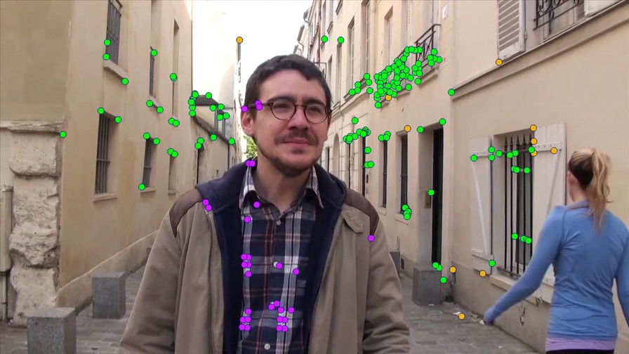
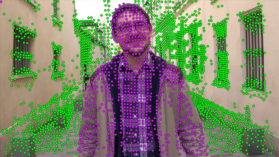
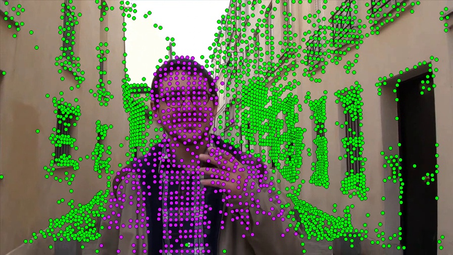
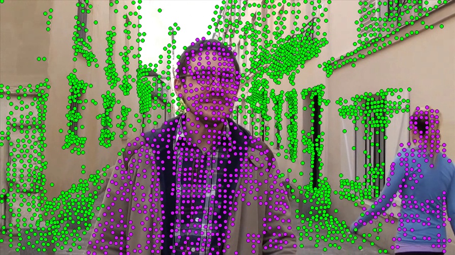
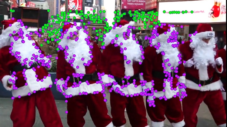
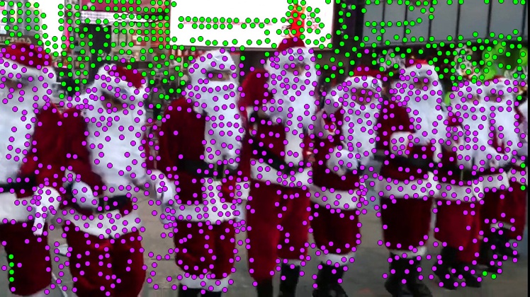
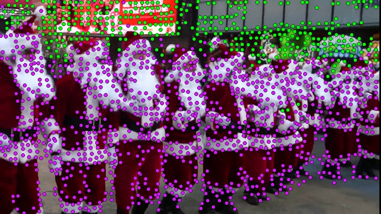
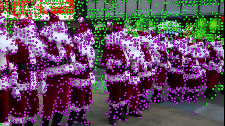
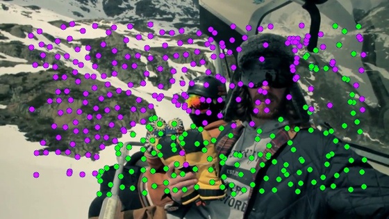
To evaluate the performance of our method on videos with large foreground objects, we compare our method with Zhang et al.’s method [30] on the highly dynamic videos used in their work. Some segmentation results are shown in Fig. 7. As we can see, our method can also produce very good segmentation results on these videos. Since we use projective motion model in our motion estimation step, the estimated background motion usually covers the entire background region. The motion segmentation method by Zhang et al. may produce over-segmented results as reported in their paper (yellow and green points on the background wall in Fig. 7 (a)). Therefore, it requires further post-processing to merge these background motion groups. Also, the background metric used in their method may be violated if the foreground motions are also rigid motions or nearly rigid motions (Fig. 7 (e)). Our background metric is based on the total number of feature trajectories a rigid motion contains in the entire video, which is proved to be more robust according to our experiment results.
| Sequence | Bideau [3] | Ours | |||
|---|---|---|---|---|---|
| preci. | recall | preci. | recall | ||
| CBDS [17] | ‘drive’ | 0.36 | 0.90 | 0.72 | 0.63 |
| ‘forest’ | 0.81 | 0.77 | 0.79 | 0.82 | |
| ‘parking’ | 0.897 | 0.89 | 0.902 | 0.92 | |
| ‘store’ | 0.91 | 0.78 | 0.94 | 0.84 | |
| ‘traffic’ | 0.73 | 0.83 | 0.83 | 0.85 | |
| CADS [3] | ‘chameleon’ | 0.96 | 0.53 | 0.94 | 0.66 |
| ‘frog’ | 0.49 | 0.38 | 0.50 | 0.40 | |
| ‘glowwormbeetle’ | 0.84 | 0.88 | 0.92 | 0.94 | |
| ‘scorpion1’ | 0.46 | 0.08 | 0.24 | 0.22 | |
| ‘scorpion2’ | 0.58 | 0.48 | 0.66 | 0.56 | |
| ‘scorpion3’ | 0.83 | 0.41 | 0.84 | 0.31 | |
| ‘scorpion4’ | 0.66 | 0.76 | 0.79 | 0.74 | |
| ‘snail’ | 0.95 | 0.90 | 0.98 | 0.86 | |
| ‘stickinsect’ | 0.06 | 0.17 | 0.20 | 0.31 | |
7.4 Limitations and Discussions
Our method may not work well in some special cases. Firstly, for videos with many short feature trajectories (only feature points on a trajectory) extracted from non-rigid objects like river and sea, where the features on these subtle dynamically moving objects may not violate the epipolar constraint during their short lifetime. Therefore, they may be wrongly labeled as background. Secondly, for videos captured by camera that hardly moves, if the foreground motion is also rigid and occupies the majority of the scene all the time (e.g. a video recorded by a standing person with a close-up view of a running train in front), our method may also fail to identify the correct background features. Computational wise, our method usually takes less than five minutes to process a video of around 100 frames and 50,000 trajectories on a PC with 2.4GHz CPU.
8 Conclusion
In this work, we propose a robust background feature identification method that can handle moving foreground objects that are large or exhibit intermittent motions. Our method is designed based on the assumption that the background motion will contain the largest amount of feature trajectories when the local background trajectories are aggregated over the entire sequence. Accordingly, we develop a local-to-global dominant motion group identification pipeline. Since the motions are characterized using fundamental matrices, there is no issue with over-segmentation, problem that plagues the 2D motion segmentation approach. With careful design, our motion estimation method can efficiently handle large amount of trajectories and robustly propose potential rigid motions in video clips. The comprehensive experiment results show that our method outperforms several most recent state-of-the-art motion segmentation methods both quantitatively and qualitatively.
References
- [1] Badrinarayanan, V., Galasso, F., Cipolla, R.: Label propagation in video sequences. In: Proc. CVPR (June 2010)
- [2] Bai, X., Wang, J., Simons, D., Sapiro, G.: Video snapcut: Robust video object cutout using localized classifiers. ACM Transactions on Graphics (2009)
- [3] Bideau, P., Learned-Miller, E.: It’s moving! a probabilistic model for causal motion segmentation in moving camera videos. In: European Conference on Computer Vision (ECCV) (2016)
- [4] Elhamifar, E., Vidal, R.: Sparse subspace clustering. In: Proc. CVPR. pp. 2790–2797 (2009)
- [5] Faktor, A., Irani, M.: Video segmentation by non-local consensus voting. In: BMVC (2014)
- [6] Fan, Q., Zhong, F., Lischinski, D., Cohen-Or, D., Chen, B.: Jumpcut: Non-successive mask transfer and interpolation for video cutout. ACM Transactions on Graphics (2015)
- [7] Hartley, R.I., Zisserman, A.: Multiple View Geometry in Computer Vision. Cambridge University Press, second edn. (2004)
- [8] Jain, S., Grauman, K.: Supervoxel-consistent foreground propagation in video. In: Proc. ECCV (2014)
- [9] Keuper, M., Andres, B., Brox, T.: Motion trajectory segmentation via minimum cost multicuts. In: Proc. ICCV (2015), http://lmb.informatik.uni-freiburg.de//Publications/2015/KB15b
- [10] Lee, Y.J., Kim, J., Grauman, K.: Key-segments for video object segmentation. In: Proc. ICCV (2011)
- [11] Li, F., Kim, T., Humayun, A., Tsai, D., Rehg, J.M.: Video segmentation by tracking many figure-ground segments. In: Proc. ICCV (2013)
- [12] Li, Z., Guo, J., Cheong, L.F., Zhiying Zhou, S.: Perspective motion segmentation via collaborative clustering. In: Proc. ICCV (December 2013)
- [13] Liu, S., Tan, P., Yuan, L., Sun, J., Zeng, B.: Meshflow: Minimum latency online video stabilization. In: ECCV. pp. 800–815. Springer (2016)
- [14] Liu, S., Yuan, L., Tan, P., Sun, J.: Bundled camera paths for video stabilization. ACM Trans. Graph. 32(4), 78:1–78:10 (Jul 2013)
- [15] Ma, Y., Derksen, H., Hong, W., Wright, J.: Segmentation of multivariate mixed data via lossy data coding and compression. IEEE Transactions on Pattern Analysis and Machine Intelligence 29(9), 1546–1562 (2007)
- [16] Maerki, N., Perazzi, F., Wang, O., Sorkine-Hornung, A.: Bilateral space video segmentation. In: Proc. CVPR (2016)
- [17] Narayana, M., Hanson, A., Learned-Miller, E.: Coherent motion segmentation in moving camera videos using optical flow orientations. In: Proc. ICCV. pp. 1577–1584 (2013)
- [18] Ochs, P., Malik, J., Brox, T.: Segmentation of moving objects by long term video analysis. IEEE Transactions on Pattern Analysis and Machine Intelligence (Jun 2014)
- [19] Papazoglou, A., Ferrari, V.: Fast object segmentation in unconstrained video. In: Proc. ICCV (December 2013)
- [20] Perazzi, F., Pont-Tuset, J., McWilliams, B., Gool, L.V., Gross, M., Sorkine-Hornung, A.: A benchmark dataset and evaluation methodology for video object segmentation. In: CVPR (2016)
- [21] Perazzi, F., Wang, O., Gross, M., Sorkine-Hornung, A.: Fully connected object proposals for video segmentation. In: Proc. ICCV (December 2015)
- [22] Ramakanth, S.A., Babu, R.V.: Seamseg: Video object segmentation using patch seams. In: Proc. CVPR (2014)
- [23] Sundaram, N., Brox, T., Keutzer, K.: Dense point trajectories by gpu-accelerated large displacement optical flow. In: Proc. ECCV (2010)
- [24] Taylor, B., Karasev, V., Scoatto, S.: Causal video object segmentation from persistence of occlusions. In: Proc. CVPR (2015)
- [25] Vidal, R., Tron, R., Hartley, R.: Multiframe motion segmentation with missing data using powerfactorization and gpca. International Journal of Computer Vision (2008)
- [26] Vijayanarasimhan, S., Grauman, K.: Active frame selection for label propagation in videos. In: Proc. ECCV (2012)
- [27] Wang, W., Shen, J., Porikli, F.: Saliency-aware geodesic video object segmentation. In: Proc. CVPR (2015)
- [28] Xu, X., Cheong, L.F., Li, Z.: Motion segmentation by exploiting complementary geometric models. In: Proc. CVPR (2018)
- [29] Zhang, D., Javed, O., Shah, M.: video object segmentation through spatially accurate and temporally dense extraction of primary object regions. In: Proc. CVPR (2013)
- [30] Zhang, F.L., Wu, X., Zhang, H.T., Wang, J., Hu, S.M.: Robust background identification for dynamic video editing. ACM Transactions on Graphics (2016)
- [31] Zhong, F., Qin, X., Peng, Q., Meng, X.: Discontinuity-aware video object cutout. ACM Transactions on Graphics (2012)
