An Efficient Algorithm for Enumerating Chordal Bipartite Induced Subgraphs in Sparse Graphs

Abstract

In this paper, we propose a characterization of chordal bipartite graphs and an efficient enumeration algorithm for chordal bipartite induced subgraphs. A chordal bipartite graph is a bipartite graph without induced cycles with length six or more. It is known that the incident graph of a hypergraph is chordal bipartite graph if and only if the hypergraph is $\beta$-acyclic. As the main result of our paper, we show that a graph $G$ is chordal bipartite if and only if there is a special vertex elimination ordering for $G$, called CBEO. Moreover, we propose an algorithm ECB which enumerates all chordal bipartite induced subgraphs in $O(kt\Delta^{2})$ time per solution on average, where $k$ is the degeneracy, $t$ is the maximum size of $K_{t,t}$ as an induced subgraph, and $\Delta$ is the degree. ECB achieves constant amortized time enumeration for bounded degree graphs.

1 Intorduction

A graph $G$ is chordal if any cycle with length four or more in $G$ has an edge, called a chord, which connects two nonconsecutive vertices on the cycle. If $G$ is a chordal, many NP-complete problems can be solved in polynomial time [Gavril:SIAM:1972]. Graph chordality is also interested in enumeration algorithm area. There are many efficient algorithms for enumerating subgraphs and supergraphs with chordality [Kiyomi:WG:2006, Kiyomi:IEICE:2006, Wasa:DS:2013, Daigo:SOFSEM:2009]. Moreover, chordality of a bipartite graph has been also well studied. A chordal bipartite graph is a bipartite graph without any induced cycles with length six or more. There are many characterizations of chordal bipartite graphs [Brandstadt:1999, Huang:JCT:2006, Uehara:ICALP:2002, Duris:IPL:2012]. In addition, the graph chordality is related to the hypergraph acyclicity [Beeri:JACM:1983, Brandstadt:1999]. In particular, Ausiello et al. show that a hypergraph is $\beta$-acyclic if and only if its bipartite incident graph is chordal bipartite.

A subgraph enumeration problem is defined as follows: To output all subgraphs satisfying a constraint. To evaluate the efficiency of enumeration algorithms, we often measure in terms of the size of input and the number of outputs. An enumeration algorithm is polynomial delay if the maximum interval between two consecutive solutions is polynomial. Moreover, an enumeration algorithm is amortized polynomial if the total running time is $O(M\cdot poly(N))$ time, where $M$ is the number of solutions, $N$ is the input size, and $poly$ is a polynomial function. In enumeration algorithm area, there are efficient algorithms for sparse graphs [Wasa:Arimura:Uno:ISAAC:2014, Wasa:COCOON:2018, Alessio:Roberto:ICALP:2016, Eppstein:Loffler:EXP:2013, Kante:Limouzy:FCT:2011, Kazuhiro:ISAAC:2018]. Especially, the degeneracy [Lick:CJM:1970] of graphs has been payed much attention for constructing efficient enumeration algorithms.

Main results: In this paper, we propose chordal bipartite induced subgraph enumeration algorithm ECB. In ECB, we use a similar strategy as enumeration of chordal induced subgraphs. Kiyomi and Uno [Kiyomi:IEICE:2006] use a special vertex ordering, called the perfect elimination ordering $(v_{1},\dots,v_{n})$. In this ordering, any vertex $v_{i}$ is simplicial in $G[V_{i:n}]$, where $V_{i:n}=\{v_{j}\in V\mid i\leq j\leq\}n$. Here, a vertex is called simplicial if an induced subgraph of neighbors becomes a clique. Kiyomi and Uno developed a constant delay enumeration algorithm for chordal induced subgraphs [Kiyomi:IEICE:2006] by using this ordering. Likewise a perfect elimination ordering of a chordal graph, we show that every chordal bipartite graph has a special vertex elimination ordering, and this is actually a necessary and sufficient condition of a chordal bipartite graph. We call this vertex ordering a chordal bipartite elimination ordering (CBEO). CBEO is defined by the following operation: Recursively remove a weak-simplicial vertex [Uehara:ICALP:2002]. Interestingly, CBEO is a relaxed version of a vertex ordering proposed by Uehara [Uehara:ICALP:2002]. By using CBEO, we propose our enumeration algorithm which outputs all chordal bipartite induced subgraphs in amortized $O(kt\Delta^{2})$ time, where $k$ is the degeneracy of a graph, $t$ is the maximum size of $K_{t,t}$ as an induced subgraph, and $\Delta$ is the degree of $G$. Note that $t$ is bounded by $k$. Hence, ECB enumerates chordal bipartite induced subgraphs in constant amortized time for bounded degree graphs.

2 Preliminaries

Let $G=(V,E)$ be a simple graph, that is there is no self loops and multiple edges. $u,v\in V$ are adjacent if there is an edge $\{u,v\}\in E$. The sequence of distinct vertices $\pi=(v_{1},\dots,v_{k})$ is a path if $v_{i}$ and $v_{i+1}$ are adjacent for each $1\leq i\leq k-1$. If $v_{1}=v_{k}$ holds in a path $C=(v_{1},\dots,v_{k})$, we call $C$ a cycle. The distance $dist(u,v)$ between $u$ and $v$ is defined by the length of a shortest path between $u$ and $v$. We call a graph $H=(U,F)$ a subgraph of $G=(V,E)$ if $U\subseteq V$ and $F\subseteq E$ hold. A subgraph $H=(U,F)$ is an induced subgraph of $G$ if $F=\{\{u,v\}\in E\mid u,v\in U\}$ hold. In addition, we denote an induced subgraph as $G[U]$. The neighbor of $v$ is the set of vertices $\{u\in V\mid\{u,v\}\in E\}$ and denoted by $N_{G}(v)$. If there is no confusion, we denote $N(v)$ as $N_{G}(v)$ In addition, we denote $N(v)\cap X$ as $N_{X}(v)$, where $X$ is a subset of $V$. The set of vertices $N[v]=N(v)\cup\{v\}$ is called the closed neighbor. We define the neighbor with distance $k$ and the neighbor with distance at most $k$ as $N^{k}(v)=\{u\in V\mid dist(u,v)=k\}$ and $N^{1:k}(v)=\bigcup_{1\leq i\leq k}N(v)^{k}$, respectively. $\mathcal{N}(v)$ is the neighbor set of neighbors defined as $\{N(u)\mid u\in N(v)\}$. The degree of $v$ $d(v)$ is the size of $N(v)$. The degree of a graph $G$ is the maximum size of $d(v)$ in $V$. Let $U$ be a subset of $V$. For vertices $u,v\in V$, $u$ and $v$ are comparable if $N(v)\subseteq N(u)$ or $N(v)\supseteq N(u)$ hold. Otherwise, $u$ and $v$ are incomparable.

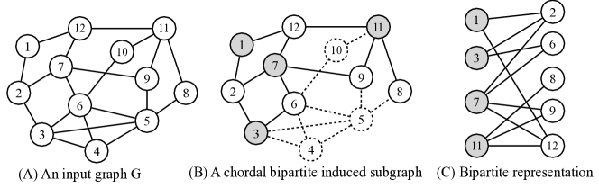
Figure 1: (A) shows an input graph $G$ and (B) shows one of the solutions $B=(X,Y,E)$, where $X=\{1,3,7,11\}$ and $Y=\{2,6,8,9,12\}$. (C) shows the graph $B$ drawn by dividing $X$ and $Y$.

Let $B=(X,Y,E)$ be a bipartite graph. We call $B$ is a chordal bipartite graph if there is no induced cycles with the length four or more. A bipartite graph $B$ is biclique if any pair of vertices $x\in X$ and $y\in Y$ are adjacent. We denote a biclique as $K_{a,b}$ if $\left|X\right|=a$ and $\left|Y\right|=b$. In this paper, we consider only the case $a=b$ and the size of a biclique $K_{t,t}$ is $t$.

Let $\mathcal{H}=(V,\mathcal{E})$ be a hypergraph, where $V$ is a set of vertices and $\mathcal{E}$ is a set of subsets of $V$. We call an element of $\mathcal{E}$ a hyperedge. For a vertex $v$, let $\mathcal{H}(v)$ be the set of edges $\{e\in\mathcal{H}\mid v\in e\}$ which contain $v$. A sequence of edges $C=(e_{1},\dots,e_{k})$ is a berge cycle if there exists $k$ distinct vertices $v_{1},\dots,v_{k}$ such that $v_{k}\in e_{1}\cap e_{k}$ and $v_{i}\in e_{i}\cap e_{i+1}$ for each $1\leq i<k$. A berge cycle $C=(e_{1},\dots,e_{k})$ is a pure cycle if $k\geq 3$ and $e_{i}\cap e_{j}\neq\emptyset$ hold for any distinct $i$ and $j$, where $i$ and $j$ satisfy one of the following three conditions: (I) $|i-j|=1$, (II) $i=1$ and $j=k$, or (III) $i=k$ and $j=1$. A cycle $C=(e_{1},\dots,e_{k})$ is a $\beta$-cycle if the sequence of $(e^{\prime}_{1},\dots,e^{\prime}_{k})$ is a pure cycle, where $e^{\prime}_{i}=e_{i}\setminus\bigcap_{1\leq j\leq k}e_{j}$. We call a hypergraph $\mathcal{H}$ $\beta$-acyclic if $\mathcal{H}$ has no $\beta$-cycles. We call a vertex $v$ a $\beta$-leaf (or nest point) if $e\subseteq f$ or $e\supseteq f$ hold for any pair of edges $e,f\in\mathcal{H}(v)$. A bipartite graph $\mathcal{I}(\mathcal{H})=(X,Y,E)$ is a incidence graph of a hypergraph $\mathcal{H}=(V,\mathcal{E})$ if $X=V$, $Y=\mathcal{E}$, and $E$ includes an edge $\{v,e\}$ if $v\in e$, where $v\in V$ and $e\in\mathcal{E}$. $\mathcal{V}$ is totally ordered if for any pair $X,Y\in\mathcal{V}$ of vertex subsets, either $X\subseteq Y$ or $X\supseteq Y$. we assume that $\mathcal{H}$ is not trivial, that is, $\mathcal{H}$ has more than one vertex.

Finally, we define our problem, chordal bipartite induced subgraph enumeration problem. In Fig. 1, we show an input graph $G$ and one of the solutions.

Problem 1 (Chordal bipartite induced subgraph enumeration problem).

Output all chordal induced subgraphs in an input graph $G$ without duplication.

3 A Characterization of Chordal Bipartite Graphs

We propose a new characterization of chordal bipartite graphs. By using this characterization, we construct a proposed algorithm in Sect. 4. We first give notions. A vertex $v$ is weak-simplicial [Uehara:ICALP:2002] if $N(v)$ is an independent set and any pair of neighbors of $v$ are comparable. A bipartite graph $B=(X,Y,E)$ is bipartite chain if any pair of vertices in $X$ or $Y$ are comparable, that is, $N(u)\subseteq N(v)$ or $N(u)\supseteq N(v)$ holds for any $u,v\in X$ or $u,v\in Y$. To show the new characterization, we use the following two theorems.

Theorem 1 (Theorem 1 of [Ausiello:JCS:1986] ).

$\mathcal{I}(\mathcal{H})$ is chordal bipartite if and only if $\mathcal{H}$ is $\beta$-acyclic.

Theorem 2 (Theorem 3.9 of [Brault:ACM:2016]).

A $\beta$-acyclic hypergraph $\mathcal{H}=(\mathcal{V},\mathcal{E})$ with at least two vertices has two distinct $\beta$-leaves that are not neighbors in $\mathcal{H^{\prime}}=(\mathcal{V},\mathcal{E}\setminus\{\mathcal{V}\})$.

Brault [Brault:ACM:2016] gives a vertex elimination ordering $(v_{1},\dots,v_{n})$ for a hypergraph $\mathcal{H}$, called a $\beta$-elimination ordering. The definition is as follows: For any $1\leq i\leq n$, $v_{i}$ is a $\beta$-leaf in $\mathcal{H}[V_{i:n}]$, where $V_{i:n}=\{v_{j}\in V\mid i\leq j\leq n\}$. It is known that $\mathcal{H}$ is $\beta$-acyclic if and only if there is a $\beta$-elimination ordering of $\mathcal{H}$. Similarly, in this paper, for any graph $G$, we define a vertex elimination ordering $(v_{1},\dots,v_{n})$ for $G$, called CBEO, as follows: for any $1\leq i\leq n$, $v_{i}$ is a weak-simplicial in $G[V_{i:n}]$. In the remaining of this section, we show that a graph is chordal bipartite if and only if there is CBEO for $G$. Lemma 3 shows that a $\beta$-leaf of a hypergraph is weak-simplicial in its incident graph.

Lemma 3.

Let $\mathcal{H}=(\mathcal{V},\mathcal{E})$ be a hypergraph, $v$ be a vertex in $\mathcal{V}$, and $v^{\prime}$ be the corresponding vertex of $v$ in $X$ of $\mathcal{I}(\mathcal{H})$. Then, $v$ is a $\beta$-leaf in $\mathcal{H}$ if and only if $v^{\prime}$ is a weak-simplicial vertex in $\mathcal{I}(\mathcal{H})$.

Proof.

We assume that $v$ is a $\beta$-leaf in $\mathcal{H}$. Let $v^{\prime}$ be the vertex corresponding to $v$ in $\mathcal{I}(\mathcal{H})$. From the definition of a $\beta$-leaf, $\mathcal{N}(v)$ is also totally ordered in $\mathcal{I}(\mathcal{H})$. Thus, $v$ is a weak-simplicial vertex in $\mathcal{I}(\mathcal{H})$.

We next assume that $v^{\prime}$ is weak-simplicial in $X$ of $\mathcal{I}(\mathcal{H})$. From the definition, $\mathcal{N}(v)$ is totally ordered. Thus, $\mathcal{H}(v)$ is totally ordered. Therefore, $v$ is a $\beta$-leaf in $\mathcal{H}$ and the statement holds. ∎∎

From Lemma 3, a $\beta$-leaf $v$ of $\mathcal{H}$ corresponds to a weak-simplicial vertex of an incident graph $\mathcal{I}(\mathcal{H})$. We next show that a chordal bipartite graph has at least one weak-simplicial vertex from Theorem 1, Theorem 2, and Lemma 3.

Lemma 4.

Let $B=(X,Y,E)$ be a chordal bipartite graph with at least two vertices. If there is no vertex $v$ in $B$ such that $N(v)=X$ or $N(v)=Y$, then $B$ has at least two weak-simplicial vertices which are not adjacent.

Proof.

From Theorem 1, Theorem 2, and Lemma 3, if $B$ is chordal bipartite and has no twins, then $G$ has at two weak-simplicial vertices which are not adjacent. We now assume $B$ has twins. We construct $B^{\prime}$ as follows: For each set of twins $T\in\mathcal{T}$, remove all vertices in $T$ except one twin of $T$, where $\mathcal{T}$ is the sets of twins of $B$. Note that $B^{\prime}$ is still chordal bipartite since vertex deletion does not destroy the chordality. Since $B^{\prime}$ has no twins, $B^{\prime}$ has at least two weak-simplicial vertices $u$ and $v$ which are not adjacent. Since the set inclusion relation between $B$ and $B^{\prime}$ is same, $u$ and $v$ also weak-simplicial in $B$. Hence, the statement holds. ∎∎

Theorem 5.

Let $B$ be a bipartite graph. $B$ is chordal bipartite if and only if there is a CBEO for $B$.

Proof.

From Lemma 4, the only if part holds. We consider the contraposition of the if part. Suppose that $B$ is not chordal bipartite. Then, $B$ has an induced cycle $C$ with length six or more. Since a vertex in $C$ is not weak-simplicial, we cannot eliminate all vertices from $B$ and the statement holds. ∎∎

We next show that a vertex $v$ is weak-simplicial in a bipartite graph $B$ if and only if $B[N^{1:2}(v)]$ is bipartite chain.

Lemma 6.

Let $B=(X,Y,E)$ be a chordal bipartite graph and $v$ be a vertex in $B$. Then, $v$ is weak-simplicial if and only if an induced subgraph $B[N^{1:2}[v]]$ is bipartite chain.

Proof.

We assume that $B[N^{1:2}[v]]$ is bipartite chain. From the definition, any pair of vertices in $N(v)$ are comparable. Hence, $v$ is weak-simplicial.

We next prove the other direction. We assume that $v$ is weak-simplicial. Let $x$ and $y$ be vertices in $N^{2}(v)$. If $x$ and $y$ are incomparable in $B[N^{\leq 2}[v]]$, then there are two vertices $z\in N(x)\setminus N(y)$ and $z^{\prime}\in N(y)\setminus N(x)$. Note that $z$ and $z^{\prime}$ are neighbors of $v$. This contradicts that any pair of vertices in $N(v)$ are comparable. Hence, $x,y\in N^{2}(v)$ are comparable and $B[N^{\leq 2}[v]]$ is bipartite chain. ∎∎

4 Enumeration of Chordal Bipartite Induced Subgraphs

1 Procedure ECB($G$) // $G=(V,E)$: an input graph

2       RecECB($(\emptyset,\emptyset,V,G)$);

3      

4Procedure RecECB($X,WS(X),AWS(X),G$)

5       Output $X$ and Compute $C\left(X\right)$ from $AWS(X)$;

6       for $v\in C\left(X\right)$ do

7             $Y\leftarrow X\cup\{v\}$;

8             if $\mathcal{P}\left(Y\right)=X$ then  RecECB($Y,WS(Y),AWS(Y),G$) ;

9            

Algorithm 1 ECB enumerates all chordal bipartite induced subgraphs in amortized polynomial time.

In this section, we propose an enumeration algorithm ECB for chordal bipartite subgraphs based on reverse search [Avis:Fukuda:DAM:1996]. ECB enumerates all solutions by traversing on a tree structure $\mathcal{F}\left(G\right)=(\mathcal{S}(G),\mathcal{E}(G))$, called a family tree, where $\mathcal{S}(G)$ is a set of solutions in an input graph $G$ and $\mathcal{E}(G)\subseteq\mathcal{S}(G)\times\mathcal{S}(G)$. Note that $\mathcal{F}\left(G\right)$ is directed. We give $\mathcal{E}(G)$ by defining the parent-child relationship among solutions based on Theorem 5.

Let $X$ be a vertex subset that induces a solution. We denote the set of weak-simplicial vertices in $G[X]$ as $WS(X)$. In what follows, we number the vertex index from $1$ to $n$ and compare the vertices with their indices. The parent of $X$ is defined as $\mathcal{P}\left(X\right)=X\setminus\mathop{\rm arg~{}max}\limits{WS(X)}$. $X$ is a child of $Y$ if $\mathcal{P}\left(X\right)=Y$. Let $ch(X)$ be the set of children of $X$. We define the parent vertex $pv(X)$ as $\mathop{\rm arg~{}max}\limits{WS(X)}$ which induces the parent. For any pair of solutions $X$ and $Y$, $(X,Y)\in\mathcal{E}(G)$ if $Y=\mathcal{P}\left(X\right)$. From Theorem 5, any solution can reach the empty set by recursively removing the parent vertex from the solution. Hence, the following lemma holds.

Lemma 7.

The family tree forms a tree.

Next, we show that ECB enumerates all solutions. For any vertex subset $X\subset V$, we denote $X_{1:i}=X\cap V_{1:i}$. An addible weak-simplicial vertex set is $AWS(X)=\{v\in V\setminus X\mid v\in WS(X\cup\{v\})\}$, that is, any vertex $v$ in $AWS(X)$ generates new solution $X\cup\{v\}$. We define a candidate set $C\left(X\right)$ as follows: $C\left(X\right)=AWS(X)_{pv(X):n}\cup(AWS(X)\cap N^{1:2}(pv(X)))$. Note that $C\left(X\right)$ is a subset of $AWS(X)$. We show that the relation between $ch(X)$ and $C\left(X\right)$.

Lemma 8.

Let $X$ and $Y$ be distinct solutions. If $Y$ is a child of $X$, then $pv(Y)\in C\left(X\right)$.

Proof.

Suppose that $Y$ is a child of $X$. Let $v=pv(Y)$ and $u=pv(X)$. Note that $v$ belongs to $AWS(X)$. If $u<v$, then $v\in AWS_{u:n}(X)$ and thus $v\in C\left(X\right)$. Otherwise, $u$ is not included in $WS(Y)$ since $v$ has the maximum index in $WS(Y)$. From the definition of a weak-simplicial vertex, there are two vertices in $N_{Y}(u)$ which are incomparable in $G[Y]$. Since $\mathcal{N}(u)$ is totally ordered in $G[X]$, $v$ must be in $N^{1:2}(u)$. Hence, the statement holds. ∎∎

In what follows, we call a vertex $v\in C\left(X\right)$ generates a child if $X\cup\{v\}$ is a child of $X$. From Lemma 7 and Lemma 8, ECB enumerates all solution by the DFS traversing on $\mathcal{F}\left(G\right)$.

Theorem 9.

ECB enumerates all solutions.

5 Time complexity analysis

1 Procedure UpdateWS($X,v,WS(X),G$)

2       $WS\leftarrow WS(X)$;

3       for $u\in N_{X}(v)$ do

4             if $u\in WS\land$ there is a vertex $w\in N_{X}(u)$ is incomparable to $u$.  then $WS\leftarrow WS\setminus\{u\}$;

5             for $w\in N_{X}(u)\cap WS$ do

6                   if $w$ and $v$ are incomparable then  $WS\leftarrow WS\setminus\{w\}$ ;

7                  

8      return $WS$;

9      

10Procedure UpdateAWS($X,v,AWS(X),G$)

11       $AWS\leftarrow AWS(X)$;

12       for $u\in N(v)$ do

13             if $u\in AWS$ then

14                   if There is a vertex $w\in N_{X}(u)$ which is incomparable to $u$.  then $AWS\leftarrow AWS\setminus\{u\}$;

15                  

16            else if $u\in X$ then

17                   for $w\in N(u)\cap AWS$ do

18                         if $w$ and $v$ are incomparable.  then  $AWS\leftarrow AWS\setminus\{w\}$ ;

19                        

20      return $AWS$;

21      

Algorithm 2 UpdateWS and UpdateAWS are efficient functions to compute $WS(Y)$ and $AWS(Y)$ by using $WS(X)$ and $AWS(X)$, respectively.

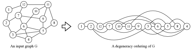
Figure 2: It is a degeneracy ordering of $G$. The degeneracy of $G$ is three. In this ordering, $\left|N^{\leq 2}_{1:v}(v)\right|$ is at most $k\Delta$ for any vertex $v$.

ECB has two bottlenecks. (1) Some vertices in $C\left(X\right)$ does not generate a child and (2) the maintenance of $WS(X)$ and $AWS(X)$ consumes time. A trivial bound of the number of redundant vertices in $C\left(X\right)$ is $O(\Delta^{2})$ since only vertices in $(AWS(X)\cap N^{1:2}(pv(X))$ may not generate a child. To evaluate the number of such redundant vertices precisely, we use a degeneracy ordering. A graph $G$ is $k$-degenerate if any induced subgraph of $G$ has a vertex with degree $k$ or less [Lick:CJM:1970]. The degeneracy of a graph is the smallest such number $k$. Matula et al. [Matula:Beck:JACM:1983] show that a $k$-degenerate graph $G$ has a following vertex ordering: For each vertex $v$, the number of neighbors smaller than $v$ is at most $k$. This ordering is called a degeneracy ordering of $G$ (See Fig. 2). Matula et al. also show that a linear time algorithm for obtaining one of the orderings. In what follows, we fix a reverse order of a degeneracy ordering and $WS(X)$ and $AWS(X)$ are sorted in this ordering. We first show that the number of redundant vertices is at most $2k\Delta$.

Lemma 10.

Let $X$ be a solution. The number of vertices in $C\left(X\right)$ which do not generate a child is at most $2k\Delta$.

Proof.

Let $v$ be a vertex in $C\left(X\right)$ and $p$ be a vertex $pv(X)$. If $p<v$, then $v$ generates a child. We assume that $v<p$. Since $v$ is in $C\left(X\right)$, $v\in N^{1:2}(p)\cap AWX_{1:p}(X)$. We estimate the size of $N^{1:2}(p)\cap AWX_{1:p}(X)$. We consider a vertex $u\in N_{1:v}(v)$. $\sum_{u\in N_{1:v}(v)}\left|N(u)\right|$ is at most $k\Delta$ since $\left|N_{1:v}(v)\right|$ is at most $k$. We next consider a vertex $u\in N_{v:n}(v)$. Since $u$ is larger than $v$, a vertex in $N_{u:n}(u)$ is larger than $v$. Hence, we consider vertices $N_{1:u}(u)$. For each $u$, $\left|N_{1:u}(u)\right|$ is at most $k$. Hence, $\sum_{u\in N_{v:n}(v)}\left|N(u)_{1:u}\right|$ is at most $k\Delta$ and the statement holds. ∎∎

We next show how to compute $C\left(Y\right)$ from $C\left(X\right)$, where $X$ is a solution and $Y$ is a child of $X$. From the definition of $C\left(X\right)$, we can compute $C\left(Y\right)$ in $O(\left|C\left(Y\right)\right|+k\Delta)$ time if we have $AWS(Y)$ and $pv(Y)$. Moreover, if we have $WS(X\cup\{v\})$, then we can determine whether $X\cup\{v\}$ is a child of $X$ or not in constant time since $WS(X\cup\{v\})$ is sorted. Hence, to obtain children of $X$, computing $AWS(X)$ and $WS(X)$ dominate the computation time of each iteration. Here, we define two vertex sets as follows:

$$Del_{\text{W}}\left(X,v\right) =\{u\in N^{1:2}(v)\cap WS(X)\mid u\notin WS(X\cup\{v\})\}\text{ and }$$

$$Del_{\text{A}}\left(X,v\right) =\{u\in N^{1:2}(v)\cap AWS(X)\mid u\notin WS(X\cup\{u,v\})\}.$$

These vertex sets are the sets of vertices that are removed from $WS(X)$ and $AWS(X)$ after adding $v$ to $X$, respectively. In the following lemmas, we show that $WS(X)$ and $AWS(X)$ can be update if we have $Del_{\text{W}}\left(X,v\right)$ and $Del_{\text{A}}\left(X,v\right)$.

Lemma 11.

Let $X$ be a solution, $Y$ be a child of $X$, and $v=pv(Y)$. Then, $WS(Y)=(WS(X)\setminus Del_{\text{W}}\left(X,v\right))\cup\{v\}$.

Proof.

Let $u$ be a vertex in $WS(Y)$. We prove $u$ is included in $(WS(X)\setminus Del_{\text{W}}\left(X,v\right))\cup\{v\}$. If $u=v$ holds, then $u\in WS(Y)$ since $v\in pv(Y)$. We assume that $u\neq v$. Since $u$ is weak-simplicial in $Y$, $u\in WS(X)$. If $u\in Del_{\text{W}}\left(X,v\right)$, then $u$ is not weak-simplicial in $Y$. It contradicts the assumption. Hence, $u\not\in Del_{\text{W}}\left(X,v\right)$. We prove the other direction. Let $u$ be a vertex in $(WS(X)\setminus Del_{\text{W}}\left(X,v\right))\cup\{v\}$. We assume that $u\neq v$. If $u\not\in WS(Y)$, then $u\in Del_{\text{W}}\left(X,v\right)$. It is contradiction and the statement holds. ∎

Lemma 12.

Let $X$ be a solution, $Y$ be a child of $X$, and $v=pv(Y)$. Then, $AWS(Y)=AWS(X)\setminus Del_{\text{A}}\left(X,v\right)$.

Proof.

Let $u$ be a vertex in $AWS(Y)$. We prove $u$ is included in $AWS(X)\setminus Del_{\text{A}}\left(X,v\right)$. From the definition of $AWS(X)$, $u\in AWS(X)$ holds. If $u\in Del_{\text{A}}\left(X,v\right)$, then $u$ is not weak-simplicial in $Y\cup\{u\}$. Since $u\in AWS(Y)$, $u\not\in Del_{\text{A}}\left(X,v\right)$. We prove the other direction. Let $u$ be a vertex in $AWS(X)\setminus Del_{\text{A}}\left(X,v\right)$. From the definition of $AWS(X)$ and $Del_{\text{A}}\left(X,v\right)$, $u$ is weak-simplicial in $X\cup\{v,u\}$. Hence, $u\in AWS(Y)$ and the statement holds. ∎∎

Note that by just removing redundant vertices, $WS(Y)$ and $AWS(X)$ can be easily sorted if $WS(X)$ and $AWS(X)$ were already sorted. We next consider how to compute $Del_{\text{W}}\left(X,v\right)$ and $Del_{\text{A}}\left(X,v\right)$. We first show a characterization of a vertex in $Del_{\text{W}}\left(X,v\right)$ and $Del_{\text{A}}\left(X,v\right)$. In the following lemmas, let $X$ be a solution, $v$ be a vertex in $AWS(X)$, and $Y$ be a solution $X\cup\{v\}$.

Lemma 13.

Let $u$ be a vertex in $N_{Y}(v)\cap WS(X)$. $u\in Del_{\text{W}}\left(X,v\right)$ if and only if $N_{X}(u)$ includes $w$ which is incomparable to $v$.

Proof.

If $u$ has a neighbor $w$ in $X$ which is incomparable to $v$, then from the definition, $u$ is not weak-simplicial.

Let $u$ be a vertex in $Del_{\text{W}}\left(X,v\right)$. There is a pair of vertices $w_{1}$ and $w_{2}$ in $N_{Y}(u)$ which are incomparable. If $w_{1}$ or $w_{2}$ is equal to $v$, then the statement holds. Hence, we assume that both $w_{1}$ and $w_{2}$ are not equal to $v$. Since $G[Y]$ is bipartite, $w_{1}$ and $w_{2}$ are not adjacent to $v$. Hence, $N_{X}(w_{1})=N_{Y}(w_{1})$ and $N_{X}(w_{2})=N_{Y}(w_{2})$ hold. It contradicts that $X$ is a solution and the statement holds. ∎∎

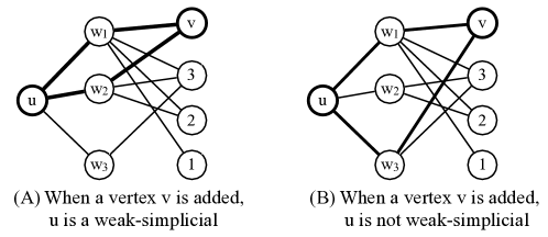
Figure 3: Let $X$ be a set of vertices $\{u,w_{1},w_{2},w_{3},1,2,3\}$. In $G[X]$, $L(X,u)=(w_{1},w_{2},w_{3})$. In case (A), a vertex $u$ is still weak-simplicial. In case (B), however, $u$ is not weak-simplicial since $N(v)$ includes only $w_{1}$ and $w_{3}$.

Lemma 14.

Let $u$ be a vertex in $N^{2}_{Y}(v)\cap WS(X)$. Then, $u\in Del_{\text{W}}\left(X,v\right)$ if and only if there exists a pair of vertices $w_{1},w_{2}\in N_{X}(u)$ which satisfy $N_{X}(w_{1})\subset N_{X}(w_{2})$, $v\in N_{Y}(w_{1})$, and $v\not\in N_{Y}(w_{2})$.

Proof.

The if part is easily shown by the assumption of the incomparability of $w_{1}$ and $w_{2}$. We next prove the other direction. We assume that $u\in Del_{\text{W}}\left(X,v\right)$. Hence, there is a pair of neighbors $w_{1}$ and $w_{2}$ of $u$ such that they are incomparable in $Y$. Without loss of generality, $N_{X}(w_{1})\subset N_{X}(w_{2})$ holds since $u$ is in $WS(X)$. If $N_{X}(w_{1})=N_{X}(w_{2})$, then $w_{1}$ and $w_{2}$ are comparable in $Y$. Since $w_{1}$ and $w_{2}$ are incomparable in $Y$, $w_{1}$ is adjacent to $v$ and $w_{2}$ is not adjacent to $v$. Thus, the statement holds. ∎∎

Lemma 15.

Let $u$ be a vertex in $N(v)\cap AWS(X)$ and $Z=X\cup\{u,v\}$. Then, $u\in Del_{\text{A}}\left(X,v\right)$ if and only if $u$ has a neighbor $w$ in $Z$ which is incomparable to $v$.

Proof.

The if part is trivial from the definition of weak-simplicial. We prove the only if part. We assume that $u\in Del_{\text{A}}\left(X,v\right)$ holds. Since $u\in Del_{\text{A}}\left(X,v\right)$, $u$ has a pair of neighbors $w_{1}$ and $w_{2}$ which are incomparable in $Z$. If $w_{1}$ or $w_{2}$ is equal to $v$, then $u$ has a neighbor $w$ which is incomparable to $v$ and the statement holds. We next assume that $w_{1}$ and $w_{2}$ are distinct from $v$. $v$ is not adjacent to $w_{1}$, $w_{2}$, or both of them since $G[Y]$ is bipartite. Hence, $w_{1}$ and $w_{2}$ are comparable in $Z$ since $w_{1}$ and $w_{2}$ are comparable in $G[X]$. This contradicts that $w_{1}$ and $w_{2}$ are incomparable in $Z$ and the statement holds. ∎∎

Lemma 16.

Let $u$ be a vertex in $N^{2}(v)\cap AWS(X)$ and $Z=X\cup\{u,v\}$. Then, $u\in Del_{\text{A}}\left(X,v\right)$ if and only if there exists a pair of vertices $w_{1},w_{2}\in N_{Z}(u)$ which satisfy $N_{Z}(w_{1})\subset N_{Z}(w_{2})$, $v\in N_{Z}(w_{1})$, and $v\not\in N_{Z}(w_{2})$.

Proof.

From the assumption, $w_{1}$ and $w_{2}$ are incomparable in $Z$. Hence, the if part holds. We prove the other direction. We assume that $u\in Del_{\text{A}}\left(X,v\right)$. Hence, $u$ has a pair of vertices $w^{\prime}_{1}$ and $w^{\prime}_{2}$ which are incomparable in $Z$. Without loss of generality, $N_{X\cup\{u\}}(w^{\prime}_{1})\subset N_{X\cup\{u\}}(w^{\prime}_{2})$ holds. Since $w^{\prime}_{1}$ and $w^{\prime}_{2}$ are incomparable in $G[Z]$, $w^{\prime}_{1}$ is adjacent to $v$. Thus, the statement holds. ∎∎

Next, we consider the time complexity of computing $Del_{\text{W}}\left(X,v\right)$ and $Del_{\text{A}}\left(X,v\right)$. For analysing these computing time more precisely, we give two upper bounds with respect to the number of edges and the size of $N^{2}(v)$ in bipartite chain graphs. Note that $t$ is the maximum size of $K_{t,t}$ in $B$ as an induced subgraph.

Lemma 17.

Let $B$ be a bipartite chain graph and $v$ be a vertex in $B$. Then, $\left|N^{2}(v)\right|$ is at most $\Delta$.

Proof.

Let $u$ be a maximum vertex in $N(v)$ with respect to inclusion of neighbors. Hence, for any vertex $w\in N(v)$, $N(w)\subseteq N(u)$ holds. Since $N^{2}(v)=\bigcup_{w\in N(v)}N(w)$, $N^{2}(v)$ is equal to $N(u)$. Hence, the statement holds. ∎∎

Lemma 18.

Let $B=(X,Y,E)$ be a bipartite chain graph. Then, the number of edges in $B$ is $O(t\Delta)$, where $t$ is the maximum size of a biclique in $B$.

Proof.

Let $v$ be a maximum vertex in $X$ with respect to inclusion of neighbors. If $d(v)\leq t$, then the statement holds from Lemma 17. We assume that $d(v)>t$. We consider the number of edges in $B[N^{1:2}[v]]$. Let $(u_{1},\dots,u_{d(v)})$ be a sequence of vertices in $N(v)$ such that $N(u_{i})\subseteq N(u_{i+1})$ for $1\leq i<d(v)$. For each $d(v)-t+1\leq i\leq d(v)$, the sum of $\left|N(u_{i})\right|$ is at most $O(t\Delta)$. We next consider the case for $1\leq i\leq d(v)-t$. Since $N(u_{i})$ is a subset of $N(u_{j})$ for any $i<j$, $\left|N(u_{i})\right|$ is at most $t$. If $\left|N(u_{i})\right|$ is greater than $t$, then $B$ has a biclique $K_{t+1,t+1}$. Hence, the number of edges in $B$ is $O(t\Delta)$ and the statement holds. ∎∎

Lemma 19.

Let $X$ be a solution, $v$ be a vertex in $C\left(X\right)$, and $Y$ be a solution $X\cup\{v\}$. Then, we can compute $Del_{\text{W}}\left(X,v\right)$ in $O(t\Delta)$ time.

Proof.

We first compute vertices in $WS(X)\cap N^{2}_{X}(v)$ that remain in $WS(Y)$. From Lemma 11 and Lemma 14, $w\notin WS(Y)$ if and only if there exists a pair of vertices $w_{1},w_{2}\in N(u)$ which satisfy $N_{X}(w_{1})\subset N_{X}(w_{2})$, $v\in N_{Y}(w_{1})$, and $v\not\in N_{Y}(w_{2})$. By scanning vertices with distance two from $v$, this can be done in linear time in the size of $\sum_{u\in N_{X}(v)}\left|N_{X}(u)\right|$. Since $G[N^{1:2}(v)]$ is bipartite chain from Lemma 6, $\sum_{u\in N_{X}(v)}\left|N_{X}(u)\right|$ is bounded by $O(t\Delta)$ from Lemma 18. Moreover, it can be determined whether $w\in N^{2}(v)$ and $v$ are comparable or not in this scan operation.

We next compute vertices in $WS(X)\cap N_{X}(v)$ that remain in $WS(Y)$. From Lemma 13, $u$ is included in $Del_{\text{W}}\left(X,v\right)$ if and only if $u$ has a neighbor $w$ which is incomparable to $v$. Since $G[Y]$ is bipartite, $N_{X}(u)$ is included in $N^{2}_{Y}(v)$. In the previous scan operation, we already know whether $w$ and $v$ are comparable or not. Hence, we can compute whether $w\in WS(Y)$ or not in $O(\left|N(u)\right|)$ time. Since $O(\sum_{u\in N_{Y}(v)}\left|N(u)\right|)=O(t\Delta)$ holds from Lemma 18, we can find $N_{X}(v)\cap Del_{\text{W}}\left(X,v\right)$ in $O(t\Delta)$ total time. Hence, the statement holds∎∎

Lemma 20.

Let $X$ be a solution and $v$ be a vertex in $C\left(X\right)$. Then, we can compute $Del_{\text{A}}\left(X,v\right)$ in $O(\Delta^{2})$ time.

Proof.

Let $Y$ be a solution $X\cup\{v\}$. In the same fashion as Lemma 19, we can decide $u\in AWS(X\cup\{v\}\cap N^{2}_{Y}(v))$ in $O(\Delta^{2})$ total time. By applying the above procedure for all vertices distance two from $v$, we can obtain all vertices in $Del_{\text{A}}\left(X,v\right)$ in $O(\Delta^{2})$ time since the number of edges can be bounded in $O(\Delta^{2})$. ∎∎

From Lemma 19 and Lemma 20, we can compute $Del_{\text{W}}\left(X,v\right)$ and $Del_{\text{A}}\left(X,v\right)$ in $O(t\Delta)$ and $O(\Delta^{2})$ time for each $v\in C\left(X\right)$, respectively. Hence, we can enumerate all children in $O(\left|C\left(X\right)\right|t\Delta+\left|ch(X)\right|\Delta^{2})$ time from Lemma 8, Lemma 11 and Lemma 12. In the following theorem, we show the amortized time complexity and space usage of ECB.

Theorem 21.

ECB enumerates all solutions in amortized $O(kt\Delta^{2})$ time by using $O(n+m)$ space, where $n$ is the number of vertices and $m$ is the number of edges in an input graph.

Proof.

ECB uses $AWS(X)$ and $WS(X)$ as data structures. Each data structure demands linear space and the total space usage of ECB is $O(n+m)$ space. Hence, the total space usage of ECB is linear. We consider the amortized time complexity of ECB. From Lemma 9, ECB enumerates all solutions. From Lemma 19 and Lemma 20, ECB computes all children and updates all data structures in $O(\left|C\left(X\right)\right|t\Delta+\left|ch(X)\right|\Delta^{2})$ time. From Lemma 10, $\left|C\left(X\right)\right|$ is at most $\left|ch(X)\right|+k\Delta$. Hence, we need $O((\left|ch(X)\right|+k\Delta)t\Delta+\left|ch(X)\right|\Delta^{2})$ time to generate all children. Note that this computation time is bounded by $O((\left|ch(X)\right|+kt)\Delta^{2})$. We consider the total time to enumerate all solution. Since each iteration $X$ needs $O((\left|ch(X)\right|+kt)\Delta^{2})$ time, the total time is $O(\sum_{X\in\mathcal{S}}(\left|ch(X)\right|+kt)\Delta^{2})$ time, where $\mathcal{S}$ is the set of solutions. Since $O(\sum_{X\in\mathcal{S}}\left|ch(X)\right|\Delta^{2})$ is bounded by $O(\left|\mathcal{S}\right|\Delta^{2})$, the total time is $O(\left|\mathcal{S}\right|kt\Delta^{2})$ time. Therefore, ECB enumerates all solution in amortized $O(kt\Delta^{2})$ time and the statement holds. ∎∎

6 Conclusion

In this paper, we propose a vertex ordering CBEO by relaxing a vertex ordering proposed by Uehara [Uehara:ICALP:2002]. A bipartite graph $B$ is chordal bipartite if and only if $B$ has CBEO, that is, this vertex ordering characterize chordal bipartite graphs. This ordering comes from hypergraph acyclicity and the relation between $\beta$-acyclic hypergraphs and chordal bipartite graphs. In addition, we also show that a vertex $v$ is weak-simplicial if and only if $G[N^{1:2}[v]]$ is bipartite chain. By using these facts, we propose an amortized $O(kt\Delta^{2})$ time algorithm ECB.

As future work, the following two enumeration problems are interesting: Enumeration of bipartite induced subgraph for dense graphs and enumeration of chordal bipartite subgraph enumeration. For dense graphs, ECB does not achieve an amortized linear time enumeration. If an input graph is biclique, then the time complexity of ECB becomes $O(nm)$ time. Hence, it is still open that there is an amortized linear time enumeration algorithm for chordal bipartite induced subgraph enumeration problem.

References

- [1] G. Ausiello, A. D’Atri, and M. Moscarini. Chordality properties on graphs and minimal conceptual connections in semantic data models. J. Comput. Syst. Sci., 33(2):179–202, 1986.
- [2] D. Avis and K. Fukuda. Reverse search for enumeration. Discrete Appl. Math., 65(1):21–46, 1996.
- [3] C. Beeri, R. Fagin, D. Maier, and M. Yannakakis. On the desirability of acyclic database schemes. J. ACM, 30(3):479–513, 1983.
- [4] A. Brandstädt, J. P. Spinrad, et al. Graph classes: a survey, volume 3. Siam, 1999.
- [5] J. Brault-Baron. Hypergraph acyclicity revisited. ACM Comput. Surv., 49(3):54, 2016.
- [6] A. Conte, R. Grossi, A. Marino, and L. Versari. Sublinear-Space Bounded-Delay Enumeration for Massive Network Analytics: Maximal Cliques. In Proc. ICALP 2016, volume 55 of LIPIcs, pages 148:1–148:15. Schloss Dagstuhl–Leibniz-Zentrum fuer Informatik, 2016.
- [7] T. Daigo and K. Hirata. On generating all maximal acyclic subhypergraphs with polynomial delay. In In Proc. SOFSEM 2009, pages 181–192. Springer, 2009.
- [8] D. Duris. Some characterizations of and -acyclicity of hypergraphs. Inf. Process. Lett., 112(16):617–620, 2012.
- [9] D. Eppstein, M. Löffler, and D. Strash. Listing All Maximal Cliques in Large Sparse Real-World Graphs. J. Exp. Algorithmics, 18:3.1:3.1–3.1:3.21, Nov. 2013.
- [10] F. Gavril. Algorithms for minimum coloring, maximum clique, minimum covering by cliques, and maximum independent set of a chordal graph. SIAM J. Comput., 1(2):180–187, 1972.
- [11] J. Huang. Representation characterizations of chordal bipartite graphs. J. Comb. Theory, Series B, 96(5):673–683, 2006.
- [12] M. M. Kanté, V. Limouzy, A. Mary, and L. Nourine. Enumeration of Minimal Dominating Sets and Variants. In Proc. FCT 2011, pages 298–309. Springer, 2011.
- [13] M. Kiyomi, S. Kijima, and T. Uno. Listing chordal graphs and interval graphs. In Proc. WG 2006, pages 68–77. Springer, 2006.
- [14] M. Kiyomi and T. Uno. Generating chordal graphs included in given graphs. IEICE Trans. Inf. & Syst., 89(2):763–770, 2006.
- [15] K. Kurita, K. Wasa, H. Arimura, and T. Uno. Efficient enumeration of dominating sets for sparse graphs. In Proc. ISAAC 2018, pages 8:1–8:13, 2018.
- [16] D. R. Lick and A. T. White. -DEGENERATE GRAPHS. Canadian J. Math., 22:1082–1096, 1970.
- [17] D. W. Matula and L. L. Beck. Smallest-last ordering and clustering and graph coloring algorithms. J. ACM, 30(3):417–427, 1983.
- [18] R. Uehara. Linear time algorithms on chordal bipartite and strongly chordal graphs. In Proc. ICALP 2002, pages 993–1004. Springer, 2002.
- [19] K. Wasa, H. Arimura, and T. Uno. Efficient Enumeration of Induced Subtrees in a K-Degenerate Graph. In Proc. ISAAC 2014, volume 8889 of LNCS, pages 94–102. Springer, 2014.
- [20] K. Wasa and T. Uno. Efficient enumeration of bipartite subgraphs in graphs. In Proc. COCOON 2018, pages 454–466. Springer, 2018.
- [21] K. Wasa, T. Uno, K. Hirata, and H. Arimura. Polynomial delay and space discovery of connected and acyclic sub-hypergraphs in a hypergraph. In Proc. DS, pages 308–323. Springer, 2013.