Discontinuity Problem in the Linear Stability Analysis of Thin-Shell Wormholes

Abstract

We investigate the infinite discontinuity points of stability diagram in thin-shell wormholes. The square of the speed of sound $\beta_{0}^{2}$, which is expressed in terms of pressure and energy density at equilibrium on the throat, arises with a divergent amplitude. As this is physically non-acceptable,  we revise the equation of state, such that by fine-tuning of the pressure at static equilibrium, which is at our disposal, eliminates such a singularity. The efficacy of the method is shown in Schwarzschild, extremal Reissner-Nordström, and dilaton thin-shell wormholes.

I Introduction

The concept of thin-shell wormhole (TSW) was introduced by Visser in 1989 Visser1 ; Visser3  in the hope of keeping the idea of wormholes alive by confining the exotic matter to a thin shell, called the throat of the TSW. Exotic matter, which inevitably emerges in the theories of wormholes, is an unwanted type of matter that violates the known energy conditions such as the weak energy condition (WEC) Azreg-Ainou1 . Pre-Visser’s theories had the exotic matter distributed on certain parts of the spacetime, if not all over it. However, Visser’s so called cut-and-paste procedure allows us to confine such a notorious matter on a very limited part of the space, the TSW itself. Moreover, the cut-and-paste procedure has the advantage that can be applied to a vast variety of spacetimes Garcia1 ; Varela1 ; Richarte1 ; Sharif1 ; Sharif2 ; Montelongo1 ; Dias1 ; Eiroa1 ; Thibeault1 ; Lobo1 ; Eiroa2 ; Eiroa3 ; Ishak1 , while before Visser only some certain spacetimes had the structure of a wormhole Visser2 . It is also worth mentioning that while TSWs are categorized as traversable wormholes, not all the wormholes are considered to be traversable Morris1 .

Recently we have systematically analyzed the asymmetric thin-shell wormholes (ATSWs) with different spacetimes on the two sides of the throat Forghani1 ; Forghani3 . The role of the asymmetry in the stability of the TSWs, if there is any, has been scrutinized. In the present article we address to a particular issue of stability which incorporates infinite discontinuity in the stability diagrams. Starting from the Schwarzschild TSW, it was observed that at a particular equilibrium radius of the shell, i.e. $a_{0}=3m$ (for Schwarzschild mass $m$) there arises a divergence in the asymptotes of the stability curves Poisson1 . The divergence radius takes place at a finite radius which lies outside the event and inside the cosmological horizon (if there is any), excluding the divergences at the center and at infinity. What gives rise to such a behavior, and is it possible to eliminate this type of divergences?

In the barotropic equation of state (EoS), the pressure $p$ and the energy density $\sigma$ on the shell are related to the square of the speed of sound $\beta^{2}$ by $\beta^{2}=dp/d\sigma$. This relation is expressed by $p_{0}^{\prime}=\beta_{0}^{2}\sigma_{0}^{\prime}$, where a prime denotes derivative with respect to the radius, all evaluated at the equilibrium radius $a_{0}$. It turns out that the mathematical structure of the speed of sound $\beta_{0}$ is given by a fractional expression, so that it diverges at a finite radius whenever its denominator approaches zero, while its numerator is nonzero. This is precisely what happens at $a_{0}=3m$ in the Schwarzschild TSW. For other TSWs also the same behavior is observed at a certain radius of the shell. Once we identify this fact we present a recipe to eliminate such type of divergences. That comes by considering a more general EoS (introduced under the name “variable EoS” Garcia1 ; Varela1 ), in which the pressure depends explicitly also on the radius of the shell. With the new EoS, the speed of sound relation takes the form $\beta_{0}^{2}=\left(p_{0}^{\prime}+\gamma_{0}\right)/\sigma_{0}^{\prime}$, for $\gamma_{0}=const.$, so that the choice $p_{0}^{\prime}+\gamma_{0}=0$ will eliminate in the limit, the singularity for the stability diagram.

We must add that, Varela in Varela1 has pointed out the solution for a symmetric Schwarzschild TSW without addressing the cause for such anomaly, a general removal for other TSWs, or considering asymmetrical cases. Beside the Schwarzschild ATSW, we consider extremal Reissner-Nordström (ERN), and also the dilaton TSWs as examples to show that our method for eliminating the infinite discontinuity perfectly works. Let us add that since our shell takes place at finite radius, the remaining infinite divergences in the speed of sound at $a_{0}=r_{e}$ (event horizon) and $a_{0}=\infty$ are of not physical significance.

In section $II$ we briefly explain how a TSW can be constructed by gluing two (generally not identical) spacetimes at a common hypersurface. Section $III$ is devoted to the infinite discontinuity emerging in the stability diagram of TSWs. Therein, we clarify the subject by discussing examples from the Schwarzschild ATSW, ERN ATSW, and dilaton TSW. In section $IV$ we explain how replacing the barotropic EoS with the variable EoS contributes to the infinite discontinuity removal. Finally, we conclude the paper in section $V$. All over the article, we follow the unit convention $c=8\pi G=4\pi\varepsilon_{0}=1$, where $c$ is the speed of light, $G$ is the gravitational constant, and $\varepsilon_{0}$ is the permittivity of free space in $3+1$ dimensions.

II Constructing a TSW

To construct a TSW by Visser’s method in the spherical coordinates, consider two distinct Lorentzian spacetimes denoted by $\left(\Sigma,g\right)^{\pm}$. Out of each spacetime, a subset is cut such that no singularities or event horizons of any sort are included, i.e. $\left(\Upsilon,g\right)^{\pm}\subset\left(\Sigma,g\right)^{\pm}$ and $\left(\Upsilon,g\right)^{\pm}=\{x_{\pm}^{\mu}|r_{\pm}\geq a\left(\tau\right)>r_{e}\}$, where $r_{e}$ is any existed event horizon, and $\tau$ is the proper time on the shell $r_{\pm}=a$. Then, by pasting these two cuts at their common timelike hypersurface $\partial\Upsilon$, such that $\partial\Upsilon\subset$ $\left(\Upsilon,g\right)^{\pm}$, one creates a complete Riemannian spacetime which provides a passage from one spacetime to the other. The hypersurface $\partial\Upsilon$ is indeed the throat of the TSW and contains the exotic matter. Note that, the coordinates of the two sides of the throat $x_{\pm}^{\mu}$, and more generally, the very nature of the two spacetimes does not necessarily need to be the same. Although most of the authors have been tending to consider same spacetimes as the side manifolds, recently such a mirror symmetry was broken in some studies Forghani1 ; Forghani3 ; Forghani2 to introduce ATSWs.

Suppose that the line element of the bulks are given by the static general spherically symmetric metrics

$$ds_{\pm}^{2}=g_{\mu\nu}^{\pm}dx_{\pm}^{\mu}dx_{\pm}^{\nu}=-f_{\pm}\left(r_{\pm}\right)dt_{\pm}^{2}+f_{\pm}^{-1}\left(r_{\pm}\right)dr_{\pm}^{2}+h_{\pm}\left(r_{\pm}\right)d\Omega_{\pm}^{2},$$ (1)

where $f_{\pm}\left(r\right)$ and $h_{\pm}\left(r\right)$ are positive functions of the radial coordinates $r_{\pm}$, and $d\Omega_{\pm}^{2}$ are unit $2$-spheres’ line elements. The line element on the hypersurface $\partial\Upsilon$ (the throat) is given by

$$ds_{\partial\Upsilon}^{2}=q_{ij}^{\pm}d\xi^{i}d\xi^{j},$$ (2)

where $\xi^{i}$ are the local coordinates on the shell and $q_{ij}^{\pm}=\frac{\partial x_{\pm}^{\mu}}{\partial\xi^{i}}\frac{\partial x_{\pm}^{\nu}}{\partial\xi^{j}}g_{\mu\nu}^{\pm}$ are the localized metric of $\partial\Upsilon$. The unit spacelike normals to the surface are also given by $n_{\mu}^{\pm}\frac{\partial x_{\pm}^{\mu}}{\partial\xi^{i}}=0$, provided $n_{\mu}^{\pm}n_{\pm}^{\mu}=1$. To count for the uniqueness of the TSW, $q_{ij}^{-}=q_{ij}^{+}$ must hold on the throat. In general relativity, this is called the first of the Israel-Darmois junction conditions Israel1 . More particularly, this condition admits that we have $h_{+}\left(a\right)=h_{-}\left(a\right)$ at the location of the throat. There also exists a second junction condition. This second one imposes a discontinuity on the extrinsic curvature tensor components, given by

$$K_{ij}^{\pm}=-n_{\lambda}^{\pm}\left(\frac{\partial^{2}x_{\pm}^{\lambda}}{\partial\xi^{i}\partial\xi^{j}}+\Gamma_{\alpha\beta}^{\lambda\pm}\frac{\partial x_{\pm}^{\alpha}}{\partial\xi^{i}}\frac{\partial x_{\pm}^{\beta}}{\partial\xi^{j}}\right),$$ (3)

where $\Gamma_{\alpha\beta}^{\lambda\pm}$ are the Christoffel symbols of the bulk spacetimes, compatible with $g_{\alpha\beta}^{\pm}$. By introducing $S_{j}^{i}=diag(-\sigma,p,p)$ as the stress-energy tensor of the perfect fluid on the throat, with $\sigma$ and $p$ being the surface energy density and lateral pressure, respectively, the second junction condition admits

$$\left[K_{j}^{i}\right]_{-}^{+}-\left[\delta_{j}^{i}K\right]_{-}^{+}=-S_{j}^{i},$$ (4)

where we symbolically have $\left[\Psi\right]_{-}^{+}=\Psi_{+}-\Psi_{-}$ for a jump in quantity $\Psi$ passing across the throat. Going through all the cumbersome calculations, one obtains

$$\sigma=-\frac{h^{\prime}}{h}\left(\sqrt{f_{+}+\dot{a}^{2}}+\sqrt{f_{-}+\dot{a}^{2}}\right)$$ (5)

and

$$p=\frac{\sqrt{f_{+}+\dot{a}^{2}}}{2}\left(\frac{2\ddot{a}+f_{+}^{\prime}}{f_{+}+\dot{a}^{2}}+\frac{h^{\prime}}{h}\right)+\frac{\sqrt{f_{-}+\dot{a}^{2}}}{2}\left(\frac{2\ddot{a}+f_{-}^{\prime}}{f_{-}+\dot{a}^{2}}+\frac{h^{\prime}}{h}\right),$$ (6)

where $h=h_{+}=h_{-}$, due to the first junction condition. Herein, an overdot and a prime stand for a total derivative with respect to the proper time on the throat $\tau$ and the corresponding radial coordinates $r_{\pm}$, respectively. Note that all the functions are evaluated at the location of the throat $r_{\pm}=a$. The conservation of energy, is identified as Eiroa1

$$\sigma^{\prime}+\frac{h^{\prime}}{h}\left(\sigma+p\right)+\frac{h^{\prime 2}-2hh^{\prime\prime}}{2hh^{\prime}}\sigma=0.$$ (7)

This latter equation is accompanied by an EoS to make possible the so-called linear stability analysis. In this popular method, developed by Poisson and Visser Poisson1 , Eq. (5) is recast into the form

$$\dot{a}^{2}+V\left(a\right)=0,$$ (8)

to resemble the equation of conservation of mechanical energy with a kinetic term $\dot{a}^{2}$ and an effective potential term

$$V\left(a\right)=-\left(\frac{h\sigma}{2h^{\prime}}\right)^{2}-\left[\frac{h^{\prime}\left(f_{+}-f_{-}\right)}{2h\sigma}\right]^{2}+\frac{f_{+}+f_{-}}{2}.$$ (9)

The potential is then being Taylor expanded about a hypothetical static equilibrium radius $a_{0}>r_{e}$ to a quadratic term as

$$V\left(a\right)=V\left(a_{0}\right)+V^{\prime}\left(a_{0}\right)\left(a-a_{0}\right)+\frac{1}{2}V^{\prime\prime}\left(a_{0}\right)\left(a-a_{0}\right)^{2}+\mathcal{O}^{3}\left(a\right).$$ (10)

The first two terms on the right-hand-side are zero due to the static version of Eq. (8) and the assumption of $a_{0}$ being the equilibrium radius, respectively. Therefore, in the very vicinity of $a_{0}$ the effective potential $V\left(a\right)$ is approximated by the first non-zero term on the right-hand-side, i.e. the third term which is proportional to $V^{\prime\prime}\left(a_{0}\right)$. If $V^{\prime\prime}\left(a_{0}\right)>0$ ($V^{\prime\prime}\left(a_{0}\right)<0$), the state of the ATSW is said to be mechanically stable (unstable). It is actually along the way measuring $V^{\prime\prime}\left(a_{0}\right)$, that the EoS enters the calculations. An EoS is an equation that relates the energy density $\sigma$ and the pressure $p$ of the throat. Of the EoSs which have been appeared in the literature, one may enumerates the barotropic EoS Poisson1 , the EoS of a (generalized) Chaplygin gas Bento1 , polytropic gas EoS Eid1 , phantomlike EoS and the variable EoS Varela1 . Nonetheless, the barotropic EoS, mathematically given by $p=p\left(\sigma\right)$, due to its simple, still realistic nature, provides a useful model for the fluid’s behavior on the throat of the TSW. Therefore, following Poisson1 , here we consider the barotropic EoS with $\beta^{2}\equiv dp/d\sigma$, which implies that

$$p_{0}^{\prime}=\beta_{0}^{2}\sigma_{0}^{\prime}$$ (11)

holds on the throat, when it is at the equilibrium radius $a_{0}$ (The sub-index zero indicates the value of the parameter at $a_{0}$, i.e. $\Upsilon_{0}=\Upsilon\left(a_{0}\right)$ for each physical variable $\Upsilon\left(a_{0}\right)$). This in turn amounts to

$$\sigma_{0}^{\prime\prime}=\frac{1}{4h_{0}^{2}h_{0}^{\prime}}\left\{\left[\left(2\beta_{0}^{2}+5\right)\left(3\sigma_{0}+2p_{0}\right)\right]h_{0}^{{}^{\prime}3}-2\left[\left(2\beta_{0}^{2}+9\right)\sigma_{0}+4p_{0}\right]h_{0}h_{0}^{\prime}h_{0}^{\prime\prime}+4h_{0}^{2}h_{0}^{\prime\prime\prime}\sigma_{0}\right\}$$ (12)

for the second derivative of the energy density with respect to the radial coordinate $a$, at the equilibrium radius $a_{0}$. This expression for $\sigma_{0}^{\prime\prime}$ appears naturally in $V^{\prime\prime}\left(a_{0}\right)$. It is observed easily that for spacetimes with $h\left(r\right)=r^{2}$, which covers a large class, this expression reduces to $\sigma_{0}^{\prime\prime}=\frac{2}{a_{0}^{2}}\left(2\beta_{0}^{2}+3\right)\left(3\sigma_{0}+2p_{0}\right)$.

Using the static versions of Eqs. (5) and (6), together with Eqs. (7) and (12), one can calculate the expression for $V^{\prime\prime}\left(a_{0}\right)$ by taking the second derivative of $V\left(a\right)$ in Eq. (9). According to the linear stability analysis method Poisson1 , $V^{\prime\prime}\left(a_{0}\right)$ is then set equal to zero to write $\beta_{0}^{2}$ in terms of $a_{0}$ (and possibly other parameters such as mass or charge). Afterwards, $\beta_{0}^{2}$ is plotted against $a_{0}$ (or a redefinition of $a_{0}$) and the regions of stability (regions wherein $V^{\prime\prime}\left(a_{0}\right)$ becomes positive) are specified; e.g. see Fig. 4a for $\beta_{0}^{2}$ against $a_{0}/m$ plotted for a usual Schwarzschild TSW, when the matter on the throat is barotropic. The stable regions are indicated in the figure. Generally speaking, the graph of $\beta_{0}^{2}$ against $a_{0}$ may exhibit some infinite discontinuities at some specific radii, which are the main focus of this study. In what follows we address these infinite discontinuities and the reason of their emergence, followed by some examples for clarification.

III Infinite Discontinuity in the Stability Diagram

Previously, we observed that for the barotropic EoS we have $p_{0}^{\prime}=\beta_{0}^{2}\sigma_{0}^{\prime}$ on the throat. Consideration of this and the static version of Eq. (7) leads to

$$\beta_{0}^{2}=\frac{p_{0}^{\prime}}{-\frac{h_{0}^{\prime}}{h_{0}}\left(\sigma_{0}+p_{0}\right)+\frac{2h_{0}h_{0}^{\prime\prime}-h_{0}^{\prime 2}}{2h_{0}h_{0}^{\prime}}\sigma_{0}},$$ (13)

which goes to infinity once the denominator goes to zero, unless $p_{0}^{\prime}\rightarrow 0$ faster. Therefore, the infinite discontinuity is fundamental and cannot be removed, for instance, by changing the coordinates. In the frequent case where $h\left(a\right)=a^{2}$ for side spacetimes both, the above equation reduces to the simpler form

$$\beta_{0}^{2}=\frac{p_{0}^{\prime}}{-\frac{2}{a_{0}}\left(\sigma_{0}+p_{0}\right)}.$$ (14)

In such a case, $\sigma_{0}+p_{0}\rightarrow 0$ faster than $p_{0}^{\prime}\rightarrow 0$ will lead to an infinite discontinuity. Here we proceed with some examples.

The Schwarzschild ATSW)

It is well-known that for a symmetric Schwarzschild TSW there exists an infinite discontinuity at $a_{0}=3m$, where $m$ is the central mass of the Schwarzschild spacetime Poisson1 . More generally, for a Schwarzschild ATSW with metric functions

$$\left\{\begin{array}[]{c}f_{\pm}=1-\frac{2m_{\pm}}{r_{\pm}}\\ h_{\pm}=r_{\pm}^{2}\end{array}\right.,$$ (15)

we obtain

$$\sigma_{0}+p_{0}=-\frac{\left[a_{0}-3\left(1+\epsilon\right)m\right]\left(a_{0}-2m\right)\sqrt{a_{0}-2\left(1+\epsilon\right)m}+\left[a_{0}-2\left(1+\epsilon\right)m\right]\left(a_{0}-3m\right)\sqrt{a_{0}-2m}}{a_{0}^{3/2}\left[a_{0}-2\left(1+\epsilon\right)m\right]\left(a_{0}-2m\right)}.$$ (16)

where $m_{-}\equiv$ $m$ and $m_{+}\equiv\left(1+\epsilon\right)m$, and $\epsilon\in\left[0,\infty\right)$ is the mass asymmetry factor. This has a double root at

$$a_{\text{ID}_{\pm}}=\frac{3m}{8}\left[3\left(\epsilon+2\right)\pm\sqrt{9\epsilon^{2}+4\epsilon+4}\right],$$ (17)

where the sub-index “ID” stands for infinite discontinuity. However, for the admissible domain of $\epsilon$, the root with the minus sign falls behind the event horizon, i.e. $a_{\text{ID}_{-}}<r_{e}$, whereas $a_{\text{ID}_{+}}>r_{e}$ always holds. Hence, an infinite discontinuity is expected at $a_{\text{ID}_{+}}$, which obviously leads to$\ a_{\text{ID}}=3m$ for a symmetric Schwarzschild TSW with $\epsilon=0$. Fig. 1, which illustrates $m\left(\sigma_{0}+p_{0}\right)$ versus $a_{0}/m$ for the symmetric case, explains why $\lim_{a_{0}\rightarrow 3m^{\pm}}\beta_{0}^{2}=\mp\infty$.

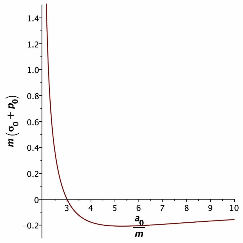
Figure 1: The graph shows $m\left(\sigma_{0}+p_{0}\right)$ versus $a_{0}/m$ for a symmetric Schwarzschild TSW. At $a_{0}=3m$, $m\left(\sigma_{0}+p_{0}\right)=0$ which confirms the previous results. Note that while $\sigma_{0}+p_{0}$ is positive valued pre-$3m$, it is negative post-$3m$. This explaines $\lim_{a_{0}\rightarrow 3m^{\pm}}\beta_{0}^{2}=\mp\infty$ in the original stability diagram.

The Extremal Reissner-Nordström TSW)

The case of an extremal Reissner-Nordström (ERN) TSW has also been considered in the literature Eiroa2 ; Sharif3 ; Mazhari1 . Having

$$\left\{\begin{array}[]{c}f_{\pm}=\left(1-\frac{m_{\pm}}{r_{\pm}}\right)^{2}\\ h_{\pm}=r_{\pm}^{2}\end{array}\right.,$$ (18)

as the metric function of ERN, we obtain

$$\sigma_{0}+p_{0}=-\frac{2\left[a_{0}-\left(\epsilon+2\right)m\right]}{a_{0}^{2}}.$$ (19)

Accordingly, there must be an infinite discontinuity at

$$a_{\text{ID}}=\left(\epsilon+2\right)m.$$ (20)

As shown in Eiroa2 , this also admits an infinite discontinuity at $a_{0}=2m$ for a symmetric ERN TSW, when $\epsilon=0$. For such a symmetric TSW, analogous to the previous case, $\lim_{a_{0}\rightarrow 2m^{\pm}}\beta_{0}^{2}=\mp\infty$, according to Fig. 2 plotted for $m\left(\sigma_{0}+p_{0}\right)$ versus $a_{0}/m$.

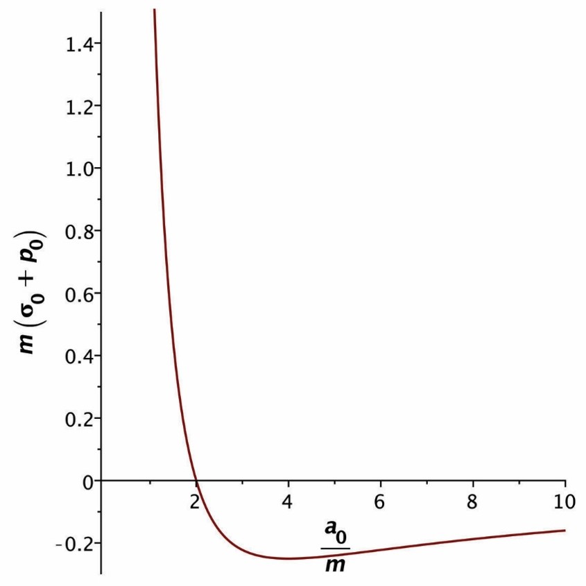
Figure 2: The graph of $m\left(\sigma_{0}+p_{0}\right)$ against $a_{0}/m$ for a symmetric ERN TSW. The zero of the vertical axis at $a_{0}=2m$ is expected according to the previous studies.

The Dilaton TSW)

In Eiroa1 , Eiroa studies a TSW constructed by two symmetric spacetimes which are solutions of the action

$$S=\int d^{4}x\sqrt{-g}\left[-R+\left(\nabla\phi\right)^{2}+e^{-2b\phi}F^{2}\right].$$ (21)

Herein, $g=\det\left(g_{\mu\nu}\right)$, $R$ is the Ricci scalar, $\phi$ is the scalar dilaton field, $F=F^{\mu\nu}F_{\mu\nu}$ with $F_{\mu\nu}$ being the electromagnetic field, and $b\in\left[0,1\right]$ is the coupling parameter between the dilaton and the electromagnetic field. In Schwarzschild coordinate the spherically symmetric solution is given by

$$ds^{2}=-f\left(r\right)dt^{2}+f^{-1}\left(r\right)dr^{2}+h\left(r\right)d\Omega^{2}$$ (22)

where the metric functions are Garfinkle1 ; Gibbons1

$$\left\{\begin{array}[]{c}f\left(r\right)=\left(1-\frac{A}{r}\right)\left(1-\frac{B}{r}\right)^{\left(1-b^{2}\right)/\left(1+b^{2}\right)}\\ h\left(r\right)=r^{2}\left(1-\frac{B}{r}\right)^{2b^{2}/\left(1+b^{2}\right)}\end{array}\right..$$ (23)

The constants $A$ and $B$ are related with the mass $m$ and charge $q$ of the spacetime through

$$\left\{\begin{array}[]{c}A=m\pm\sqrt{m^{2}-\left(1-b^{2}\right)q^{2}}\\ B=\left(1+b^{2}\right)q^{2}/A\end{array}\right..$$ (24)

Here we consider only the plus sign, for it is the plus sign that corresponds to the Schwarzschild metric when $q=0$. The solutions for $b=0$ reduce to the normal RN solutions for the Einstein-Maxwell action with a scalar field. For $b=1$ a family of static, spherically symmetric charged solutions in the context of low-energy string theory are recovered Garfinkle1 . Moreover, for $0\leq q^{2}<1+b^{2}$ the solution is a black hole with an event horizon at $r=A$ and an inner horizon at $r=B$. When $1+b^{2}\leq q^{2}\leq 1/\left(1-b^{2}\right)$, the inner horizon grows larger than the event horizon and the metric exhibits a naked singularity. Also, the spacetime is not well-defined if $q^{2}>1/\left(1-b^{2}\right)$. In what follows $a_{0}$ is considered to be greater than $A$ and $B$, as it must be.

According to the solution in Eqs. (22) and (23), it is expected that the root of the denominator in the expression for $\beta_{0}^{2}$ in Eq. (13) denotes the infinite discontinuity in the stability diagram. Having considered, the static energy density as

$$\sigma_{0}=-2\frac{h_{0}^{\prime}}{h_{0}}\sqrt{f_{0}},$$ (25)

and the static pressure as

$$p_{0}=\left(\frac{f_{0}^{\prime}}{f_{0}}+\frac{h_{0}^{\prime}}{h_{0}}\right)\sqrt{f_{0}},$$ (26)

one calculates for the roots of the denominator of $\beta_{0}^{2}$ in Eq. (13), to acquire $a_{\text{ID}}$. Due to the relatively complicated forms of $f\left(r\right)$ and $h\left(r\right)$ in Eq. (23), the expression for $a_{\text{ID}}$ is complicated and lengthy, too. For this reason, we refrain from bringing its explicit form here. Instead, we summarize the results in Fig. 3. Considering five different values for $b$, the subfigures display $a_{\text{ID}}$, the event horizon ($EH$) associated with $r=A$, and the inner horizon ($IH$) associated with $r=B$, in diagrams of $a_{\text{ID}}/m$ against $\left|q\right|/m$. The results are in complete agreement with the ones in Eiroa1 . For instance, for $b=0$ in Fig. 3a, there always exists an infinite discontinuity beyond horizons. As numerical examples, this discontinuity is $a_{\text{ID}_{+}}=3m$ for $\left|q\right|/m=0$, and $a_{\text{ID}_{+}}\simeq 2.485m$ for $\left|q\right|/m=0.8$, as expected. Note that $\left|q\right|/m>1$ is not permitted due to the restricting conditions on the bulk spacetime mentioned above. In the case $b=1$, on the other hand, for $\left|q\right|/m\geq\sqrt{2}$ there is no infinite discontinuity. Again, for the sake of comparison to the results in Eiroa1 , note that, for example, when $\left|q\right|/m=0.8$ we obtain $a_{\text{ID}}\simeq 2.594m$, and $a_{\text{ID}}\simeq 2.860m$, when $b=0.5$, and $b=1$, respectively. Furthermore, remark that $a_{\text{ID}}$ in all cases is $3m$ when $\left|q\right|/m=0$, for the simple fact that when $q=0$, the metric functions in Eq. (23) reduce to the Schwarzschild metric functions, regardless of the value of $b$.

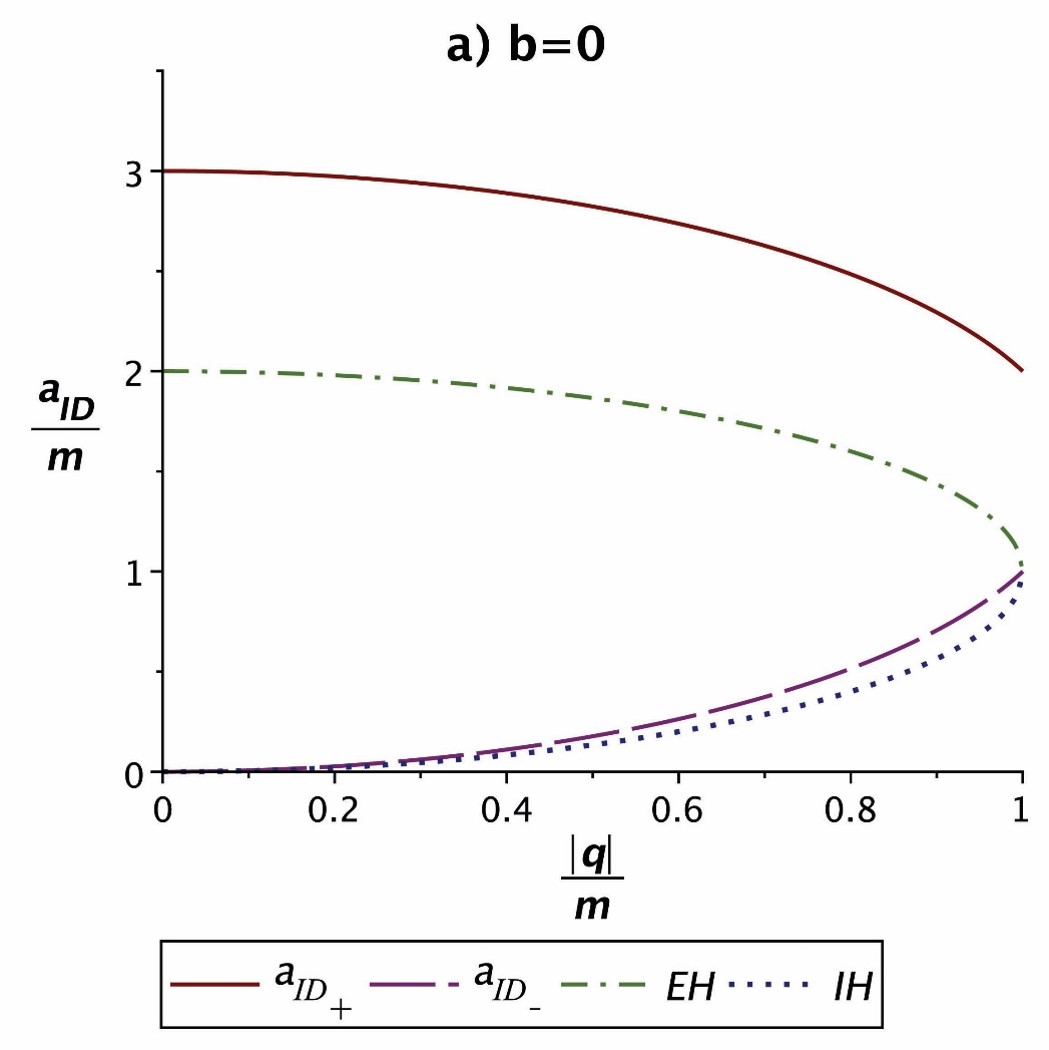
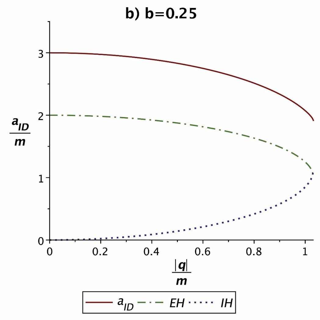
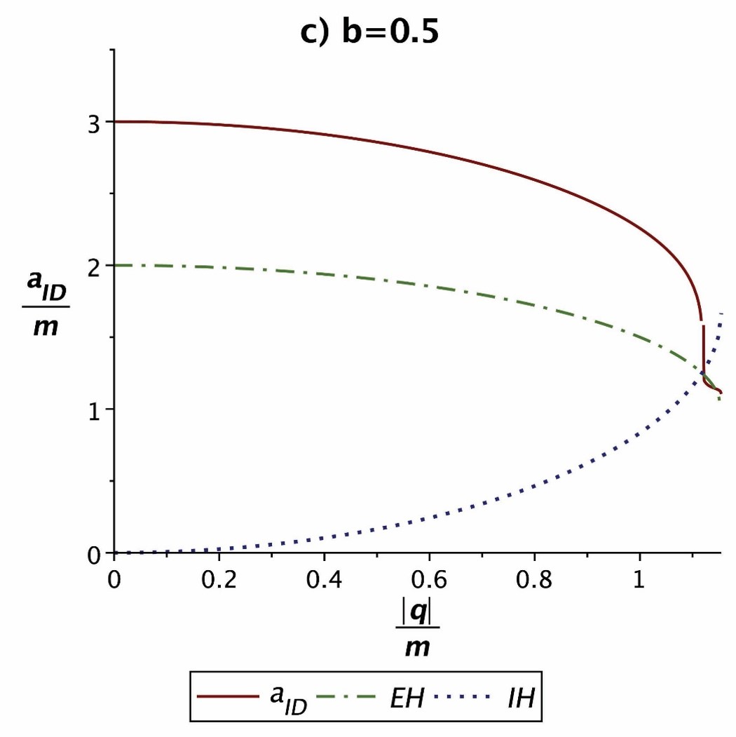
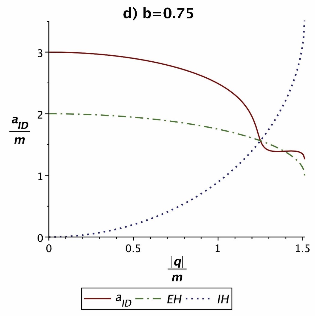
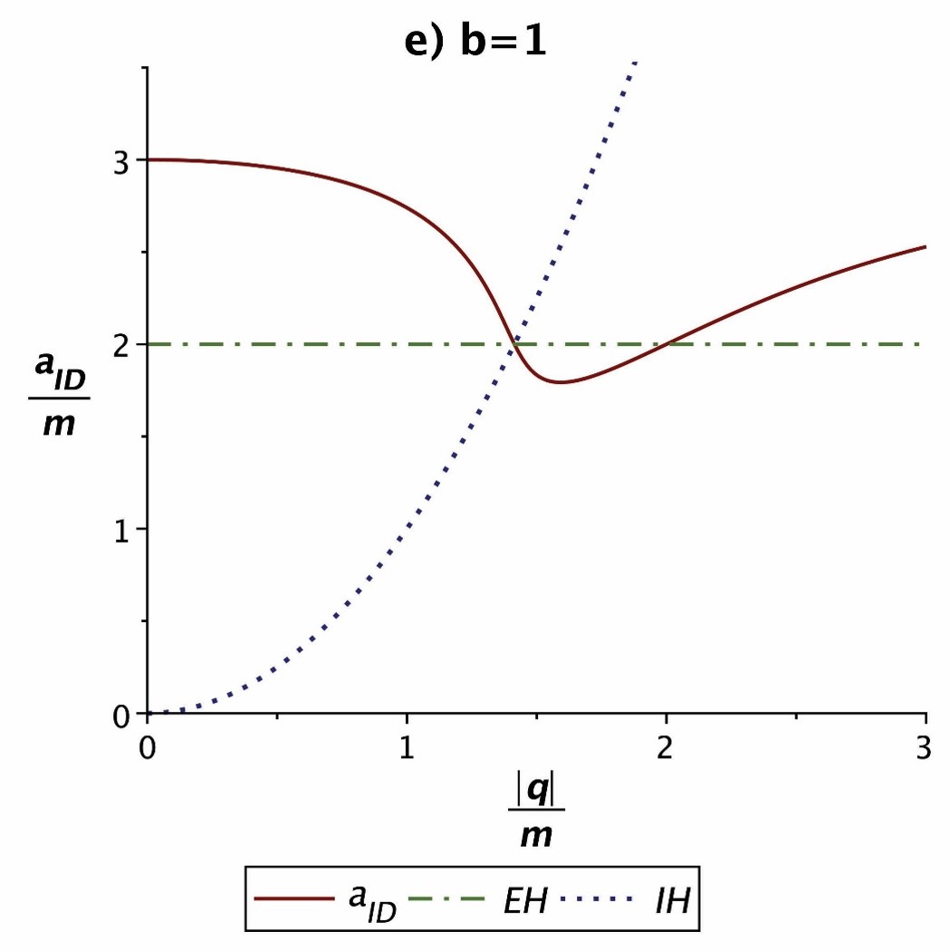
Figure 3: The graphs show $a_{\text{ID}}/m$ against $|q|/m$ for a dilaton TSW for different values of $b$. In the legend, $a_{\text{ID}_{+}}$ and $a_{\text{ID}_{-}}$ correspond to the roots of the denominator of $\beta_{0}^{2}$, given in Eq. (30). Also, $EH$ and $IH$ correspond to the event horizon and the inner horizon of the bulk universe.

IV Variable EoS

In 2015, Varela demonstrated that the infinite discontinuity of a Schwarzschild TSW can be removed by using a rather different EoS called the variable EoS Varela1 . Mathematically shown as $p=p\left(\sigma,a\right)$, the variable EoS grants the pressure an explicit radius-dependency. As a consequence, Eq. (11) will be replaced by

$$p_{0}^{\prime}=\beta_{0}^{2}\sigma_{0}^{\prime}-\gamma_{0},$$ (27)

where now $\gamma_{0}\equiv-\left.\partial p/\partial a\right|_{a_{0}}$. The mechanism of infinite discontinuity removal by the variable EoS is simply to make null the numerator of

$$\beta_{0}^{2}=\frac{p_{0}^{\prime}+\gamma_{0}}{-\frac{h_{0}^{\prime}}{h_{0}}\left(\sigma_{0}+p_{0}\right)+\frac{2h_{0}h_{0}^{\prime\prime}-h_{0}^{\prime 2}}{2h_{0}h_{0}^{\prime}}\sigma_{0}}$$ (28)

at $a_{\text{ID}}$, where the discontinuity used to happen when $\gamma_{0}$ was zero. This means, if we set $\gamma_{0}$ such that

$$\gamma_{0}=-p_{0}^{\prime},$$ (29)

then $\lim_{a_{0}\rightarrow a_{\text{ID}}}\beta_{0}^{2}=\frac{0}{0}$ is indefinite, and it becomes well-defined if the numerator approaches zero, at least, at the same rate as the denominator. As far as the unit convention that is applied here concerns, $\beta_{0}^{2}$ is a dimensionless quantity ($\beta_{0}$ is of type speed, with the SI dimension $\left[LT^{-1}\right]$, which becomes dimensionless here, since length and time are looked at on an equal footing in general relativity). Hereupon, the numerator and the denominator of $\beta_{0}^{2}$ have the same dimension ($L^{-2}$), and in case the fine-tuning $\gamma_{0}=-p_{0}^{\prime}$ is exerted, $\beta_{0}^{2}$ can be well-defined. Note that Eq. (28) is somehow a generalization to Eq. (13).

For the case of a symmetric Schwarzschild TSW one obtains

$$\left.p_{0}^{\prime}\right|_{a_{0}=3m}=-\frac{2\sqrt{3}}{9m^{2}},$$ (30)

by taking the first derivative of Eq. (6), applying Eq. (15) and setting $\epsilon=0$. This means that by fine-tuning $\gamma_{0}$ to $2\sqrt{3}/\left(9m^{2}\right)$ we may be free of infinite discontinuity in the stability diagram. This is particularly shown in Fig. 4 for $\beta_{0}^{2}$ against $a_{0}/m$. As it is evident, there is no sign of the infinite discontinuity anymore.

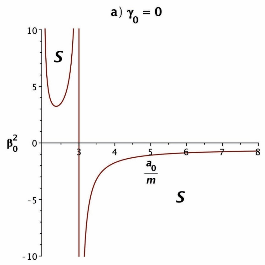
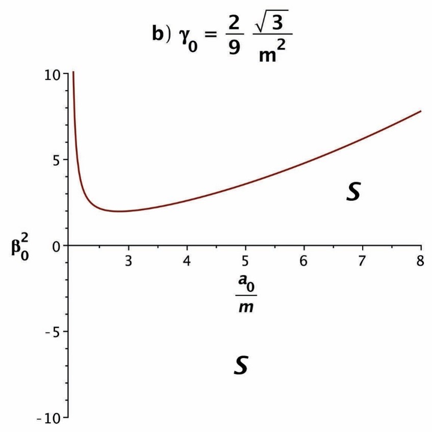
Figure 4: The stability diagram for a symmetric Schwarzschild TSW with $a)$ the barotropic EoS and $b)$ the variable EoS. It can be observed that the infinite discontinuity is simply removed by virtue of the variable EoS.

Applying the variable EoS to an ERN ATSW leads to the same result. In this case we obtain

$$\left.p_{0}^{\prime}\right|_{a_{0}=\left(\epsilon+2\right)m}=-\frac{2}{\left(\epsilon+2\right)^{2}m^{2}},$$ (31)

as the derivative of the angular pressure at the radius of infinite discontinuity occurrence. Correspondingly, the choice $\gamma_{0}=2/\left(\left(\epsilon+2\right)^{2}m^{2}\right)$ is expected to remove the infinite discontinuity. Fig. 5 shows how this happens for a symmetric ERN TSW, for which $\epsilon=0$.

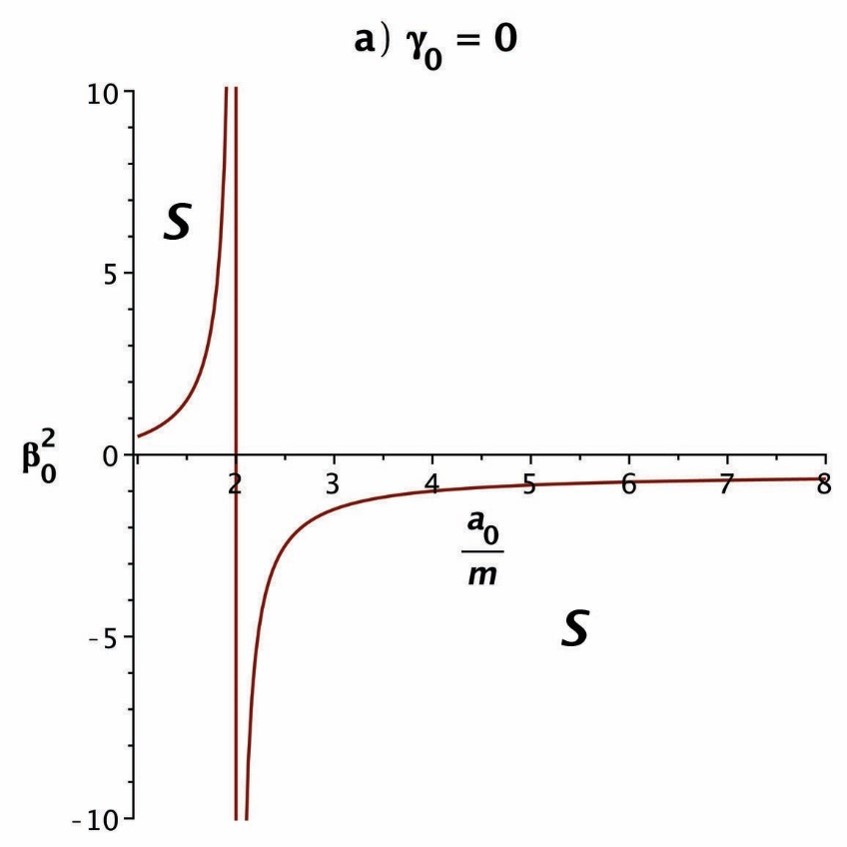
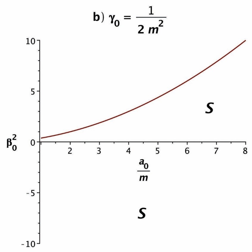
Figure 5: The stability diagram for a symmetric ERN TSW with $a)$ the barotropic EoS and $b)$ the variable EoS. As expected, the infinite discontinuity is removed due to the fine-tunning of the variable EoS.

In the end, we turn our attention to the dilaton TSW. Here we will have a closer look at three cases for which $b=0$, $b=0.5$, and $b=1$. The former is selected for it defines the RN spacetime, and the latter is selected for its importance in string theory. The choice $b=0.5$ is rather random, as a middling value in the $b$-spectrum. Also, for all three cases, without loss of generality, we have randomly chosen $\left|q\right|/m=0.5$. Our numerical analysis shows that for the three case we have

$$\left\{\begin{array}[]{c}\left.p_{0}^{\prime}\right|_{a_{0}=a_{\text{ID}}}\simeq-0.4139864432/m^{2}\text{ \ \ when \ \ }b=0\\ \left.p_{0}^{\prime}\right|_{a_{0}=a_{\text{ID}}}\simeq-0.4146553639/m^{2}\text{ \ \ when \ \ }b=0.5\\ \left.p_{0}^{\prime}\right|_{a_{0}=a_{\text{ID}}}\simeq-0.4162095590/m^{2}\text{ \ \ when \ \ }b=1\end{array}\right.,$$ (32)

which denotes that if we fine-tune $\gamma_{0}$ such that $\left.\gamma_{0}\right|_{b=0}=0.4139864432/m^{2}$, $\left.\gamma_{0}\right|_{b=0.5}=0.4146553639/m^{2}$, and $\left.\gamma_{0}\right|_{b=1}=0.4162095590/m^{2}$, the existed discontinuities must be removed. This can be seen clearly in Fig. 6, where the related mechanical stability diagrams are plotted for the three cases, once when $\gamma_{0}=0$ (barotropic EoS), and once when it is fine-tuned to remove the discontinuity. In all the subfigures, the horizontal axis starts at $A/m$, and the stable regions are marked with an “S”. Note that a similar analysis can be applied to other admissible values of $b$ and/or $\left|q\right|/m$.

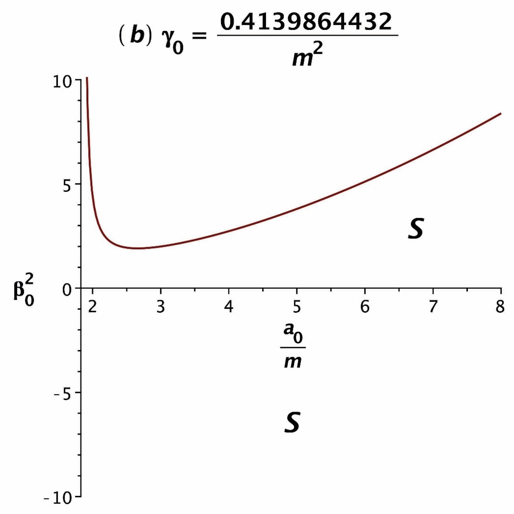
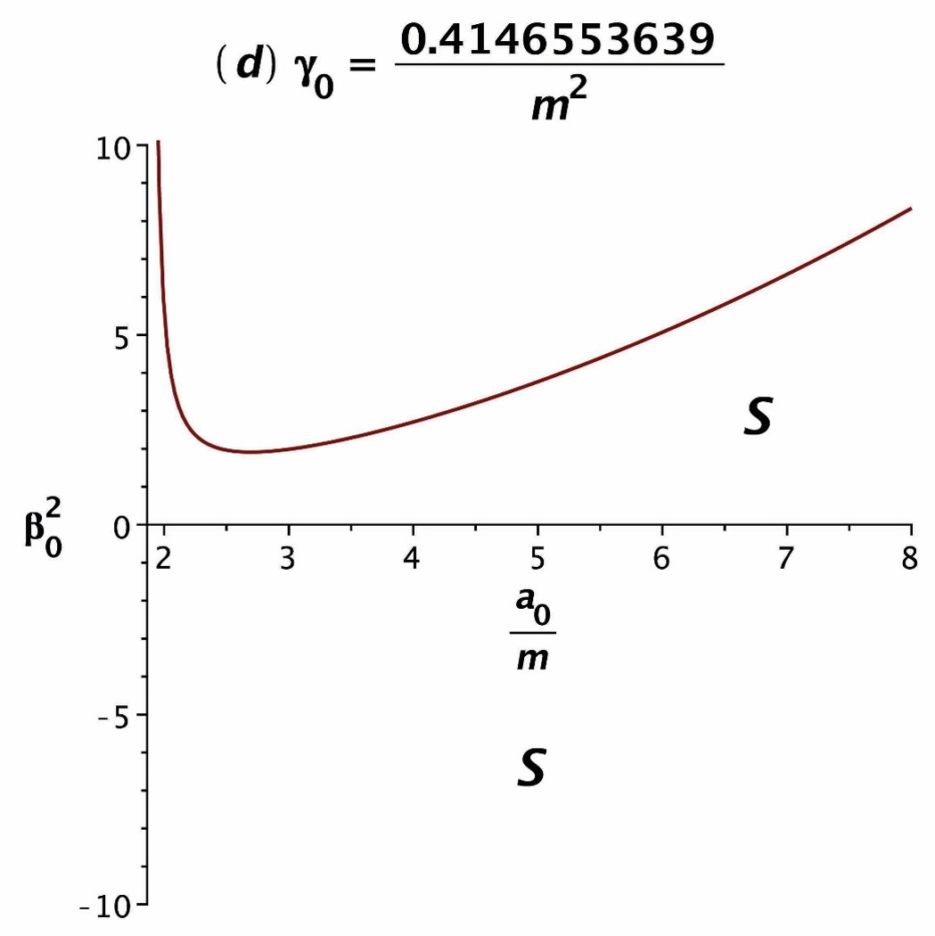
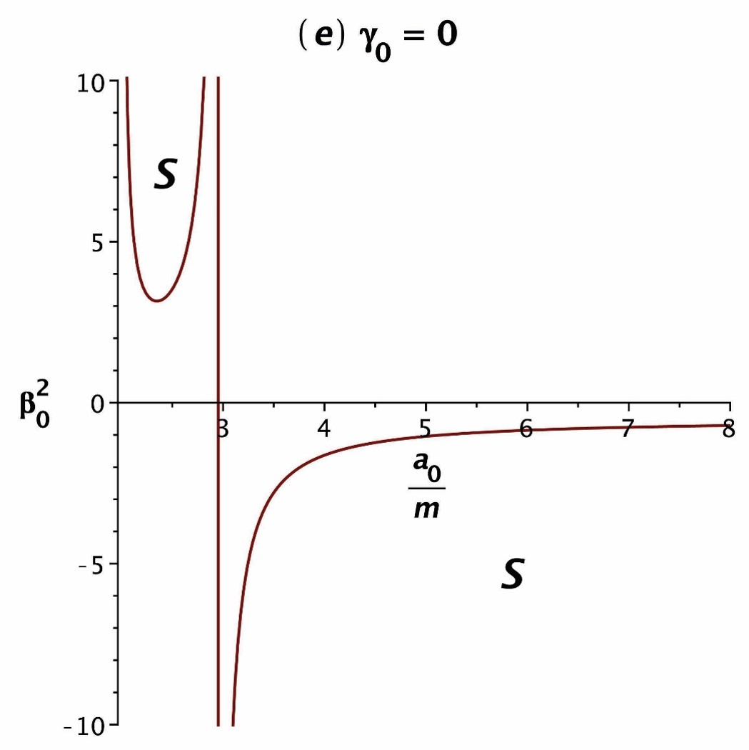
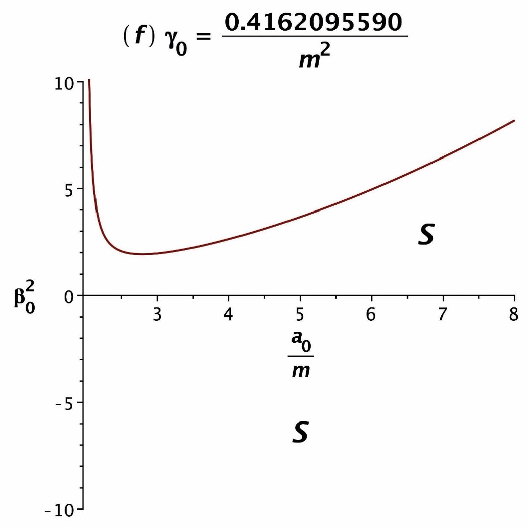
Figure 6: The stability diagram for a symmetric dilaton TSW for $a)$ $b=0$ with a barotropic EoS, $b)$ $b=0$ with a fine-tuned variable EoS, $c)$ $b=0.5$ with a barotropic EoS, $d)$ $b=0.5$ with a fine-tuned variable EoS, $e)$ $b=1$ with a barotropic EoS, and $f)$ $b=1$ with a fine-tuned variable EoS. The value of $\left|q\right|/m$ is set half for all the cases. The fine-tuned values of $\gamma_{0}$ are given at the top of each diagram. The regions with “S” are where the TSW is mechanically stable.

V Conclusion

The emergence of infinitely branching discontinuity, resembling a phase transition, seemed peculiar enough to attract attention since the stability analyses for TSWs were incepted. The prototype example was the Schwarzschild TSW which had such a discontinuity at the stability radius $a_{0}=3m$, as pointed out by Poisson and Visser Poisson1 . In analogy, other TSWs also exhibited similar behavior. We identified the cause of such type of discontinuities: they arise from the vanishing of $-\left(h_{0}^{\prime}/h_{0}\right)\left(\sigma_{0}+p_{0}\right)+\left(2h_{0}h_{0}^{\prime\prime}-h_{0}^{\prime 2}\right)\sigma_{0}/2h_{0}h_{0}^{\prime}$ at equilibrium radius (Eq. (13)). In consequence, the speed of sound $\beta_{0}$, which is inversely proportional to this expression, and is expected to be finite, naturally diverges. In an attempt to resolve such a discontinuity in the symmetric Schwarzschild TSW, Varela employs a more general, modified EoS, i.e. the variable EoS, to replace the barotropic one. In this rather general EoS, the pressure $p$ depends, beside $\sigma$, also on the radius of the shell which creates an extra degree of freedom to be used as an advantage. We have precisely shown that such a generalization can be systematically applied to all the TSWs, by pointing out to the reason of the emergence of the discontinuities. Our investigation is generalized to all spherically symmetric spacetimes, with the generic line element in Eq. (1), including non-asymptotically flat ones such as the dilaton TSW in section $IIIc$. This shows that the method is applicable even to those TSWs which are strongly coupled with the non-linear, non-asymptotically flat, dilatonic bulk spacetimes. In section $IV$, the logic was illustrated by representing three examples (see Fig. 4 for the Schwarzschild, Fig. 5 for ERN TSWs and Fig. 6 for the dilaton TSW), where as a result, the discontinuities in question are eliminated. It is not difficult to anticipate that the same technique can be applied also to other TSWs, including the ones in alternative theories. Finally, let us add that in the present article, we used asymmetric TSW in the sense that the spacetimes on different sides of the throat differ only parametrically. No doubt, the spacetimes that differ in $r$-dependence also can be considered within the range of application.

References

- (1) M. Visser, Phys. Rev. D 39, 3182 (1989).
- (2) M. Visser, Nucl. Phys. B 328, 203 (1989).
- (3) M. Azreg-Aïnou, J. Cosmol. Astropart. Phys. 07, 037 (2015).
- (4) N. M. Garcia, F. S. N. Lobo and M. Visser, Phys. Rev. D 86, 044026 (2012).
- (5) V. Varela, Phys. Rev. D 92, 044002 (2015).
- (6) M. G. Richarte, I. G. Salako, J. P. Morais Graca et al., Phys. Rev. D 96, 084022 (2017).
- (7) M. Sharif and Z. Yousaf, Astrophys. Space Sci 351, 351 (2014).
- (8) M. Sharif and M. Azam, Eur. Phys. J. C 73, 2407 (2013).
- (9) N. Montelongo Garcia, F. S. N. Lobo and M. Visser, Phys. Rev. D 86, 044026 (2012).
- (10) G. A. S. Dias and J. P. S. Lemos, Phys. Rev. D 82, 084023 (2010).
- (11) E. F. Eiroa, Phys. Rev. D 78, 024018 (2008).
- (12) M. Thibeault, C. Simeone and E. F. Eiroa, Gen. Relativ. Gravit. 38, 1593 (2006).
- (13) F. S. N. Lobo and P. Crawford, Class. Quantum Grav. 21, 391 (2004).
- (14) E. F. Eiroa and G. E. Romero, Gen. Rel. Gravit. 36, 651 (2004).
- (15) E. F. Eiroa and C. Simeone, Phys. Rev. D 70, 044008 (2004).
- (16) M. Ishak and K. Lake, Phys. Rev. D 65, 044011 (2002).
- (17) M. Visser, Lorentzian Wormholes: From Einstein to Hawking (American Institute of Physics, New York, 1995).
- (18) M. S. Morris and K. S. Thorne, Am. J. Phys. 56, 395 (1988).
- (19) S. D. Forghani, S. H. Mazharimousavi and M. Halilsoy, Eur. Phys. J. C 78, 469 (2018).
- (20) S. D. Forghani, S. H. Mazharimousavi and M. Halilsoy, arXiv:1807.05080 (2018).
- (21) S. D. Forghani, S. H. Mazharimousavi and M. Halilsoy, Eur. Phys. J. Plus 133, 497 (2018).
- (22) E. Poisson and M. Visser, Phys. Rev. D 52, 7318 (1995).
- (23) W. Israel, Nuovo Cimento 44B, 1 (1966).
- (24) M. C. Bento, O. Bertolami and A. A. Sen, Phys. Rev. D 66, 043507 (2002).
- (25) A. Eid, Astrophys. Space Sci. 364, 8 (2019).
- (26) M. Sharif and M. Azam, Eur. Phys. J. C 73, 2554 (2013).
- (27) S. Habib Mazharimousavi and M. Halilsoy, Int. J. Mod. Phys. D 27, 1850028 (2018).
- (28) D. Garfinkle, G. T. Horowitz and A. Strominger, Phys. Rev. D 43, 3140 (1992); Erratum Phys. Rev. D 45, 3888 (1992).
- (29) G. W. Gibbons and K. Maeda, Nucl. Phys. B 298, 741 (1988).