A robust anomaly finder based on autoencoders

Abstract

We propose a robust method to identify anomalous jets by vetoing QCD-jets. The robustness of this method ensures that the distribution of the proposed discriminating variable (which allows us to veto QCD-jets) remains unaffected by the phase space of QCD-jets, even if they were different from the region on which the model was trained. This suggests that our method can be used to look for anomalous jets in high $m/p_{T}$ bins by simply training on jets from low $m/p_{T}$ bins, where sufficient background-enriched data is available. The robustness follows from combining an autoencoder with a novel way of pre-processing jets. We use momentum rescaling followed by a Lorentz boost to find the frame of reference where any given jet is characterized by predetermined mass and energy. In this frame we generate jet images by constructing a set of orthonormal basis vectors using the Gram-Schmidt method to span the plane transverse to the jet axis. Due to our preprocessing, the autoencoder loss function does not depend on the initial jet mass, momentum or orientation while still offering remarkable performance. We also explore the application of this loss function combined (using supervised learning techniques like boosted decision trees) with few other jet observables like the mass and Nsubjettiness for the purpose of top tagging. This exercise shows that our method performs almost as well as existing top taggers which use a large amount of physics information associated with top decays while also reinforcing the fact that the loss function is mostly independent of the additional jet observables.

1 Introduction

With the recent discovery of the $125~{}\text{GeV}$ Higgs by CMS Chatrchyan:2012xdj and ATLAS Aad:2012tfa collaborations of the LHC, the last missing link in the standard model (SM) of particle physics is completed. The focus has now shifted to find physics beyond the standard model (BSM), for which there are plethora of candidates all designed to solve various short comings of SM. Unfortunately, we have failed to observe any trace of physics beyond the standard model (BSM) so far in all our searches for these “well-motivated” scenarios. At this juncture, it may well be equally justifiable to concentrate on the “Bottom-up” approach of looking for the “unexpected” in data, apart from the usual “Top-down” approach of first hypothesizing an extension to the SM and then predicting its phenomenology. Even though this “Bottom-up” approach is nothing other than looking for deviations from the SM background and there has been remarkable progress recently in automated precision (higher order) calculations (radiative corrections due to quantum chromodynamics (QCD) and electroweak (EW) interactions as well), it is still extremely difficult (impractical) to precisely estimate all backgrounds due to SM without using data. In this context, searching for new physics (NP) as anomalies directly from data depict a qualitatively new and highly promising direction.

Note that the philosophy of hunting for NP as anomalies where data is used to estimate background is already a common practice in jet physics. A simple example is the search for boosted massive resonances using jet-mass $m_{J}$. The background is generically due to QCD-jets. The well-studied and well-understood variable $\frac{d{\sigma}}{d{m_{J}}}$ for QCD-jets has a continuously falling distribution at high $m_{J}$. Any massive resonance decaying hadronically and boosted enough such that all its decay products is contained in a jet, shows up as a bump peaked around its mass. Looking for these bumps over a falling spectrum provides one such simplistic example where one does not need to rely on the exact nature of the massive resonance (as long as it decays hadronically). Knowing this falling distribution due to QCD is enough, in principle, to look for unknown new particles. Additionally, jet masses for boosted massive resonances are robust under various jet grooming procedures Butterworth:2008iy ; Salam:2009jx ; Krohn:2009th ; Ellis:2009me , owing to their substructures, as compared to jet masses for QCD-jets. Searching for bumps in the distribution for groomed jet masses, therefore, provides a model-independent way to look for hadronically decaying NP particles with substantial discovery potential. One can even take, massive resonances of SM like the $W^{\pm},Z$ gauge bosons, Higgs particle $h$, and top quark $t$, as test cases to hone this search procedure. A broader generalization of this philosophy, is given in Ref Chakraborty:2017mbz , where the authors use a large set of jet-shape observables to construct a veto for standard objects such as QCD-jets, photons, leptons, etc. Jets that pass this veto, would be termed anomalies. Examples of such anomalies include jets containing decay products (not restricted to hadrons only) of NP resonances, long-lived particles etc.

Machine learning can be of a big help in looking for such anomalies by constructing an anti-QCD tagger Aguilar-Saavedra:2017rzt . The traditional applications Cohen:2017exh ; Qu:2019gqs ; Datta:2017rhs ; Moore:2018lsr ; Komiske:2018cqr ; Butter:2017cot ; Komiske:2017aww ; Louppe:2017ipp ; Erdmann:2018shi ; Hocker:2007ht ; Pearkes:2017hku ; Almeida:2015jua ; Macaluso:2018tck ; Kasieczka:2017nvn ; Cogan:2014oua ; Baldi:2016fql ; deOliveira:2015xxd ; Collins:2019jip ; Kasieczka:2019dbj ; Collins:2018epr of machine learning techniques for classification problems in collider physics are, however, centered around the idea of supervised learning where the training data is labeled into various categories and the model tries to correctly classify the training data into these categories. However, this method is inadequate when a model needs to be trained directly on data which is not labeled. This is where autoencoders, which are unsupervised learning algorithms Cerri:2018anq ; Andreassen:2018apy ; Farina:2018fyg ; Heimel:2018mkt ; Hajer:2018kqm , can be useful. Because of training, an autoencoder learns to reproduce QCD-jets efficiently, and it is expected to be not as effective at reproducing jets originating from other processes, resulting in larger “loss-functions”. Therefore, the loss function of the autoencoder can be used to find anomalies Farina:2018fyg ; Heimel:2018mkt ).

An essential requirement for a high performance machine learning based anomaly finder, is that it needs to be trained with control samples of QCD-jets. Since one expects anomalies to appear within samples of jets at high jet masses, one essentially needs to train using QCD-jets of high masses. Note however, as pointed out in Ref. Dasgupta:2013ihk , a better variable to understand the underlying physics of QCD-jets is the dimensionless variable $\rho\equiv\frac{m_{J}}{p_{T}R}$, where $R$ reflects the size of jets. The issue of training with large jet masses, therefore, gets translated to training using jets with a large $\rho$ (given that jets are constructed using a minimum $p_{T}$ and an $R$-parameter). In any case, it is difficult to obtain sufficiently pure samples of QCD-jets with high jet-mass or a high $\rho$ from data itself. Apart from contamination effects, it is also difficult to gather sufficient training data in these high mass bins. This problem can be partially mitigated if one can use trainings on jets from low $\rho$ bins, which are relatively more pure in QCD-jets and at the same time are easily available. In order to implement this strategy, however, we require an anomaly hunter that is robust. Technically speaking, by robustness we here refer to the criteria that the distribution of the loss-function for QCD-jets remains unaltered even if training samples from different $\rho$ bins are used.

Unfortunately, when an autoencoder is trained in a naive way, it tends to learn features which have large correlations with the jet mass. This is expected since the jet mass is a powerful observable to characterize a jet. Therefore, generically speaking, one does not expect a simple autoencoder based anomaly hunter or anti-QCD tagger to be robust. It is not a surprise that previous attempts in this direction Farina:2018fyg ; Heimel:2018mkt find significant dependence of autoencoder loss on jet masses. Consequently, cuts on such jet mass dependent loss functions necessarily sculpt the jet mass distribution itself, which makes techniques like bump hunts (for boosted massive resonances) and side band analyses much more challenging. Ref. Farina:2018fyg suggests using convolution autoencoders, since these are less affected by the above problem. However, the improvement in robustness is marginalFarina:2018fyg . On the other hand, Ref. Heimel:2018mkt tries to alleviate this problem using adversary training to reduce the dependence of jet mass on autoencoder response. This technique requires an additional network to try and guess the mass from the output of the first network, which is added complexity requiring significantly larger computation to train the network and leads to decrease in transparency. Also, it is not a general purpose method in that it is not applicable for autoencoders based on Lorentz layers Heimel:2018mkt .

In this work, we present a robust anti-QCD tagger based on autoencoders. The robustness comes due to a series of novel preprocessing stages, and therefore can be easily generalized for many other cases such as an autoencoder based on the Lorentz layer or even supervised learning problems. Summarizing, the method proceeds as follows:

• Given a jet, the algorithm first rescales and then boosts to a frame of reference where the mass and energy of the jet gets fixed to predetermined values (denoted here by $m_{0}$ and $E_{0}$ respectively).

• The Histogram, representing the jet image is filled by using the dimensionless number $E_{i}/E_{0}$, where $E_{i}$ represents the energy of each constituent in this new frame. Also, in order to remove residual rotational symmetries present in the plane transverse to the jet-axis, the transverse plane is spanned using an orthonormal set of basis vectors, constructed using Gram-Schmidt procedure on either two hardest subjets, or two hardest constituents.

We find that this method has a remarkable effect that it makes QCD-jets in different $\rho$ bins to appear similar as viewed by the network. As a result, an autoencoder trained on jet data in the lower $\rho$ bins (where data is surplus and pure) can be used in searches for anomalies in a set of jets at the higher $\rho$ bins (where data is scarce and may be contaminated). Computationally, it is a far simpler and cheaper solution for removing the dependence of autoencoder loss on the jet mass compared to the proposal in Ref. Heimel:2018mkt . At the same time, this method yields significantly more robust performance than Ref. Farina:2018fyg . These highly desirable characteristics in this proposal make it highly portable and easily usable in many important techniques like mass bump hunt and side band analyses at all energy scales.

We also take this opportunity to study the performance of fully-connected and convolution autoencoders as anomaly finders, where the jets are preprocessed using the methods proposed here. In order to benchmark, we treat top-jets and $W$-jets as anomalies. Here top-jets and $W$-jets refer to jets containing decay products of hadronically decaying boosted top and $W$ respectively. We find that our anomaly finder, trained on only QCD-jets, yields performance comparable to Ref. Farina:2018fyg . On the other hand, when combined with the mass of jets, it tags top as efficiently as HEPTopTagger2 Plehn:2011tg ; Kasieczka:2015jma ; Plehn:2010st ; Plehn:2009rk , which uses a large amount of physics information specific to top decays. Additionally, when combined with Nsubjettiness, it substantially outperforms HEPTopTagger2 Plehn:2011tg ; Kasieczka:2015jma ; Plehn:2010st ; Plehn:2009rk . Summarizing, we propose a new anomaly finder that yields remarkable robustness without sacrificing performance. Additionally, we also benchmark the effectiveness of the anomaly finder when jets consisting of all decay products of a boosted NP particle decaying to $W^{+}W^{-}$, each of which in turn, decay hadronically, is treated as an anomalous jet. Being remarkably robust to giving high discovery potentials for finding anomalous jets, we find our method to generate impressive performances.

The rest of this document is organized as follows: in Sec. 2, we describe in detail our method of preprocessing, and give a brief description of the autoencoder we use for this study; in Sec. 3, we present main results of this study after specifying all simulation details; and finally we conclude in Sec. 4.

2 Our Proposed Analysis

Our method can be broadly divided into two main parts. In the first part, we take jets from the event as input and produce images corresponding to these jets as described in Subsec. 2.1. The second part of our method involves the autoencoder. In Subsec. 2.2, we describe the general features of the autoencoder and explain how it can be trained.

2.1 From an infrared safe jet to the jet image

Our method requires jets as inputs. A jet is basically a collection of four momenta of its constituents which are clustered according to any of the infrared-safe or IR-safe Sterman:2008kj sequential jet clustering algorithm like Anti-$k_{t}$ Cacciari:2008gp , Cambridge/Aachen (C/A) Dokshitzer:1997in and $k_{t}$ Ellis:1993tq ; Catani:1993hr or IR-safe cone based algorithms (like SISCone) Blazey:2000qt ; Salam:2009jx . In this work, we use the notation $P_{J}^{\mu}$ ($\vec{P}_{J}$) for the four-momentum (three-momentum) of the jet, $p_{i}^{\mu}$ ($\vec{p}_{i}$) for the four-momentum (three-momentum) of the $i^{\text{th}}$ constituent in the jet. We use “E-scheme” Cacciari2012 , where the four-momenta of the jet is simply the vector sum of four-momenta of its constituents.

$$P_{J}^{\mu}\ =\ \sum_{i=1}^{N_{J}}p_{i}^{\mu}\;,\quad{m_{J}}^{2}\ \equiv\ \left|P_{J}^{\mu}\right|^{2}\ =\ \left(P^{0}_{J}\right)^{2}-\left(\vec{P_{J}}\right)^{2}\;,\text{ and}\quad E_{J}\ \equiv\ P_{J}^{0}\;,$$ (1)

where $N_{J}$ is the total number of constituents, $m_{J}$ the jet mass, and $E_{J}$ is the jet energy.

2.1.1 Rescale the jet

In the first step, all the jet constituent four-momenta are rescaled such that the new jet mass is given by a preassigned $m_{0}$:

$$p_{i}^{\mu}\quad\rightarrow\quad\ p_{i}^{\prime\mu}\ =\ \frac{m_{0}}{m_{J}}\times p_{i}^{\mu}\qquad\Rightarrow\qquad P_{J}^{\mu}\quad\rightarrow\quad\ P_{J}^{\prime\mu}\ =\ \frac{m_{0}}{m_{J}}P_{J}^{\mu}\;.$$ (2)

Note that the energy of the “rescaled jet” $P^{\prime\mu}_{J}$, is given by $E_{J}^{\prime}=E_{J}m_{0}/m_{J}$.

2.1.2 Lorentz boost the jet

The next step involves performing a Lorentz boost $\left({\Lambda}^{\mu}_{\ \nu}\right)$ to a frame such that, in the new frame, all jets have a given energy $E_{0}$. In other words, the rescaled jets $\left({P^{\prime\mu}_{J}}\right)$ are Lorentz transformed to boosted jets $\left({\mathbf{P}_{J}^{\mu}}\right)$ such that:

$$\begin{split}p_{i}^{\prime\mu}\quad\rightarrow\quad\ \mathbf{p}_{i}^{\mu}\ =\ \Lambda^{\mu}_{\ \nu}\>p_{i}^{\prime\nu}&\qquad\Rightarrow\qquad P_{J}^{\prime\mu}\quad\rightarrow\quad\mathbf{P}_{J}^{\mu}\ =\ \Lambda^{\mu}_{\ \nu}\>P_{J}^{\prime\nu}\\ &\text{such that: }\mathbf{E}_{J}\ \equiv\ \mathbf{P}_{J}^{0}\ =\ E_{0}\;.\end{split}$$ (3)

Since this is a critical step in our method, we present a simple derivation. We need to determine both the direction of the boost and the $\gamma$ factor required for the boost. Starting with the rescaled jet (with the given jet mass $m_{0}$ and energy $E^{\prime}_{J}$), we can split the situation into 2 cases:

1. ${E_{J}^{\prime}>E_{0}}$: the boost is along the three-momentum direction of the jet and

2. $E_{J}^{\prime}<E_{0}$: the boost is opposite to the three-momentum direction of the jet

In order to determine the ${\gamma}$ factor required for the boost consider the first case $E_{J}^{\prime}>E_{0}$, where impose the condition that the boosted energy must be $E_{0}$.

$$E_{0}\ =\ \gamma\>E_{J}^{\prime}-\beta\gamma\>\left|\vec{P}_{J}^{\prime}\right|\qquad\text{where:}\quad\beta^{2}\ =\ 1-\frac{1}{\gamma^{2}}\;.$$ (4)

This gives:

$$\left(\frac{m_{0}^{2}}{\left|\vec{P}_{J}^{\prime}\right|^{2}}\right)\gamma^{2}+\left(-\frac{2E_{J}^{\prime}E_{0}}{\left|\vec{P}_{J}^{\prime}\right|^{2}}\right)\gamma+\left(\frac{{E_{0}}^{2}}{\left|\vec{P}_{J}^{\prime}\right|^{2}}+1\right)\ =\ 0\;,$$ (5)

where, we have used $m_{0}^{2}=\left(E^{\prime}_{J}\right)^{2}-\left|\vec{P}_{J}^{\prime}\right|^{2}$. Solving this quadratic equation in Eq. (6) and picking the smaller solution (so that we do not boost past the rest frame of the jet), we get:

$$\gamma\ =\ \frac{1}{m_{0}^{2}}\ \left(E_{J}^{\prime}E_{0}-P_{0}\left|\vec{P}_{J}^{\prime}\right|\right)\;,$$ (6)

where $P_{0}^{2}=E_{0}^{2}-m_{0}^{2}$ is the magnitude of three-momentum of the jet in the boosted frame.

In case $E_{J}^{\prime}<E_{0}$, we get the exact same solution for $\gamma$ but with the boost direction being opposite to the jet momentum. After boosting, we now have a jet with four-momentum $\mathbf{P}_{J}^{\mu}$ such that $\mathbf{E}_{J}=E_{0}$ and $\left|\mathbf{P}_{J}^{\mu}\right|^{2}={m_{0}}^{2}$.

2.1.3 Forming the images

A jet image is basically just a 2 dimensional histogram of the energy (or $p_{T}$) of its constituents with respect to the plane transverse to the jet axis. We use the Gram-Schmidt procedure to determine the optimal set of basis vectors in the transverse plane while also removing the residual rotation symmetry still present in the constituents.

Denoting the set of all constituent momenta in the boosted frame $\left\{\mathbf{p}_{1}^{\mu},\mathbf{p}_{2}^{\mu},\dots,\mathbf{p}_{N}^{\mu}\right\}$ such that $\mathbf{p}_{1}^{0}\geq\mathbf{p}_{2}^{0}\geq\dots\geq\mathbf{p}_{N}^{0}$, we construct the new set of basis vectors $\left\{\hat{e}_{1},\hat{e}_{2},\hat{e}_{3}\right\}$ obtained by the Gram-Schmidt method:

$$\hat{e}_{1} \ \equiv\ \frac{\vec{\mathbf{P}}_{J}}{\left|{\vec{\mathbf{P}}_{J}}\right|}\;,$$ (7)

$$\hat{e}_{2} \ \equiv\ \frac{\vec{\mathbf{p}}_{1}-\left(\vec{\mathbf{p}}_{1}\cdot\hat{e}_{1}\right)\hat{e}_{1}}{\left|\vec{\mathbf{p}}_{1}-\left(\vec{\mathbf{p}}_{1}\cdot\hat{e}_{1}\right)\hat{e}_{1}\right|}\;,$$ (8)

$$\hat{e}_{3} \ \equiv\ \frac{\vec{\mathbf{p}}_{2}-\hat{e}_{1}\left(\vec{\mathbf{p}}_{2}\cdot\hat{e}_{1}\right)-\hat{e}_{2}\left(\vec{\mathbf{p}}_{2}\cdot\hat{e}_{2}\right)}{\left|\vec{\mathbf{p}}_{2}-\hat{e}_{1}\left(\vec{\mathbf{p}}_{2}\cdot\hat{e}_{1}\right)-\hat{e}_{2}\left(\vec{\mathbf{p}}_{2}\cdot\hat{e}_{2}\right)\right|}\;.$$ (9)

Noted here that we approximate the constituent four-momenta to be massless. The first step of the Gram-Schmidt ensures that the jet axis is along the origin, the second and third step ensure the major and minor axis of the jet is along the $x$ and $y$ axis. We are aware that the above method might not be IR safe for some situations. Therefore, we also use three-moments of $2$ hardest subjets (after the original jet constituents are reclustered to find 3 exclusive $k_{T}$-subjets) to instead of $\mathbf{p}_{1}$ and $\mathbf{p}_{2}$ – we get similar results.

We convert the full set of constituents to a jet image using the new basis. Note that the jet image is basically a 2D histogram $\left\{I,\ J,\ F_{IJ}\right\}$, where $I$ and $J$ are integers, and represent the pixel coordinates. Also, for a image of $N_{H}\times N_{H}$ pixels, $1\leq I,J\leq N_{H}$. On the other hand, $F_{IJ}$ is a real number representing intensity of the $\left(I,J\right)$-th pixel. In this work we derive $F_{IJ}$ from all of the constituents according to,

$$\begin{split}F_{IJ}\ =\ \sum_{i=1}^{N_{J}}\ \frac{\mathbf{p}_{i}^{0}}{E_{0}}\>\delta_{IX_{i}}\>\delta_{JY_{i}}&\;,\qquad\qquad\text{ where}\\ &X_{i}\ =\ \left[\frac{1}{2}\left(N_{H}+1\right)+\frac{1}{2}\left(N_{H}-1\right)\left(\frac{\hat{e}_{2}\cdot\vec{\mathbf{p}}_{i}}{\mathbf{p}_{i}^{0}}\right)\right]\\ &Y_{i}\ =\ \ \left[\frac{1}{2}\left(N_{H}+1\right)+\frac{1}{2}\left(N_{H}-1\right)\left(\frac{\hat{e}_{3}\cdot\vec{\mathbf{p}}_{i}}{\mathbf{p}_{i}^{0}}\right)\right]\;.\end{split}$$ (10)

In the above $\left[f\right]$ is the usual floor function representing the greatest integer less than or equal to $f$. Further, it is easy to verify that by construction

$$F_{IJ}\ \geq\ 0\quad\forall I,J\qquad\text{and}\qquad\sum_{I=1}^{N_{H}}\ \sum_{J=1}^{N_{H}}\ F_{IJ}\ =\ 1\;.$$ (11)

and hence can be interpreted as the discrete probability distribution function (PDF). The 2D histogram (image) is used as input to an autoencoder (it is flattened to a 1D vector for the case of a fully connected autoencoder).

2.2 The Autoencoder

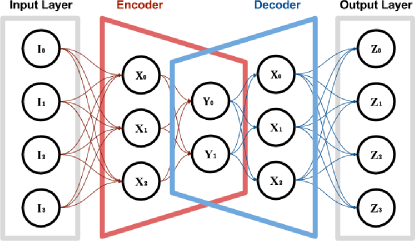
Figure 1: A schematic representation of an autoencoder (image was taken from Ref. AutoEncoderImage ).

An autoencoder consists of two segments of neural network. The first segment is called the encoder, which leads to a bottleneck with the number of nodes being less then the input. The second segment is a decoder which takes the output from the encoder bottleneck and tries to reconstruct the original input at the final output. In the simplest case, both encoder and decoder are fully connected (dense) neural networks, but can also be constructed by convolution layers. In this study we consider both fully connected and convolution autoencoders 726791 ; Masci2011StackedCA , note that the size of the bottleneck is an important characteristic of the autoencoder.

A schematic diagram representing a dense autoencoder is shown in Figure 1, it consists of multiple layers of fully connected neural networks with the output of one layer serving as input to the next layer:

$$O_{i}^{L}\ =\ \sigma\left(\sum_{j}W_{ij}^{L}I_{j}^{L}+B_{i}^{L}\right)\;,$$ (12)

where, $O_{i}^{L}$ and $I_{j}^{L}$ are the output and input vectors respectively, $W_{ij}^{L}$ is the weight matrix, and $B_{i}^{L}$ is the bias vector for the neural network layer $L$. Note that, for internal layers $I_{j}^{L}$ is the output from the previous layer, or $I_{j}^{L}=O_{j}^{L-1}$. Finally, $\sigma$ is the activation function. We use ReLU RIS_0 as the activation functions for all the intermediate layers and SoftMax for the final layer defined as

$$\text{ReLU}\left(x_{i}\right)\ =\ \begin{cases}0&\mbox{if}\quad x_{i}<0\\ x_{i}&\mbox{otherwise}\end{cases}\;,\qquad\text{and}\qquad\text{SoftMax}\left(x_{i}\right)\ =\ \frac{e^{x_{i}}}{\sum_{j=1}^{N}e^{x_{j}}}\;.$$ (13)

Further note that the weight matrix $W_{ij}^{L}$ is of dimension $M^{L}\times N^{L}$, where $M^{L}$ is the dimension of the output vector $O_{i}^{L}$ and $N^{L}$ is the dimension of the input vector $I_{j}^{L}$. For an example, in the first layer, $N^{1}={N_{H}}^{2}$. Given a network with $K$ layers, we additionally impose $M^{K}=N^{1}$, which ensures that the final output vector has the same dimensionality as the input and hence can be readily compared. Also, since we use SoftMax for the final layer, we ensure that the final output (namely, $O_{i}^{K}$), is also a discrete probability distribution function. This allows us to compare the final output to the initial image by a simple $L_{2}$ norm function, which we use as the autoencoder loss function per input vector:

$$\epsilon\ \equiv\ \sqrt{\sum_{i}\left(O_{i}^{K}-I_{i}^{1}\right)^{2}}$$ (14)

Similarly, a convolution autoencoder can be constructed by using convolution (Conv) and convolution transpose (ConvTrans) networks instead of dense networks in the encoder and decoder segments respectively. Numerically, the (discretized from the integral definition) convolution operation takes the form:

$$O_{m,n} = \sum_{i,j}W_{i,j}I_{\left(m+i\right),\left(n+j\right)}$$

where, the limits of the sum are determined based on the input and output dimensionality. Here, the indices of the weight matrix can also take negative values. Max pooling layers (MaxPool) are used to down-sample the image further in between the convolution layers, max pooling layer basically returns the maximum among all the input pixels. Convolution transpose layers do the reverse of convolution layers in the sense that intensity of a single input pixel is added to all the output pixels.

We describe the details of the actual architecture of the convolutional autoencoders later in Appendix D. Even though we focus on the simplest form of autoencoders, there have also been various improvements to the autoencoder brought in by variational decoding 2013arXiv1312.6114K or adversarial training 2017arXiv170104722M . For further information see references and articles cited in Refs. 726791 ; Masci2011StackedCA ; 2011arXiv1106.1925P ; Monk:2018zsb ; Farina:2018fyg ; Heimel:2018mkt ; 2013arXiv1312.6114K .

2.3 Summary of the whole algorithm

Before concluding this section, we summarize the full algorithm in brief:

• Start with jets clustered using any of the standard IR-safe jet algorithms. We represent the jet momentum by $P_{J}^{\mu}$ and its constituent momenta by $p_{i}^{\mu}$ (see Eq. (1)).

• Rescale $p_{i}^{\mu}$ (and as a result $P_{J}^{\mu}$) such that the the new jet momentum $P_{J}^{\prime\mu}$ is characterized by a given mass $m_{0}$. We also denote the rescaled component momenta by $p_{i}^{\prime\mu}$ (see Eq. (2)).

• Lorentz boost either parallel or anti-parallel to the jet momenta as prescribed in Eq. (3) such that the energy of the jet in the new frame is given as a predetermined $E_{0}$. The boost factor required is given in Eq. (6). We denote the jet momentum and the constituent momenta in the new frame by $\mathbf{P}_{J}^{\mu}$ and $\mathbf{p}_{i}^{\mu}$ respectively.

• Find the optimal set of basis vectors $\left\{\hat{e}_{1},\hat{e}_{2},\hat{e}_{3}\right\}$ as described in Eqs. (7 - 9). The vectors $\hat{e}_{2}$ and $\hat{e}_{3}$ span the plane transverse to the jet axis, which is given by $\hat{e}_{1}$.

• Use the constituent momenta $\mathbf{p}_{i}^{\mu}$, and the basis vectors $\hat{e}_{2}$ and $\hat{e}_{3}$, to construct the final jet image (or rather a 2D histogram) of a given size $N_{H}\times N_{H}$ by using Eq. (10).

• For the convolution autoencoder use the image (a 2D histogram) as input. On the other hand, for the dense autoencoder flatten the image to make a one dimensional array and use it as the input.

3 Results

Before proceeding, note that our tasks are divided into two main categories:

1. The main task is to show that our procedure is robust. The robustness feature reflects the fact that the autoencoder loss function as defined in Eq. (14) does not vary as jets from different $\rho$ bins are used to train the autoencoder.

2. Also we benchmark the performance of our method as an anomaly finder. We carry this out in two parts:

   1. In the first part, we treat top-jets and $W$-jets as anomalies. This also allows us to compare the performance of our method with tools based on physics information, as well as with previous proposals.

   2. In the second part, we benchmark the performance of our method after introducing a NP particle decaying to di-$W$-jets giving rise to jets consisting of decay products of two $W$-bosons.

In the rest of this section we begin with the simulation details in Subsec. 3.1, while results for task 1 and task 2 are presented in Subsec. 3.2 and Subsec. 3.3 respectively.

3.1 Simulation Details

In this study we generate all events using PYTHIA8-8.2.26 Sjostrand:2006za ; Sjostrand:2014zea and use Delphes-3.4.1 deFavereau:2013fsa to simulate detector environment. We compare results before and after adding various levels of complexity, such as turning on multi parton interaction (MPI) or detector effects.

We begin by clustering final state detectable particles from the output of PYTHIA8 into jets Anti-$k_{t}$ Cacciari:2008gp of $R=1.0$ using fastjet-3 Cacciari2012 . We only consider the hardest jet from an event in the central region $\left|{\eta}\right|<2.0$. On the other hand, we use eflow elements such as tracks, neutrals and photons from the output of Delphes to find jets, when we simulate detector effects.

The jet mass and transverse momentum we have considered in our study vary over a wide range as discussed later. Using these jets as input, jet images are formed using the method detailed in Subsec. 2.1 with the parameters $m_{0}=1/2$ GeV, $E_{0}=1$ GeV and $N_{H}=40$. The full structure of the network can be read from the source code linked at the end of the document.

• Arch-1: This is a large, dense autoencoder. Basically the input consists of a $40\times 40$ pixel flattened image, each layer decreases both the row and column by 7 until the narrowest bottleneck of $5\times 5$ is reached. The network expands in the same way again by 7 for both column and row, each layer has the ReLU activation, only the final layer has a softmax activation. We try to give a short hand notation for the structure of our network in Figure 2. Most of the results in this article are presented for this architecture of autoencoder.

• Arch-2: This is a shallow dense autoencoder, again the number of inputs is $40\times 40$ pixel flattened image. The structure is shown in Figure 3, as before, SoftMax activation is used in the final layer and ReLU activation is used for every other layer. We have mainly used this architecture of autoencoder to benchmark and verify that the results we observe are also reproducible using a much simpler autoencoder.

• Arch-3: This is a deep convolution autoencoder, the input image shape is $\left(1,40,40\right)$. Its architecture is described in Appendix.C. We mainly use this architecture of autoencoder to benchmark the robustness of our method and find that, even though it performs slightly worse than the above two architectures, it is also more robust than both of them.

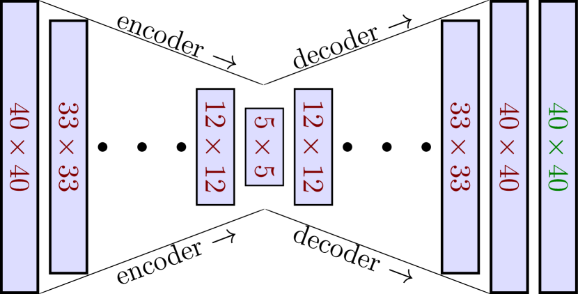
Figure 2: A schematic of the autoencoder structure used in our work (Arch-1). Layers with text in red have ReLU activation while the last layer with text in green has SoftMax activation (see Eq. (13)).

Figure 3: A schematic of the autoencoder structure used in our work (Arch-2). Layers with text in red have ReLU activation while the last layer with text in green has SoftMax activation (see Eq. (13)).

Note that the jet image used as input to the autoencoder is normalized to 1 and each bin (pixel) is non-negative, i.e., it represents a discrete PDF. These properties might be lost when the image is propagated through the neural network. The softmax activation is used in the last layer to restore the normalization of energy clusters and also to make them non-negative. This forces the network to learn the main features of the image instead of just reproducing the magnitude and improves the overall training speed.

We arrive at these structures by checking through a few configurations mainly determined by the size of the bottleneck and settled on these architectures, as increasing it further did not yield any significant improvement on reconstruction (loss function) of QCD in the first few training epochs. Also, for training this network, we use the Adam DBLP:journals/corr/KingmaB14 gradient descent with a batch size of around 100 to 200 and learning rate (step size of the gradient descent) of around 0.001 to 0.0001.

We have written and trained the network using the gluon API of Apache MXNet 2015arXiv151201274C in python. This was chosen over TensorFlow DBLP:journals/corr/AbadiABBCCCDDDG16 because of superior training performance on the CPU and easier imperative API, although we verified that the results are similar between this and TensorFlow using both the TFLearn DBLP:journals/corr/Tang16d andx Keras wrapper API.

3.2 Robustness

The main goal of this section (as stated before) is to establish that the autoencoder loss function obtained using our method is rather insensitive to the jet masses of the control sample. We demonstrate this is by training the autoencoder network on QCD-jets from a particular region of the phase space and by testing the trained network on QCD-jets from a different region of the phase space, we divide our result into three parts:

1. We train the autoencoder network on QCD-jets with $800~{}\text{GeV}<{p_{T}}_{J}<900~{}\text{GeV}$ produced at $\sqrt{s}=13~{}\text{TeV}$ collision energy (with no cuts on the jet mass). The data is then divided into bins depending on jet masses. The loss function (from the autoencoder trained in the previous step) is evaluated on events from each bin and compared with each other as well as with the distribution of the whole sample (Subsec. 3.2.1).

2. We use QCD-jets produced at $\sqrt{s}=100~{}\text{TeV}$ with ${p_{T}}_{J}>10~{}\text{TeV}$, and then divide the full sample into bins depending on jet masses. We train an autoencoder network using QCD-jets from one of these mass bins and test with the others (Subsec. 3.2.2).

3. As extreme comparions, we train on jets from $\sqrt{s}=13~{}\text{TeV}$ collider, and test on data from $\sqrt{s}=100~{}\text{TeV}$ collider, and vice versa. The results from this study is shown in Appendix A.

3.2.1 Robustness at $\sqrt{s}=13$ TeV

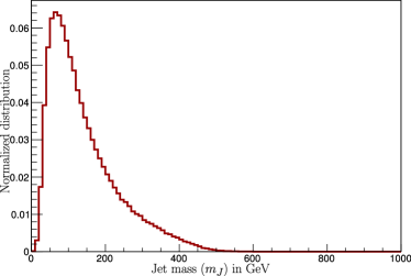
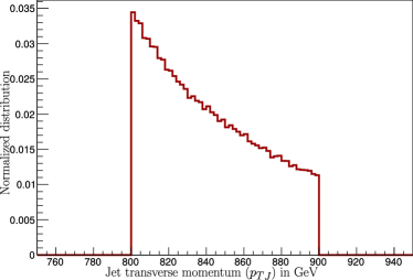
Figure 4: The mass (left) and transverse momentum (right) distribution of jets we use for our study.

In this part, we study QCD-jets at $\sqrt{s}=13$ TeV. To be particular, we consider QCD di-jet events and study the jet hardest in $p_{T}$ from each event. We begin by studying jets with $800~{}\text{GeV}<{p_{T}}_{J}<900~{}\text{GeV}$ generated without MPI. The jet mass and transverse momentum distribution of the sample is shown in Figure 4. The transverse momentum distribution is, as expected, lying in the window of 800 GeV to 900 GeV due to the imposed phase space cuts and the jet mass gives the expected falling distribution.

The jet images (as explained in Subsec. 2.1.3) are basically a map from a set of two dimensional integers (representing the pixels or the bins $\left(I,J\right)$) to the set of real numbers between 0 and 1 (representing the intensities, $F_{IJ}$) given by Eq. (10).

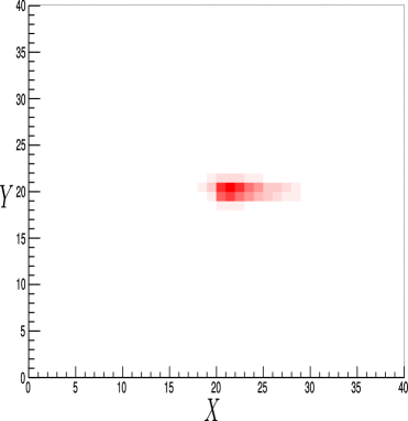
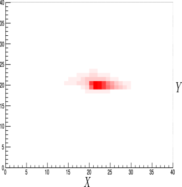
Figure 5: The image of a QCD-jet (averaged over $\approx 500000$ jets) obtained after our pre-processing method without(left) and with(right) detector effects (using Delphes). The image is a 3D plot with the color density (the $z$ axis) representing intensity. To be specific, the axis represent: $\left(x,y,z\right)\rightarrow\left(I,J,\langle F_{IJ}\rangle\right)$, the axis labels follow the convention in Eq. (10).

In Figure 5, we present the averaged (over $500000$ jets) jet image of QCD-jets using our method. The color intensity of a bin (pixel) with coordinate $\left(I,J\right)$, represents the average $\langle F_{IJ}\rangle$ (the intensity of each pixel or bin is averaged across many jets). The averaging procedure captures the broad features of the event type while smoothing over sharp fluctuations from individual events.

The image faithfully reproduces the simple dipole emission structure of QCD-jets, where the hardest emission from the parton initiating the jet decides the major (elongated) axis of the jet (which is brought along the $x$ axis of the image Figure 5 due to the Gram-Schmidt procedure in Eq. (8)) while most subsequent emissions tend to lie along this axis (owing to the color connected Gallicchio:2010sw structure of QCD interactions). We also observe that the main impact of detector simulation seems to smear the energy distribution of the jet constituents.

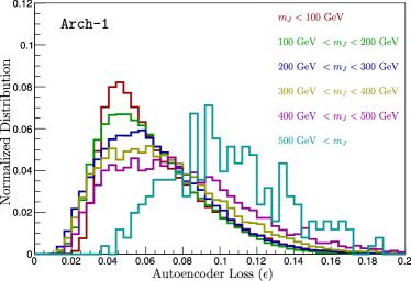
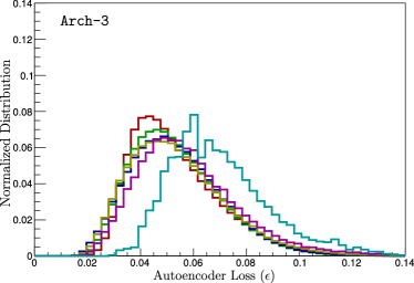
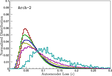
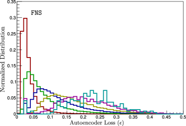
Figure 6: The effect of mass cuts on the autoencoder response (for QCD-jets) using our method for Arch-1 (top-left), Arch-2 (bottom-left), Arch-3 (top-right) and using the dense autoencoder from Ref. Farina:2018fyg (lower-right).

At this point, we train the autoencoder network on the full set of jets without any cut on the jet mass and then test the variation of the autoencoder loss function on various mass bins. We present the result of these studies in Figure 6, where we plot the autoencoder loss functions for all the three architectures as jets are analyzed using various mass bins. We compare these with responses of dense autoencoder from Ref. Farina:2018fyg to calculate loss function (bottom-right plot of Figure 6). Clearly, our method yields better robustness. The change in the peak position of the autoencoder loss distribution for different jet masses using our method (for Arch-1) is within $10\%-15\%$. On the other hand, when we use the method from Ref. Farina:2018fyg , the peak position shifts by factors of $4$ to $5$. Similar trends are also seen in the widths of the distribution which hardly changes for different mass bins when using our method while changing significantly (by several factors) for the method proposed in Ref. Farina:2018fyg . Although, we have compared only the dense autoencoder from Ref. Farina:2018fyg here, the robustness of convolution autoencoders are found to be only slightly better (order $30\%$ for $m_{J}>300$ GeV) Farina:2018fyg . However, as one can see from the lower-right plot of Figure 6, 20% to 30% improvement is not sufficient. Our simple method is significantly more robust.

A comparison of the three architectures used in this work is warranted. The convolutional autoencoder gives significantly more robust performance than any of the other autoencoders using dense networks. As noted before, this observation was also mentioned in Ref. Farina:2018fyg . Note also that the shallower dense network employed in Arch-2 yields substantially more robust features than that of Ref. Farina:2018fyg , even though it is worse than the deeper dense network in Arch-1.

This de-correlation of loss and jet mass is an extremely interesting phenomenon and deserves more attention. This feature can also be demonstrated in the distributions of jet masses where jets are binned in loss $\epsilon$. In Figure 7, we show these jet mass distributions in bins of $\epsilon$. To be specific, we follow the procedure as outlined in Heimel:2018mkt and choose a cut on $\epsilon$ dynamically such that only a given fraction (say, $\mathcal{F}$) of QCD-jets pass this cut. The jet mass distribution for these passed jets are then plotted, The procedure is repeated for different values of $\mathcal{F}$. We show the results of these studies in Figure 7, where jet mass distributions remain robust for all the three architectures. Only for $\mathcal{F}<0.05$ we start seeing deviations and the three architectures show slightly different results. Not surprisingly, the convolutional autoencoder (Arch-3) produces the best result in that even for $\mathcal{F}<0.05$ the jet mass distributions are virtually identical. The $\mathcal{F}<0.05$ plot of deeper dense network in Arch-1 shows some variation from other $\mathcal{F}$ plots, and the difference is more enhanced for the shallower dense network in Arch-2.

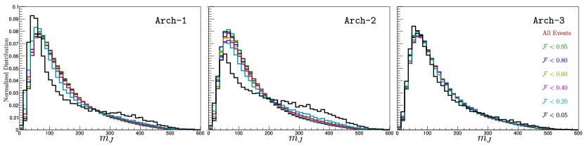
Figure 7: The distribution of jet mass in bins of autoencoder loss.

It is tempting to compare the robustness presented in Ref. Heimel:2018mkt , where the authors use additional adversarial training to decorrelate QCD-jets from jet masses. Our method, relying largely on physics driven preprocessing gives as robust a performance as the proposal in Ref. Heimel:2018mkt . We perform additional checks to pin down the exact reason behind the observed de-correlation effect between the autoencoder loss and the jet mass. In order to quantify it, we use the usual linear correlation coefficient. Given two variables $A$ and $B$, the linear correlation coefficient, denoted by $\rho(A,B)$, is defined by the following equation

$$\rho\left(A,B\right) \equiv \frac{\left\langle AB\right\rangle-\left\langle A\right\rangle\left\langle B\right\rangle}{\sqrt{\left\langle A^{2}\right\rangle-\left\langle A\right\rangle^{2}}\sqrt{\left\langle B^{2}\right\rangle-\left\langle B\right\rangle^{2}}}$$ (15)

where $E(A)$, $E(B)$, and $E(AB)$ represents the expectation values of the variables $A$, $B$, and $AB$ respectively. In order to demonstrate how the loss becomes de-correlated as we perform various stages during preprocessing of jets, we calculate $\rho(\epsilon,m_{J})$ in four different studies:

1. Preprocessing without Lorentz boost + a fully connected network Arch-1 for the autoencoder.

2. Preprocessing without using Gram-Schmidt axis + a fully connected network Arch-1 for the autoencoder. Note that, unfortunately, due to the (arbitrary) rescaling and boosting steps, it no longer makes sense to use the usual $\eta$ and $\phi$ coordinates. Gram-Schmidt remains the only sensible way to pick the basis in the transverse plane (to the jet axis). Here we attempt to estimate the effect of using Gram-Schmidt by using an arbitrary basis vectors instead of the hardest constituent (or subjet) vectors.

3. Full preprocessing + a fully connected network Arch-1 for the autoencoder.

4. Full preprocessing + a convolutional autoencoder Arch-3 for the autoencoder.

CASE	Correlation between $\epsilon$ and $m_{J}$
1: No Lorentz Boost + Arch-1	75
2: Random Gram-Schmidt Axis + Arch-1	32
3: Full pre-processing + Arch-1	7
4: Full pre-processing + Arch-3	2

Table 1: The linear correlation coefficients $\rho(\epsilon,m_{J})$ (in $\%$) for the four cases mentioned in the text: preprocessing without Lorentz boost + Arch-1 (first from left), preprocessing without using Gram-Schmidt axis + Arch-1 (second), full preprocessing + Arch-1 (third), and finally, full preprocessing + Arch-3 (fourth).

The results are shown In Table 1. It is clear that the largest impact of de-correlation comes from performing the Lorentz boost during preprocessing. Using Arch-1 for the autoencoder, one improves $\rho(\epsilon,m_{J})$ from $75\%$ to $7\%$ if the Lorentz boost step is performed (compare the first and third rows in Table 1). The effect of using Gram-Schmidt axes is rather mild. Using arbitrary axes, instead of Gram-Schmidt axes, deteriorates $\rho(\epsilon,m_{J})$ from $7\%$ to $32\%$ (compare the third and second rows in Table 1). Finally, as seen in previous figures, we see modest improvement as we change from Arch-1 to Arch-3 -- a gain in $\rho(\epsilon,m_{J})$ from $7\%$ to $2\%$ is seen when we compare the last two rows in Table 1. For the full 2-dimensional distribution of autoencoder loss $\epsilon$ as a function of jet mass $m_{J}$ observed in these studies, see Appendix B.

Note that throughout Subsec. 3.2.1 we have shown results after dividing the testing sample in bins of jet masses, whereas the training sample had no such binning. In other words, the training dataset, in principle, contain information of jets of all masses. A rather more stringent test is to train using jets from a particular bin of jet masses, and test with jets from different bins. Operationally, it is more convenient to use jets produced at much higher center of mass energy collisions since, as shown in Figure 4, the sample we work with (at $\sqrt{s}=13$ TeV) is characterized by a rather shallow range in jet masses. We, therefore, leave this study for the next section where jets are produced at $\sqrt{s}=100$ TeV collisions.

3.2.2 Robustness at $\sqrt{s}=100$ TeV

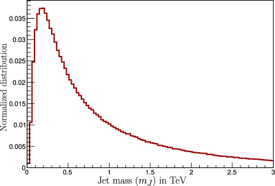
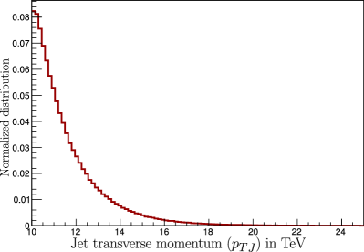
Figure 8: The mass (left) and transverse momentum (right) distribution of jets we have used for our study at $\sqrt{s}=100$ TeV.

In this subsection we study the robustness with QCD-jets of high transverse momentum and jet mass. For this purpose, we consider jets with ${p_{T}}_{J}>10~{}\text{TeV}$ from QCD-dijet events at a $\sqrt{s}=100~{}\text{TeV}$ collider, generated without MPI. For these event we do not simulate any detector effects. The $m_{J}$ and ${p_{T}}_{J}$ distributions of these jets are presented in Figure 8. Note the broad range of jet mass distribution of the dataset. It allows us to divide the training sample into a large number of bins of different jet masses while still keeping statistics under control.

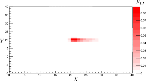
Figure 9: The image of QCD-jets at $\sqrt{s}=100~{}\text{TeV}$ obtained using our method without MPI or detector effects (the axis labels follow the convention in Eq. (10)).

Before beginning, we show the average image of these jets obtained after our preprocessing steps in Figure 9. Clearly, the image is almost identical to the image in Figure 5 obtained for QCD-jets from $\sqrt{s}=13~{}\text{TeV}$ collisions further fortifying our claims. Note that the most energetic part of the image (as measured using the scales on the $x$ and $y$ axis) is identical between Figure 5 and Figure 9. This demonstrates that our method always resolves the jet at the same length scales irrespective of the jet mass or momentum (boost).

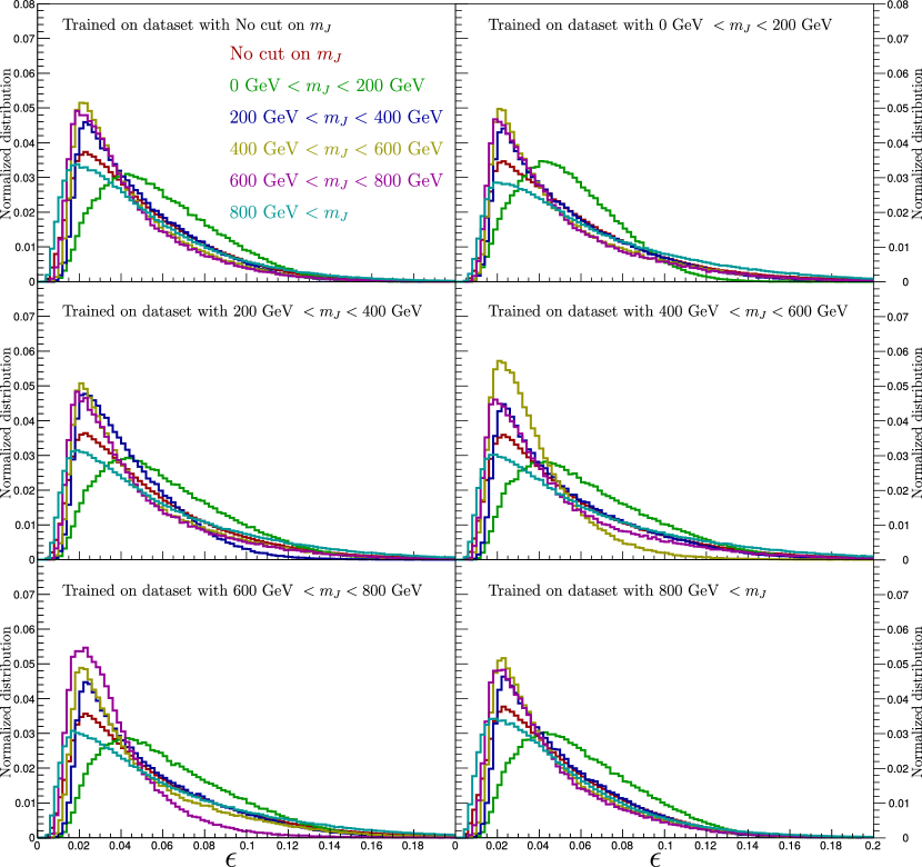
Figure 10: The (normalized) distribution of autoencoder loss function for QCD jets (${p_{T}}_{J}>10~{}\text{TeV}$) in various mass bins, the autoencoder with jets in a particular mass bin (indicated in each of the figures) and tested on all the other mass bins. The colors of the histogram represent the mass bins as labeled.

Note that the purpose of this section is to check the robustness of our methodology, where we train jets from a given bin of jet masses while we test it with jets from different bins. We begin by dividing the full set of jets into subcategories according to:

1. No cut on $m_{J}$ (all jets are considered)

2. $m_{J}<200\text{ GeV}$

3. $200\text{ GeV }<m_{J}<400\text{ GeV}$

4. $400\text{ GeV }<m_{J}<600\text{ GeV}$

5. $600\text{ GeV }<m_{J}<800\text{ GeV}$

6. $800\text{ GeV }<m_{J}$

In all of these cases, we form images using our method and analyze further using the autoencoder in various permutations. In order to check for robustness, we use the following strategy:

1. Train an autoencoder on jets from each of the mass bins mentioned above.

2. Evaluate the performance of these networks on jets from each of the mass bins listed above.

We only use the dense network in Arch-1 for the autoencoder. The comparative studies between different architectures as well as with/without various stages of preprocessing is already presented in Subsec. 3.2.1 and we do not repeat these here. We show the results from this study in Figure 10, where we plot distributions of loss-functions for jets (in various bins of jet masses). All of these figures again strongly support the claim that our method mostly eliminates the dependence of jet mass on the autoencoder loss function. As can be observed from the distributions Figure 10, most of the peak position lie within $\approx 20\%$ of each other and the distributions largely overlap.

At this point, we do not show any more plots (such as distributions of jet masses in bins of loss) to demonstrate the robustness feature in our proposal. As shown in Subsec. 3.2.1, robustness in the distribution of $\epsilon$ for various $m_{J}$ bins immediately implies robustness in the distribution of $m_{J}$ for various $\epsilon$ bins.

The lesson from all these different studies in Subsec. 3.2.1 and Subsec. 3.2.2 is rather straight-forward: our (physics-driven) proposal to preprocess jets before it is subjected to an autoencoder, manages to de-correlate jet masses from jets successfully, yielding a robust methodology that can look for jets with high masses as anomalies while only being trained on jets of low masses.

3.3 Performance

The task in this subsection is to examine and benchmark the performance of our method as an anomaly finder for various types of standard jets. As stated before, the autoencoder loss function can be used as a measure to determine how different a jet ‘‘looks like’’ as compared to the QCD-jets on which the autoencoder was trained on. Apart from considering top-jets and $W$-jets as anomalies, we also examine the performance of our method when these anomalous jets are due to new physics. In particular, we study jets containing decay products of two hadronically decaying $W$-particles (namely, di-$W$ jet). The $p_{T}$ and jet mass distributions of jets in these datasets are shown in Figure 11. As shown in Figure 11, all jets in this discussion are characterized by a $p_{T}$ in the range $800~{}\text{GeV}\leq p_{T}\leq 900~{}\text{GeV}$. The jet mass distributions for top jets, $W$-jets, and di-$W$-jets are peaked nicely near top-mass, $W$-mass, and the di-$W$ resonance (we take it to be $180~{}\text{GeV}$).

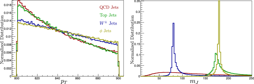
Figure 11: The $p_{T}$ and jet mass distributions for jets in different datasets.

We first train the autoencoder using QCD-jets. Note that once the training on QCD-jets are done, the trained autoencoder acts as a so-called ‘‘black-box" which, given any jet simply associates with it a loss $\epsilon$. The loss function for these three different jet types (we use an autoencoder with the dense network in Arch-1) is presented in Figure 12. We do not use MPI or detector effects in order to produce these plots, the purpose of which are simply to demonstrate that the loss $\epsilon$, by itself, can identify jets of any of these three types as anomalous jets. It is clearly seen that the autoencoder loss increases as more complex structure is added to the jet. QCD-jets (on which the autoencoder was trained on and also have the simplest 1-prong dipole emission substructure) have, on average, the smallest loss function. $W$-jets, on the other hand, have a 2-prong structure which is slightly more ‘‘complex’’ than the 1-prong QCD-jet structure, and therefore have larger loss functions on average. Top jets come next in the hierarchy as they mostly have a 3-prong structure (with an onshell $W$) making it more ‘‘complex’’ than a $W$-jet. Finally, we show jets originating due to boosted $\phi\rightarrow W^{+}W^{-}$. This gives rise to jets with 4-prong structure (containing 2 on-shell $W$ resonances in the same jet). Not surprisingly, we find these jets with the highest loss functions.

Figure 12: The autoencoder loss function ($\epsilon$, Eq. (14)) obtained from the autoencoder using our method of pre-processing for the case with no detector effects or multi parton interaction.

In order to quantify the comparison between the performance of various methods, we compare the receiver operating characteristic (ROC) curves. In our study, these curves are presented with the convention that the $x$ axis represent the signal selection efficiency and the $y$ axis represent the reciprocal of the background fake rate (in log scale). Therefore, the algorithm producing curves closer towards the top right region of the graph would mean a better performing algorithm. It is also possible to compare two algorithms based on the area under the ROC curves of the two algorithms, larger area would generally mean better performance.

Next, we examine each of the cases in greater detail, benchmarking our method against some standard techniques which are well established and also against some recent techniques found in literature.

3.3.1 Benchmark with top jets

The problem of discriminating jets originating from boosted tops against jets from QCD is extremely well studied theoretically Dasgupta:2018emf ; Dasgupta:2013ihk ; Dasgupta:2013via ; Marzani:2019hun , numerically Plehn:2011tg ; Kasieczka:2015jma ; Plehn:2010st ; Kaplan:2008ie ; Plehn:2009rk ; Thaler:2011gf and experimentally CMS:2014fya ; Aaboud:2018psm . Let us reiterate that the purpose of the subsection is not to promote the loss of an autoencoder, which is trained entirely on QCD jets, to be an efficient top-tagger. Since the autoencoder loss has no information about top jets, it is expected to under perform when compared to any decent top-tagger, which uses information specific to top decays. By treating top-jets as anomalies in this exercise, we rather hope to measure qualitatively the efficiency of this proposal if indeed we encounter anomalous jets (for an example, a jet consisting of decay products of a new beyond the standard model particle). Indeed, earlier work on anomaly detection Farina:2018fyg ; Heimel:2018mkt also used top jets as anomalies in order to benchmark. In this subsection we take an identical approach to establish the performance of the dense and convolution autoencoder loss functions and compare it with the one in Ref. Farina:2018fyg , while also showing the performance of HEPTopTagger2 Plehn:2011tg ; Kasieczka:2015jma ; Plehn:2010st ; Plehn:2009rk in parallel as it is a well understood technique.

Top jets are obtained from $t\bar{t}$ events as detailed in Subsec. 3.1. We present the results for three main cases:

1. Top jets with $800~{}\text{GeV}<{p_{T}}_{J}<900~{}\text{GeV}$ simulated without MPI or detector effects.

2. Top jets with $800~{}\text{GeV}<{p_{T}}_{J}<900~{}\text{GeV}$ simulated without MPI but with detector effects.

3. Top jets with ${p_{T}}_{J}>400~{}\text{GeV}$ simulated with MPI and detector effects.

While generating these events in cases. (A) and (B), we impose an additional merge requirement between the jet and the partonic top along with its decay products $\left({b,q,{\bar{q}}^{\prime}}\right)$ by demanding that they lie within the jet at PYTHIA8 level.

$$\begin{split}{\Delta}R{\left({p_{J}^{\mu},p_{\text{top}}^{\mu}}\right)}\ <\ 0.6&\qquad\qquad{\Delta}R{\left({p_{J}^{\mu},p_{q}^{\mu}}\right)}\ <\ 0.6\\ {\Delta}R{\left({p_{J}^{\mu},p_{b}^{\mu}}\right)}\ <\ 0.6&\qquad\qquad{\Delta}R{\left({p_{J}^{\mu},p_{\bar{q}^{\prime}}^{\mu}}\right)}\ <\ 0.6\;,\end{split}$$ (16)

Which ensures a consistent comparison with Ref. Farina:2018fyg . The merge requirement is not imposed for case. (C).

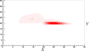
Figure 13: The images of top-jets (averaged over $\approx 500000$ events) obtained after our preprocessing method without (left) and with (right) detector effects (using Delphes), the axis labels follow the convention in Eq. (10).

The jet images obtained using our method with and without detector effects are shown in Figure 13, clearly the structure is much more ‘‘complex’’ than the case of QCD jets. Even though the three prong structure is not pronounced (due to the three body decay) in the image, it is still visible in a subtle way. The extended horizontal lump and lobe approximately constitute two prongs while the third is from the vertical extension of the lobe towards the left. Again, the effect of detector simulations seem just to smear the momentum distribution of the jet constituents.

Note that the difference in distributions of top jets and QCD-jets suggest that simple cuts on the loss $\epsilon$, can be helpful in order to find top jets as anomalies. For example, if we consider jets with $\epsilon>\epsilon_{\text{cut}}$, where $\epsilon_{\text{cut}}=0.15$, to be signals (i.e., outliers as far as QCD-jets are concerned) we find that a negligible fraction of QCD-jets (namely $\epsilon_{\text{QCD}}$) and a rather large fraction of top-jets (namely $\epsilon_{t}$) pass the cut. Varying $\epsilon_{\text{cut}}$, one obtains $\epsilon_{t}$ as a function of $\epsilon_{\text{QCD}}$ (the ROC for top jets).

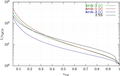
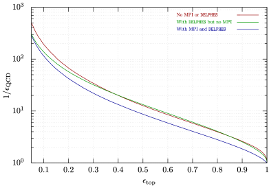
Figure 14: ROC Comparing the three architectures of the autoencoder along with the method from Farina:2018fyg for QCD vs top jet discrimination using only autoencoder loss (left) and ROC comparing the effects of MPI and detector effects on Arch-1 of the autoencoder (right).

In the left plot Figure 14, we compare the ROCs produced by autoencoders using network architectures in Arch-1, Arch-2 and Arch-3. Clearly, the dense network in Arch-1 offers the best performance but is closely followed by much shallower Arch-2. Even though the convolutional autoencoder in Arch-3 is the most robust anomaly finder (as seen in Figure 6, Figure 7, and Table. 1), it does not offer as good a performance to identify top-jets as anomalies.

A potentially interesting example is to use the loss function $\epsilon$ in a supervised manner. As mentioned before, after training on QCD-jets, the trained autoencoder can be taken to be a ‘‘black-box" where for any input jet the black-box gives an output loss $\epsilon$. One can use this $\epsilon$ as a jet-shape like any other physics based ones (such as mass or $N$-subjettiness), even though it is hard to interpret. In the problem of finding top jets, therefore, we can combine $\epsilon$ and $m_{J}$ in the sense that we can introduce rectangular cuts on the $\epsilon$--$m_{J}$ plane to calculate $\epsilon_{t}$ and $\epsilon_{\text{QCD}}$. In order to perform this study on the $\epsilon$--$m_{J}$ plane in a systematic manner and produce ROCs we use a Boosted Decision Tree (BDT) based multivariate analysis as implemented in Root BRUN199781 , which simply finds signal rich hypercubes (here rich in top-jets) in multi-dimensional spaces of observables (here the $\epsilon$--$m_{J}$ plane), which are rich in signal (here top jets). The results of these studies are presented in Figure 15.

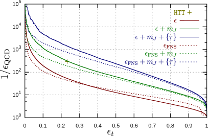
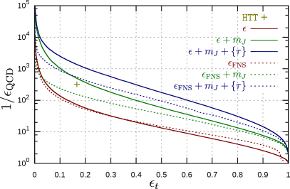
Figure 15: ROC for discriminating QCD vs.top using our auto encoder loss function $\epsilon$, as well as combining $\epsilon$ with jet mass and N-subjettiness variables $\{\tau_{1},\dots,\tau_{5}\}$. For comparison, we also produce the same but using $\epsilon_{\text{FNS}}$, loss functions trained using Ref. Farina:2018fyg . These results are presented without (left) and with (right) detector effects.

In order to demonstrate that our pre-processing step does not degrade the performance, we compare ROCs with and without pre-processing. To be specific, we compare the ROC produced using cuts on $\epsilon$, where we use the pre-processing stage and employ the architecture in Arch-1, with that of the dense network of Ref. Farina:2018fyg without preprocessing (we refer to it as $\epsilon_{\text{FNS}}$). As shown in Figure 15, both these ROCs are comparable. In the same figure, we also show the discriminating power of the well-studied, well-understood HEPTopTagger2 Plehn:2011tg ; Kasieczka:2015jma ; Plehn:2010st ; Plehn:2009rk by the point marked ‘‘$+$’’ in the plot. Note that the default version functions without Qjets Ellis:2014eya ; Ellis:2012sn or any other variables (like N-subjettiness Thaler:2011gf or Energy Correlation Larkoski:2013eya ), but uses the jet mass information in the mass drop step and also many other features from the physics of top quark decay kinetics. Clearly, HEPTopTagger2 Plehn:2011tg ; Kasieczka:2015jma ; Plehn:2010st ; Plehn:2009rk outperforms the autoencoder when we only use cuts on $\epsilon$. This is completely understandable since the autoencoder uses no physics information associated with top decays. The fact that one still achieves the impressive performance to find top jets as anomalies is impressive. As a further demonstration we additionally show ROCs where we combine $\epsilon$ with $m_{J}$ and $N$-subjettiness $\{\tau_{1},\dots,\tau_{5}\}$, by using BDTs. Not surprisingly, we find significantly better performance. It shows that our technique is extremely general and its performance can be competitive with specialized taggers designed for each event topology.

At this point, we also wish to note another important feature in the graph. When just the autoencoder loss is used, $\epsilon_{\text{FNS}}$ does outperform our method in a large portion. But it is worth pointing out that $\epsilon_{\text{FNS}}$ uses a large amount of information from the jet mass as seen from Figure 6 and it is not possible to factor out this effect of jet mass from this method easily. So instead of trying to factor out the effect of jet mass from $\epsilon_{\text{FNS}}$, we instead choose another way to make this comparison fair. This is by incorporating the jet mass as an input observable for both the methods while making the comparison. These arguments could be generalized to include other jet observables in addition to the autoencoder loss so that the fraction of information overlapping between these observables and the autoencoder loss can be gauged.

The detector simulation seems to affect the performance of all three methods by $10\%-20\%$. Using our method, for a signal selection efficiency of $\approx 80\%$, background fake rates as low as $5\%$ to $10\%$ can be achieved. The significant enhancement in the performance of the autoencoder loss when it is combined with $m_{J}$ and $N$-subjettiness, suggests that $\epsilon$ is largely uncorrelated with $m_{J}$ and $N$-subjettiness as well. We already have shown how the preprocessing stage de-correlates the loss from $m_{J}$. Since the $N$-subjettiness variables are usually strongly correlated with $m_{J}$, de-correlating mass should also result in de-correlating $N$-subjettiness.

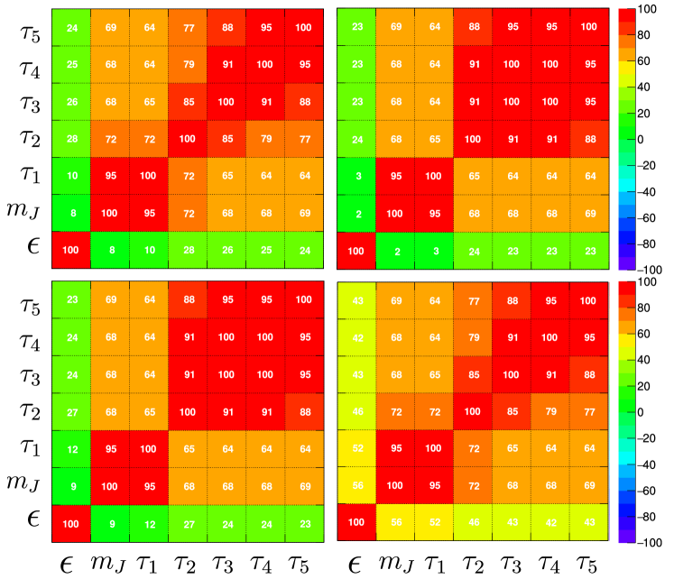
Figure 16: Linear correlation coefficients (in %) among $\epsilon$, $m_{J}$ and $\left\{\tau_{1},\dots,\tau_{5}\right\}$ for QCD-jets using Arch-1 (top-left), Arch-2 (bottom-left), Arch-3 (top-right), and $\epsilon_{\text{FNS}}$ (bottom-right).

In Figure 16 we plot the linear correlation coefficients (in %) among $\epsilon$, $m_{J}$ and $\left\{\tau_{1},\dots,\tau_{5}\right\}$ for QCD-jets using all the three networks discussed in this paper. We see what we expect -- correlation coefficients never reach even $30\%$. In the same figure we also show the same correlation matrix where we combine $\epsilon_{\text{FNS}}$ with $m_{J}$ and $N$-subjettiness variables. As shown in the bottom-right plot, the correlation coefficients for $\epsilon_{\text{FNS}}$ remains in the range $\sim 45\%$ to $65\%$ for all these variables.

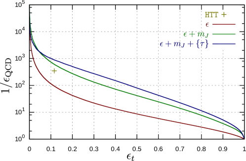
Figure 17: ROC for QCD vs top discrimination using our method with MPI and detector effects.

Finally, in order to demonstrate the fact that our method preserves its performance in a more realistic situation, we benchmark its performance of QCD-jets vs top-jet discrimination on events simulated with MPI and detector effects. We also discard all parton level merge requirements, imposed earlier, as explained in case. (C). Additionally, we use a much larger phase space region with ${p_{T}}_{J}>400~{}\text{GeV}$. We show the results from this study in Figure 17. In the same plot we also show the performance of HEPTopTagger2 for comparison. We see that much of the performance seen in the previous case is still retained even after MPI and detector effects are turned on (see, Figure 15 for comparison).

3.3.2 Benchmark with $W$-jets

In this section, we consider the problem of discriminating $W$ jets against QCD-jets. This is again a well studied problem and variables like $N$-subjettiness Stewart:2010tn ; Thaler:2010tr have been observed to work reasonably well. The CMS collaboration for LHC, for example, used $\tau_{2}/\tau_{1}$ for $W$-tagging Khachatryan:2014vla . We use $W$-jets as anomalies and compare the performance of our methods with that of $\tau_{2}/\tau_{1}$.

In this work we consider a sample of boosted $W$ jets with $800~{}\text{GeV}<{p_{T}}_{J}<900~{}\text{GeV}$, generated without MPI or detector effects. We also impose a merge requirement (as was the case for top) that the parent $W$ and its decay products lie within the jet $\left[\Delta R\left(p_{J}^{\mu},p_{a}^{\mu}\right)<0.6\right]$, where $a$ stands for decaying $W$, as well as quarks from the decay.

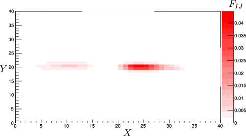
Figure 18: The average jet image of $W$-jet obtained after our pre-processing method (the axis labels follow the convention in Eq. (10)).

Figure 19: ROCs for discriminating QCD-jets vs $W$-jets using our anomaly finder and a standard $N$-subjettiness variable.

The jet images obtained using our method is presented in Figure 18. Notice that the two prong structure of the jet is clearly visible. The asymmetry in the intensities of the two prongs is due to the Gram-Schmidt procedure Eq. (8), which always brings the harder prong along the right side of the horizontal axis by construction.

As before, we use an ROCs to quantify the performance of our method and compare it against an existing standard. The ROC in Figure 19 shows the achievable background rejection efficiency as a function of signal efficiency, when we use autoencoder loss function alone as well as when we combine it with $m_{J}$ and N-Subjettiness variables. We find that our method performs reasonably well as an anomaly finder only when it is combined with the other variables. At the level of $1\%$ QCD-jet reduction it manages to yield a signal selection efficiency of $\sim 20\%$. On the other hand, using $\epsilon$ along with $m_{J}$ and N-Subjettiness as well, yields signal selection efficiency as high as $\approx 60\%$ for the same QCD-jet rejection.

3.3.3 Benchmark with di-$W$ jets from new physics

In this section, we study the efficiency of finding jets consisting of decay products a NP particle (namely $\phi$, a di-$W$ resonance) as anomalies. To be specific, we use a scalar with mass $180~{}\text{GeV}$. We use the effective two Higgs doublet model, where $\phi$ is the heavy scalar Higgs, for generating events. The actual process we consider is given below

$$p\ +\ p\ \rightarrow\ Z\left(\nu_{e}\bar{\nu}_{e}\right)\ +\ \phi\left(W^{+}W^{-}\right)\;.$$ (17)

The events are generated at $\sqrt{s}=13$ TeV without MPI or detector effects. We consider jets with $800~{}\text{GeV}<{p_{T}}_{J}<900~{}\text{GeV}$ that satisfy the usual merge requirement that the heavy parent $\phi$, $W^{+}$, $W^{-}$ and the four final partons lie inside the jet, namely $\left[\Delta R\left(p_{J}^{\mu},p_{a}^{\mu}\right)<0.6\right]$, where $a$ stands for decaying $\phi$, as well as all the partons from $W$-decays.

Figure 20: The average jet image for a di-$W$ resonance with mass $180~{}\text{GeV}$ after our pre-processing method (the axis labels follow the convention in Eq. (10)).

The jet image formed using our method is presented in Figure 20. Even though the four prong structure is not pronounced, it is still visible in a subtle way. As in the case of Figure 13, the horizontal lump and the extended lobe towards the left constitute two prongs while the third and fourth prongs overlap with the first two leading to the halo around the lump towards the right and a bright spot on the left lobe.

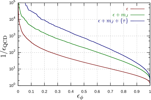
Figure 21: ROC for discriminating QCD vs di-$W$ jets using our anomaly finder.

Finally, we show the ROCs for discriminating these $\phi$-jets as anomalies in Figure 20. The performance of our method is highly promising. Even with just the autoencoder loss, for a signal selection efficiency of $\approx 20\%$, it suffers a fake rate of only $\approx 0.5\%$ due to QCD-jets.

4 Conclusion

In this paper, we propose a new anomaly finder or rather an anti-QCD tagger based on autoencoder. While the proposal uses a version of an autoencoder (without variational or adversarial training), its novelty lies in the preprocessing stage, where we exploit the full Lorentz symmetry apart from symmetries of shift, rotation and rescaling (approximate conformal symmetry of QCD). Our method gives comparable performances to some existing techniques in the literature, while, at the same time, removes the dependence of autoencoder loss function on the jet mass. Consequently, it gives a straight forward way to find pure control samples to train. Our anomaly finder can be trained using jets in low $\rho$ bins, which is rich in QCD-jets, and can be used to analyze jets from high $\rho$ bins to find anomalies (or, signature of NP). The lack of jet mass dependency of the autoencoder loss brings in additional advantages -- it can be readily combined with existing discriminating variables to improve performances of even supervised learning to some effect.

Apart from this robustness feature, we also find that detector effects or multi parton interactions have little effects in the performance of the anomaly finder. We have not explicitly tested our method against pileup in this study. However, we see no reason why this method can not be made pileup robust by simply using the standard pileup mitigation techniques Krohn:2013lba ; Cacciari:2014gra ; Bertolini:2014bba before forming the jet image, or even after the jet image is formed as shown in Ref. Komiske:2017ubm .

We were unable to optimize on the structure of the autoencoder network due to lack of sufficient computational power. However, even with our naive optimization methods, we manage to get remarkable results as compared to existing techniques in literature. Our method provides an extremely simple yet a powerful technique with great potential for generalization as it can be readily incorporated into any existing neural network based algorithms such as image based top tagging Almeida:2015jua ; Macaluso:2018tck ; Kasieczka:2017nvn ; Cogan:2014oua ; Baldi:2016fql ; deOliveira:2015xxd , Lorentz layers Butter:2017cot , or recurrent networks Louppe:2017ipp with minimal effort. Because of its simplicity, the preprocessing stage can even be extended to existing boosted jet substructure classification algorithms that uses only physics information. With more improvements and optimizations, it might even be possible to use the autoencoder loss obtained with our method (combined with the jet mass) as a spectroscopy like observable to find anomalous events.

Source code for most of the content discussed here can be found at: [https://github.com/aravindhv10/CPP_Wrappers/tree/master/AntiQCD4]

Appendix A Cross validation

The purpose of this appendix is to demonstrate that even if the autoencoder is trained using jets in a given $p_{T}$ range, it can still be used to find anomalies in jets with largely different $p_{T}$. To bring home the point we present results from two studies:

1. Train the autoencoder on $\sqrt{s}=13$ TeV QCD-jet data and test it on QCD-jets at $\sqrt{s}=100$ TeV.

2. Train the autoencoder on QCD-jets from $\sqrt{s}=100~{}\text{TeV}$ collisions and test it on the QCD-jets produced at $\sqrt{s}=13$ TeV.

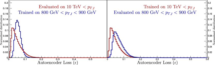
Figure 22: Dependence of autoencoder loss function on jet mass when the network is trained on low energy jets and evaluated on high energy jets (left) and when network is trained on high energy jets and evaluated on low energy jets (right).

Even with these extreme comparisons of jets with drastic differences in kinematics, our method yields largely insensitive results as can be seen in Figure 22. Note that the shift in peak positions in both cases are less than 50% of the width. Most of the actual distributions overlap and, consequently, widths and averages in all cases are within $20\%$ of each other.

Appendix B Autoencoder loss and jet mass

As mentioned in the text, we show the full 2-dimensional distribution of autoencoder loss $\epsilon$ as a function of jet mass $m_{J}$ for QCD-jets. In particular we show results for all the four cases mentioned in Subsec. 3.2.1 in order to understand the variation of the joint probability distribution as we remove various stages in preprocessing.

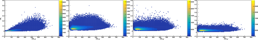
Figure 23: 2D Histogram of jet mass vs autoencoder loss for the four cases mentioned in the text: preprocessing without Lorentz boost + Arch-1 (first from left), preprocessing without using Gram-Schmidt axis + Arch-1 (second), full preprocessing + Arch-1 (third), and finally, full preprocessing + Arch-3 (fourth).

Appendix C The Convolutional Autoencoder

Here, we give a the pseudo-code describing the convolutional autoencoder (Arch-3):

ΨConv2D(channels=50,kernel_size=5,activation=’relu’)
ΨMaxPool2D(pool_size=2, strides=2)
ΨConv2D(channels=50,kernel_size=5,activation=’relu’)
ΨMaxPool2D(pool_size=2, strides=2)
ΨConv2D(channels=50,kernel_size=5,activation=’relu’)
ΨFlatten()
ΨDense(100,activation="relu")
ΨDense(450,activation="relu")
Ψreshape(50,3,3)
ΨConv2DTranspose(channels=50,kernel_size=9,stride=2,padding=0,activation="relu")
ΨConv2DTranspose(channels=50,kernel_size=9,stride=2,padding=0,activation="relu")
ΨConv2DTranspose(channels=1,kernel_size=8,stride=1,padding=0,activation="relu")
ΨFlatten()
Ψsoftmax()
Ψreshape(1,40,40)
Ψ

Appendix D Details of training

We have used 2400000 QCD-jet images for training and 400000 QCD-jet images for testing. We generally trained for 20 epochs, since as can be seen in Figure 24, there is no significant difference in the loss per epoch even if one goes beyond 20.

Figure 24: The variation of training and testing loss curves with number of training epochs for the CNN autoencoder (Arch-3)

Figure 25: The distributions of $m_{J}$ in bins of $\epsilon$ for QCD-jets using the training (left) and testing (middle) datasets, as well as the distributions of $\epsilon$ (right), when we use the convolutional autoencoder from Arch-3.

We consider additional checks to make sure that we do not over-train. For example, we provide comparison plots for training and testing datasets in Figure 25. Clearly, the difference between the distributions for training and testing are generally negligible.

Appendix E The choice of $m_{0}/E_{0}$

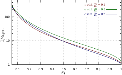
Figure 26: A comparison of QCD vs top jet discrimination ROC (using only the autoencoder loss) for the 3 cases of $\frac{m_{0}}{E_{0}}=0.1$, $\frac{m_{0}}{E_{0}}=0.5$ and $\frac{m_{0}}{E_{0}}=0.7$ for the shallow dense network (Arch-2).

Throughout this work we use $m_{0}=0.5~{}\text{GeV}$ and $E_{0}=1~{}\text{GeV}$, in order to prepare jet images. One expects that the information content in these images and, therefore, the performances of auto-encoders to be sensitive on the choice of $m_{0}$ and $E_{0}$, or rather on the ratio $m_{0}/E_{0}$. Clearly, one does not take arbitrary $m_{0}/E_{0}$ and expects to get identical performance. A tiny $m_{0}/E_{0}$ implies that the most energetic components of the final boosted jet occupy a narrow cone inside the jet, and get mapped to a few pixels at the center of the image by construction. Similarly, a large $m_{0}/E_{0}$, sends all energetic particles to the periphery. In both these extreme limits, a large number of constituents may get mapped to the same pixels, and consequently the image looses substructure information of the jet.

We demonstrate how the performance of the auto-encoder changes as we vary $m_{0}/E_{0}$ in Figure 26. Here we compare ROC curves for QCD-jets vs top jet discrimination. The red, green, and blue lines in Figure 26 represent performances when images are produced using $m_{0}/E_{0}$ to be $0.1$, $0.5$ and $0.7$ respectively. As can be seen in the figure, the change in performance is rather reasonable. For the same background efficiency, we see that the signal efficiency varies by order $10\%$, even when we change $m_{0}/E_{0}$ by order $40\%$ or more around $m_{0}/E_{0}=0.5$ (the operating point in this work).

Appendix F Benchmarking auto-encoder loss for supervised learning with standard dataset

In Section 3.3.1 we suggested that the loss function $\epsilon$ can be used in a supervised manner as well. It is tempting to benchmark this performances with respect to the garden variety of supervised algorithms available. Of course, the exact dataset one uses to draw comparisons always provides grounds for contentions. In order to mitigate these concerns, we provide the plot in Figure 27, where we repeat our analyses using the data sample used in Ref. Kasieczka:2019dbj . For this analysis, we do not perform any new optimization but just use the Arch-2 model that was already described. In this plot, the solid curves represent the result of our analyses. One of the advantage of using the same dataset as in Ref. Kasieczka:2019dbj , implies that we can readily compare these performances with the stack of ROCs (using an ensemble of supervised learners) given in Ref. Kasieczka:2019dbj . For the sake of reference, we also show the ROC for supervised learning using ParticleNet, as reported in Ref. Kasieczka:2019dbj . As clearly demonstrated in Figure 27, the discrimination performance of a BDT (to separate top-jets from QCD-jets) which combines high level jet observables like the auto-encoder loss, jet-mass, and $N$-subjettiness variables compares favorable well to the performance of the ‘‘state-of-the-art" supervised algorithms from Ref. Kasieczka:2019dbj .

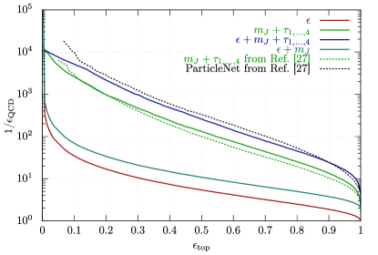
Figure 27: ROC for QCD vs top jet discrimination compared with results from Ref. Kasieczka:2019dbj .

References

- (1) CMS Collaboration Collaboration, S. Chatrchyan et al., ‘‘Observation of a new boson at a mass of 125 GeV with the CMS experiment at the LHC,’’ Phys.Lett. B716 (2012) 30–61, arXiv:1207.7235 [hep-ex]. https://arxiv.org/abs/1207.7235.
- (2) ATLAS Collaboration Collaboration, G. Aad et al., ‘‘Observation of a new particle in the search for the Standard Model Higgs boson with the ATLAS detector at the LHC,’’ Phys.Lett. B716 (2012) 1–29, arXiv:1207.7214 [hep-ex]. https://arxiv.org/abs/1207.7214.
- (3) J. M. Butterworth, A. R. Davison, M. Rubin, and G. P. Salam, ‘‘Jet substructure as a new Higgs search channel at the LHC,’’ Phys. Rev. Lett. 100 (2008) 242001, arXiv:0802.2470 [hep-ph].
- (4) G. P. Salam, ‘‘Towards Jetography,’’ Eur. Phys. J. C67 (2010) 637--686, arXiv:0906.1833 [hep-ph].
- (5) D. Krohn, J. Thaler, and L.-T. Wang, ‘‘Jet Trimming,’’ JHEP 02 (2010) 084, arXiv:0912.1342 [hep-ph].
- (6) S. D. Ellis, C. K. Vermilion, and J. R. Walsh, ‘‘Recombination Algorithms and Jet Substructure: Pruning as a Tool for Heavy Particle Searches,’’ Phys. Rev. D81 (2010) 094023, arXiv:0912.0033 [hep-ph].
- (7) A. Chakraborty, A. M. Iyer, and T. S. Roy, ‘‘A Framework for Finding Anomalous Objects at the LHC,’’ Nucl. Phys. B932 (2018) 439--470, arXiv:1707.07084 [hep-ph].
- (8) J. A. Aguilar-Saavedra, J. H. Collins, and R. K. Mishra, ‘‘A generic anti-QCD jet tagger,’’ JHEP 11 (2017) 163, arXiv:1709.01087 [hep-ph].
- (9) T. Cohen, M. Freytsis, and B. Ostdiek, ‘‘(Machine) Learning to Do More with Less,’’ JHEP 02 (2018) 034, arXiv:1706.09451 [hep-ph].
- (10) H. Qu and L. Gouskos, ‘‘ParticleNet: Jet Tagging via Particle Clouds,’’ arXiv:1902.08570 [hep-ph].
- (11) K. Datta and A. Larkoski, ‘‘How Much Information is in a Jet?,’’ JHEP 06 (2017) 073, arXiv:1704.08249 [hep-ph].
- (12) L. Moore, K. Nordström, S. Varma, and M. Fairbairn, ‘‘Reports of My Demise Are Greatly Exaggerated: -subjettiness Taggers Take On Jet Images,’’ arXiv:1807.04769 [hep-ph].
- (13) P. T. Komiske, E. M. Metodiev, and J. Thaler, ‘‘Energy Flow Networks: Deep Sets for Particle Jets,’’ JHEP 01 (2019) 121, arXiv:1810.05165 [hep-ph].
- (14) A. Butter, G. Kasieczka, T. Plehn, and M. Russell, ‘‘Deep-learned Top Tagging with a Lorentz Layer,’’ SciPost Phys. 5 no. 3, (2018) 028, arXiv:1707.08966 [hep-ph].
- (15) P. T. Komiske, E. M. Metodiev, and J. Thaler, ‘‘Energy flow polynomials: A complete linear basis for jet substructure,’’ JHEP 04 (2018) 013, arXiv:1712.07124 [hep-ph].
- (16) G. Louppe, K. Cho, C. Becot, and K. Cranmer, ‘‘QCD-Aware Recursive Neural Networks for Jet Physics,’’ JHEP 01 (2019) 057, arXiv:1702.00748 [hep-ph].
- (17) M. Erdmann, E. Geiser, Y. Rath, and M. Rieger, ‘‘Lorentz Boost Networks: Autonomous Physics-Inspired Feature Engineering,’’ arXiv:1812.09722 [hep-ex].
- (18) A. Hoecker, P. Speckmayer, J. Stelzer, J. Therhaag, E. von Toerne, and H. Voss, ‘‘TMVA: Toolkit for Multivariate Data Analysis,’’ PoS ACAT (2007) 040, arXiv:physics/0703039.
- (19) J. Pearkes, W. Fedorko, A. Lister, and C. Gay, ‘‘Jet Constituents for Deep Neural Network Based Top Quark Tagging,’’ arXiv:1704.02124 [hep-ex].
- (20) L. G. Almeida, M. Backović, M. Cliche, S. J. Lee, and M. Perelstein, ‘‘Playing Tag with ANN: Boosted Top Identification with Pattern Recognition,’’ JHEP 07 (2015) 086, arXiv:1501.05968 [hep-ph].
- (21) S. Macaluso and D. Shih, ‘‘Pulling Out All the Tops with Computer Vision and Deep Learning,’’ JHEP 10 (2018) 121, arXiv:1803.00107 [hep-ph].
- (22) G. Kasieczka, T. Plehn, M. Russell, and T. Schell, ‘‘Deep-learning Top Taggers or The End of QCD?,’’ JHEP 05 (2017) 006, arXiv:1701.08784 [hep-ph].
- (23) J. Cogan, M. Kagan, E. Strauss, and A. Schwarztman, ‘‘Jet-Images: Computer Vision Inspired Techniques for Jet Tagging,’’ JHEP 02 (2015) 118, arXiv:1407.5675 [hep-ph].
- (24) P. Baldi, K. Bauer, C. Eng, P. Sadowski, and D. Whiteson, ‘‘Jet Substructure Classification in High-Energy Physics with Deep Neural Networks,’’ Phys. Rev. D93 no. 9, (2016) 094034, arXiv:1603.09349 [hep-ex].
- (25) L. de Oliveira, M. Kagan, L. Mackey, B. Nachman, and A. Schwartzman, ‘‘Jet-images — deep learning edition,’’ JHEP 07 (2016) 069, arXiv:1511.05190 [hep-ph].
- (26) J. H. Collins, K. Howe, and B. Nachman, ‘‘Extending the search for new resonances with machine learning,’’ Phys. Rev. D99 no. 1, (2019) 014038, arXiv:1902.02634 [hep-ph].
- (27) A. Butter et al., ‘‘The Machine Learning Landscape of Top Taggers,’’ arXiv:1902.09914 [hep-ph].
- (28) J. H. Collins, K. Howe, and B. Nachman, ‘‘Anomaly Detection for Resonant New Physics with Machine Learning,’’ Phys. Rev. Lett. 121 no. 24, (2018) 241803, arXiv:1805.02664 [hep-ph].
- (29) O. Cerri, T. Q. Nguyen, M. Pierini, M. Spiropulu, and J.-R. Vlimant, ‘‘Variational Autoencoders for New Physics Mining at the Large Hadron Collider,’’ arXiv:1811.10276 [hep-ex].
- (30) A. Andreassen, I. Feige, C. Frye, and M. D. Schwartz, ‘‘JUNIPR: a Framework for Unsupervised Machine Learning in Particle Physics,’’ Eur. Phys. J. C79 no. 2, (2019) 102, arXiv:1804.09720 [hep-ph].
- (31) M. Farina, Y. Nakai, and D. Shih, ‘‘Searching for New Physics with Deep Autoencoders,’’ arXiv:1808.08992 [hep-ph].
- (32) T. Heimel, G. Kasieczka, T. Plehn, and J. M. Thompson, ‘‘QCD or What?,’’ arXiv:1808.08979 [hep-ph].
- (33) J. Hajer, Y.-Y. Li, T. Liu, and H. Wang, ‘‘Novelty Detection Meets Collider Physics,’’ arXiv:1807.10261 [hep-ph].
- (34) M. Dasgupta, A. Fregoso, S. Marzani, and G. P. Salam, ‘‘Towards an understanding of jet substructure,’’ JHEP 09 (2013) 029, arXiv:1307.0007 [hep-ph].
- (35) T. Plehn and M. Spannowsky, ‘‘Top Tagging,’’ J. Phys. G39 (2012) 083001, arXiv:1112.4441 [hep-ph].
- (36) G. Kasieczka, T. Plehn, T. Schell, T. Strebler, and G. P. Salam, ‘‘Resonance Searches with an Updated Top Tagger,’’ JHEP 06 (2015) 203, arXiv:1503.05921 [hep-ph].
- (37) T. Plehn, M. Spannowsky, M. Takeuchi, and D. Zerwas, ‘‘Stop Reconstruction with Tagged Tops,’’ JHEP 10 (2010) 078, arXiv:1006.2833 [hep-ph].
- (38) T. Plehn, G. P. Salam, and M. Spannowsky, ‘‘Fat Jets for a Light Higgs,’’ Phys. Rev. Lett. 104 (2010) 111801, arXiv:0910.5472 [hep-ph].
- (39) G. F. Sterman, ‘‘Some Basic Concepts of Perturbative QCD,’’ Acta Phys. Polon. B39 (2008) 2151--2172, arXiv:0807.5118 [hep-ph].
- (40) M. Cacciari, G. P. Salam, and G. Soyez, ‘‘The anti- jet clustering algorithm,’’ JHEP 04 (2008) 063, arXiv:0802.1189 [hep-ph].
- (41) Y. L. Dokshitzer, G. D. Leder, S. Moretti, and B. R. Webber, ‘‘Better jet clustering algorithms,’’ JHEP 08 (1997) 001, arXiv:hep-ph/9707323 [hep-ph].
- (42) S. D. Ellis and D. E. Soper, ‘‘Successive combination jet algorithm for hadron collisions,’’ Phys. Rev. D48 (1993) 3160--3166, arXiv:hep-ph/9305266 [hep-ph].
- (43) S. Catani, Y. L. Dokshitzer, M. H. Seymour, and B. R. Webber, ‘‘Longitudinally invariant clustering algorithms for hadron hadron collisions,’’ Nucl. Phys. B406 (1993) 187--224.
- (44) G. C. Blazey et al., ‘‘Run II jet physics,’’ in QCD and weak boson physics in Run II. Proceedings, Batavia, USA, March 4-6, June 3-4, November 4-6, 1999, pp. 47--77. 2000. arXiv:hep-ex/0005012 [hep-ex]. http://lss.fnal.gov/cgi-bin/find_paper.pl?conf-00-092.
- (45) M. Cacciari, G. P. Salam, and G. Soyez, ‘‘Fastjet user manual,’’ The European Physical Journal C 72 no. 3, (Mar, 2012) 1896. https://doi.org/10.1140/epjc/s10052-012-1896-2.
- (46) A. Zucconi, ‘‘AN INTRODUCTION TO AUTOENCODERS.’’ https://www.alanzucconi.com/2018/03/14/an-introduction-to-autoencoders/.
- (47) Y. Lecun, L. Bottou, Y. Bengio, and P. Haffner, ‘‘Gradient-based learning applied to document recognition,’’ Proceedings of the IEEE 86 no. 11, (Nov, 1998) 2278--2324.
- (48) J. Masci, U. Meier, D. C. Ciresan, and J. Schmidhuber, ‘‘Stacked Convolutional Auto-Encoders for Hierarchical Feature Extraction,’’ in 21st International Conference on Artificial Neural Networks, Espoo, Finland, June 14-17, 2011, Proceedings, Part I, T. Honkela, W. Duch, M. Girolami, and S. Kaski, eds., International Conference on Artificial Neural Networks (ICANN). 2011.
- (49) Hahnloser Richard H. R., Sarpeshkar Rahul, Mahowald Misha A., Douglas Rodney J., and Seung H. Sebastian, ‘‘Digital selection and analogue amplification coexist in a cortex-inspired silicon circuit,’’ Nature 405 (Jun, 2000) 947. https://www.nature.com/articles/35016072#supplementary-information.
- (50) D. P. Kingma and M. Welling, ‘‘Auto-Encoding Variational Bayes,’’ arXiv e-prints (Dec., 2013) arXiv:1312.6114, arXiv:1312.6114 [stat.ML].
- (51) L. Mescheder, S. Nowozin, and A. Geiger, ‘‘Adversarial Variational Bayes: Unifying Variational Autoencoders and Generative Adversarial Networks,’’ arXiv e-prints (Jan, 2017) arXiv:1701.04722, arXiv:1701.04722 [cs.LG].
- (52) R. Prescott Adams and R. S. Zemel, ‘‘Ranking via Sinkhorn Propagation,’’ arXiv e-prints (June, 2011) arXiv:1106.1925, arXiv:1106.1925 [stat.ML].
- (53) J. W. Monk, ‘‘Deep Learning as a Parton Shower,’’ arXiv:1807.03685 [hep-ph].
- (54) T. Sjostrand, S. Mrenna, and P. Z. Skands, ‘‘PYTHIA 6.4 Physics and Manual,’’ JHEP 05 (2006) 026, arXiv:hep-ph/0603175 [hep-ph].
- (55) T. Sjöstrand, S. Ask, J. R. Christiansen, R. Corke, N. Desai, P. Ilten, S. Mrenna, S. Prestel, C. O. Rasmussen, and P. Z. Skands, ‘‘An Introduction to PYTHIA 8.2’’ Comput. Phys. Commun. 191 (2015) 159--177, arXiv:1410.3012 [hep-ph].
- (56) DELPHES 3 Collaboration, J. de Favereau, C. Delaere, P. Demin, A. Giammanco, V. Lemaître, A. Mertens, and M. Selvaggi, ‘‘DELPHES 3, A modular framework for fast simulation of a generic collider experiment,’’ JHEP 02 (2014) 057, arXiv:1307.6346 [hep-ex].
- (57) D. P. Kingma and J. Ba, ‘‘Adam: A method for stochastic optimization,’’ CoRR abs/1412.6980 (2014) , arXiv:1412.6980. http://arxiv.org/abs/1412.6980.
- (58) T. Chen, M. Li, Y. Li, M. Lin, N. Wang, M. Wang, T. Xiao, B. Xu, C. Zhang, and Z. Zhang, ‘‘MXNet: A Flexible and Efficient Machine Learning Library for Heterogeneous Distributed Systems,’’ arXiv e-prints (Dec., 2015) arXiv:1512.01274, arXiv:1512.01274 [cs.DC].
- (59) M. Abadi, A. Agarwal, P. Barham, E. Brevdo, Z. Chen, C. Citro, G. S. Corrado, A. Davis, J. Dean, M. Devin, S. Ghemawat, I. J. Goodfellow, A. Harp, G. Irving, M. Isard, Y. Jia, R. Józefowicz, L. Kaiser, M. Kudlur, J. Levenberg, D. Mané, R. Monga, S. Moore, D. G. Murray, C. Olah, M. Schuster, J. Shlens, B. Steiner, I. Sutskever, K. Talwar, P. A. Tucker, V. Vanhoucke, V. Vasudevan, F. B. Viégas, O. Vinyals, P. Warden, M. Wattenberg, M. Wicke, Y. Yu, and X. Zheng, ‘‘Tensorflow: Large-scale machine learning on heterogeneous distributed systems,’’ CoRR abs/1603.04467 (2016) , arXiv:1603.04467. http://arxiv.org/abs/1603.04467.
- (60) Y. Tang, ‘‘Tf.learn: Tensorflow’s high-level module for distributed machine learning,’’ CoRR abs/1612.04251 (2016) , arXiv:1612.04251. http://arxiv.org/abs/1612.04251.
- (61) J. Gallicchio and M. D. Schwartz, ‘‘Seeing in Color: Jet Superstructure,’’ Phys. Rev. Lett. 105 (2010) 022001, arXiv:1001.5027 [hep-ph].
- (62) M. Dasgupta, M. Guzzi, J. Rawling, and G. Soyez, ‘‘Top tagging : an analytical perspective,’’ JHEP 09 (2018) 170, arXiv:1807.04767 [hep-ph].
- (63) M. Dasgupta, A. Fregoso, S. Marzani, and A. Powling, ‘‘Jet substructure with analytical methods,’’ Eur. Phys. J. C73 no. 11, (2013) 2623, arXiv:1307.0013 [hep-ph].
- (64) S. Marzani, G. Soyez, and M. Spannowsky, ‘‘Looking inside jets: an introduction to jet substructure and boosted-object phenomenology,’’ arXiv:1901.10342 [hep-ph].
- (65) D. E. Kaplan, K. Rehermann, M. D. Schwartz, and B. Tweedie, ‘‘Top Tagging: A Method for Identifying Boosted Hadronically Decaying Top Quarks,’’ Phys. Rev. Lett. 101 (2008) 142001, arXiv:0806.0848 [hep-ph].
- (66) J. Thaler and K. Van Tilburg, ‘‘Maximizing Boosted Top Identification by Minimizing N-subjettiness,’’ JHEP 02 (2012) 093, arXiv:1108.2701 [hep-ph].
- (67) CMS Collaboration, C. Collaboration, ‘‘Boosted Top Jet Tagging at CMS,’’.
- (68) ATLAS Collaboration, M. Aaboud et al., ‘‘Performance of top-quark and -boson tagging with ATLAS in Run 2 of the LHC,’’ arXiv:1808.07858 [hep-ex].
- (69) R. Brun and F. Rademakers, ‘‘Root — an object oriented data analysis framework,’’ Nuclear Instruments and Methods in Physics Research Section A: Accelerators, Spectrometers, Detectors and Associated Equipment 389 no. 1, (1997) 81 -- 86. http://www.sciencedirect.com/science/article/pii/S016890029700048X. New Computing Techniques in Physics Research V.
- (70) S. D. Ellis, A. Hornig, D. Krohn, and T. S. Roy, ‘‘On Statistical Aspects of Qjets,’’ JHEP 01 (2015) 022, arXiv:1409.6785 [hep-ph].
- (71) S. D. Ellis, A. Hornig, T. S. Roy, D. Krohn, and M. D. Schwartz, ‘‘Qjets: A Non-Deterministic Approach to Tree-Based Jet Substructure,’’ Phys. Rev. Lett. 108 (2012) 182003, arXiv:1201.1914 [hep-ph].
- (72) A. J. Larkoski, G. P. Salam, and J. Thaler, ‘‘Energy Correlation Functions for Jet Substructure,’’ JHEP 06 (2013) 108, arXiv:1305.0007 [hep-ph].
- (73) I. W. Stewart, F. J. Tackmann, and W. J. Waalewijn, ‘‘N-Jettiness: An Inclusive Event Shape to Veto Jets,’’ Phys. Rev. Lett. 105 (2010) 092002, arXiv:1004.2489 [hep-ph].
- (74) J. Thaler and K. Van Tilburg, ‘‘Identifying Boosted Objects with N-subjettiness,’’ JHEP 03 (2011) 015, arXiv:1011.2268 [hep-ph].
- (75) CMS Collaboration, V. Khachatryan et al., ‘‘Identification techniques for highly boosted W bosons that decay into hadrons,’’ JHEP 12 (2014) 017, arXiv:1410.4227 [hep-ex].
- (76) D. Krohn, M. D. Schwartz, M. Low, and L.-T. Wang, ‘‘Jet Cleansing: Pileup Removal at High Luminosity,’’ Phys. Rev. D90 no. 6, (2014) 065020, arXiv:1309.4777 [hep-ph].
- (77) M. Cacciari, G. P. Salam, and G. Soyez, ‘‘SoftKiller, a particle-level pileup removal method,’’ Eur. Phys. J. C75 no. 2, (2015) 59, arXiv:1407.0408 [hep-ph].
- (78) D. Bertolini, P. Harris, M. Low, and N. Tran, ‘‘Pileup Per Particle Identification,’’ JHEP 10 (2014) 059, arXiv:1407.6013 [hep-ph].
- (79) P. T. Komiske, E. M. Metodiev, B. Nachman, and M. D. Schwartz, ‘‘Pileup Mitigation with Machine Learning (PUMML),’’ JHEP 12 (2017) 051, arXiv:1707.08600 [hep-ph].