A code for robust astrometric solution of astronomical images
Abstract
I present a software tool for solving the astrometry of astronomical images. The code puts emphasis on robustness against failures for correctly matching the sources in the image to a reference catalog, and on the stability of the solutions over the field of view (e.g., using orthogonal polynomials for the fitted transformation). The code was tested on over images from various sources, including the Palomar Transient Factory (PTF) and the Zwicky Transient Facility (ZTF). The tested images equally represent low and high Galactic latitude fields and exhibit failure/bad-solution rate of . Running on PTF 60-s integration images, and using the GAIA-DR2 as a reference catalog, the typical two-axes-combined astrometric root-mean square (RMS) is 14 mas at the bright end, presumably due to astrometric scintillation noise and systematic errors. I discuss the effects of seeing, airmass and the order of the transformation on the astrometric accuracy. The software, available online, is developed in MATLAB as part of an astronomical image processing environment and it can be run also as a stand-alone code.
Subject headings:
techniques: image processing – methods: data analysis1. Introduction
There is a large variety of existing software for astrometric solutions (e.g., SCamp, Bertin 2006, 2010; Astrometry.net, Lang et al. 2010, 2012; ASCfit, Jørgensen et al. 2002, Pickles 2012). Some of these tools are extremely powerful. For example, astrometry.net is capable of matching star patterns in an image-catalog to a reference-catalog, without prior knowledge on the image’s sky position, rotation or scale. This feature is valuable, for example, when solving the astrometry of ancient photographic plates for which the plate scale, rotation and sky location is errornous or unavailable (e.g., Tang et al. 2013). However, in some cases, the approximate sky position, plate scale and rotation are known, and simpler, quicker and more robust approaches can be used (e.g., Bertin 2006).
Here I present a software tool for solving the astrometry of astronomical images, particularly wide-field and dense fields. This code attempts to improve over some existing tools in one aspect, which is robustness against failures and inaccurate solutions. My main motivation was based on the Palomar Transient Factory (PTF; Law et al. 2009; Rau et al. 2009) pipeline (Laher et al. 2014), which uses SCamp (Bertin 2006) and Astrometry.net (Lang et al. 2010). A total of about 4% of the PTF images are reported to have poor astrometric solutions (see Laher et al. 2014), and this fraction can reach about 30% in some fields near the Galactic plane. In many cases, this is due to anomalous distortion coefficients, or poor solutions in some parts of the image. We identify two main problems: The first issue is that in some cases the correct solution cannot be found. This may happen, for example, in fields with high stellar density, or in large field-of-view images taken at high airmass, which causes the plate scale to be position-dependent. The second issue is that, sometimes, fitting a high order polynomial transformation returns an adequate solution in some region of the field but provides a poor fit in other regions. This specific problem may happen, for example, when the fitted transformation is ill-conditioned.
Our strategy to mitigate these two problems is relatively straightforward. The solution consists of two minor modifications to the typical approach, which can be implemented in other tools. The first improvement is to divide the image into several smaller sub-images, and then attempt to mach the stars to the catalog sources in each sub-image separately. In this case it is easy to identify and reject bad solutions (i.e., a solution that is different from the solutions of the other sub images). Moreover, the good solutions can be used to interpolate over the regions with bad solutions. The second strategy is to use orthogonal polynomials for the transformation, or transformations that have a physical motivation (e.g., tip-tilt transformation). A feature of the current version of the code over, e.g., Astrometry.net, is that it requires rough knowledge of the image coordinates and plate scale and hence needs to be configured for each telescope/instrument on which it is used.
2. General description of the code
The algorithm starts with either the image or catalog of sources in the image. If the image is provided without a catalog, the code finds the sources in the image and measures their X/Y positions and instrumental magnitudes using mextractor (Ofek et al. in prep) or SExtractor (Bertin & Arnouts 1996). The code can use a mask image, and a bitmask-dictionary111A mask-dictionary relates a problem to a bit-index., that indicate problems per pixel in the input image. The mask image can be used to remove sources that may badly affect the solution (e.g., cosmic rays, saturated pixels). Furthermore, the code can remove sources based on a surface density criteria. This is done by identifying regions with a large number of sources per unit area, and rows/columns in which the number of sources is above the mean source row/column density. This step is important as very high density regions can sometimes be matched with a wrong solution. The user supplies the code with approximate image coordinates, radius in which the reference catalog sources are extracted222Due to uncertainties in the image position, the catalog search radius can be larger than the image size, possible coordinate flips, plate scale, and, optionally, the range of the image rotation (i.e., the position angle of the Y-axis).
Next, the code extracts the stars from the reference catalog according to user- or header-specified approximate coordinates. The code can access a large number of online reference catalogs (e.g., VizieR, Ochsenbein et al. 2000), user-supplied catalogs, or local catalogs in the catsHTM format (Soumagnac & Ofek 2018) that provide fast access to large catalogs. If the reference catalog includes proper motions (and, optionally, parallaxes and radial velocities), the coordinates are transformed to the image-catalog epoch. The catalog coordinates are then projected onto a plane using the gnomonic (tangential) projection (e.g., Calabretta & Greisen 2002) and the known image plate scale. If needed, the code may equalize the source surface density in the image catalog and reference catalog by removing the faintest sources in the image-catalog or reference-catalog – whichever contains more sources per unit area.
Next, the code attempts to match the sources in the image catalog to the projected reference-catalog sources. The image catalog is partitioned into sub catalogs of smaller regions of the image (i.e., sub-images with default size of pixels), and the matching process is done separately for each region. This step is designed to make the code robust against plate-scale changes as a function of position and to deal with failures to match the catalogs – i.e., it increases the probability that at least some of the stars in the field will be matched to the reference catalog. By default, the code first attempts to find possible rotational solutions using the algorithm suggested by Kaiser et al. (1999) and used in SCamp (Bertin 2006). This is done by calculating the distances and position angles between all the pairs of sources in the image catalog, and all the pairs of sources in the reference catalog. Next, a two dimensional histogram of distance and position angle is generated for each catalog, and the two histograms are cross-correlated to find possible rotations between the image catalog and reference catalog. Alternatively, if this step fails or the user chooses to skip this step, the code can look for possible shifts, between the catalogs, for a range of possible rotations specified by the user.
Following the algorithm implemented by Giveon et al. (1999), for each possible rotation and coordinate flip, the code calculates all the possible shifts in X and Y coordinates between the sources in the image and the projected sources in the reference catalog. A two-dimensional histogram (in X and Y) of all the possible differences is calculated and peaks in the histogram are identified. By default, the code does not select just the highest peak in each histogram, rather, it includes all the peaks satisfying some user-specified criteria (e.g., signal-to-noise ratio). The result is that the code collects many possible solutions with different rotations, flips, and shifts. Next, each one of the possible solutions is tested. This is done, for each candidate solution, by fitting an affine transformation between the image catalog sources and reference catalog sources. For each transformation, the root-mean square (RMS) of residuals and the number of matched stars are reported, and the best solution is selected based on some user-specified criteria (e.g., RMS and/or number of matched stars).
The code compares the solutions of the various sub-images and reject sub-images with solutions which are different than the median solution. Therefore, this step may result in sub-images without matched stars. The code uses the matched stars over all sub-images to fit a general transformation between the image catalog and reference catalog. The available transformations include affine transformation, tip-tilt terms (e.g., , where and are free parameters; van Altena 2012), general polynomials, and orthogonal Chebyshev polynomials. The default transformation depends on the number of matched sources. The fit includes iterative removal of outliers. The default is to use two iterations with sigma clipping of - after the first iteration. In the second iteration a weighted fitting is implemented, where the weights are the inverse variance. Here, the variances are obtained from the RMS as a function of magnitude plot of the first-iteration fit. Note that a more aggressive sigma-clipping may lead, in some cases, to the rejection of good reference stars and bias in the estimated transformation.
The transformation parameters are converted into a polynomial representation and added to the image header in the TPV World Coordinate System representation333https://fits.gsfc.nasa.gov/registry/tpvwcs/tpv.html (see also Calabretta & Greisen 2002).
3. Performances
I tested the code on over 50,000 images from various sources. The main data set used is from the Palomar Transient Factory (PTF; Law et al. 2009; Rau et al. 2009). The code was also tested on images from the Zwicky Transient Facility (Bellm et al. 2018), the Palomar WIRC infrared camera, and the 28′′ telescope at the Wise observatory. The PTF data reduction is described in Laher et al. (2014) and Ofek et al. (2012). Each PTF image444The PTF camera has 11 active CCDs and we refer to the data from each CCD as an image. is 20484096 pixels, with a pix-1 scale. The ZTF data reduction pipeline is described in Masci et al. (2018). The ZTF images555The ZTF camera has 16 CCDs, each with four amplifiers. The data from each amplifier is treated as an individual image. are 30803072 pixels, with the same pixel scale as in the PTF images.
Testing the code on over 50,000 images, I encountered zero failures. Here failure is defined as either inability to find a solution, or solutions with large RMS in some regions of the image (see details below). In cases in which the number of matched stars was low (sometimes indicative of a problem), I inspected the images by eye and verified the solution was correct.
Below I present the statistics of the results from a homogeneous dataset of 8,548 PTF images. The images in this dataset were selected randomally by sky position, so a large fraction of the images were at low Galactic latitudes.
For the reference catalog, as a default, I used the GAIA-DR2 catalog (Gaia Collaboration, et al. 2018). However, the code was also tested using the GAIA-DR1 catalog (Gaia Collaboration, et al. 2016) and the UCAC-4 catalog (Zacharias et al. 2013). For the transformation between the reference catalog and the image-catalog, the code fitted an affine transformation plus a 4th order Chebyshev polynomial of the second kind. In the fitting procedure, two iterations were performed. Before the second iteration the code removed sources using a 5- clipping, where the standard deviation, , was calculated as a function of magnitude. Sources were extracted from the images using mextractor (Ofek et al. in prep.). I also tested the code on source catalogs generated using SExtractor (Bertin & Arnouts 1996) and DAOPHOT (Stetson 1987). Specifically, the DAOPHOT catalogs were generated by the PTF pipeline. However, for the DAOPHOT catalogs, I encountered failures in about 1% of the cases, due to some issues with the PTF-generated catalogs. Problems included invalid magnitudes and errors in the Point-Spread Function (PSF) extraction.
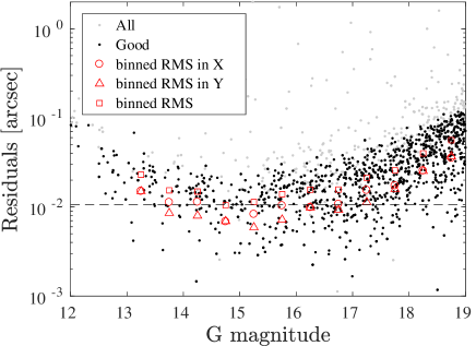
Figure 1 shows the residuals (square root of sum of squares of and residuals) as a function of the GAIA magnitude. This is shown for the first image in the dataset. The minimum RMS, of about 11 mas, is achieved for the brightest non-saturated stars (i.e., magnitude ). Unless explictly indicated, all rms values are for the two-axes combined rms. The single-axis rms is typically times smaller than the two-axes combined rms.

At the bright end of the non saturated stars, the solution is presumably limited by atmospheric scintillation noise and systematic errors, while at the faint-end, the solution degrades and is limited by Poisson noise. To characterize the quality of the astrometric solution we are interested in a metric which does not depend on the magnitude-range of stars used in the solution. Therefore, the adopted estimator for the quality of the solution is the RMS at the bright end for unsaturated stars. For ground based, seeing-limited observations, the RMS measured at the minimum of the magnitude-RMS plot, is typically dominated by the scintillation noise and any additional systematic errors. For this reason, I define the asymptotic RMS as the minimum RMS of a second-order polynomial fitted to the RMS vs. magnitude plot, in the range of available stellar magnitudes above the saturation limit. The dashed line in Figure 1 represents the level of the measured asymptotic RMS for this case. Note that, unless indicated explicitly, all the RMS values used are simple standard deviations, and not robust estimators.
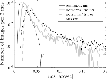
Figure 2 shows the distribution of RMS measurements over the sample of PTF images. The solid black line represents the asymptotic RMS. This curve peaks at 13.8 mas, and its lower and upper 5-percentile are at 8.9 mas and 38.9 mas, respectively. The worst asymptotic RMS I encountered in this sample is 89 mas. On closer inspection of the four images with asymptotic RMS larger than mas, I found that three of them have poor seeing () and the fourth has a double-peaked PSF due to a tracking problem.

The solid gray line presents the total robust RMS of all the stars used in the solution (i.e., not only the bright stars). As expected, due to the Poisson noise, it has a longer tail. Also shown as dashed gray line, is the robust RMS of all the matched stars in the image (i.e., before the sigma clipping).
The solutions of the ZTF images have RMS values that are about larger than those in the PTF images. This is presumably due the fact that the ZTF integration time is half of the PTF exposure times, and that the astrometric scintillation noise decreases like the square root of the integration time (e.g., Shao & Colavita 1992).
An important test is to verify that the solution is good over the entire image. In order to test this, the code reports the number of matches and RMS in each sub-image of default size of pixels. Figure 3 presents a histogram of the number of images in which, 0, 1, 2, and 3 blocks (i.e., pix sub images in each image) have zero matched stars. I found that 49 images had one -pixels sub-image with zero matches, three images had two sub-images with zero matches, and one image had three sub-images with zero matches.

Zero matches in a small sub-image typically happens when the total number of stars in the image is low and/or in regions with elevated background. I inspected by eye all the cases with more than one sub-image with zero matches to verify the solutions are correct.
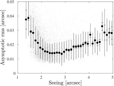
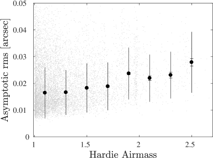
Another important property, which is relevant for all astrometric solvers, is the dependence of the quality of the solution on airmass and seeing. Figure 4 presents the asymptotic RMS as a function of the seeing. The gray points show the individual measurements, while the black circles indicate the median asymptotic RMS in seeing-bins. The full error bars represent the scatter of the points in each bin as calculated using the standard deviation, while the horizontal bars indicate the errors on the mean as estimated by the standard deviation divided by the square root of the number of points in the bin. The plot shows a clear minimum in the RMS around a seeing of . The degradation in the quality of the solution below seeing of about is presumably due to under-sampling of the PSF. The PTF pixel scale is pix-1. Although the Nyquist sampling criterion is not well defined for a Gaussian PSF666The Fourier transform of a Gaussian is another Gaussian and, therefore, is not bandlimted. However, in practice, the information content in the edges of the Gaussian is small., it is roughly requires that the full width at half maximum (FWHM) of the PSF contain about two pixels. Therefore, when the seeing is better than , the accuracy at which the source position can be determined degrades. For seeing above , the RMS increases again. Fitting a power-law to the RMS vs. seeing, in the range of to yielded a power-law index of .


The best fit power-law between the RMS and airmass, shows that the RMS goes like the airmass to the power of . The degradation of astrometry with airmass is expected due to several reasons. First, the seeing depends on the airmass. Indeed, in these PTF images, the Spearman rank correlation between the airmass and the seeing is 0.16 (with a false alarm probability ). An additional reason is that the atmospheric color-dependent refraction increases with airmass, which will tend to increase the RMS as a function of airmass regardless of the seeing (see example in Zackay, Ofek, & Gal-Yam 2016).
I also tested the convergence of the astrometric accuracy as a function of the transformation order. For example, for one PTF image, I found that the asymptotic RMS was , , and for an affine transformation, an affine transformation plus tip/tilt terms, an affine transformation plus tip/tilt terms plus third-order Chebyshev polynomials of the second kind, and an affine transformation plus tip/tilt terms plus fourth-order Chebyshev polynomials of the second kind, respectively.
4. Code
The code is available777https://webhome.weizmann.ac.il/home/eofek/matlab/,888https://github.com/EranOfek/MAAT as part of the MATLAB Astronomy & Astrophysics Toolbox (Ofek 2014). The main input arguments of the code, as well as usage examples, are provided in the online documentation999https://webhome.weizmann.ac.il/home/eofek/matlab/doc/astrometry.html.
The code was developed using an object-oriented approach. Specifically, the images are stored in a container of astronomical images (SIM class101010https://webhome.weizmann.ac.il/home/eofek/matlab/doc/SIM.html). Each container (object) optionally contains a background, noise, weight and bit-mask images, as well as a PSF, source catalog and header information. Each method (i.e., a function that operates on a class), including the main code described here, may create, use, and update the associated metadata. For example, if one method populates the catalog field in the image object, another method can use it, or modify it. In this case, a single object represents many types of data associated with an image. One outcome is that the image is always associated with its metadata (e.g., mask, background, catalog), and the user does not need to be concerned with how to access and update the metadata. Another advantage is that the SIM object can be an array of images and their metadata stored in memory. This may alleviate the need for many time-consuming and unnecessary read/write-to-disk operations.
5. Summary
I present a new code for solving the astrometry of astronomical images. The main feature of the code is its robustness against failures, which I demonstrate on a large number of wide-field images. The RMS of the astrometric residuals, obtained using this code, are presumably close to the atmospheric scintillation limit. This robustness is mainly achived by three steps: (1) removing sources found in regions of high source density; (2) Partitioning the image to sub-images in which each region is solved autonomously, and than using all the sources found in sub-images with good solutions for a global fit; and (3) Using orthogonal polynomials.
As a future prospect, a possible method to further improve the astrometric solutions is to utilize the fact that the astrometric scintillation noise is highly correlated (at least on arcmin-scales; e.g., Shao & Colavita 1992) with a correlation function that drops like
| (1) |
where is the variance and is the angular distance. Using this correlation function for the covariance of the fitted transformation, along with higher order polynomials, has the potential to reduce the residuals. This approach may be especially important in high stellar density fields. Another important task is to reduce the systematic errors due to the instrument (e.g., variations in the detector pixel size). Additional planned improvements are adding color terms to the transformation, and trying to identify examples of failures and fixing the code to solve these cases.
References
- Bertin & Arnouts (1996) Bertin, E., & Arnouts, S. 1996, A&AS, 117, 393
- Bertin (2001) Bertin, E. 2001, Mining the Sky, 353
- Bertin (2006) Bertin, E. 2006, Astronomical Data Analysis Software and Systems XV, 351, 112
- Bertin (2010) Bertin, E. 2010, Astrophysics Source Code Library, 10068
- Calabretta & Greisen (2002) Calabretta, M. R., & Greisen, E. W. 2002, A&A, 395, 1077
- Calabretta et al. (2004) Calabretta, M. R., Valdes, F., Greisen, E. W., & Allen, S. L. 2004, Astronomical Data Analysis Software and Systems (ADASS) XIII, 314, 551
- Gaia Collaboration, et al. (2016) Gaia Collaboration, Prusti, T., de Bruijne, J. H. J., et al. 2016, A&A, 595, A1.
- Gaia Collaboration et al. (2018) Gaia Collaboration, Brown, A. G. A., Vallenari, A., et al. 2018, arXiv:1804.09365
- Giveon et al. (1999) Giveon, U., Maoz, D., Kaspi, S., Netzer, H., & Smith, P. S. 1999, MNRAS, 306, 637
- Jones et al. (2017) Jones, R. L., Slater, C. T., Moeyens, J., et al. 2017, arXiv:1711.10621
- Jørgensen et al. (2002) Jørgensen, P. S., Riis, T., Betto, M., & Pickles, A. 2002, Astronomical Data Analysis Software and Systems XI, 281, 207
- Kaiser et al. (1999) Kaiser, N., Wilson, G., Luppino, G., & Dahle, H. 1999, arXiv:astro-ph/9907229
- Lang et al. (2010) Lang, D., Hogg, D. W., Mierle, K., Blanton, M., & Roweis, S. 2010, AJ, 139, 1782
- Lang et al. (2012) Lang, D., Hogg, D. W., Mierle, K., Blanton, M., & Roweis, S. 2012, Astrophysics Source Code Library, ascl:1208.001
- Ochsenbein et al. (2000) Ochsenbein, F., Bauer, P., & Marcout, J. 2000, A&AS, 143, 23
- Peng et al. (2002) Peng, C. Y., Ho, L. C., Impey, C. D., & Rix, H.-W. 2002, AJ, 124, 266
- Pickles (2012) Pickles, A. 2012, Astrophysics Source Code Library, ascl:1204.016
- Schechter et al. (1993) Schechter, P. L., Mateo, M., & Saha, A. 1993, PASP, 105, 1342
- Shao & Colavita (1992) Shao, M., & Colavita, M. M. 1992, A&A, 262, 353
- Stetson (1987) Stetson, P. B. 1987, PASP, 99, 191
- Tang et al. (2013) Tang, S., Grindlay, J., Los, E., & Servillat, M. 2013, PASP, 125, 857
- Taylor (2005) Taylor, M. B. 2005, Astronomical Data Analysis Software and Systems XIV, 347, 29
- Tody (1986) Tody, D. 1986, Proc. SPIE, 627, 733
- Udalski (2003) Udalski, A. 2003, ACTAA, 53, 291
- van Altena (2012) van Altena, W. F. 2012, Astrometry for Astrophysics, by William F. van Altena, ’Astrometry for Astrophysics’, Cambridge, UK: Cambridge University Press, 2012, p. 290.
- van Dokkum (2001) van Dokkum, P. G. 2001, PASP, 113, 1420
- Walter (2015) Walter, C. W. 2015, Journal of Instrumentation, 10, C05015
- Zacharias et al. (2013) Zacharias, N., Finch, C. T., Girard, T. M., et al. 2013, AJ, 145, 44