Cosmic web anisotropy is the primary indicator of halo assembly bias
Abstract
The internal properties of dark matter haloes correlate with the large-scale halo clustering strength at fixed halo mass – an effect known as assembly bias – and are also strongly affected by the local, non-linear cosmic web. Characterising a halo’s local web environment by its tidal anisotropy at scales the halo radius, we demonstrate that these multi-scale correlations represent two distinct statistical links: one between the internal property and , and the other between and large-scale ( ) halo bias . We focus on scalar internal properties of haloes related to formation time (concentration ), shape (mass ellipsoid asphericity ), velocity dispersion structure (velocity ellipsoid asphericity and velocity anisotropy ) and angular momentum (dimensionless spin ) in the mass range . Using conditional correlation coefficients and other detailed tests, we show that the joint distribution of , and any of the internal properties is consistent with , at all but the largest masses. Thus, the assembly bias trends reflect the two fundamental correlations and . Our results are unaffected by the exclusion of haloes with recent major merger events or splashback objects, although the latter are distinguished by the fact that does not explain their assembly bias trends. The overarching importance of provides a new perspective on the nature of assembly bias of distinct haloes, with potential ramifications for incorporating realistic assembly bias effects into mock catalogs of future large-scale structure surveys and for detecting galaxy assembly bias.
keywords:
cosmology: theory, dark matter, large-scale structure of the Universe – methods: numerical1 Introduction
The physical connection between the growth and properties of gravitationally collapsed dark matter haloes and the cosmic web environment in which these haloes reside is an interesting and challenging problem in the study of hierarchical structure formation (White & Silk, 1979; Eisenstein & Loeb, 1995; Bond & Myers, 1996; Bond et al., 1996; Monaco, 1999; Sheth & Tormen, 1999). Although the basic statistical connection between the very large-scale density environment (or halo bias) and halo properties such as mass was already established several decades ago (Kaiser, 1984; Bardeen et al., 1986; Bond et al., 1991; Lacey & Cole, 1993), subsequent technological improvements in simulating cold, collisionless self-gravitating cosmological systems have revealed several additional features of dark matter haloes.
Primarily, these relate to the striking universality seen in the structure of cold dark matter (CDM) haloes, both in the density (Navarro et al., 1996, 1997) as well as velocity dispersion profiles (Taylor & Navarro, 2001; Ludlow et al., 2010). Later results also indicate a deep connection – which is the focus of this work – between the large-scale halo bias and internal properties of haloes of fixed mass such as formation time, concentration, substructure abundance, shape, velocity dispersion structure, angular momentum, etc. (see, e.g., Sheth & Tormen, 2004; Gao et al., 2005; Wechsler et al., 2006; Jing et al., 2007; Faltenbacher & White, 2010). Apart from the intrinsic interest in painting a more complete picture of hierarchical structure formation from first principles, understanding and calibrating these effects also continues to be of interest from the point of view of galaxy formation and evolution (see, e.g., Yan et al., 2013; Lin et al., 2016; Tinker et al., 2017; Paranjape et al., 2018b; Alam et al., 2019; Wang et al., 2018; Zehavi et al., 2018) as well as for precision cosmology (Zentner et al., 2014; McEwen & Weinberg, 2018).
The dependence of halo bias on halo formation time at fixed mass was termed ‘assembly bias’ in the early literature on this subject. We will use this term to denote the dependence of bias on any internal property other than mass, although recent results indicate that there could be more than one physical mechanism responsible for establishing these correlations (see, e.g., Mao et al., 2018; Salcedo et al., 2018; Han et al., 2019).
In general, such correlations between internal halo properties (i.e., quantities defined at length scales , say) and large-scale halo bias (measured at scales ) can be thought of as remnants of the physics of halo formation in the hierarchical paradigm. For example, excursion set models of halo abundances and clustering generically predict such statistical correlations by connecting the local physics of halo formation to the large-scale halo environment through the long-wavelength correlations present in the initial conditions (see, e.g., Zentner, 2007; Dalal et al., 2008; Musso & Sheth, 2012). These models, however, currently do not correctly reproduce all known assembly bias trends, indicating that they still lack some key physical mechanisms involved in halo formation.
Focusing on the expected local and highly non-linear nature of halo formation, it is then interesting to ask whether one might segregate the correlation between an internal property and large-scale bias into (at least) two distinct contributions: one composed of a connection between the internal property and some feature of the local non-linear environment and the other connecting the local environment to the large-scale bias. The latter connection is conceptually exactly the kind of correlation that excursion set models are built to explain, while the former could be a correlation which needs additional physical mechanisms to be included in the dynamical models describing halo formation.
Recent studies indicate that the cosmic web environment at relatively small scales (of the order of a few virial radii) plays an important role in the assembly bias due to halo formation epoch (Hahn et al., 2009), mass accretion rate (Fakhouri & Ma, 2010; Musso et al., 2018), internal velocity dispersion structure (Borzyszkowski et al., 2017) and halo concentration (Paranjape et al., 2018a). In particular, these studies have revealed an intimate connection between the nature of assembly bias and the immediate environment of a halo (e.g., whether or not the halo lives in a cosmic filament; see also Wang et al., 2011; Shi et al., 2015, who studied the dependence of dynamical variables on the local tidal environment). While this is not unexpected – the protohalo patches from which haloes form are correlated with the linear tidal field (Bond & Myers, 1996; Sheth et al., 2001) – and analytical excursion set calculations do predict a statistical correlation between halo bias and formation time or concentration (Musso & Sheth, 2012; Castorina & Sheth, 2013), the specific role of the non-linear cosmic web in establishing assembly bias effects still lacks a first principles understanding.
In this work, we are interested in clean statistical signatures, using -body simulations, that the physics of hierarchical halo formation splits into distinct contributions from different length scales. Previous work by some of us has shown that the tidal anisotropy in the immediate vicinity of a halo (see below) plays a key role in determining the assembly bias trends defined by halo concentration, particularly at low masses where a large fraction of haloes reside in filaments (Paranjape et al., 2018a). This appears quite natural in hindsight, since the turn-around radius of material currently infalling onto a halo is a few times the halo radius (around the same scale where Paranjape et al., 2018a, defined the tidal anisotropy), and the only relevant physical mechanism at play for collisionless dark matter is the tidal influence of gravity. Our goal here is to extend these ideas to other halo properties (we will study the halo shape, velocity dispersion tensor and spin) and statistically assess the importance of the tidal anisotropy as an intermediary in explaining assembly bias in these properties.
The paper is organised as follows. In section 2, we describe our simulations and the measurements of various internal properties of haloes used in this work. In section 3, we explore the connection between the halo tidal environment and assembly bias in these properties. We summarize known results before presenting our main findings which indicate that the tidal anisotropy of the cosmic web in the halo vicinity is an important indicator of all assembly bias trends. In section 4, we present tests of potential physical explanations of our results, showing that the connection between tidal anisotropy and assembly bias cannot be explained by splashback objects or recent mergers. We conclude with a discussion in section 5. The Appendix presents convergence studies for our numerical techniques and detailed tests of the robustness of our choice of statistics.
Throughout, we use a spatially flat CDM cosmology with total matter density parameter , baryonic matter density , Hubble constant with , primordial scalar spectral index and r.m.s. linear fluctuations in spheres of radius , , with a transfer function generated by the code camb (Lewis et al., 2000).111http://camb.info
2 Simulations and halo properties
We use -body simulations of collisionless CDM in cubic, periodic boxes performed using the tree-PM code gadget-2 (Springel, 2005).222http://www.mpa-garching.mpg.de/gadget/ These simulations, which we briefly describe here, are the same as those used by Paranjape et al. (2018a) in their analysis. We use two configurations: a lower resolution one having 10 independent realisations, and 2 realisations of a smaller volume, higher resolution box. All boxes were run using particles, with the lower (higher) resolution configuration having a box of comoving length , corresponding to a particle mass of . The force resolution parameter in each case was set to of the mean comoving inter-particle spacing, leading to for the lower (higher) resolution, while PM forces were computed on a grid in each case.
Initial conditions for the lower (higher) resolution boxes were generated at a starting redshift using the code music (Hahn & Abel, 2011)333https://www-n.oca.eu/ohahn/MUSIC/ with 2nd order Lagrangian perturbation theory. Haloes were identified using the code rockstar (Behroozi et al., 2013a)444https://bitbucket.org/gfcstanford/rockstar which performs a Friends-of-Friends (FoF) algorithm in 6-dimensional phase space. For the higher resolution boxes, we stored snapshots equally spaced in the scale factor () between and , which we used to produce merger trees using the code consistent-trees (Behroozi et al., 2013b).555https://bitbucket.org/pbehroozi/consistent-trees The simulations and analysis were performed on the Perseus cluster at IUCAA.666http://hpc.iucaa.in
To ensure that our results are not contaminated by substructure and numerical artefacts, we discard all subhaloes identified by rockstar and further only consider objects whose virial energy ratio satisfies as suggested by Bett et al. (2007). Our measurements of the tidal environment in the vicinity of the haloes, which we describe below, were performed after Gaussian smoothing on a cubic grid with cells. We therefore impose a restriction on the minimum halo mass we study, so as to minimise the contamination to our final results from the resolution imposed by this grid. Based on convergence studies which we discuss below, we choose to analyse haloes with at least particles for most of the analysis. This gives a mass threshold of and leaves us with approximately objects in each of the lower (higher) resolution boxes.
Throughout, we focus on results at and study all halo properties as a function of virial mass enclosed in the virial radius as defined using the spherical overdensity prescription of Bryan & Norman (1998). We have checked that qualitatively identical results are obtained when binning haloes according to other mass definitions such as enclosed inside the radius ,777 is the halo-centric radius which encloses a spherical overdensity of times the background matter density. or the mass enclosed inside the mass ellipsoid of the halo which is calculated as described in section 2.3.1 below.
2.1 Measuring halo-by-halo bias
As our indicator of choice for the large-scale density environment of haloes, we use the halo-by-halo bias estimator described by Paranjape et al. (2018a). A similar variable defined in real space has also been recently used by Han et al. (2019).
This is essentially a halo-centric dark matter overdensity estimate filtered with a window function that is sharp in Fourier space. This sharp- filter is built using -dependent weights chosen such that the arithmetic mean of for any population of haloes is identical to the usual Fourier space linear bias of this population, as measured by the ratio of the halo-matter cross power spectrum and the matter power spectrum at small .
In detail, denoting the discrete Fourier transform of the dark matter density contrast as evaluated at the grid location in Fourier space, the bias for halo is calculated as
| (1) |
where and denotes a spherical average over modes contained in a bin of . The quantity corresponds to a weighted average of phase factors over the configuration space cell containing the halo , and of its neighbouring cells, using weights appropriate for a cloud-in-cell (CIC) interpolation. We sum over low- modes in the simulation box, using the ranges for the lower (higher) resolution configuration, additionally weighting by the number of modes for logarithmically spaced bins (with ).
We emphasize that the resulting bias estimate is an indicator of halo environment at large scales where bias is approximately linear and scale-independent. This should be contrasted with other estimators employed in the literature, such as marked correlation functions or ratios of correlation functions at scales (Wechsler et al., 2006; Villarreal et al., 2017; Mansfield & Kravtsov, 2019). The interpretation of assembly bias trends of these estimators is likely to be complicated by non-linearity and/or scale-dependence of bias (Sunayama et al., 2016; Paranjape & Padmanabhan, 2017). See also Han et al. (2019) for tests of linearity at smaller scales.
The primary advantage of using a halo-by-halo estimator of bias is that it allows us to treat halo bias on par with any other halo-centric or internal property. In particular, we are able to directly probe the correlation of the scatter in halo bias with other variables by calculating appropriate correlation coefficients between and these variables, without having to bin haloes. We will build our main analysis below using such correlation coefficients.
2.2 Measuring the halo tidal environment
As our main indicator of a halo’s non-linear local environment, we will use the tidal anisotropy variable introduced by Paranjape et al. (2018a). This is constructed using measurements of the tidal tensor at halo locations, as follows.
First, the density field evaluated using CIC interpolation on a cubic lattice is used to evaluate the tidal tensor by inverting the normalised Poisson equation in Fourier space. While doing so, we apply a range of Gaussian smoothing filters to generate multiple smoothed versions of the tidal tensor on the lattice. We then interpolate these in configuration space to the location of halo and also interpolate in smoothing scales to the size of the halo (see below), thus creating a halo-by-halo catalog of tidal tensor estimates .
Diagonalising this halo-centric tidal tensor and denoting its eigenvalues by (for brevity, we will drop the subscript in the following), we then construct the halo-centric overdensity using
| (2) |
and the halo-centric tidal shear using (Heavens & Peacock, 1988; Catelan & Theuns, 1996)
| (3) |
The halo-centric tidal anisotropy is then defined by
| (4) |
The choice of smoothing scale for each halo is driven by our requirement of a measure of the local halo tidal environment which correlates well with the large-scale environment as measured by above. As shown by Paranjape et al. (2018a), the choice is the largest halo-scaled smoothing radius888In practice, we set , the “Gaussian equivalent” of the spherical tophat scale . The factor is most easily understood by Taylor expanding the Fourier transforms of the Gaussian and spherical tophat filters and equating the terms proportional to . for which as defined above correlates more tightly with than does at the same scale (see also Appendix A.2).
The measurements of the tidal tensor and associated variables above depend on the choice of grid size used for the original CIC interpolation. For a given grid size, the requirement that the sphere of radius be sufficiently well-resolved leads to a lower limit on halo mass. Appendix A.1 presents a convergence study using which we conclude that a grid is sufficient for our purposes, provided we restrict attention to haloes with particles enclosed inside . These are the default choices for our analysis.
Figure 7 also shows that and as defined above are, in fact, positively correlated. This is potentially a cause for concern because any statements regarding the correlation between and halo properties could simply be reflecting a correlation between and those properties (see, e.g., Shi & Sheth, 2018). To assess the level to which this is true, we perform a detailed comparison of these correlations in Appendices A.2 and A.3, finding that is in fact a better indicator of all correlations with halo properties than is . (We remind the reader that we define both and at scales for the reasons discussed above.)
We also note that other estimators of tidal anisotropy such as with some constant can decrease the correlation strength between and . E.g., Alam et al. (2019) find that setting works well for and haloes selected so as to describe a sample of galaxies in the Sloan Digital Sky Survey. However, the dependence of the value of on smoothing scale, halo mass, large-scale environment or sample selection, and the origin of any specific value, is unclear. We therefore prefer to work with our definition (4), which is a regular function of , and explicitly check for systematic biases due to correlations with .
For example, since and are positively correlated, one might ask whether the variable , which is also a regular function of , might perform better. Indeed, we find that correlates very weakly with over our entire mass range (see also Haas et al., 2012, for an alternative tidal variable which also correlates weakly with the isotropic overdensity). However, the correlation is weaker than the correlation, and is instead similar to the correlation seen in Figure 8, thus making unsuitable for our purposes. Thus, although the tidal anisotropy variable as defined in equation (4) is strictly a combination of anisotropy and density, its superior correlation with as compared to pure anisotropy (or pure density) variables makes our variable of choice for assembly bias studies.
2.3 Measuring internal halo properties
We will study the correlations between the halo environment (as characterised by halo bias and tidal anisotropy ) and a number of internal halo properties. For the latter, we will focus on scalar variables describing the anisotropy of the halo shape and velocity dispersion tensors, halo concentration and spin. We discuss the measurements of each of these below.
Throughout this work, for any halo we discard particles that are either not contained inside the phase space FoF grouping provided by rockstar or are gravitationally unbound to the halo. All internal halo properties are therefore calculated using only gravitationally bound particles belonging to the FoF group of each halo.
2.3.1 Mass ellipsoid tensor
As a part of its post-processing analysis, the rockstar code measures the mass ellipsoid tensor (or shape tensor) of each halo using the iterative procedure prescribed by Allgood et al. (2006). This tensor is evaluated as
| (5) |
where refer to the coordinate directions, is the comoving position of the particle in the halo with respect to the halo center of mass and is the comoving ellipsoidal distance of this particle from the center of mass given by . Here, we defined as the ordered eigenvalues of . Since the calculation of the ellipsoidal distance requires knowledge of the eigenvalue ratios, this is done by an iterative procedure with a starting guess of equal eigenvalues and subsequent updates in each iteration after estimating using equation (5) and diagonalising it. The calculation sets the semi-major axis of the ellipsoid equal to the halo virial radius and sums over all (bound, FoF) particles in the halo. We refer the reader to Allgood et al. (2006) for further details of the procedure.
Denoting the final converged eigenvalues with the same notation , we use the ratio as a measure of the asphericity of the mass ellipsoid tensor. This variable is convenient since its values are bounded between , with zero corresponding to a highly aspherical halo and unity to a spherical halo. We have checked that using other measures of asphericity which include information on the intermediate axis, such as the triaxiality variable (Franx et al., 1991), lead to qualitatively identical results.
2.3.2 Velocity ellipsoid tensor
We have modified rockstar so as to calculate the velocity ellipsoid tensor which is a measure of the anisotropic velocity dispersion of the dark matter particles constituting a halo. For a halo with particles, this tensor is given by
| (6) |
where is the peculiar velocity of dark matter particle and is the bulk peculiar velocity of the halo.
Similarly to the mass ellipsoid tensor, we denote the eigenvalues of by and use the ratio as a measure of the asphericity of the velocity ellipsoid. For consistency with the calculation of the mass ellipsoid tensor, we restrict the sum in equation (6) to be over those (bound, FoF) particles contained inside the mass ellipsoid defined by equation (5).
2.3.3 Velocity anisotropy
A related property of the halo is the velocity anisotropy defined as (e.g., Binney & Tremaine, 1987)
| (7) |
where and are the radial and tangential velocity dispersion, respectively, of the particles in the halo. These are calculated by first projecting the velocity of each particle in the halo along and perpendicular to the radial direction (defined by the center of mass) and then computing the variance of each component separately over all particles. As before, we restrict attention to the particles contained inside the mass ellipsoid defined by equation (5). We have modified rockstar to compute for each halo alongside the velocity and mass ellipsoid calculations described previously.
Although is clearly related to the velocity ellipsoid tensor, it is worth keeping in mind that also crucially depends on the shape of the halo when computing the radial and tangential dispersions. Thus, the velocity anisotropy captures information from the full phase space of the halo, unlike the mass and velocity ellipsoid tensors individually. We return to this point below. For now, we note that this variable takes values in the range , with corresponding to an isotropic velocity ellipsoid and the positive and negative extremes of the allowed range corresponding, respectively, to radially and tangentially dominated velocity dispersions.
Finally, unlike standard applications which study as a function of radial distance, here we define the radial and tangential dispersions, and hence , by averaging over all (bound, FoF) particles in the halo. It would also be interesting to explore the radial dependence of vis a vis the environmental correlations we are focusing on, an exercise we leave for future work.
2.3.4 Concentration
By default, rockstar performs a least-squares fit of the spherically averaged dark matter profile of each halo to the universal NFW form (Navarro, Frenk & White, 1997)
| (8) |
where is a normalisation constant related to the mass of the halo and is the scale radius. The halo concentration is then defined as
| (9) |
Halo concentration correlates well with formation epoch (Navarro et al., 1997; Wechsler et al., 2002; Ludlow et al., 2013), and its dependence on halo mass and environment has been thoroughly studied in the literature (Bullock et al., 2001a; Ludlow et al., 2014; Diemer & Kravtsov, 2015, see also below). We include in our analysis as a proxy for formation epoch and to compare with the assembly bias trends of other variables.
2.3.5 Spin
The dimensionless spin parameter is given by
| (10) |
where is the magnitude of the angular momentum, the total energy and the mass of the halo, with being Newton’s constant (Peebles, 1969). By default, rockstar calculates for each halo using its bound, FoF particles inside ; we use this measurement in our analysis below.
We have also checked that using the alternative definition of dimensionless spin proposed by Bullock et al. (2001b, this is also calculated by rockstar) leads to identical results, where
| (11) |
with being the angular momentum inside a sphere of radius containing mass , and where is the halo circular velocity at radius .
Similarly to halo concentration, the distribution of spin as a function of halo mass and its correlation with other halo properties as well as large-scale environment is also well-studied in the literature (e.g., Bullock et al., 2001b; Bett et al., 2007; Rodríguez-Puebla et al., 2016; Johnson et al., 2018, see also below). The measurement of the spin parameter is rather sensitive to the particle resolution, with order unity errors accrued for haloes sampled with a few hundred particles (Oñorbe et al., 2014; Benson, 2017), and this can in principle substantially affect any conclusions regarding correlations between spin and other variables. Since we only consider haloes sampled with particles, however, we expect these numerical errors in our bins of lowest particle count to be at the object-by-object level (see Figure 3 of Benson, 2017). We therefore do not expect any of our conclusions regarding spin assembly bias to be altered as a consequence of particle resolution.
3 Assembly bias and tidal environment
In this section, we use measurements of halo bias, tidal anisotropy and the various internal halo properties discussed in the previous section to assess the nature of the statistical correlations between all these quantities. We start by using our simulations to recapitulate some known results on assembly bias, followed by our new statistical analysis.
3.1 Known results
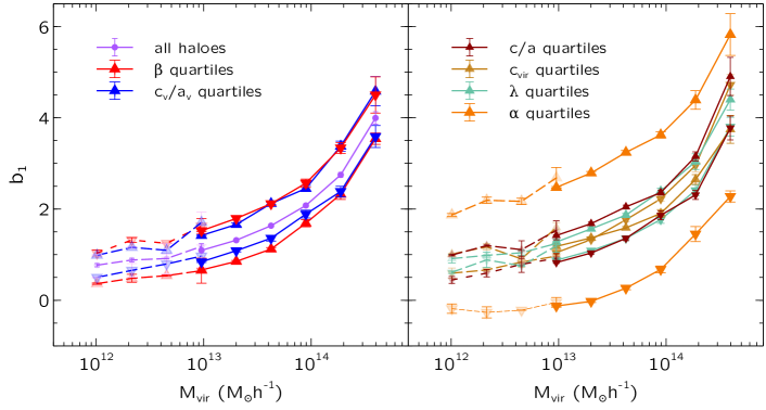
Figure 1 summarizes previously known assembly bias / secondary bias trends due to halo velocity anisotropy variables and (left panel) and halo shape , concentration , spin and tidal anisotropy (right panel). In each panel, upward (downward) triangles indicate the mean halo bias in the upper (lower) quartiles of the respective quantity, at fixed halo mass. Additionally, the circles in the left panel show the mean bias for all haloes at fixed mass.
We see that haloes that are aspherical either in shape (small ) or velocity dispersion (small ) are less clustered than more spherical haloes. The split by velocity anisotropy shows that haloes dominated by more radial orbits () are less clustered than tangentially dominated haloes. Correspondingly, haloes with smaller spin values are less clustered than those with higher spin. The split by halo concentration shows a more complex trend, with highly concentrated haloes being less clustered at high masses but more clustered at low masses, the inversion occurring near . Finally, haloes in isotropic environments (small ) are substantially less clustered than those in anisotropic environments.
The assembly bias trend with halo concentration (as well as formation time, which we don’t show here) has been widely discussed in the literature (see, e.g., Wechsler et al., 2006; Jing et al., 2007; Dalal et al., 2008; Desjacques, 2008; Angulo et al., 2008; Faltenbacher & White, 2010; Sunayama et al., 2016; Lazeyras et al., 2017; Paranjape & Padmanabhan, 2017). The inversion of the trend is related to the tidal anisotropy of the halo environment; a large fraction of low-mass haloes live in highly anisotropic and biased environments999We discuss the so-called ‘splashback’ haloes in section 4. such as cosmic filaments, unlike more isolated haloes which dominate their environment and follow the trends predicted by standard spherical collapse models (Paranjape et al., 2018a). There are also indications that the trend in velocity anisotropy may be connected to the tidal environment, with low-mass haloes accreting in filaments being dominated by tangential orbits; such haloes should inherit high values of large-scale bias from their parent filaments (Borzyszkowski et al., 2017).
The monotonic dependence of halo bias on halo asphericity and spin at fixed mass in the right panel of Figure 1 is consistent with the trends noted previously in the literature using configuration space definitions of bias (Bett et al., 2007; Gao & White, 2007; Faltenbacher & White, 2010; Johnson et al., 2018) (see also van Daalen et al., 2012, for a study of shape- and spin-dependent clustering at Mpc scales).
As regards the asphericity of the velocity ellipsoid or related variables, we are unaware of any work other than Faltenbacher & White (2010) that has discussed the corresponding assembly bias trend. It is therefore worth commenting on the nature of this trend before proceeding. We see in the left panel of Figure 1 that the amplitude of the trend with is only slightly weaker than that with . The nature of the trend is quite interesting, however, since it says that haloes with spherical velocity ellipsoids cluster less strongly than aspherical ones. On the one hand, this suggests a potential connection with the trend shown by the asphericity of the shape tensor which is qualitatively identical. On the other, it is also tempting to compare with the trend due to . Keeping in mind that perfectly spherical velocity ellipsoids would correspond to , it is clear that the trend defined by upper and lower quartiles of is actually sensitive to additional information about haloes with aspherical velocity ellipsoids, by splitting these into radially dominated (upper quartile) and tangentially dominated (lower quartile) haloes (c.f. the discussion earlier regarding the connection between and the full phase space of the halo.)
It is clear from Figure 1 that the trend between halo bias and the local tidal anisotropy is the strongest amongst all the secondary bias trends. In fact, defining at the halo radius ensures that this correlation is stronger than that between and the local overdensity of the halo environment measured at the same scale (Paranjape et al., 2018a). Moreover, the definition of is such that this variable would be statistically independent of the very large-scale overdensity in the (Gaussian random) initial conditions, unlike at the same scale (Sheth & Tormen, 2002). The fact that and correlate so strongly is then highly suggestive of a physical link between these quantities related to the non-linear dynamics of halo formation (see also Castorina et al., 2016). The strength of the correlation will be important below.

3.2 Disentangling multi-scale correlations using conditional correlation coefficients
As discussed in the Introduction, we are interested in identifying a clean statistical signature that contributions from different length scales might segregate into distinct correlations: one between internal halo properties and the local cosmic web environment and the other between the local web and large-scale halo bias. A convenient approach to addressing this issue is to use the concept of conditional correlation coefficients (Han et al., 2019), as we describe next. This analysis is made possible by our use of a halo-by-halo measurement of bias that does not require haloes to be binned.
Consider three standardized (i.e., zero mean, unit variance) Gaussian variables with mutual correlation coefficients , and . The conditional distribution is then a bivariate Gaussian with variances , and the conditional covariance
| (12) |
The key point to note is that, if , then the conditional distributions of and at fixed are independent: . Bayes’ theorem then implies that the conditional distribution of is independent of : . In the present context, to the extent that any statistical correlation between physical variables should ultimately have a physical origin, this would strongly suggest that the statistical connection between and is linked by (at least) two physical mechanisms, one connecting to and the other connecting to .
This discussion shows that the vanishing of is a useful diagnostic of the conditional independence of on . Although we phrased the discussion in terms of a multi-variate Gaussian for , the fact that this distribution is non-Gaussian is not as large a concern as one might have imagined. Rather, the significance of is tied to the assumption that can be well-approximated by a model which is linear in and (see equations 3 and 4 in Bernardi et al., 2003). It is just that, for a multi-variate Gaussian, the linear model is exact.
Nevertheless, to minimise systematic errors, we will rely on measurements of Spearman’s rank correlation coefficients for each pair of variables, which standardises all the distributions before computing correlations. Below, we will also discuss tests of the robustness of this choice of statistics.
3.3 Tidal anisotropy as an indicator of assembly bias
Our motivation behind setting up the correlation analysis in the previous section was to explore the possibility that assembly bias correlations between internal halo properties and large-scale bias might be explained using the separate correlations of each of these with some intermediate-scale environmental variable. In this context, it is worth mentioning that previous investigations of assembly bias have failed to identify any single environmental variable that might be responsible for correlations between halo bias and multiple internal halo properties (Villarreal et al., 2017; Xu & Zheng, 2018). The fact that tidal anisotropy shows by far the strongest correlation with halo bias makes a promising candidate for such a variable.
In the language of the previous section, therefore, we will now think of as the tidal anisotropy , as halo bias and as any one of the internal halo properties . Below we will also report the results of analysing other permutations and combinations of variables, including using intermediate-scale overdensity as the environmental variable.
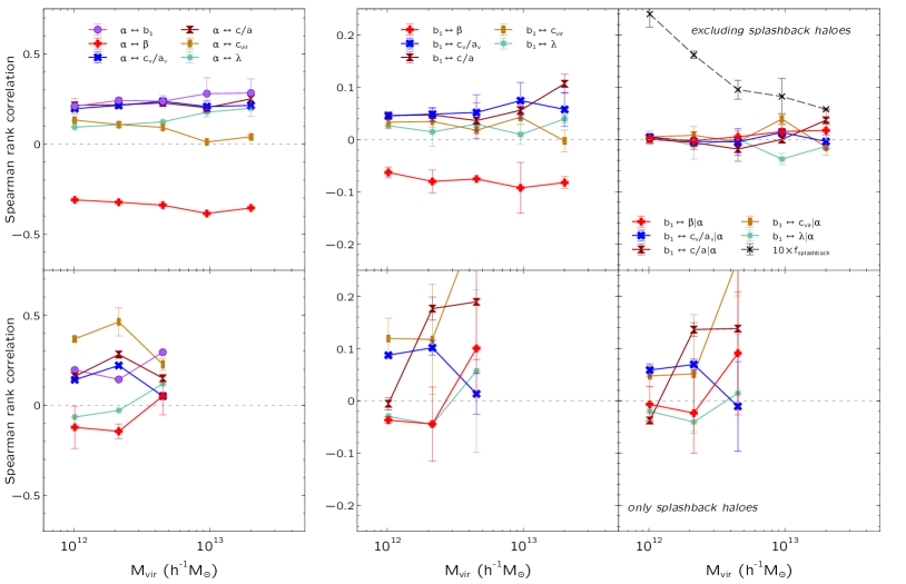
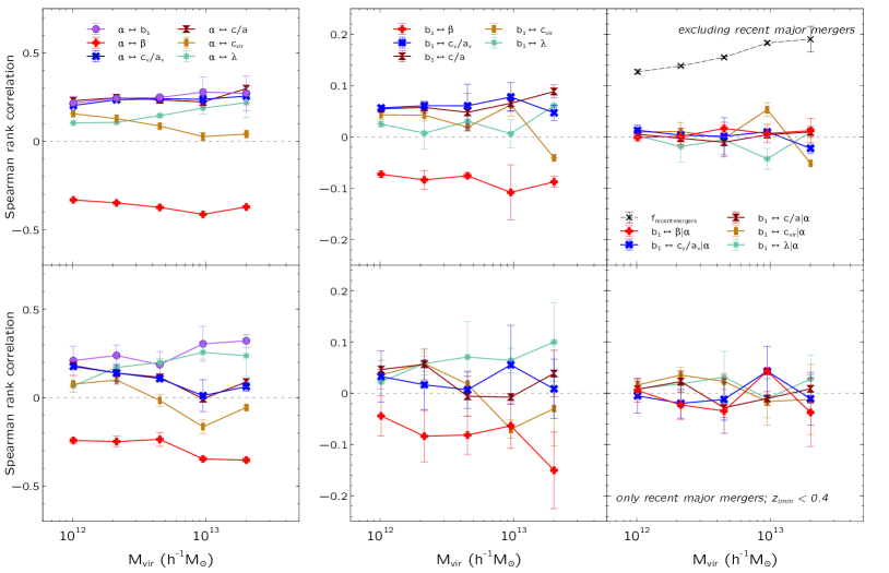
Figure 2 shows the main results of this paper. The left panel shows Spearman rank correlation coefficients (for haloes in fixed bins of )101010We have checked that all our results are robust to our choice of binning. Namely, we found identical results for all correlation trends when doubling the number of mass bins. Thus our results are unaffected by mass-dependent trends in any correlation. between the tidal anisotropy and other halo properties including halo bias and all internal properties . This panel summarizes a number of previously known results, including the observations that, at fixed mass, haloes in more anisotropic tidal environments tend to be more strongly clustered (, Hahn et al., 2009; Paranjape et al., 2018a), more concentrated (, Paranjape et al., 2018a), more spherical (, Wang et al., 2011), with higher spin (, Hahn et al., 2009; Wang et al., 2011), and have more tangentially dominated velocity distributions (, Borzyszkowski et al., 2017). Additionally, we see that objects in anisotropic environments also have more spherical velocity ellipsoids (), with a correlation very similar at all masses to that between and the mass ellipsoid asphericity .
The middle panel of Figure 2 summarizes the known assembly bias trends discussed in section 3.1. We see that the strength and sign of the correlation coeffcients at any halo mass is perfectly consistent with the results of the previous binned analysis (Figure 1) which focused on the extremes of the distributions of internal halo properties. Note that we have zoomed in on the vertical axis as compared to the left panel; the correlations of halo properties with large-scale bias are weaker (by approximately a factor in each case) than the respective correlations with the local tidal environment.
The right panel of Figure 2 shows our main new result: we display the conditional correlation coefficients (calculated using equation 12) for each internal property . The vertical scale is identical to that in the middle panel which showed the corresponding unconditional coefficients using the same scheme for colours and markers. In each case, we see that the conditional coefficients are substantially smaller in magnitude than the corresponding unconditional ones at all masses (by a factor or so at low masses). In fact, except for around (see below), the conditional coefficients are scattered around zero in all cases over the entire mass range, implying that is an excellent candidate for the primary environmental variable responsible for halo assembly bias trends. In support of this argument, we find in Appendix A.4 (see also below) that conditioning on performs much better at decreasing assembly bias strength than conditioning on at the same scale, despite the fact that and are correlated. Further, in order to quantify exactly how close to zero the conditional coefficients are in Figure 2, we use two methods.
| conditional corr. coeff. | dof |
|---|---|
| 0.90 | |
| 0.97 | |
| 1.76 | |
| 2.18 | |
| 3.13 | |
| 4.34 | |
| 11.89 | |
| 14.52 | |
| 24.00 | |
| 29.96 |
The first is a straightforward Chi-squared test which we perform using the results in 9 mass bins of the low and high resolution boxes where we have reliable error bars on the measurements of . While performing this test, we also relaxed the assumption of using as the intermediary between halo properties and bias, exploring multiple other combinations involving either the overdensity or one of the internal properties themselves as the intermediary. When the resulting triplet combinations are ordered in increasing order of reduced Chi-squared, we find that triplets involving as the intermediary produce the best Chi-squared values, while those involving perform much worse. Table 1 summarizes these results. We note that the largest discrepancy in our conclusions occurs for the assembly bias variable at high masses; the residual assembly bias conditioned on deviates from zero at masses . This can be seen in right panel of Figure 2 and also causes the largest Chi-squared values out of the five assembly bias variables in Table 1.
The second method is to simply construct the ratio : if the magnitude of this ratio is small, it means that conditioning on has indeed substantially decreased the correlation between and . This is a particularly useful diagnostic for internal properties such as halo concentration whose correlation with halo bias is the smallest in amplitude of all internal properties. The results are shown in Figure 3. For the internal properties , we see that the relative correlation coefficient is, in fact, much smaller than unity over nearly the entire halo mass range.
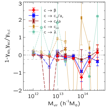
For halo concentration and spin, on the other hand, the relative correlation shows very large fluctuations and noise at higher masses. This is perhaps not surprising considering previous results which suggest that assembly bias signatures at these mass scales are likely caused by other effects (Dalal et al., 2008; Paranjape et al., 2018a). Interestingly, our results from Table 1 and Figure 3 indicate that is a particularly good indicator of spin assembly bias in the mass range -. This can be compared with the results of Johnson et al. (2018) who found that spin assembly bias can be largely explained using the presence of neighbours of comparable mass. Our results are consistent with theirs, since represents the anisotropy of the total tidal field in the halo vicinity, including the influence of all neighbours.
To summarize, the statistical correlation between large-scale bias and essentially any internal halo property that we have studied is consistent with arising from the individual correlations and , at nearly all halo masses.
3.4 Reliability of chosen statistics
We argued in section 3.2 that the use of correlation coefficients combined using equation (12) relies essentially on the implicit assumption that the underlying correlations between triplets of variables are linear. Our use of Spearman’s rank correlations means that the relevant variables are actually the ranks of the physical variables, so that we are dealing with triplets of correlated variables which are individually uniformly distributed. Although the variables are now standardized, their intrinsic correlations are not necessarily linear or even monotonic (see, e.g., Figure 12 of Paranjape et al., 2018a, which shows that the median halo concentration is non-monotonic in at fixed mass), so one might still worry about systematic effects in our analysis. We have therefore performed some explicit tests, which we describe here, to establish the robustness of our conclusions. Our method differs from that of Han et al. (2019) who used Gaussian process regression to explicitly fit for the non-linearity / non-monotonicity of the dependence of halo bias on other variables, thus allowing them to explore a multi-dimensional bias ‘manifold’. Instead, below we demonstrate the robustness of our primary results using direct probes of probability distributions involving , and one halo internal property at a time.
We first test the reliability of replacing explicit conditional correlation coefficients (which would require binning of data) with the expression in equation (12) (which uses all available data) in Appendix A.4, focusing on the strongest assembly bias signature which is that of the velocity anisotropy . Figure 11 shows that explicitly binning in before computing the correlation coefficient between and does decrease the magnitude of the correlation to nearly zero at all masses and for all .
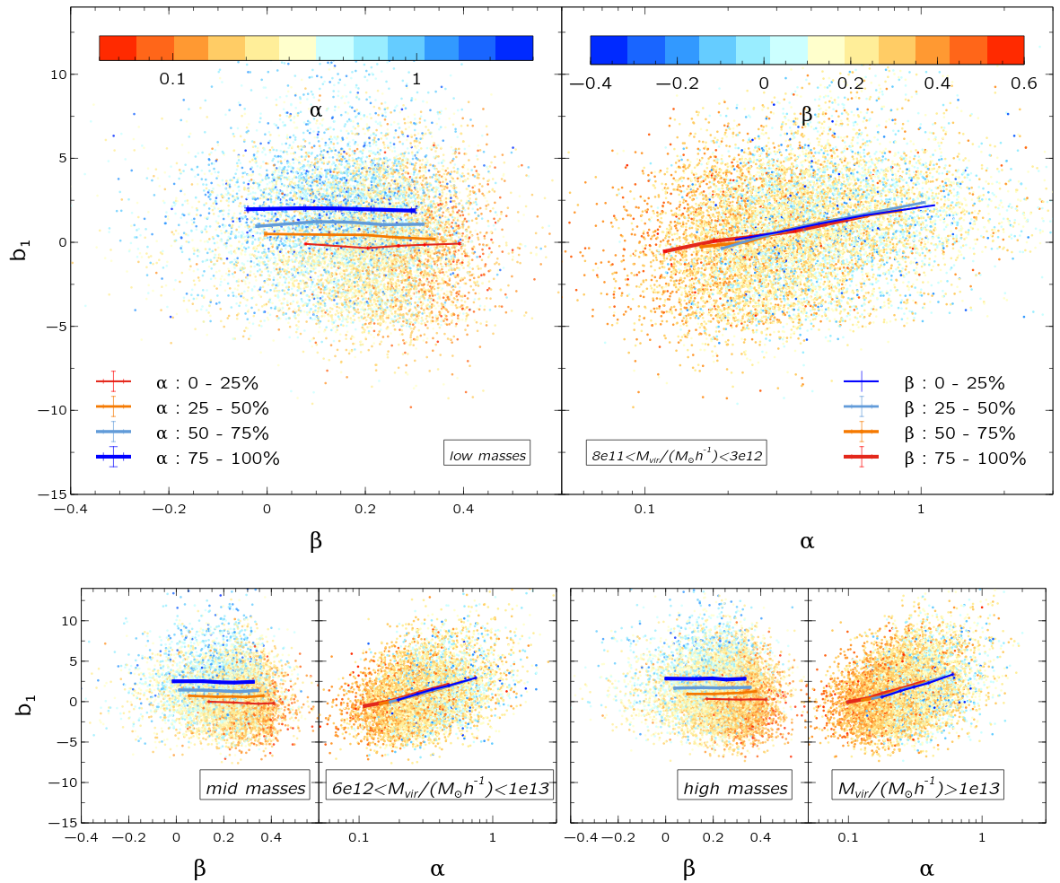
To address the concern regarding non-linearity or non-monotonicity of the intrinsic correlations, we focus on three mass ranges; low [], mid [] and high [] containing haloes each and dissect the full distribution of in Figure 4. The scatter plots in the top panels of the Figure focus on the low mass range. The top left panel shows the distribution of and , with the symbols coloured by the value of . Apart from an overall negative correlation between and (c.f. middle panel of Figure 2), we can also see that both these variables are correlated with by observing that the redder (bluer) points, which correspond to () are largely confined to the bottom right (top left) of the distribution. Similar conclusions about the correlation between variables can be made from the top right panel which shows the scatter distribution of and , with the symbols coloured by the value of .
In order to extract more information on the structure of the joint probability distribution , we consider the mean value of bias conditioned on and i.e, . In the 3-dimensional space of , this quantity forms a 2-dimensional surface whose properties we explore using projections onto the - and - planes, as we discuss next.
In the top left panel of Figure 4, we plot the projection of onto the - plane as solid lines, with each line focusing on haloes in quartiles of (from red to blue in increasing thickness as increases.) The overall assembly bias trend between and is now visible as the fact that the blue (red) curve having larger (smaller) bias lies toward smaller (larger) . More interestingly, we see that each of these lines is approximately horizontal; this implies that in each quartile of is independent of , i.e, . In other words, bias when conditioned on does not show an assemby bias with .
Similarly, the projection of onto the - plane is shown in the top right panel as solid lines, with each line focusing on haloes in quartiles of (from blue to red in increasing thickness as increases). All the lines clearly trace out the same locus of positive correlation between and , with vertical and horizontal shifts now occurring essentially in perfect tandem as changes. A simple calculation shows that this is again consistent with the relation .
These results together give a complete picture of as being approximately a plane in space and moreover being orthogonal to the - plane. The bottom panels of Figure 4 show that identical conclusions can be drawn for the mid (bottom left) and low (bottom right) mass bins. We can go even further and ask whether the conditional variance also displays the same behaviour. Figure 14 in the Appendix shows that this is indeed the case: the projections of this quantity in the - and - planes are consistent with the relation .
These results strongly suggest that the joint distribution itself (as opposed to only its first moment) has a structure consistent with and being conditionally independent of each other, when conditioned on :
which then ensures that the trends of and discussed above emerge. Thus, the overall anti-correlation between and (assembly bias) is explained by the mutual dependence of these variables on the tidal anisotropy .
We emphasize that this analysis made no assumptions regarding Gaussianity of the variables, monotonicity or linearity of the trends, etc. We have further verified that essentially identical results are obtained using all other internal halo properties considered in this work as well (see Figures 13 and 14 in the Appendix).
The results of this section therefore provide strong support for our claim that the tidal anisotropy is the primary indicator of assembly bias for a number of internal halo properties. Our tests have further demonstrated that our conclusions are robust to our choice of statistical tools (Spearman rank correlation statistics, with conditional correlation coefficients defined by equation 12). In the next section, we explore other, physical choices related to sample selection which could, in principle, affect our conclusions.
4 The impact of splashback objects and major mergers
The primary analysis of this work presented in section 3 defined haloes as objects identified as being distinct at the epoch of interest . These haloes therefore also include the small population of so-called ‘splashback’ haloes (Gill et al., 2005), which are objects that have passed through one pericenter passage of their eventual host but are currently outside its virial radius. Treating splashback objects equivalently to genuine distinct haloes therefore risks contaminating any signal that involves a correlation with large-scale environment. Indeed, there is considerable evidence that, at low masses, a significant fraction of the assembly bias signal in variables such as halo concentration or age in fact arises from splashback objects (Dalal et al., 2008; Hahn et al., 2009; Sunayama et al., 2016; Villarreal et al., 2017; Mansfield & Kravtsov, 2019). It is then important to assess the impact of this small population on our conclusions regarding the influence of the cosmic web environment.
Similarly, the fact that there are strong correlations between tidal environment and internal properties such as halo asphericity in position or velocity space could be connected to the occurrence of recent major merger events. We must therefore also ask whether the cancellations we see in the conditional correlation coefficients in the previous section are related to major mergers.
We address both of these issues in this section, showing that our results are unchanged when excluding splashback haloes or segregating haloes by the epoch of their last major merger.
4.1 Splashback objects
We identify splashback haloes using the output of consistent-trees which provides the redshift of the ‘first accretion’ event of each object. This is the epoch at which the main progenitor of the object first passed inside the virial radius of a larger object. Splashback haloes are then objects which are currently not identified as subhaloes (i.e., not inside the virial radius of a larger object; ‘PID’ according to consistent-trees) but have . With a fine time resolution in our merger tree which uses snapshots, we expect this criterion to capture most of these objects.
We have repeated the analysis of section 3 for halo samples excluding splashback haloes and also for the splashback haloes themselves. Since we only have merger histories available for haloes in our high resolution boxes, we focus on the low-mass range for this analysis. Figure 5 shows the results. We see in the top row that excluding splashback haloes has essentially no impact on our main results, since the correlation coefficients in the left and middle panels, as well as the level of cancellation in the right panel, are nearly identical to the low-mass results of Figure 2. The black curve in the top right panel shows the fraction of haloes that were excluded as being splashback objects; this is always over this mass range and decreases as expected towards higher masses.
Interestingly, when we repeat the analysis for these splashback objects themselves (bottom row of Figure 5), we see very different behaviour. Firstly, the correlation between and at the lowest masses is now weaker in magnitude than other correlations, in stark contrast to the case for distinct haloes. And the right panel shows that, in fact, has essentially no impact on the assembly bias correlations involving any internal property. (We do not display the results for the two highest mass bins which contain fewer than objects each.) In other words, the cosmic web anisotropy is a very poor indicator of any assembly bias trend for splashback objects. This is physically perhaps not surprising considering the very different accretion and tidal stripping histories of these objects as compared to other genuinely distinct haloes. We discuss this further in section 5.
4.2 Recent major mergers
The output of consistent-trees provides, for each object, the epoch of the last major merger event this object experienced on its main progenitor branch. The definition of a major merger is an event involving the overlap of virial radii of objects with a mass ratio closer to unity than . We use objects from the higher resolution box as in the earlier analysis and discard splashback objects as defined by the criterion of section 4.1. We segregate the remaining objects by their redshift of last major merger into two populations : those with recent major mergers which occurred at (corresponding to Gyr of lookback time) and those with major mergers further back in the past. We then compute the same rank correlation coefficients as before and repeat the analysis similar to that shown in Figure 5.
Figure 6 shows the results. Our segregation makes the recent major merger population have fewer objects, thus the results have larger scatter. Despite this, we see that separating out the population with recent major mergers does not bring out any dramatic difference in our main results, suggesting that both the populations of haloes are influenced similarly by their respective tidal environment as regards their assembly bias trends. We conclude that major merger events are not a likely cause for being an excellent statistical intermediary in explaining halo assembly bias.
5 Discussion & conclusion
The hierarchical formation of cosmological structure leads to distinct connections between the properties of the cosmic web and its constituent dark matter haloes across a wide range of length scales. The most striking amongst these are the ones categorized as assembly bias (or secondary bias), in which the large-scale () clustering strength of haloes shows distinct trends with a number of internal halo properties (defined at scales ), even at fixed halo mass. Understanding the origin of such correlations across several orders of magnitude in length scale is of great interest from the point of view of building a complete understanding of structure formation in the CDM framework, and can have consequences for galaxy evolution and precision cosmology.
In this work, we have explored the idea that many (if not all) assembly bias trends in the mass range could be largely a result of a multi-scale connection between internal halo properties and the large-scale environment, with the local, non-linear cosmic web environment acting as an intermediary. This is motivated by the expectation that these correlations must be connected to the only physical mechanism at play (gravitational tides) at the most natural intermediate length scale in the problem (the current turn-around radius for infalling material around a given halo, which is close to the halo radius).
We considered scalar internal properties related to the shape, velocity dispersion, density profile and angular momentum of haloes; these include the halo shape asphericity (section 2.3.1), velocity ellipsoid asphericity (section 2.3.2), velocity anisotropy (section 2.3.3), concentration (section 2.3.4) and spin (section 2.3.5). The large-scale environment of each halo was characterised using the halo-by-halo bias of Paranjape et al. (2018a) defined at scales (section 2.1) and, for the local cosmic web environment, we considered the halo-centric tidal tensor defined at scales (section 2.2), focusing on the tidal anisotropy variable (equation 4) introduced by Paranjape et al. (2018a).
Our primary statistical analysis relied on Spearman rank correlation coefficients calculated for pairs of variables. In particular, we argued that the vanishing of conditional correlation coefficients defined in equation (12) offers a useful and compact way to assess the strength of multi-variate statistical connections (section 3.2), and we further demonstrated that this technique is robust to all of the assumptions involved in using equation (12) (section 3.4 and Appendices A.4 and A.6).
Our main results can be summarised as follows.
-
•
The tidal anisotropy shows the strongest correlation by far with at fixed halo mass amongst all halo properties we have considered (Figure 1 and middle panel of Figure 2) and correlates strongly with all internal halo properties as well (left panel of Figure 2). The correlation between and in particular is substantially stronger than that between and pure density or pure anisotropy variables, as discussed in section 2.2. The variable is therefore an excellent candidate for an intermediary in explaining assembly bias, more so than the density contrast (equation 2) defined at the same scale (Appendices A.2 and A.3).
-
•
The conditional correlation coefficients are substantially smaller in magnitude than the unconditional coefficients for all internal halo properties that we studied, for all but the highest mass scales we consider (right panel of Figure 2, see also Table 1 and Figure 3). The joint distribution of , and any internal property is therefore consistent with reflecting only two fundamental correlations and :
(13) (section 3.2, see also Figure 4 and Appendix A.6). Thus, indeed explains all large-scale assembly bias trends, particularly at low halo mass. defined at the halo radius also outperforms the environmental overdensity defined at fixed smoothing scales -, recently proposed by Han et al. (2019) as an assembly bias indicator (see Appendix A.2).
-
•
Our conclusions regarding the role of are unchanged upon excluding splashback haloes from the analysis (section 4.1, top row of Figure 5). Interestingly, repeating the analysis for the small population of splashback objects themselves (these are of distinct haloes in our mass range) showed that is a poor indicator of any assembly bias trend for these objects (bottom row of Figure 5, see also below).
- •
This wide-ranging effect of in connecting small and large scales provides a new perspective on the phenomenon of assembly bias of low-mass haloes. There are several indications in the literature that multiple aspects of a halo’s tidal environment could play a role in establishing the assembly bias trends of different variables. E.g., being in a non-linear filament affects the mass accretion rate and formation time of an object (due to strong tides, Hahn et al., 2009; Musso et al., 2018) and changes its shape, profile and velocity dispersion structure (due to strong external flows, Borzyszkowski et al., 2017; Mansfield & Kravtsov, 2019). Consistently with this picture, tidal influences on substructure also start well before accretion onto the parent object (Behroozi et al., 2014). Similarly, the presence/absence of neighbours having larger (Hahn et al., 2009; Hearin et al., 2016; Salcedo et al., 2018) or comparable mass (Johnson et al., 2018), and their corresponding tidal influence, has also been shown to be connected with assembly bias. (See also Mo et al., 2005; Buehlmann & Hahn, 2019, for the related effect of tidal heating due to the formation of cosmic sheets.)
The fact that simultaneously explains multiple assembly bias trends over a wide range of halo mass suggests that, ultimately, the quantity relevant for assembly bias is the degree of anisotropy of the current tidal environment of distinct haloes, evaluated at the current turn-around scale (the halo radius). Having fixed this, the specific physical mechanism that affects any particular variable becomes less relevant; we expect it to only play a role in establishing how strongly that variable correlates with the tidal anisotropy.
This has consequences of practical interest, particularly because is defined at intermediate length scales. On the one hand, the importance of as an assembly bias indicator might be exploited to populate low-resolution simulations with otherwise unresolved haloes having the correct assembly bias trends. This would be of immense interest for precision cosmological analyses that would otherwise require high dynamic range as well as tight control on assembly bias related systematics (see, e.g., Zentner et al., 2014). On the other hand, can also be useful in high resolution, small volume simulations of galaxy formation, where it might be used to predict (albeit with large scatter) the large-scale environment of realistic galaxies. For example, understanding the strength and origin of correlations between and variables such as stellar mass, star formation rate, metallicity, etc., might help in understanding the expected strength of galaxy assembly bias, which has been difficult to detect robustly in observational samples (Lin et al., 2016; Tinker et al., 2017).
To try and understand why the variable , specifically, is such a good assembly bias indicator for distinct haloes, it is worth considering its behaviour for splashback haloes. As we showed, does not perform well in explaining the assembly bias of these objects. This is likely a manifestation of the fact that the internal properties of splashback objects, like other substructure, have been dramatically affected by the strong tidal influence of their host halo. Since this also includes substantial mass loss due to tidal stripping and a consequent decrease in radius, it is perhaps not surprising that the tidal environment evaluated at the scale the current radius, at the current location, is not a good indicator of the large-scale environment of the splashback object.
It appears, then, that is a good indicator of assembly bias for objects whose current tidal environment is the most extreme they have ever experienced, and fails for objects whose current environment does not reflect the largest tidal influences that have acted on them. This points towards a novel approach in thinking about substructure in general, in which haloes might be classified by their tidal history. Objects that have always been in tidally mild, isotropic environments (small ) would then be distinguished from objects that have spent a considerable fraction of their existence in anisotropic sheets or filaments (large ). Subhaloes and splashback objects would then simply be the extremes of the latter category, objects that have experienced very high tidal forces at some point in their past (not necessarily reflected by their current environment). Of course, for this picture to be consistent, it must also be possible to construct a local tidal indicator of large-scale assembly bias trends for subhaloes and splashback objects, perhaps defined using the scale of the host halo.
We also believe these ideas could be a useful starting point for a dynamical model of the influence of local non-linear tides on internal halo properties, building on, e.g., known results from tidal torque theory for the connection between large-scale tides and halo angular momenta and shapes (see, e.g. Catelan & Theuns, 1996) and accounting for known correlations between internal halo properties (see, e.g., Skibba & Macciò, 2011; Jeeson-Daniel et al., 2011). Finally, it would be interesting to extend our analysis to include tensor assembly bias signatures involving alignments between the mass/velocity ellipsoid tensors, angular momenta and halo-centric tidal tensors. We will return to all these issues in future work.
Acknowledgments
We thank R. Srianand, K. Subramanian, T. Padmanabhan and S. More for useful discussions, and the anonymous referee for a detailed and helpful report. The research of AP is supported by the Associateship Scheme of ICTP, Trieste and the Ramanujan Fellowship awarded by the Department of Science and Technology, Government of India. OH acknowledges funding from the European Research Council (ERC) under the European Union’s Horizon 2020 research and innovation programme (Grant Agreement No. 679145, project “COSMO-SIMS”). We gratefully acknowledge the use of high performance computing facilities at IUCAA, Pune.
References
- Alam et al. (2019) Alam S., Zu Y., Peacock J. A., Mandelbaum R., 2019, MNRAS, 483, 4501
- Allgood et al. (2006) Allgood B., Flores R. A., Primack J. R., Kravtsov A. V., Wechsler R. H., Faltenbacher A., Bullock J. S., 2006, MNRAS, 367, 1781
- Angulo et al. (2008) Angulo R. E., Baugh C. M., Lacey C. G., 2008, MNRAS, 387, 921
- Bardeen et al. (1986) Bardeen J. M., Bond J. R., Kaiser N., Szalay A. S., 1986, ApJ, 304, 15
- Behroozi et al. (2013a) Behroozi P. S., Wechsler R. H., Wu H.-Y., 2013a, ApJ, 762, 109
- Behroozi et al. (2013b) Behroozi P. S., Wechsler R. H., Wu H.-Y., Busha M. T., Klypin A. A., Primack J. R., 2013b, ApJ, 763, 18
- Behroozi et al. (2014) Behroozi P. S., Wechsler R. H., Lu Y., Hahn O., Busha M. T., Klypin A., Primack J. R., 2014, ApJ, 787, 156
- Benson (2017) Benson A. J., 2017, MNRAS, 471, 2871
- Bernardi et al. (2003) Bernardi M., et al., 2003, AJ, 125, 1866
- Bett et al. (2007) Bett P., Eke V., Frenk C. S., Jenkins A., Helly J., Navarro J., 2007, MNRAS, 376, 215
- Binney & Tremaine (1987) Binney J., Tremaine S., 1987, Galactic dynamics. Princeton University Press, Princeton, NJ
- Bond & Myers (1996) Bond J. R., Myers S. T., 1996, ApJS, 103, 1
- Bond et al. (1991) Bond J. R., Cole S., Efstathiou G., Kaiser N., 1991, ApJ, 379, 440
- Bond et al. (1996) Bond J. R., Kofman L., Pogosyan D., 1996, Nature, 380, 603
- Borzyszkowski et al. (2017) Borzyszkowski M., Porciani C., Romano-Díaz E., Garaldi E., 2017, MNRAS, 469, 594
- Bryan & Norman (1998) Bryan G. L., Norman M. L., 1998, ApJ, 495, 80
- Buehlmann & Hahn (2019) Buehlmann M., Hahn O., 2019, MNRAS, 487, 228
- Bullock et al. (2001a) Bullock J. S., Kolatt T. S., Sigad Y., Somerville R. S., Kravtsov A. V., Klypin A. A., Primack J. R., Dekel A., 2001a, MNRAS, 321, 559
- Bullock et al. (2001b) Bullock J. S., Dekel A., Kolatt T. S., Kravtsov A. V., Klypin A. A., Porciani C., Primack J. R., 2001b, ApJ, 555, 240
- Castorina & Sheth (2013) Castorina E., Sheth R. K., 2013, MNRAS, 433, 1529
- Castorina et al. (2016) Castorina E., Paranjape A., Hahn O., Sheth R. K., 2016, preprint, (arXiv:1611.03619)
- Catelan & Theuns (1996) Catelan P., Theuns T., 1996, MNRAS, 282, 436
- Dalal et al. (2008) Dalal N., White M., Bond J. R., Shirokov A., 2008, ApJ, 687, 12
- Desjacques (2008) Desjacques V., 2008, MNRAS, 388, 638
- Diemer & Kravtsov (2015) Diemer B., Kravtsov A. V., 2015, ApJ, 799, 108
- Eisenstein & Loeb (1995) Eisenstein D. J., Loeb A., 1995, ApJ, 439, 520
- Fakhouri & Ma (2010) Fakhouri O., Ma C.-P., 2010, MNRAS, 401, 2245
- Faltenbacher & White (2010) Faltenbacher A., White S. D. M., 2010, ApJ, 708, 469
- Franx et al. (1991) Franx M., Illingworth G., de Zeeuw T., 1991, ApJ, 383, 112
- Gao & White (2007) Gao L., White S. D. M., 2007, MNRAS, 377, L5
- Gao et al. (2005) Gao L., Springel V., White S. D. M., 2005, MNRAS, 363, L66
- Gill et al. (2005) Gill S. P. D., Knebe A., Gibson B. K., 2005, MNRAS, 356, 1327
- Haas et al. (2012) Haas M. R., Schaye J., Jeeson-Daniel A., 2012, MNRAS, 419, 2133
- Hahn & Abel (2011) Hahn O., Abel T., 2011, MNRAS, 415, 2101
- Hahn et al. (2009) Hahn O., Porciani C., Dekel A., Carollo C. M., 2009, MNRAS, 398, 1742
- Han et al. (2019) Han J., Li Y., Jing Y., Nishimichi T., Wang W., Jiang C., 2019, MNRAS, 482, 1900
- Hearin et al. (2016) Hearin A. P., Behroozi P. S., van den Bosch F. C., 2016, MNRAS, 461, 2135
- Heavens & Peacock (1988) Heavens A., Peacock J., 1988, MNRAS, 232, 339
- Jeeson-Daniel et al. (2011) Jeeson-Daniel A., Dalla Vecchia C., Haas M. R., Schaye J., 2011, MNRAS, 415, L69
- Jing et al. (2007) Jing Y. P., Suto Y., Mo H. J., 2007, ApJ, 657, 664
- Johnson et al. (2018) Johnson J. W., Maller A. H., Berlind A. A., Sinha M., Holley-Bockelmann J. K., 2018, preprint, (arXiv:1812.02206)
- Kaiser (1984) Kaiser N., 1984, ApJ, 284, L9
- Lacey & Cole (1993) Lacey C., Cole S., 1993, MNRAS, 262, 627
- Lazeyras et al. (2017) Lazeyras T., Musso M., Schmidt F., 2017, J. Cosmology Astropart. Phys, 3, 059
- Lewis et al. (2000) Lewis A., Challinor A., Lasenby A., 2000, ApJ, 538, 473
- Lin et al. (2016) Lin Y.-T., Mandelbaum R., Huang Y.-H., Huang H.-J., Dalal N., Diemer B., Jian H.-Y., Kravtsov A., 2016, ApJ, 819, 119
- Ludlow et al. (2010) Ludlow A. D., Navarro J. F., Springel V., Vogelsberger M., Wang J., White S. D. M., Jenkins A., Frenk C. S., 2010, MNRAS, 406, 137
- Ludlow et al. (2013) Ludlow A. D., et al., 2013, MNRAS, 432, 1103
- Ludlow et al. (2014) Ludlow A. D., Navarro J. F., Angulo R. E., Boylan-Kolchin M., Springel V., Frenk C., White S. D. M., 2014, MNRAS, 441, 378
- Mansfield & Kravtsov (2019) Mansfield P., Kravtsov A. V., 2019, preprint, (arXiv:1902.00030)
- Mao et al. (2018) Mao Y.-Y., Zentner A. R., Wechsler R. H., 2018, MNRAS, 474, 5143
- McEwen & Weinberg (2018) McEwen J. E., Weinberg D. H., 2018, MNRAS, 477, 4348
- Mo et al. (2005) Mo H. J., Yang X., van den Bosch F. C., Katz N., 2005, MNRAS, 363, 1155
- Monaco (1999) Monaco P., 1999, in Giuricin G., Mezzetti M., Salucci P., eds, Astronomical Society of the Pacific Conference Series Vol. 176, Observational Cosmology: The Development of Galaxy Systems. p. 186
- Musso & Sheth (2012) Musso M., Sheth R. K., 2012, MNRAS, 423, L102
- Musso et al. (2018) Musso M., Cadiou C., Pichon C., Codis S., Kraljic K., Dubois Y., 2018, MNRAS, 476, 4877
- Navarro et al. (1996) Navarro J. F., Frenk C. S., White S. D. M., 1996, ApJ, 462, 563
- Navarro et al. (1997) Navarro J. F., Frenk C. S., White S. D. M., 1997, ApJ, 490, 493
- Oñorbe et al. (2014) Oñorbe J., Garrison-Kimmel S., Maller A. H., Bullock J. S., Rocha M., Hahn O., 2014, MNRAS, 437, 1894
- Paranjape & Padmanabhan (2017) Paranjape A., Padmanabhan N., 2017, MNRAS, 468, 2984
- Paranjape et al. (2018a) Paranjape A., Hahn O., Sheth R. K., 2018a, MNRAS, 476, 3631
- Paranjape et al. (2018b) Paranjape A., Hahn O., Sheth R. K., 2018b, MNRAS, 476, 5442
- Peebles (1969) Peebles P. J. E., 1969, ApJ, 155, 393
- Rodríguez-Puebla et al. (2016) Rodríguez-Puebla A., Behroozi P., Primack J., Klypin A., Lee C., Hellinger D., 2016, MNRAS, 462, 893
- Salcedo et al. (2018) Salcedo A. N., Maller A. H., Berlind A. A., Sinha M., McBride C. K., Behroozi P. S., Wechsler R. H., Weinberg D. H., 2018, MNRAS, 475, 4411
- Sheth & Tormen (1999) Sheth R. K., Tormen G., 1999, MNRAS, 308, 119
- Sheth & Tormen (2002) Sheth R. K., Tormen G., 2002, MNRAS, 329, 61
- Sheth & Tormen (2004) Sheth R. K., Tormen G., 2004, MNRAS, 350, 1385
- Sheth et al. (2001) Sheth R. K., Mo H. J., Tormen G., 2001, MNRAS, 323, 1
- Shi & Sheth (2018) Shi J., Sheth R. K., 2018, MNRAS, 473, 2486
- Shi et al. (2015) Shi J., Wang H., Mo H. J., 2015, ApJ, 807, 37
- Skibba & Macciò (2011) Skibba R. A., Macciò A. V., 2011, MNRAS, 416, 2388
- Springel (2005) Springel V., 2005, MNRAS, 364, 1105
- Sunayama et al. (2016) Sunayama T., Hearin A. P., Padmanabhan N., Leauthaud A., 2016, MNRAS, 458, 1510
- Taylor & Navarro (2001) Taylor J. E., Navarro J. F., 2001, ApJ, 563, 483
- Tinker et al. (2017) Tinker J. L., Wetzel A. R., Conroy C., Mao Y.-Y., 2017, MNRAS, 472, 2504
- Villarreal et al. (2017) Villarreal A. S., et al., 2017, MNRAS, 472, 1088
- Wang et al. (2011) Wang H., Mo H. J., Jing Y. P., Yang X., Wang Y., 2011, MNRAS, 413, 1973
- Wang et al. (2018) Wang H., et al., 2018, ApJ, 852, 31
- Wechsler et al. (2002) Wechsler R. H., Bullock J. S., Primack J. R., Kravtsov A. V., Dekel A., 2002, ApJ, 568, 52
- Wechsler et al. (2006) Wechsler R. H., Zentner A. R., Bullock J. S., Kravtsov A. V., Allgood B., 2006, ApJ, 652, 71
- White & Silk (1979) White S. D. M., Silk J., 1979, ApJ, 231, 1
- Xu & Zheng (2018) Xu X., Zheng Z., 2018, MNRAS, 479, 1579
- Yan et al. (2013) Yan H., Fan Z., White S. D. M., 2013, MNRAS, 430, 3432
- Zehavi et al. (2018) Zehavi I., Contreras S., Padilla N., Smith N. J., Baugh C. M., Norberg P., 2018, ApJ, 853, 84
- Zentner (2007) Zentner A. R., 2007, International Journal of Modern Physics D, 16, 763
- Zentner et al. (2014) Zentner A. R., Hearin A. P., van den Bosch F. C., 2014, MNRAS, 443, 3044
- van Daalen et al. (2012) van Daalen M. P., Angulo R. E., White S. D. M., 2012, MNRAS, 424, 2954
Appendix A Convergence and additional tests
In this Appendix, we first present a convergence study for our calculation of tidal variables which justifies our choices for the minimum halo mass threshold in our simulations. We then show that, although the variables and defined in the main text are correlated, the tidal anisotropy is likely to be a better indicator than the isotropic overdensity of all assembly bias, an expectation which is then confirmed in the main text. We also display the 1-dimensional probability distributions of all the halo-related variables used in this work, in a few narrow mass ranges. Finally we complete our analysis in section 3.4 by showing explicitly the structure of distribution of , and for all .
A.1 Convergence study
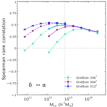
Figure 7 shows the Spearman rank correlation coefficient between and as a function of halo mass. These variables were evaluated as described in section 2.2 using various grid sizes as indicated in the legend. Results are shown for the low-resolution (markers with solid lines) and high-resolution configuration (markers with dashed lines).
We see that convergence in any given configuration of the simulations is starting to be achieved at grid sizes of cells. Based on the trends seen in Figure 7, we also choose a minimum halo mass threshold of particles as a compromise between minimising the mismatch in between the two configurations and retaining enough statistics in the highest mass bin analysed in the high-resolution simulation. A lower mass threshold would increase the mismatch, while a higher threshold such as particles would minimise the mismatch but make all measurements at the high mass end of the high-resolution box too noisy to be reliable.
Since the correlation coefficient between and is quite large across all masses, one would worry that any statements about statistical connections between and other variables such as halo bias or internal halo properties could simply be reflecting a correlation between and these properties. Below we demonstrate that this is not the case for any of the correlations we are interested in.
A.2 Tidal environment and large-scale bias
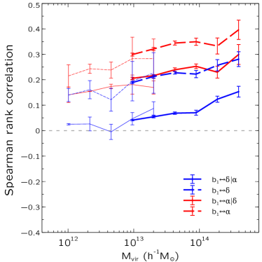
Figure 8 explores the correlations between the environment variables and defined at scales and the large-scale environment as measured by halo bias . The dashed curves show the unconditional correlation coefficients (red) and (blue). As already discussed by Paranjape et al. (2018a), these show that , so that is better correlated with than is at any halo mass. Indeed, Paranjape et al. (2018a) motivated the choice of as being the largest scale (adapted to the halo size) where this is true across all halo masses (see their Figure 5 and also the discussion below).
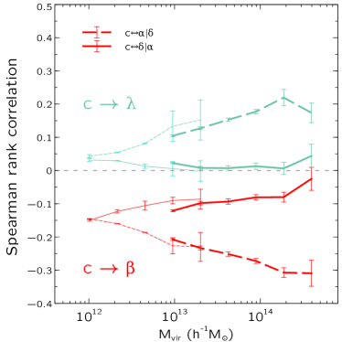
The solid curves show the conditional correlation coefficients (red) and (blue). We see that by a factor - for all halo masses. The conditional coefficient , on the other hand, shows a smaller decrement compared to the correspoding unconditional coeffcient . In fact, we curiously also see across all masses, so that conditioning on does not even decrease the correlation between and below the unconditional correlation between and .
These results indicate that is a better indicator of large-scale environment than is , both in the unconditional and conditional sense.
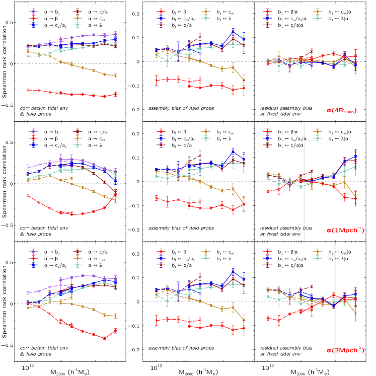
We have also repeated the analysis of Figure 2 using defined at fixed scales of and , finding that the cancellations leading to small conditional correlation coefficients only occur in the mass range where , respectively. Figure 9 shows the results. For ease of comparison, we use bins of rather than for this Figure. Finally, we have repeated this last analysis using instead of , defined at . We found that none of these variables perform as well as in producing small conditional correlation coefficients across the entire halo mass range we probe. For brevity, we do not display these results. In a recent study, Han et al. (2019) proposed that defined at - is a strong candidate for explaining assembly bias trends. Our results indicate that is an even stronger candidate, which can also be understood by the fact that the correlation seen in the left panel Figure 2 takes values at least comparable to, and usually larger than, the correlation strength between and the fixed-scale ’s (not shown).
A.3 Tidal environment and internal halo properties
Figure 10 explores the correlations between internal halo properties and the environmental variables and , colour-coded by the internal properties as in previous Figures. The solid (dashed) curves show the conditional correlation coefficients () for . We have chosen these two internal variables as representing the extremes of the trends we discuss here; the other internal variables show qualitatively identical trends with intermediate strengths. In each case, we find is substantially smaller in magnitude than at all but the smallest halo masses we explore, indicating that accounts for a substantial fraction of the correlation of with all internal properties. Especially in the case of , we see that accounts for nearly all of the correlation between and .
Taken together, the results shown in Figures 8 and 10 show that is a much better candidate than for an environmental link that could explain assembly bias in any internal halo property. In other words, the anisotropy of the halo tidal environment is expected to be more important than the local density in explaining assembly bias trends.
A.4 Explicit conditional correlation
In the main text, we explore the connection between halo tidal environment and assembly bias using the Gaussian-motivated correlation coefficients , where and represent halo bias and any internal halo property, respectively, and represents the environmental variable. Here, we perform an explicit test of this connection by evaluating correlation coefficients in fixed bins of the environmental variable. Since binning naturally increases the noise in our measurements, we only display results for the strongest assembly bias trend which is that between and velocity anisotropy .
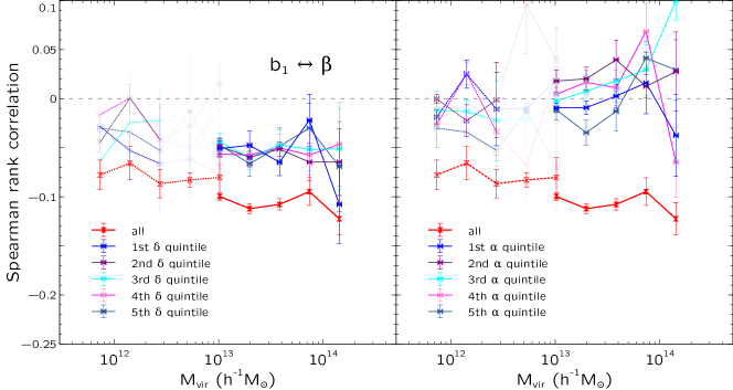
Figure 11 shows the correlation coefficients as a function of halo mass, evaluated for haloes in quintiles of (left panel) and (right panel), with the all-halo coefficient repeated in each panel in red. It is visually apparent that fixing leads to conditional correlations that are substantially closer to zero than when fixing . We have checked that qualitatively similar results hold for all other internal variables except for which the noise is too large to draw strong conclusions given our simulation set.
A.5 Halo properties
Here, we show for reference the distributions of all variables studied in the main text, including halo bias , environmental variables , and internal halo properties . See section 2 for a description of how each of these is measured.
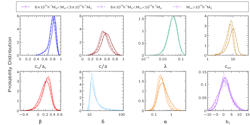
The histograms in Figure 12 show the individual distributions of all variables (different panels, as labelled) for a few narrow mass ranges (different line styles), with several known trends being apparent. We see that haloes are, on average, substantially aspherical in shape (panel ) but less so in their velocity ellipsoids (panel ), although there is a clear preference for radially dominated orbits (panel ). The distributions of spin and concentration show distinct tails at small values, while those of the environmental variables and are skewed towards large values, and the distributions of are largely symmetric around the median. All variables except and show noticeable trends with halo mass.
A.6 Joint distribution of , and internal properties
In section 3.4 we analysed the full distribution of , , and showed that the overall anti-correlation between and is consistent with being largely due to . In this section we complete this analysis by showing the same for the distribution of , and for all internal properties in all three mass ranges.
To make the results compact, we will not show scatter plots for the various distributions and instead focus on the conditional mean (as already shown in Figure 4 for the case ) and additionally the square-root of the conditional variance , for all . If the general relation (13) is true, then we should expect and . Figures 13 and 14 show that this is indeed the case, as we discuss below.
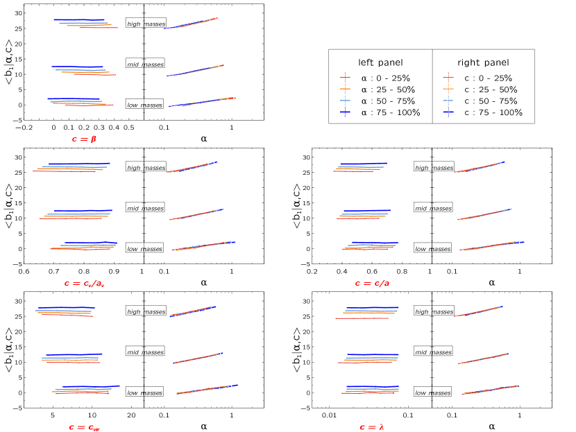
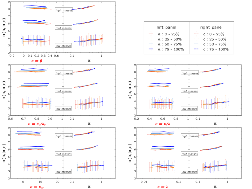
Both Figures comprise of subplots focusing on one internal variable at a time. Figure 13 (Figure 14) shows projections of () in the - (left subplot panels) and - planes (right subplot panels) for all three mass ranges (three sets of curves with offsets given for clarity). The bins along each horizontal axis are chosen as quintiles of the respective variable,111111The marker location on the horizontal axis for each such quintile is chosen as the median of that quintile, averaged over realisations. so that the left subplot panels additionally reveal the - assembly bias trends for the mean and width of the conditional distributions as systematic horizontal shifts of the different lines. Figure 13 for shows results qualitatively identical to those seen in Figure 4, with the - projections being approximately horizontal lines in fixed quartiles of , and the - projections tracing out common loci in fixed quartiles of . Figure 14 extends these results to the (square-root of) conditional variance , with the - projections again being approximately horizontal with -dependent offsets, and the - projections tracing out common loci in fixed -quartiles.
Furthermore, as we see in Figure 12, the distribution of is approximately symmetric about its mean, indicating that a Gaussian shape is a reasonable approximation. This would mean that the conditional independence of and at fixed as seen in the conditional mean and variances in fact extends to the entire distribution as discussed above. These results strongly support our main conclusions regarding the role of in explaining assembly bias.