MARTINI-based Coarse-grained Model for Poly ($\alpha$-peptoid)s

Abstract

In this paper, we present a new coarse-grained (CG) model for poly ($\alpha$-peptoid)s that is compatible with the MARTINI CG FF. In the proposed model, CG poly ($\alpha$-peptoid) is composed by a CG backbone (here we select polysarcosine as the backbone) and side chain beads. The CG model of the backbone (polysarcosine) in a solvent is first developed and then extended to poly ($\alpha$-peptoid)s with different side groups that can be obtained from MARTINI FF. We demonstrate that our CG model has good transferability. For example, the CG potentials for polysarcosine can be transferred to predict hydration free energy of other peptoids. Also, the CG polypeptoid model accurately predicts the radius of gyration over a wide range of chain lengths and the solvation free energy for relatively short peptoid molecules in good solvents. We use the CG model to study sequenced diblock polypeptoid in binary solvent mixtures and compare the results with the experimentally observed coil-globule transition.

1 Introduction

Peptoids are artificial polymers designed to mimic functions of naturally-occurring peptides. In peptides, side chains are appended to the $\alpha$-carbon, while in peptoids, side chains are attached to nitrogen atoms and form repeat units of N-substituted glycine molecules¹. The lack of both backbone chirality and backbone hydrogen bond donors in peptoids results in a variety of secondary structures. Peptoid biomimetic structure and well controllable molecular sequence² have been shown to benefit applications ranging from biomedicine to material synthesis.³ For example, peptoids have been used in biomineralization^{4, 5}, antifouling⁶, hydrate inhibitors⁷ and biorecognition sensors⁸. Similar to amino acids, peptoids can be classified as $\alpha$-peptoids, $\beta$-peptoids, and $\gamma$-peptoids according to the N-substituted group position. Among them, oligomeric $\alpha$-peptoids have been extensively investigated as peptidomimetic surrogates for medical applications. Poly($\alpha$-peptoid)s can fold into well-defined secondary structures (e.g., helices) dictated by the steric and electronic properties of the side chains. The simplest example of such structures is polysarcosine, based on the natural, non-toxic amino acid sarcosine (N-methyl glycine).⁹ In the past, polysarcosine was mostly considered in the context of synthetic polypeptides. Recently, polysarcosine have been rediscovered as a biocompatible and degradable polymer and employed in a number of drug delivery systems as micelles,¹⁰ polymersomes,¹¹ protein conjugates,¹² and nanoparticles.¹³ Furthermore, polysarcosine-based block copolymers, especially polysarcosine-co-polypeptides or co-polypeptoids, bear enormous potential to create body-compatible materials enabling the synthesis of carrier systems completely based on endogenous amino acids.¹⁴

The first polysarcosine block copolymers were reported by Gallot¹⁵ and Kimura¹⁶. Barz and co-workers further advanced synthesis methods and produced several novel functional block copolypept(o)ides.^{17, 18, 19, 20}. Despite significant progress in understanding peptoid block polymers, many challenges still remain. For example, the phase space of different side chains and conformations of polypeptoids have hardly been explored. Since laboratory experiments are difficult to perform, molecular simulations have become a popular tool for design-screening and discovery of new monomer and sequences. For example, Park and Szleifer used atomic molecular dynamics (MD) simulation to demonstrate the ability of polysarcosine and N-methoxyethyl glycine oligomers to act as anti-fouling agents when end-grafted to surfaces.²¹ Whitelam’s atomic MD simulations discovered a new secondary structure, the sigma-strand, in polypeptoid nanosheets.²² Baer’s atomic MD study of peptoid oligomers²³ improved understanding of how hydrophobic effects and ion-mediated interactions cooperate to drive assembly and folding in polypeptoids. These examples show that atomic MD methods can accurately describe the solvation behavior of peptoids in solution, including local chain orientation and intermolecular interactions at the nanometer scale. However, because of the long-range electrostatic interactions and large relaxation times of polypeptoid solutions, atomic MD simulations are too costly to simulate the intermediate structure and assembly dynamics of polypeptoids. Coarse-grained (CG) models can provide an alternative to atomistic models.²⁴ In CG models, the number of degrees of freedom in polymer repeat units is reduced in a systematic manner by representing a group of atoms or repeat units with a CG bead such that critical chemical information is retained to distinguish the interactions of various functional groups in the polymer. Therefore, a CG model can provide an in-depth picture of nanostructures and formations (e.g., a specific backbone conformation) at significantly reduced computational cost. The effective interactions between CG beads are obtained by averaging over the atomic degree of freedom. Depending on a quantity of interest, the methods to develop CG models can be classified as structure-based, force-based, and thermodynamics-based methods. The CG potentials can be obtained to reproduce microscopic (bottom-up approach) or macroscopic (top-down approach) quantities.

Two important properties of a “predictive” CG model are representability and transferability. Representability is the ability of a CG model to predict properties, other than those used to construct the CG model at the same thermodynamic “state point.” Transferability refers to the ability of a CG model developed for one kind of molecules (e.g., molecule A) at one state point to predict the same observables for the same system at different state points, or another molecule, which include the same blocks as molecule A. Here, a state point includes both physical conditions (e.g., temperature, pressure, and an external field) and chemical environment (e.g., CG bead is a fragment of a molecule). Generally, the change of state point influences the thermodynamics of solvents as well as their structure. Therefore, understanding and removing transferability-related limitations of CG models is crucial for predictive modeling of complex systems.²⁵

Several transferable CG models for polymers have been proposed. For example, a CG model of polystyrene, obtained by iterative Boltzmann inversion (IBI) method, was successfully extended to analogue poly(4-tert-butylstyrene).²⁶ However, transferability with respect to chemical conditions is more challenging to achieve. Mantha and Yethiraj²⁷ identified that the strength of the CG nonbonded interactions between water and polystyrenesulfonate changes the conformation of polystyrenesulfonate in water. This indicates that the bonded interaction between CG polymer beads could be affected by the nonbonded CG polymer–solvent interaction in a CG solvent. Sayar and co-workers investigated transferability of the diphenylalanine conformational behavior in bulk and on the interface between water and cyclohexane.²⁸ They found that a small modification of the CG model structural and conformational properties could dramatically alter its thermodynamic properties. For a polymer chain in solvent, they demonstrated that not only the torsion potential but also solvation properties of the chain fragments, as well as interactions in the environment, must be considered to reproduce the polymer conformational transition. Junghans and Mukherji²⁹ also indicated that the solvation thermodynamics is dictated by the energy density within the solvation volume of the macromolecule, the local concentration fluctuations of the solvent components, and entropic contributions. Therefore, multiple targets are needed to improve the transferability of a CG model for polymer in various solvents. Several hybrid approaches with multi-targets have been proposed to improve the transferability of CG polymer models^{30, 31}. For example, Sauter and Grafmuller³² developed a CG model of polysaccharides with combined structure-based and force-based CG approaches, which improved the transferability over both concentration and degrees of polymerization. Similarly, Abbott and Steven³³ built the CG model of poly(N-isopropyl acrylamide) (PNIPAM) by selecting density and interfacial tension as target properties that successfully captured the coil–globule transition at different temperatures. A number of CG models of proteins have been proposed in recent years ^{34, 35, 36, 37, 38}, but very few CG models of peptoids exist, and their transferability has not been demonstrated.³⁹

In this paper, we present a new CG model for poly $\alpha$-peptoids in solution that combines the structure-based and thermodynamic-based approaches (i.e., we select the local and global molecular structures and solvation free energy as targets) under the framework of MARTINI CG force field (FF).⁴⁰ We choose polysarcosine as our initial target molecule because of its simplicity and also because it serves a backbone of many poly $\alpha$-peptoids. Because of compatibility with MARTINI FF, some nonbonded interactions as interactions between beads of different solvents and sidechain beads and solvents can be directly borrowed from MARTINI FF. In our CG systems, we introduce three types of beads, including backbone, sidechain, and solvent beads. We develop CG models of polysarcosine in four solvents: water, acetonitrile, 1-octanol, and hexane. Then, the CG poly ($\alpha$-peptoid) parameters is extended to other $\alpha$-peptoids as poly (N-(2-carboxyethyl) glycine) and poly N-pentyl glycine to evaluate the transferability of the resulting CG FF. The performance of the CG poly ($\alpha$-peptoid) model in various solvents for different chain lengths is also tested. Finally, we apply the CG FF to a sequenced diblock polypeptoid in binary solvent mixtures to study the coil–globule transition and validate against experimental results.

2 Methodology and simulation details

2.1 Atomic model

In this work, the CG FF for poly ($\alpha$-peptoid) is built using a bottom-up approach. Therefore, the accuracy of atomic simulations strongly affects the CG model’s accuracy. Common protein FFs, including AMBER⁴¹ and OPLS-AA⁴², cannot accurately model peptoids.^{43, 44} In this study, we adopt Whitelam’s atomic peptoid FF,⁴⁵ which is based on CHARMM22 FF ⁴⁶ with optimized torsion interactions and charge distribution. The Whitelam peptoid FF has been validated against quantum mechanics calculations and shown to accurately represent the local structure of peptoids. We perform MD simulations of three poly ($\alpha$-peptoid)s, including polysarcosine, poly (N-(2-carboxyethyl) glycine), and poly (N-pentyl glycine). Neutral acetyl and N, N-dimethyl amide terminal groups are added to the simulated polypeptoid chains. We calculate the Gibbs solvation free energy (hereinafter referred to as solvation free energy) of polysarcosine monomer in four solvents: water, acetonitrile, 1-octanol, and hexane. The solvation free energies of poly (N-(2-carboxyethyl) glycine) and poly (N-pentyl glycine) monomer in water are also computed to test the transferability of CG parameters. To identify the effect of chain length, we calculate the solvation free energy of polysarcosine and poly (N-(2-carboxyethyl) glycine) with the length of 1, 2, 3, and 5 repeat units in acetonitrile and water. Additionally, we compute the radius of gyration ($R_{g}$) of polysarcosine and poly (N-(2-carboxyethyl) glycine) in apolar and polar solvents with the length 1, 2, 3, 5, 10, 25, 40, 50, 70, and 90 repeat units. The interaction parameters of 1-octanol, acetonitrile, and hexane are taken from the CHARMM FF, and the TIP3P model is used for water.⁴⁷ A time step of $2\text{\,}\mathrm{f}\mathrm{s}$ is used in atomic simulations. All bonds with hydrogen atoms are constrained using the LINCS algorithm.⁴⁸ The van der Waals forces are modeled as Lennard-Jones (LJ) force with a cutoff (set here to 0.9 nm for all atoms) and a force switch that smoothly interpolates the LJ function to zero at the distance between atoms equal to 1.2 nm. Long-range electrostatics is calculated using the particle-mesh Ewald summation. ⁴⁹ All modeled systems are equilibrated using isothermal-isobaric (NPT) ensemble simulations. The equilibrium time in these simulations is $20\text{\,}\mathrm{n}\mathrm{s}$ and the target temperature and pressure are 298 K and 1 atm imposed with the V-rescale thermostat and Berendsen barostat.^{50, 51} The production simulations are performed with Nose-Hoover thermostat⁵² and Parrinello-Rahman barostat.⁵³ The production simulation time is $2000\text{\,}\mathrm{n}\mathrm{s}$ in the global conformation study. The equations of motion are integrated using the velocity Verlet algorithm. We run five independent simulations for each chain length with random initial configurations in the global conformation study. Trajectories are stored every 2000 steps. All MD simulations are performed using GROMACS 5.1.2.⁵⁴ The VMD program is used to visualize the resulting molecular systems.⁵⁵

2.2 Free energy of solvation and transfer

To validate the atomic simulations and parameterize the CG FF, we calculate the solvation free energy of polysarcosine, poly (N-(2-carboxyethyl) glycine), and poly (N-pentyl glycine) in various solvents. Several methods exist to calculate the solvation free energy, including Bennett acceptance ratio method⁵⁶ (BAR), umbrella sampling method,⁵⁷ and the thermodynamic integration (TI) method.⁵⁸ Taddese and Carbone noted that the BAR method give the same result as the umbrella sampling and TI methods, while it is computationally more efficient than the TI method.⁵⁹ Therefore, in this study we employ the BAR method, as implemented in GROMACS,⁵⁴ to calculate the solvation free energy in both the atomic and CG MD simulations. The simulated systems include a single poly ($\alpha$-peptoid) monomer with acetyl and N, N-dimethyl amide terminal group solvated in a simulation box filled with: (1) 2000 water molecules, (2) 1000 1-octanol molecules, (3)  1000 hexane molecules, and (4) 1000 acetonitrile molecules. For polysarcosine and poly (N-(2-carboxyethyl) glycine), we also study the effect of chain length by modeling chain with 1, 2, 3 and 5 repeat units in acetonitrile and water. We run ten independent simulations with random initial configurations and average the solvation free energy results to eliminate the configuration dependence. All simulations are performed at $T=$298\text{\,}\mathrm{K}$$ and $P=$1\text{\,}\mathrm{a}\mathrm{t}\mathrm{m}$$. The equations of motion are integrated using the stochastic dynamics equation. The Parrinello-Rahman barostat⁵³ is used to keep pressure constant. In the calculation of solvation free energy, initial configurations in these simulations are first equilibrated by performing an energy minimization using the steepest descent algorithm, followed by a $2\text{\,}\mathrm{n}\mathrm{s}$ simulation in canonical ensemble and $5\text{\,}\mathrm{n}\mathrm{s}$ simulation in isothermal-isobaric ensemble. Then, for each solvent, $40\text{\,}\mathrm{n}\mathrm{s}$ production simulations are performed.

2.3 CG mapping and potentials

2.3.1 CG mapping

CG mapping from the atomic to coarse scale is not unique, and a mapping scheme can affect both predicting power and computation efficiency of the CG model. In our CG model of the polysarcosine (poly ($\alpha$-peptoid) backbone), we define CG beads as shown in Figure 1.

Figure 1: CG scheme (bottom) and its projection on the two-dimensional space (top) of poly ($\alpha$-peptoid) backbone (polysarcosine). The spheres (black circles in the two-dimensional projection) depict CG beads. The chemical structure of polysarcosine monomer is shown in the red circle.

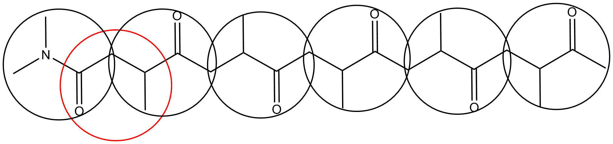
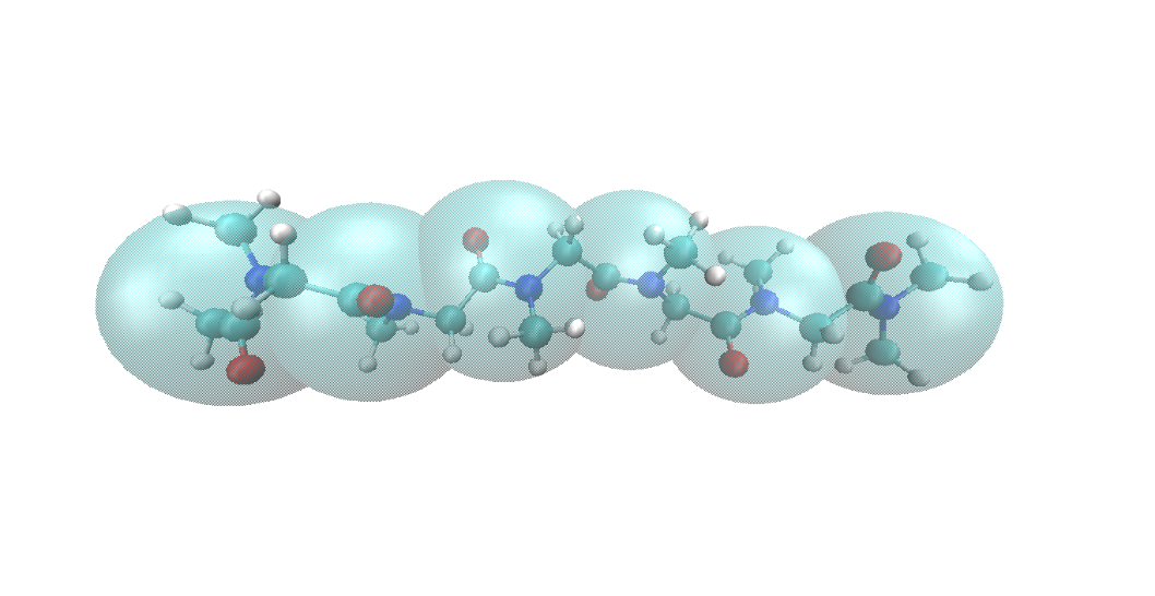
Note that each CG bead includes a half of the CH2 group and has mass of 71.076 (relative atomic mass), which is very close to that in the original MARTINI FF (each CG bead has the mass of 72). This makes the proposed CG mapping compatible with the MARTINI FF. Similar to the polybutadiene CG model,³¹ we center beads at the geometric center of the C-N bond. This choice of the bead placement allows the CG bond potential to be fitted with a simple analytical form, as described below. The solvents are modeled with CG “solvent” beads using the same degree of coarse-graining as in MARTINI FF.

Figure 2 schematically describes all types of interactions between CG beads for a typical CG poly ($\alpha$-peptoid) molecule with side chains in a solvent.

Figure 2: Interactions in the CG model of poly ($\alpha$-peptoid) molecule with side chains in solvent. The CG backbone beads are labelled as blue circles, the CG side chain beads are orange, and the solvent beads are green.

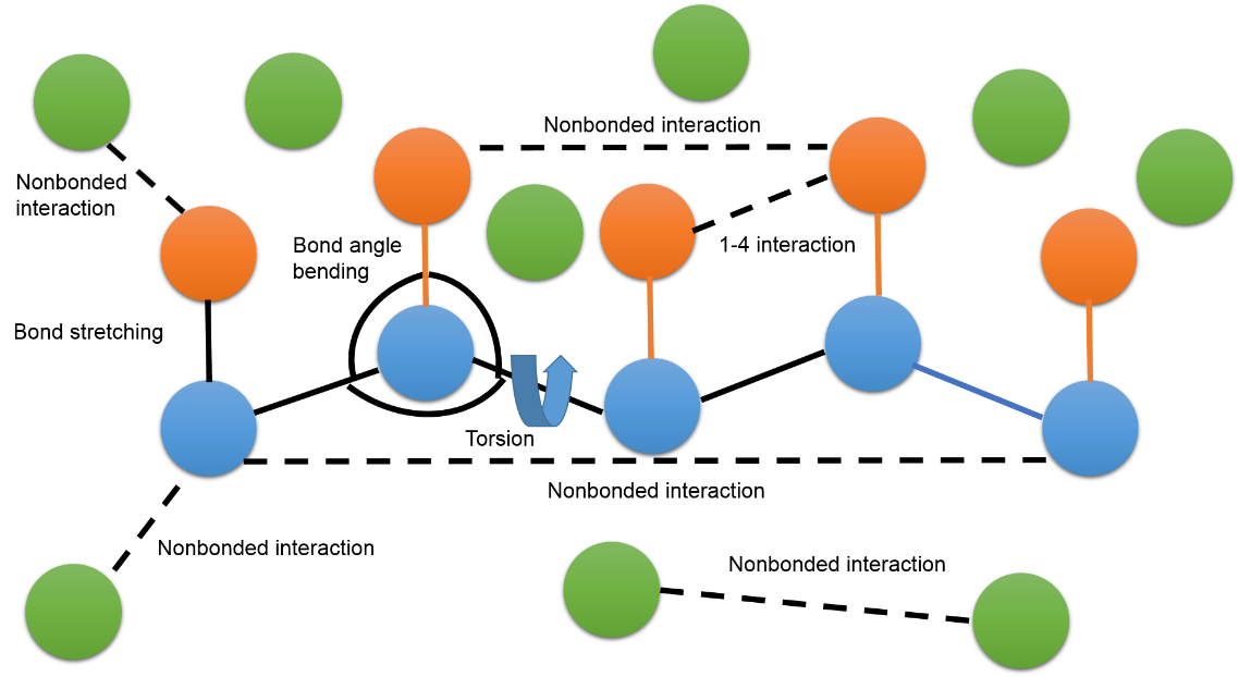
The total potential energy $U^{\text{CG}}$ due to pair and many-body interactions between CG beads, representing the backbone and side chains, consists of the bonded and nonbonded potentials:

$$U^{\text{CG}}=\sum U_{\text{bonded}}^{\text{CG}}+\sum U_{\text{nonbonded}}^{\text{CG}}.$$ (1)

In the next two sections, we discuss parameterization of these potentials.

2.3.2 Parameterization of the bonded potential in CG FF

The bonded potential, $U_{\text{bonded}}^{\text{CG}}$, can be divided into bond stretching, $U_{\text{bond}}^{\text{CG}}$, bond angle bending, $U_{\text{angle}}^{\text{CG}}$, and torsion, $U_{\text{torsion}}^{\text{CG}}$, terms:

$$U_{\text{bonded}}^{\text{CG}}\left(r,\theta,\varphi\right)=U_{\text{bond}}^{\text{CG}}\left(r\right)+U_{\text{angle}}^{\text{CG}}\left(\theta\right)+U_{\text{torsion}}^{\text{CG}}\left(\varphi\right).$$ (2)

where, $r$, $\theta$, and $\varphi$ are the bond length, bond angle, and dihedral angle, respectively. We compute $U_{\text{bond}}^{\text{CG}}(r)$, $U_{\text{angle}}^{\text{CG}}(\theta)$, and $U_{\text{torsion}}^{\text{CG}}\left(\varphi\right)$ from atomic simulations using the Boltzmann inversion method⁶⁰ as:

$$U_{\text{bond}}^{\text{CG}}\left(r\right)=-k_{B}T\text{ln}\left(\frac{P_{\text{bond}}^{\text{CG}}\left(r\right)}{r^{2}}\right)+C_{r},$$ (3)

$$U_{\text{angle}}^{\text{CG}}\left(\theta\right)=-k_{B}T\text{ln}\left(\frac{P_{\text{angle}}^{\text{CG}}\left(\theta\right)}{\text{sin$\theta$}}\right)+C_{\theta},$$ (4)

$$U_{\text{torsion}}^{\text{CG}}\left(\varphi\right)=-k_{B}T\text{ln}\left(P_{\text{torsion}}^{\text{CG}}\left(\varphi\right)\right)+C_{\varphi}.$$ (5)

Here, $P_{\text{bond}}^{\text{CG}}\left(r\right)$, $P_{\text{angle}}^{\text{CG}}\left(\theta\right),$ and $P_{\text{torsion}}^{\text{CG}}\left(\varphi\right)$ are the probability density functions (PDFs) of the bond lengths, bond angles, and dihedral angles between CG beads. The positions of CG beads are found from the atomic MD simulation of a given peptoid in a desired solvent. We apply the Boltzmann inversion method to compute CG bonded potentials for polysarcosine and poly (N-(2-carboxyethyl) glycine) in acetonitrile. The CG model of poly (N-pentyl glycine) is parameterized by transferring bonded potential for interaction between backbone beads from the polysarcosine CG model and using MARTINI FF for the bonded potential between backbone and sidechain beads. The transferability of bonded potentials $P_{\text{bond}}^{\text{CG}}\left(r\right)$, $P_{\text{angle}}^{\text{CG}}\left(\theta\right),$ and $P_{\text{torsion}}^{\text{CG}}\left(\varphi\right)$ between backbone beads is based on the assumption that these potentials are the same for the considered peptoids in any good solvent.

In Figure 3a, we see that $P_{\text{bond}}^{\text{CG}}\left(r\right)$ between backbone beads of polysarcosine in acetonitrile has Gaussian distribution. Therefore, the bond potential between the backbone beads can be accurately represented with the harmonic function:

$$U_{\text{bond}}^{\text{CG}}\left(r\right)=\frac{1}{2}k_{r}(r-r_{0})^{2}.$$ (6)

Figure 3: PDFs of (a) bond length, (b) bond angle, and (c) dihedral angle of the CG polysarcosine in acetonitrile obtained from atomic simulations.

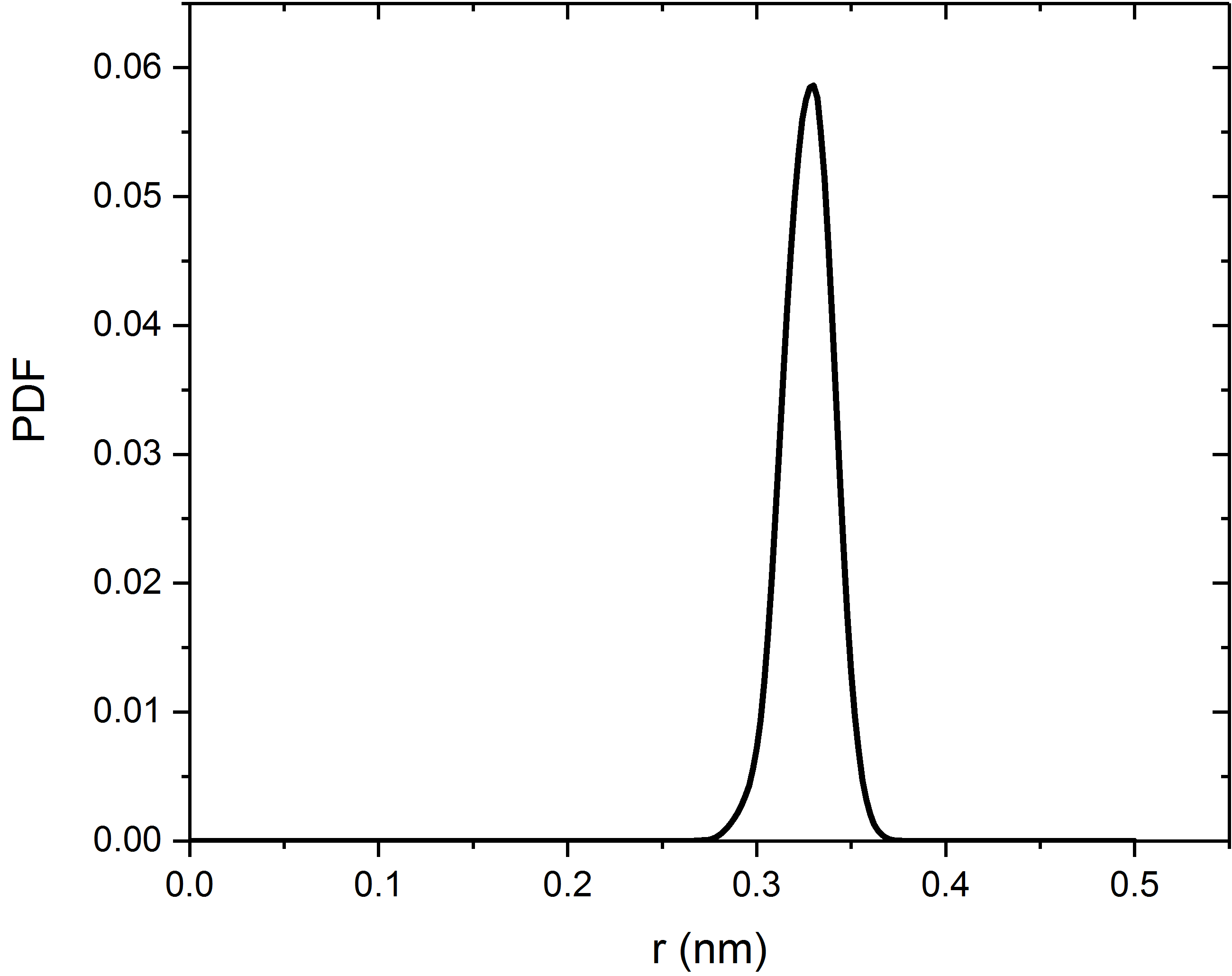
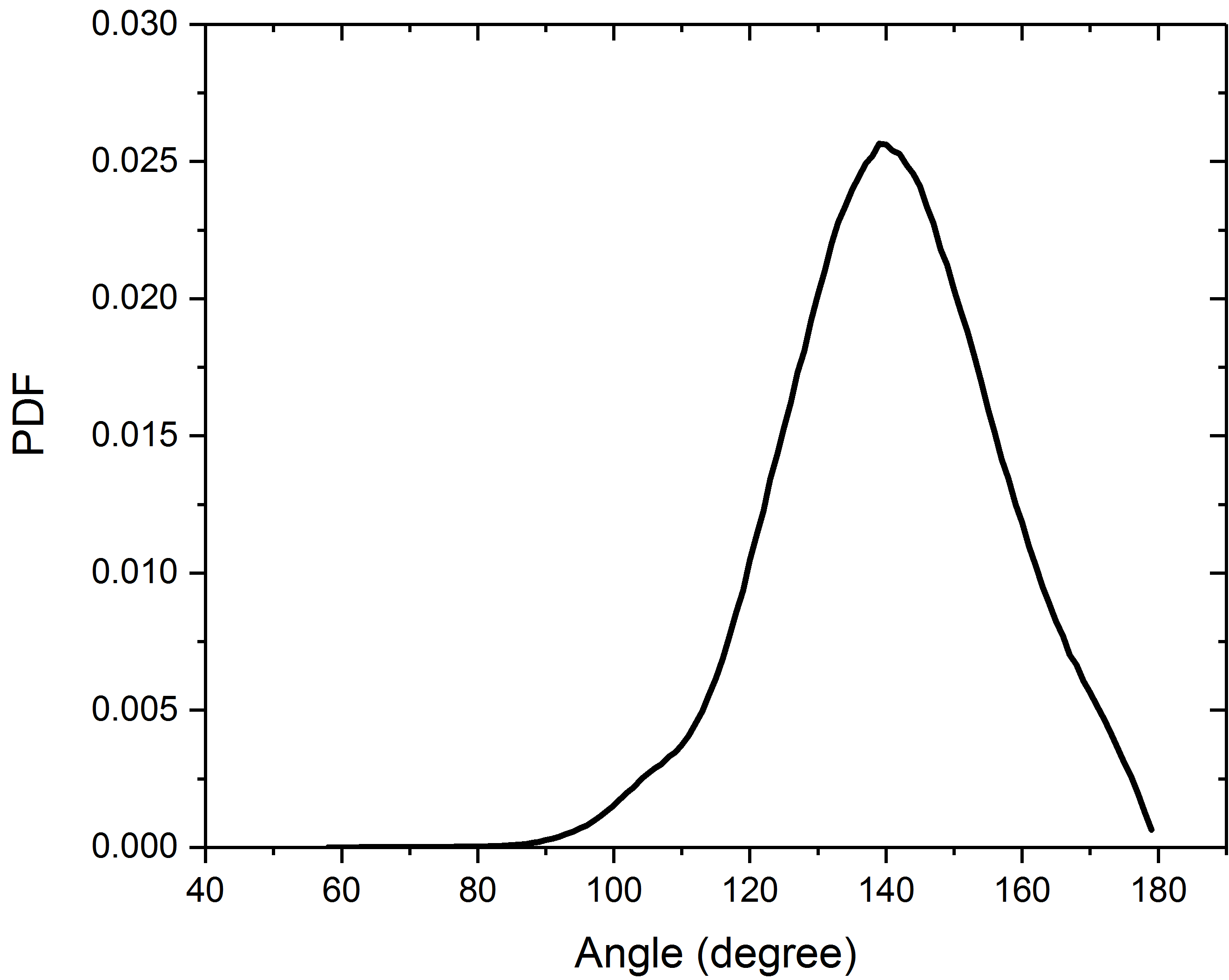
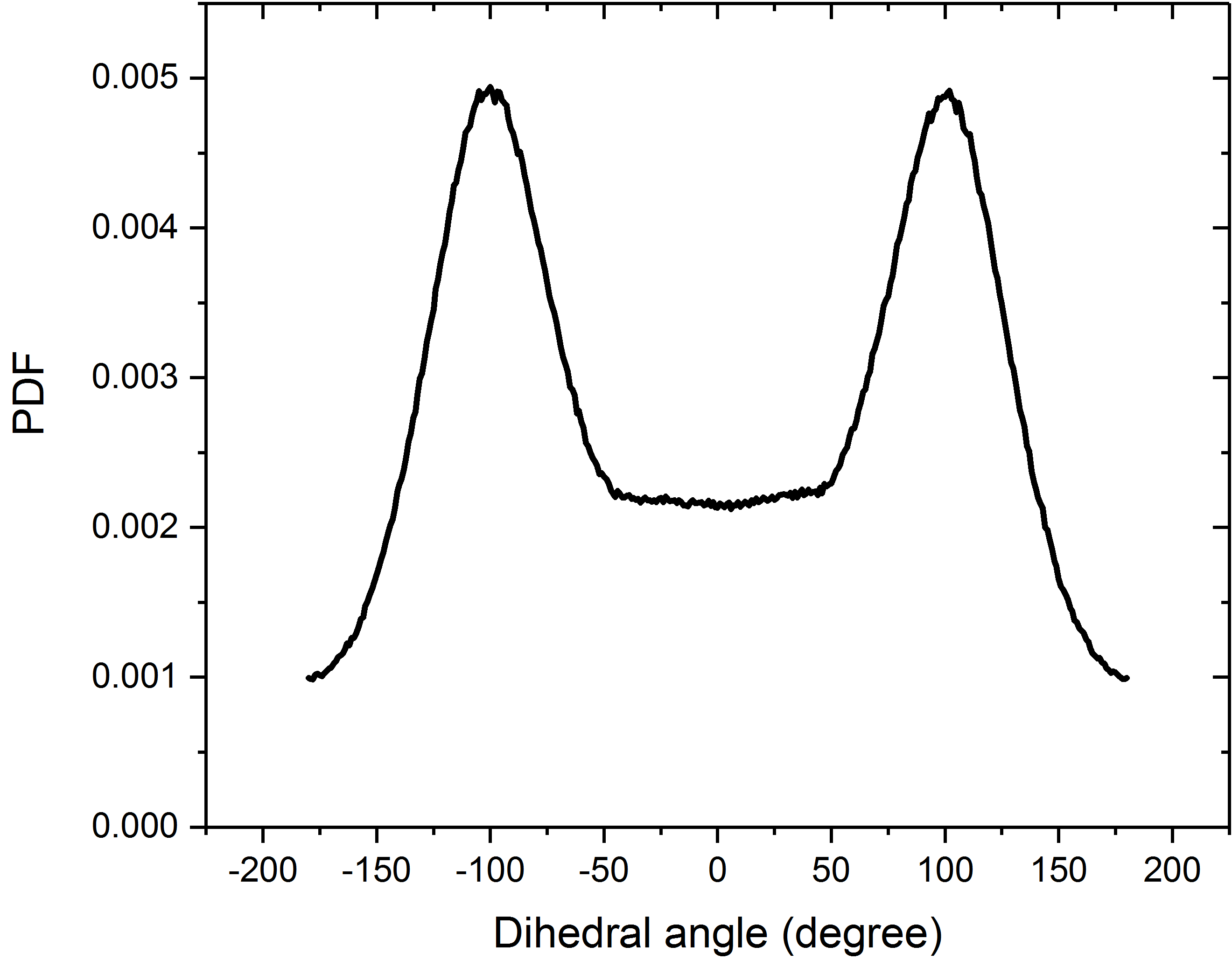
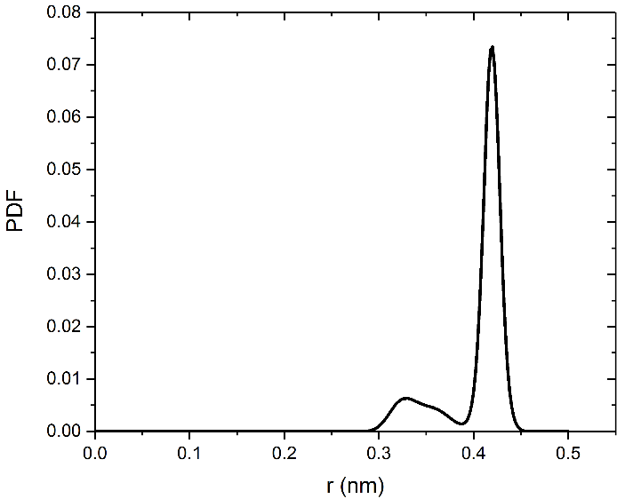
Figure 4 demonstrates that for poly (N-(2-carboxyethyl) glycine) chain in acetonitrile, $P_{\text{bond}}^{\text{CG}}\left(r\right)$ between backbone and side chain has a bimodal distribution. Therefore, $U_{\text{bond}}^{\text{CG}}\left(r\right)$ for this peptoid does not have a simple representation, and we prescribe it in a tabulated form. We also find that PDFs $P_{\text{angle}}^{\text{CG}}\left(\theta\right),$ in polysarcosine (Figure 3b) and other petoids (for bonds between two backbone and backbone and side-chain beads) have non-Gaussian distributions. Therefore, the bond angle potentials $U_{\text{angle}}^{\text{CG}}$ are given in the tabulated form.

Figure 4: The bond PDF between backbone and sidechain CG beads for poly (N-(2-carboxyethyl) glycine) in acetonitrile obtained by analyzing the trajectory in atomic simulations.

We find that the torsion potential between the backbone beads has a symmetric bimodal distribution and, therefore, can be well approximated with the analytical function ⁶¹

$$U_{\text{torsion}}^{\text{CG}}\left(\varphi\right)=\sum_{n=0}^{5}(-1)^{n}k_{n}(cos\varphi)^{n}.$$ (7)

All CG bonded interactions are listed in Tables LABEL:Tab:stretching–3. Similar to Huang’s CG poly(methyl methacrylate) model⁶², we disregard the torsion potentials between backbone and side-chain beads and two neighbor side-chain beads. To avoid the overlap between beads due to the disregarded torsion potential, the “1-4” nonbonded interactions between backbone and side-chain beads and two side-chain beads (see Figure 2) are included in the form of the LJ 12-6 potential

$$U_{\text{nonbonded}}^{\text{CG}}=4\varepsilon\left[\left(\frac{\sigma}{r}\right)^{12}-\left(\frac{\sigma}{r}\right)^{6}\right].$$ (8)

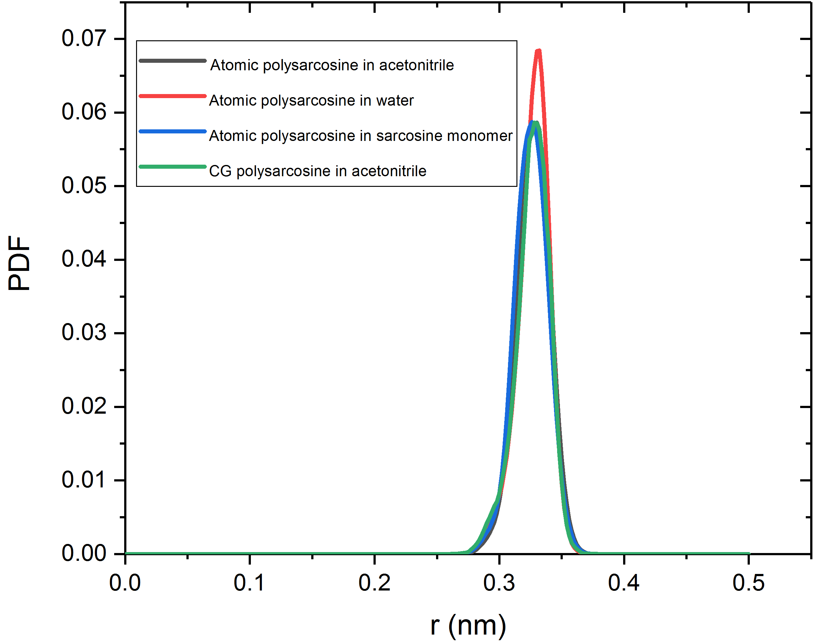
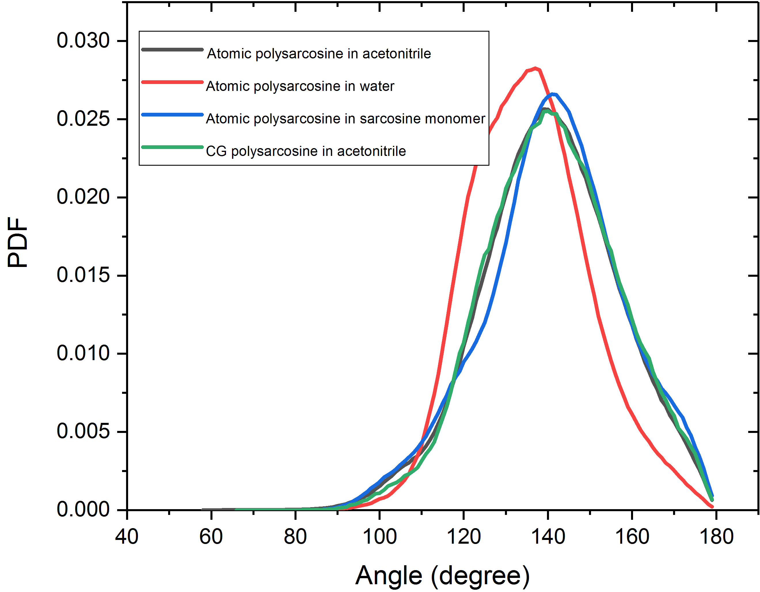
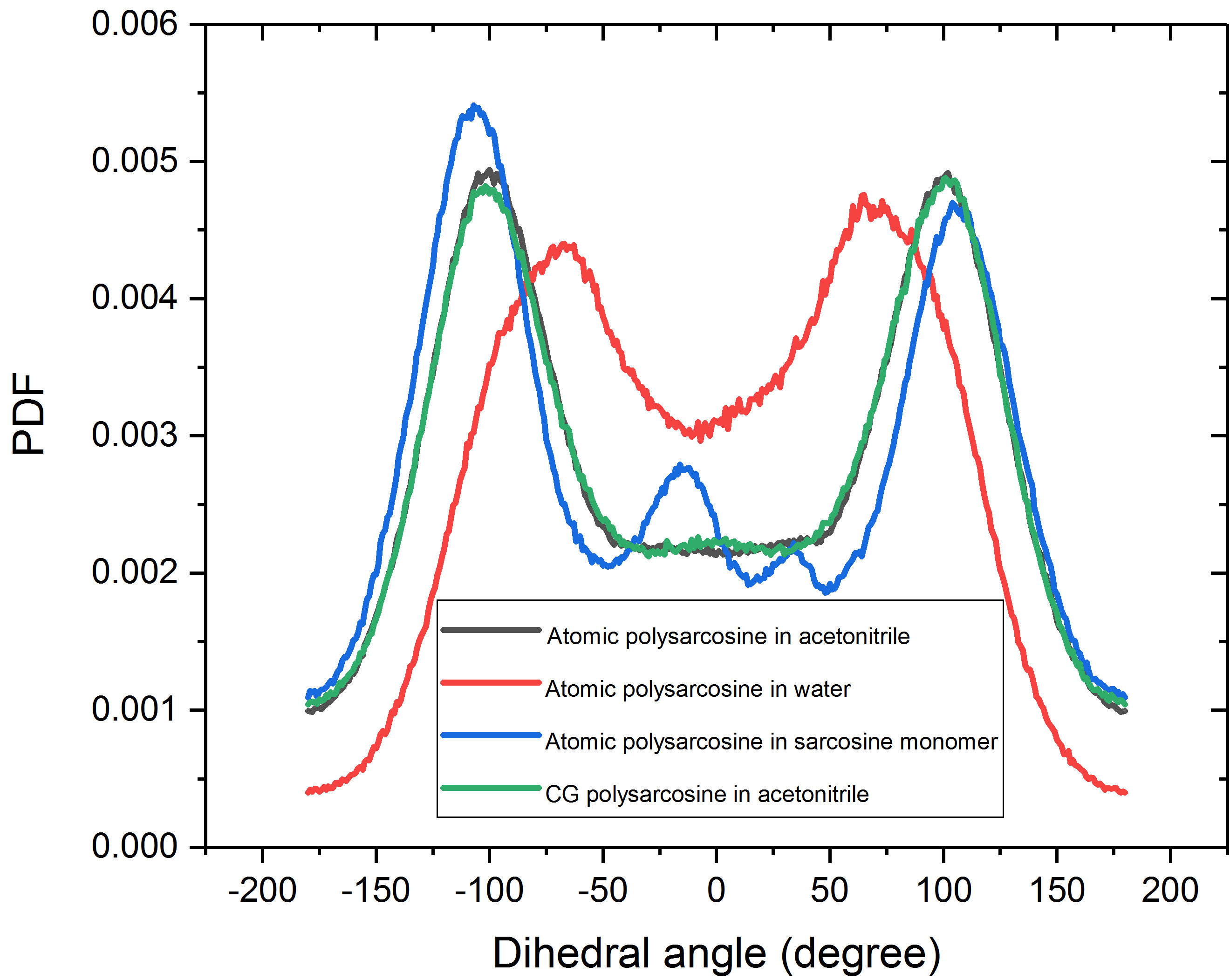
To evaluate the dependence of local structures on solvent types, we analyzed the atomic simulation trajectory of polysarcosine chain in a CG manner (i.e., we determine locations of CG beads from atomic simulations as described in Figure 1 and obtain the PDFs for the bond length, bond angle, and dihedral angle of CG polysarcosine chain in acetonitrile, water and sarcosine monomer. Figure 5, shows that the proposed CG model can reproduce the local conformation of polysarcosine in acetonitrile. This figure also demonstrates that PDFs of bond length and angle are practically independent of the solvent type. On the other hand, the PDF of dihedral angle show strong dependence on the solvent type. This implies that the CG bond and angle potentials are transferable in various solvent, but the torsion potential may not be transferable.

Figure 5: (a) PDF of bond, (b)PDF of angle, (c)PDF of dihedral angle of CG polysarcosine in CG acetonitrile, water and sarcosine monomer obtained from atomic simulations.

Table 1: CG Bond stretching potential for the polysarcosine between sarcosine (backbone) CG beads (denoted as PA) and acetic group (side chain) beads (denoted as P3). This naming convention follows the MARTINI FF.

Bond stretching	$k_{\text{r}}$(KJ/mol)	$r_{\text{0}}$(nm)
PA-PA	17000	0.332
PA-P3	Tabulated (see Figure S1)

Table 2: CG Bond angle bending potential for polysarcosine.

Bond angle bending	k(KJ/mol)	$\theta$(degree)
PA-PA-PA	Tabulated (see Figure S1)
PA-PA-P3	Tabulated (see Figure S1)

Table 3: CG torsion potential for polysarcosine.

Torsion	$k_{0}$(KJ/mol)	$k_{1}$(KJ/mol)	$k_{2}$(KJ/mol)	$k_{3}$(KJ/mol)	$k_{4}$(KJ/mol)	$k_{5}$(KJ/mol)
PA-PA-PA-PA	0.19054	$-1.59509$	3.61401	3.56366	$-0.76257$	$-0.62289$

2.4 Parametrization of the nonbonded potentials in the CG FF

Following the MARTINI FF, for the nonbonded interaction potential we use the LJ 12-6 potential (8). In the LJ 12-6 potential, the parameter $\sigma$ represents the closest distance between two CG beads and $\varepsilon$ is the strength of their interaction. The nonbonded interactions act between beads of a peptoid chain and solvent, between beads of different chains, and also between beads on the same chain separated by three beads or more.

In the original MARTINI FF, the magnitude of $\sigma$ depends on the degree of coarse graining and is set to $\sigma=$ $0.47\text{\,}\mathrm{n}\mathrm{m}$ for the 4:1 CG mapping (four heavy atoms mapped to one “large” CG bead) and $\sigma=$ $0.43\text{\,}\mathrm{n}\mathrm{m}$ for the 3:1 CG mapping (“small” beads). The $\varepsilon$ value depends on the types of CG beads. The interactions between CG beads are divided into four main types: polar (P), nonpolar (N), apolar (C), and charged (Q). Each main type has five subtypes, which are distinguished by the hydrogen-bonding capabilities or the degree of polarity. The range of $\varepsilon$ is from 2.0 to $5.6\text{\,}\mathrm{K}\mathrm{J}\mathrm{/}\mathrm{m}\mathrm{o}\mathrm{l}$.⁴⁰ For convenience, it is divided in 10 levels in the MARTINI FF. Each level is “fine-tuned” to reproduce the experimentally observed solubilities. In this work, we consider four solvents: water, hexane, 1-octanol, and acetonitrile. Depending on types of interacting beads, we compute $\sigma$ and $\varepsilon$ by matching Rg or solvation free energy. For some solvents, $\sigma$ and $\varepsilon$ can be found in the original MARTINI FF. All nonbonded interaction pairs in this study, as well as the methods used for estimating the $\sigma$ and $\varepsilon$ parameters for each pair, are listed in Table 4.

Table 4: CG nonbonded interaction pairs in the poly ($\alpha$-peptoid) solution. Sarcosine=PA, water=P4, Acetonitrile=Snd1, n-butyl group=P1, n-butanol group=C1, Hexane=SC1, Acetic group=P3. R=obtained by matching $R_{g}$, S=obtained by matching solvation free energy, M=original MARTINI FF. TBD=not discussed in this work. For 1-octonal CG model, it is a combination of CG n-butyl group and CG n-butanol group.

Pair	PA	P4	SNd1	C1	P1	SC1	P3
PA	R	S	S	S	S	S	S
P4		M	S	M	M	M	M
SNd1			S	TBD	TBD	TBD	S
C1				M	M	M	M
P1					M	M	M
SC1						M	M
P3							M

2.5 Parametrization of the nonbonded potentials of CG acetonitrile bead

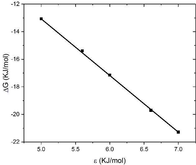
As shown in Table 4, for all considered solvents, except acetonitrile, $\sigma$ and $\varepsilon$ are given in the original MARTINI CG FF and its extensions. Note that MARTINI CG FF uses the P4 type bead for water, SC1 for hexane, and P1+C1 for 1-octanol. Because of the acetonitrile chemical properties, the type of acetonitrile beads should be one of N or P subtypes. We find that none of these subtype beads can reproduce the solvation free energy computed from atomic simulation. Therefore, we define a new CG bead subtype SNd1 for CG acetonitrile bead with $\sigma_{SNd1-SNd1}=$0.43\text{\,}\mathrm{n}\mathrm{m}$$ (according to the MARTINI rule for interactions between beads made of three heavy atoms). The parameter $\varepsilon_{SNd1-SNd1}$ for the potential between acetonitrile beads is obtained by computing solvation free energy as a function of $\varepsilon$. Figure 6 presents the relationship between $\varepsilon$ and the corresponding solvation free energy for CG acetonitrile solvated in acetonitrile solvent. The solvation free energy linearly decreases with increasing $\varepsilon_{SNd1-SNd1}$. We obtain $\varepsilon_{SNd1-SNd1}=$6.570\text{\,}\mathrm{K}\mathrm{J}\mathrm{/}\mathrm{m}\mathrm{o}\mathrm{l}$$ to reproduce the solvation free energy $\mathrm{\Delta}G=-19.51\pm$0.04\text{\,}\mathrm{K}\mathrm{J}\mathrm{/}\mathrm{m}\mathrm{o}\mathrm{l}$$ calculated from the atomic simulation. Note that this value exceeds the range of 2–$5.6\text{\,}\mathrm{K}\mathrm{J}\mathrm{/}\mathrm{m}\mathrm{o}\mathrm{l}$ for $\varepsilon$ in the original MARTINI FF.

Next, we parameterize the LJ potential for interaction between SNd1 (acetonitrile) and P4 (water) beads. The $\sigma_{SNd1-P4}$ value for this potential is set to $0.47\text{\,}\mathrm{n}\mathrm{m}$. The interaction parameter $\varepsilon_{SNd1-P4}=$4.520\text{\,}\mathrm{K}\mathrm{J}\mathrm{/}\mathrm{m}\mathrm{o}\mathrm{l}$$ is found as above to match the solvation free energy of water in acetonitrile, $\Delta G=-13.75\pm$0.12\text{\,}\mathrm{K}\mathrm{J}\mathrm{/}\mathrm{m}\mathrm{o}\mathrm{l}$$, found from the atomic simulation. Also, our atomic simulation results are in good agreement with the experimental values $\mathrm{\Delta}G=-20.29\pm 0.84$ KJ/mol for acetonitrile self-solvation free energy and $\mathrm{\Delta}G=-16.23\pm 2.51$ KJ/mol for water in acetonitrile ⁶³.

Figure 6: The self-solvation free energy of CG acetonitrile versus interaction parameter $\varepsilon_{SNd1-SNd1}$.

2.6 Parametrization of the nonbonded potentials between CG polysarcosine and solvent beads.

We determine the CG potentials between considered peptoids and any solvent in this section. Specifically, we compute the CG nonbonded potentials between polysarcosine monomer and water, 1-octanol, acetonitrile or hexane. In the original MARTINI CG FF, the glycine residue, which is similar to sarcosine, is labelled as type P5⁶⁴. Using the MARTINI FF for interaction between P5 bead and water, we obtain the hydration free energy $-40\text{\,}\mathrm{k}\mathrm{J}\mathrm{/}\mathrm{m}\mathrm{o}\mathrm{l}$, which is significantly larger than the hydration free energy of polysarcosine monomer ($-48.16\text{\,}\mathrm{k}\mathrm{J}\mathrm{/}\mathrm{m}\mathrm{o}\mathrm{l}$) computed from the atomic simulation. Therefore, we define a new bead type, PA, for the CG polysarcosine monomer bead and compute the nonbonded interaction parameters between PA and solvent beads to reproduce the hydration free energy of polysarcosine monomer (see Figure 7 for chemical structure details) in the atomic simulation.

Figure 7: The atomic and CG chemical structure of polysarcosine, Poly (N-(2-carboxyethyl) glycine), and Poly (N-pentyl glycine) monomers with terminal groups.

Figure 8: The hydration free energy of CG polysarcosine monomer versus $\varepsilon$

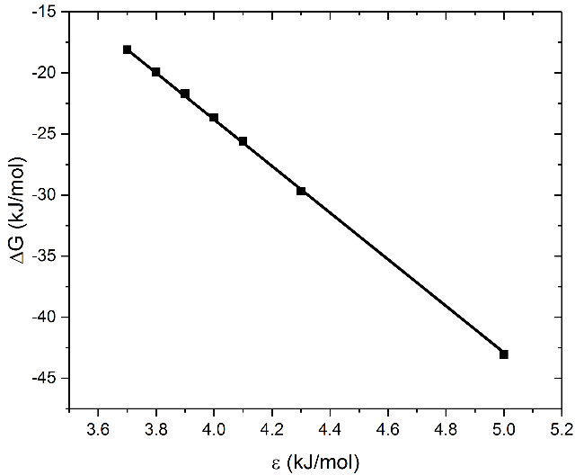
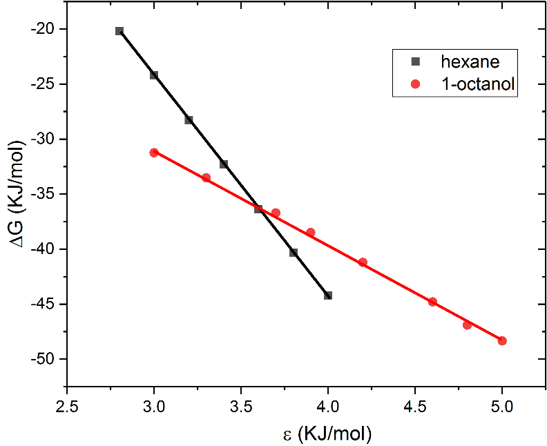
Figure 8 shows that the hydration free energy linearly decreases as $\varepsilon$ increases. We find $\varepsilon_{PA-P4}$ = $5.264\text{\,}\mathrm{k}\mathrm{J}\mathrm{/}\mathrm{m}\mathrm{o}\mathrm{l}$ that reproduces the desired hydration free energy by linear fitting. This $\varepsilon$ value is smaller than the interaction ($$5.6\text{\,}\mathrm{k}\mathrm{J}\mathrm{/}\mathrm{m}\mathrm{o}\mathrm{l}$)$ between glycine and water beads in the MARTINI CG FF. Also, it is consistent with the fact that the polarity of a sarcosine molecule is smaller than the polarity of a glycine molecule. We also use the same method to obtain $\varepsilon$ in the potentials acting between polysarcosine and other solvents CG beads, including 1-octanol, acetonitrile and hexane. Figure 9 shows the solvation free energy of polysarcosine monomer in hexane as a function of $\varepsilon$. From this figure, we find $\varepsilon_{PA-SC1}=$3.197\text{\,}\mathrm{K}\mathrm{J}\mathrm{/}\mathrm{m}\mathrm{o}\mathrm{l}$$. For 1-octanol, the estimation of $\varepsilon$ is complicated because in MARTINI FF, 1-octanol molecules comprise of two CG beads with different types (P1 and C1). We first determine $\varepsilon_{PA-C1}$ in the potential acting between PA and C1 beads. Next, we find $\varepsilon_{PA-P1}=$4.851\text{\,}\mathrm{k}\mathrm{J}\mathrm{/}\mathrm{m}\mathrm{o}\mathrm{l}$$ by matching solvation free energy in the corresponding atomic simulation (The red one in Figure 9). The solvation free energy of polysarcosine monomer in four solvents obtained in CG and atomic simulations are listed in Table 5.

Figure 9: The solvation free energy of polysarcosine monomer in 1-octanol and hexane vs interaction parameter $\varepsilon$.

Table 5: Solvation free energy of polysarcosine monomer in various solvents computed from atomic and CG simulations.

$\Delta$G(KJ/mol)	$\Delta$$G_{\text{acetonitrile}}$	$\Delta$$G_{\text{hydration}}$	$\Delta$$G_{\text{1-octanol}}$	$\Delta$$G_{\text{hexane}}$
atomic	$-49.41\pm 0.20$	$-48.16\pm 0.06$	$-47.32\pm 0.47$	$-28.21\pm 0.08$
CG	$-49.31\pm 0.24$	$-48.39\pm 0.10$	$-47.33\pm 0.17$	$-28.27\pm 0.14$

2.7 Parametrization of the nonbonded potentials between CG peptoid beads.

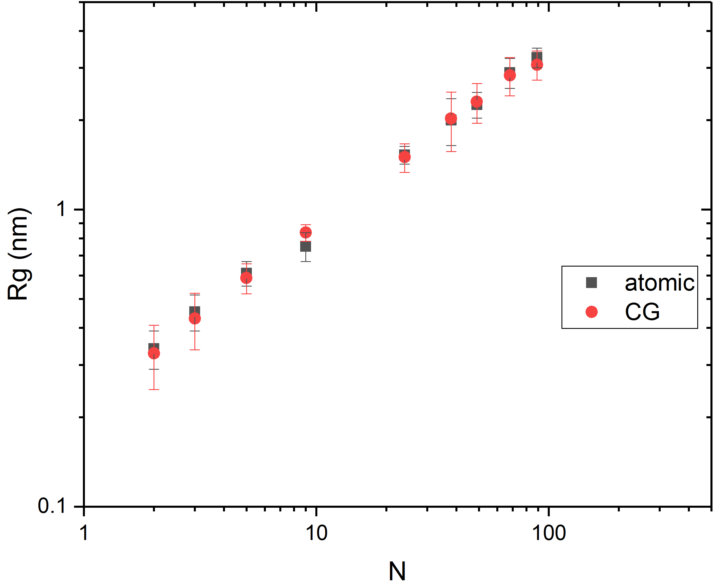
In the above section, we show how to parameterize the nonbonded potential between poly ($\alpha$-peptoid) backbone (polysarcosine) and solvent beads. Since the intramolecular nonbonded interactions are excluded for polysarcosine chain with length less than four repeat units, the interaction parameter between CG sarcosine repeat units does not affect the solvation free energy of polysarcosine monomer. Here, we compute $\varepsilon_{PA-PA}$ for polysarcosine CG beads by matching the $R_{g}$ for polysarcosine chain with 25 repeat units in acetonitrile obtained from the atomic simulations. We select acetonitrile in the calculation of $R_{g}$ because it was experimentally found to be a good solvent for polysarcosine.⁶⁵ Our atomic simulations show that $R_{g}$ has a power law behavior as a function of the number of repeat units (see Figure 10) with the scaling exponent 0.575, which, according to Flory’s theory, ⁶⁶ also confirms that acetonitrile is a good solvent for polysarcosine. Then, we obtain $\varepsilon_{PA-PA}$ = $5.6\text{\,}\mathrm{K}\mathrm{J}\mathrm{/}\mathrm{m}\mathrm{o}\mathrm{l}$ to match the $R_{g}$ of polysarcosine with 25 repeat units. The comparison of $R_{g}$ as a function of the repeat unit number, obtained from CG and atomic simulations, is shown in Figure 10. The good agreement demonstrates transferability of the nonbonded potential, i.e., $\varepsilon_{PA-PA}$ obtained from a simulation of a chain with 25 repeat units accurately predicts $R_{g}$ of chains with other number of repeat units.

Figure 10: $R_{g}$ of polysarcosine in acetonitrile with repeat units number N in atomic and CG simulations.

Theoretically, the solvation free energy of a polypeptoid with side chain in the CG model depends on the nonbonded potential between CG polypeptoid backbone and side chain. For example, the solvation free energy of Poly (N-(2-carboxyethyl) glycine) is a function of $\varepsilon_{PA-P3}$. Therefore, the interaction parameter $\varepsilon$ could be determined by matching the free energy in an atomic simulation of peptoid with two repeat units (as was done to determine parameters in Figures 8 and 9). However, we performed CG simulations of poly (N-(2-carboxyethyl) glycine) with two repeat units with several $\varepsilon_{PA-P3}$ values and found no obvious difference in the resulting solvation free energy (see Table S1). Therefore, we set it to $\varepsilon_{PA-P3}=$4\text{\,}\mathrm{K}\mathrm{J}\mathrm{/}\mathrm{m}\mathrm{o}\mathrm{l}$$, which corresponds to the level III value in MARTINI FF. This parameter can be further optimized with long poly ($\alpha$-peptoid) chain if needed. Parameters of all CG nonbonded potentials are listed in Table S2.

To further test transferability of the CG FF, we calculate the hydration free energy for the polysarcosine, poly (N-(2-carboxyethyl) glycine) and poly N-pentyl glycine and $R_{g}$ for polysarcosine and poly (N-(2-carboxyethyl) glycine) in acetonitrile. The production simulation time is $1000\text{\,}\mathrm{n}\mathrm{s}$ for calculating $R_{g}$ and $50\text{\,}\mathrm{n}\mathrm{s}$ for estimating the hydration free energy. Additionally, we simulate a CG sequenced diblock peptoid chain with 100 beads in a binary mixture of water and acetonitrile for $1000\text{\,}\mathrm{n}\mathrm{s}$ and calculate its $R_{g}$. In these simulations, the repeat unit for the diblock polymer includes four sarcosine and one (N-(2-carboxyethyl) glycine) CG beads and the acetonitrile concentration varies from 0 to $200\text{\,}\mathrm{m}\mathrm{o}\mathrm{l}\mathrm{/}\mathrm{L}$. In CG production simulations, constant temperature and pressure are maintained using Nose-Hoover thermostat⁵² and Parrinello-Rahman barostat.⁵³ The LJ potential has the cutoff distance of $1.2\text{\,}\mathrm{n}\mathrm{m}$ with smoothing after $0.9\text{\,}\mathrm{n}\mathrm{m}$.⁵⁴ Electrostatic interactions are not included in the CG model. The time step in CG simulations is $10\text{\,}\mathrm{f}\mathrm{s}$. All the CG simulations are performed by GROMACS  5.1.2. The results of these simulations are discussed in the following section.

3 CG model transferability and simulations of peptoid folding

3.1 Transferability of the CG backbone parameters to other polypeptoids with respect to hydration free energy

Here, we study the transferability of the CG parameter obtained for polysarcosine to other polypeptoids. We select poly (N-(2-carboxyethyl) glycine) and poly (N-pentyl glycine) as typical examples of peptoids with hydrophilic or hydrophobic side chains and simulate them with atomic and CG models. The chemical structures of these peptoids are shown in Figure 7. Note that in the CG models, the nonbonded interaction parameters for the new side chains are directly taken from the MARTINI FF. Table 6 presents the calculated hydration free energies of poly (N-(2-carboxyethyl) glycine) and poly (N-pentyl glycine) monomer in both atomic and CG simulations. The difference of less than 5% indicates good transferability of the CG backbone parameters obtained to other peptoids and compatibility of the proposed CG peptoid model with the MARTINI FF.

Table 6: Hydration free energy of poly (N-(2-carboxyethyl) glycine) monomer and poly (N-pentyl glycine) monomer in atomic and CG simulations

$\Delta$$G_{\text{hyd}}$(KJ/mol)	Poly (N-(2-carboxyethyl) glycine)	Poly (N-pentyl glycine)
atomic	$-64.04\pm 0.09$	$-35.45\pm 0.22$
CG	$-66.30\pm 0.17$	$-38.85\pm 0.18$

3.2 Transferability with respect to $R_{g}$

According to the Flory theory, $R_{g}$ $\propto N^{v}$ in polymer solutions, where $N$ is the number of repeat units and $\nu$ is the Flory parameter.⁶⁶ The parameter $\nu$ is 0.59 for a good solvent and 0.30 for a poor solvent. Figure 10 shows results of atomic and CG simulations of polysarcosine in acetonitrile. We see that $R_{g}$ in both the atomic and CG simulations increases with $N$. The $R_{g}$ obtained in CG simulations are in good agreement with the atomic results. The fitted $\nu$ from CG simulations is 0.591, which is consistent with the Flory theory.⁶⁶

Figure 11: $R_{g}$ of poly (N-(2-carboxyethyl) glycine) in acetonitrile as a function of the repeat units number $N$ in CG simulation.

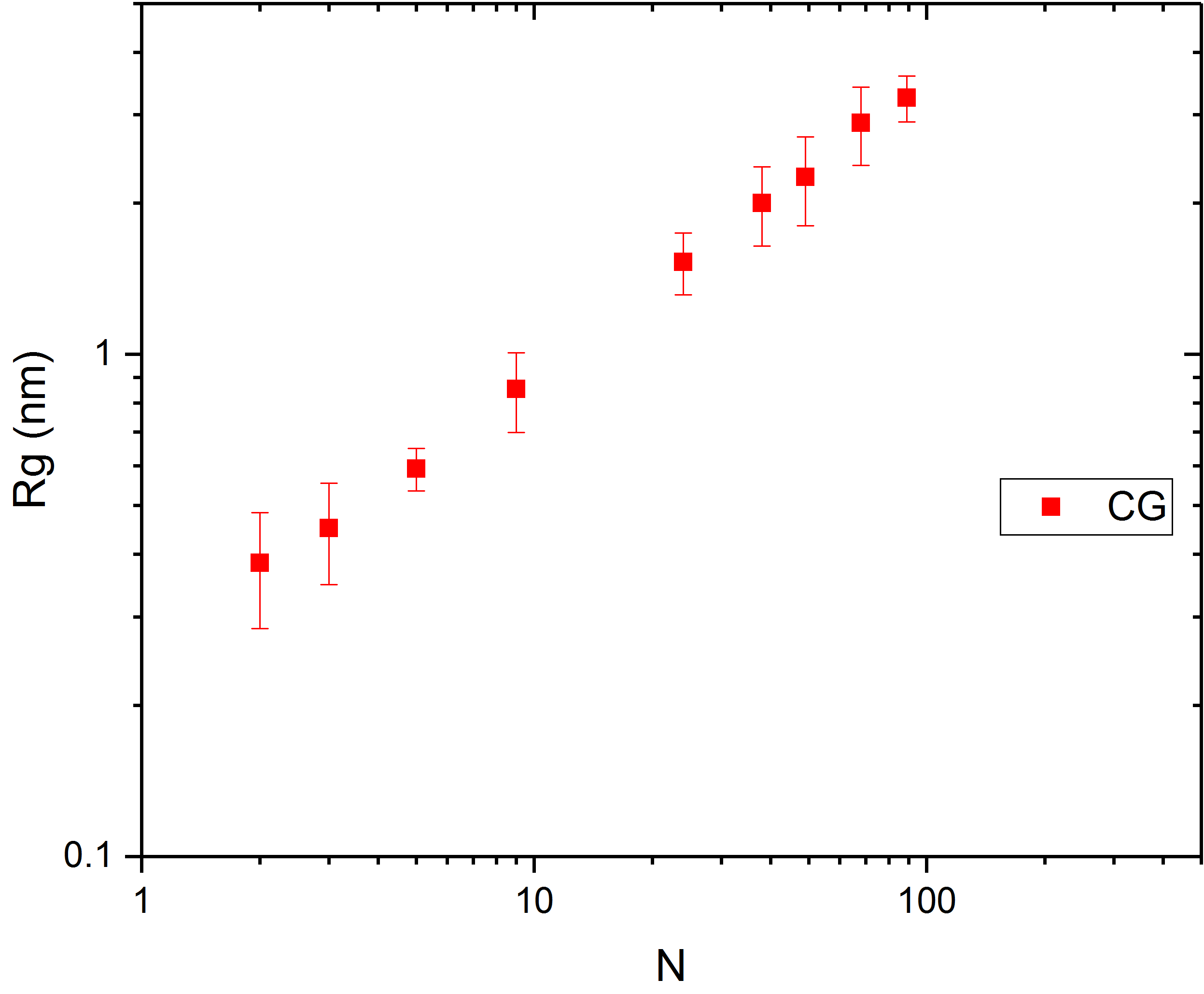
Figure 11 presents $R_{g}$ as a function of $N$ of poly (N-(2-carboxyethyl) glycine) in acetonitrile obtained with CG model. The fitted slope $\nu$ is 0.583, which is close to the theoretical value $\nu=0.59$ for a peptoid in a good solvent. Note that $\varepsilon_{P3-SNd1}$= $4.497\text{\,}\mathrm{K}\mathrm{J}\mathrm{/}\mathrm{m}\mathrm{o}\mathrm{l}$ is smaller than $\varepsilon_{P3-P3}$= $5.0\text{\,}\mathrm{K}\mathrm{J}\mathrm{/}\mathrm{m}\mathrm{o}\mathrm{l}$ in the MARTINI FF, where P3 denotes side-chain bead of poly (N-(2-carboxyethyl) glycine) and SNd1 stands for acetonitrile bead. This parameterization would lead to the peptoid chain collapse as a result of strong attraction between side chains, which makes acetonitrile behave as a poor solvent. Therefore, in the proposed CG model, we reduce $\varepsilon_{P3-P3}$ to $4.0\text{\,}\mathrm{K}\mathrm{J}\mathrm{/}\mathrm{m}\mathrm{o}\mathrm{l}$. Note that in practice, poly (N-(2-carboxyethyl) glycine) side chains deprotonate and get solvated by acetonitrile⁶⁷, keeping only a portion of hydroxyl groups. Because of this, a very few hydrogen bonds are formed between poly (N-(2-carboxyethyl) glycine) side chains. The deprotonation cannot be accurately represented in classical MD simulation that assumes a permanent chemical bond between hydrogen and oxygen atoms in the hydroxyl group. As a result, in classical MD simulation it would predict more hydrogen bonds between side chains so that the chain collapses. Therefore, we do not use the atomic results as the reference for this system.

Figures 10 and 11 demonstrate that in the proposed CG model, the bonded and nonbonded potentials estimated for polysarcosine can be transferred to the CG model of poly (N-(2-carboxyethyl) glycine) in good solvents. The transferability of bond stretching and bond angle bending potentials to similar molecules was also observed in other CG models.³⁰ Here, we show that the torsion potential also can be transferred in a properly constructed CG model. Note that not all CG potentials of polymer model are transferable. For example, in the study of CG polyethylene oxide (PEO) model,⁵⁹ nonbonded and bonded interactions derived under different CG FFs could not be combined to accurately predict the behavior of PEO chain in water.

3.3 The effect of chain length on solvation free energy

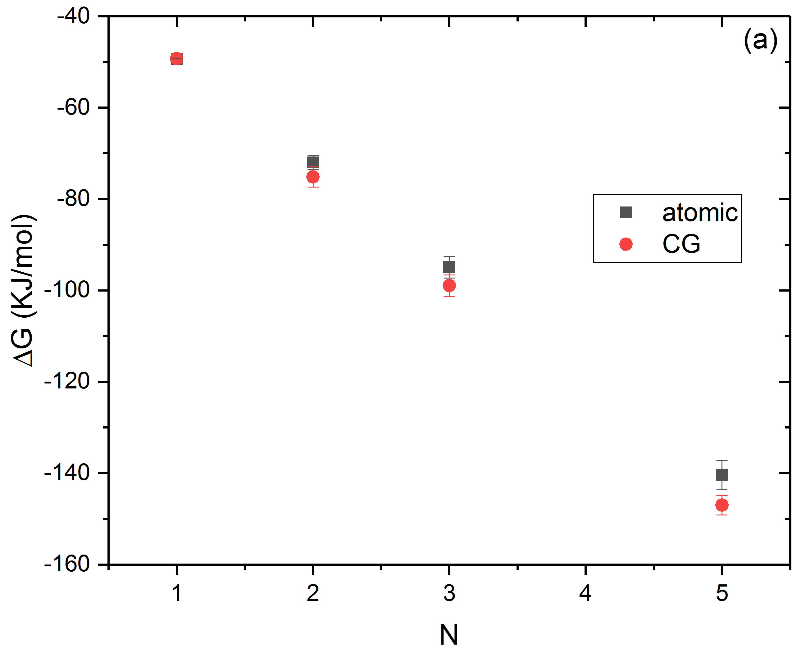
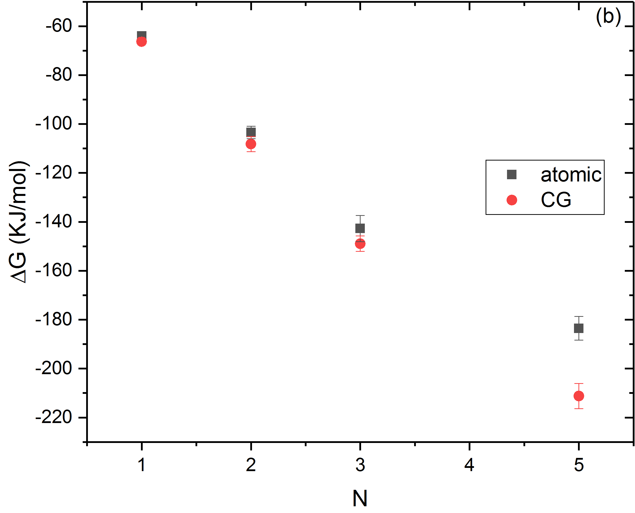
We investigate the effect of chain length on the solvation free energy of polysarcosine and poly (N-(2-carboxyethyl) glycine). Figure 12 reports the solvation free energy of polysarcosine in acetonitrile and poly (N-(2-carboxyethyl) glycine) in water as a function of the repeat unit number $N$, obtained from CG and atomic simulations. We can see that in both atomic and CG simulations, the solvation free energy increases with $N$ for both peptoids. Furthermore, we see that the CG model is transferable with respect to free energy, i.e., it can reproduce the solvation free energy of polysarcosine in acetonitrile and poly (N-(2-carboxyethyl) glycine) in water within 6% (except for the poly (N-(2-carboxyethyl) glycine) in water with $N=5$ where the error is about 16%). A possible reason for the weaker transferability of the CG model for poly (N-(2-carboxyethyl) glycine) in water is that it does not take into account the effect of the hydrogen bonding between the hydroxyl groups. In the atomic model of poly (N-(2-carboxyethyl) glycine) in water, the hydrogen bonding can be formed between the hydroxyl groups on the side chain, which affects the conformation of the backbone. Our atomic simulations show that as the chain length increases, the poly (N-(2-carboxyethyl) glycine) chain tends to collapse in water. Since the CG torsion potential is obtained from a polysarcosine in a good solvent (acetonitrile), it predicts a more extended conformation of poly (N-(2-carboxyethyl) glycine) in water. Because of the high computational cost of the BAR estimate of $\Delta G$, we limit our study the maximum chain length $N=5$ in atomic simulations.

Figure 12: (a) Solvation free energy of polysarcosine in acetonitrile with increasing number of repeat units. (b) Solvation free energy of poly (N-(2-carboxyethyl) glycine) in water with increasing number of repeat units.

3.4 Coil-to-globule transition of polypeptoid chain

Polymer collapse is the simplest form of protein folding, which is caused by the intramolecular interactions and solvent entropy. In this section, we use our CG model to study unfolding of an initially coiled polysarcosine/poly (N-(2-carboxyethyl) glycine) diblock polypeptoid chain in water-acetonitrile mixture. The choice of this peptoid is motivated by the experiments⁶⁵ on the coil-to-globule transition, where the hydrophobic interactions are concluded to be the major driving force of the peptoid chain collapse.

Figure 13: The scheme of coil-to-globule transition for diblock peptoid chain. Red circles represent N-(2-carboxyethyl) glycine monomers, blue circle are sarcosine monomers, light red and light blue circles are water and acetonitrile, respectevely.

Figure 14: Radial distribution function of the diblock poly peptoid in acetonitrile for coil and stretch configurations obtained from the CG model.

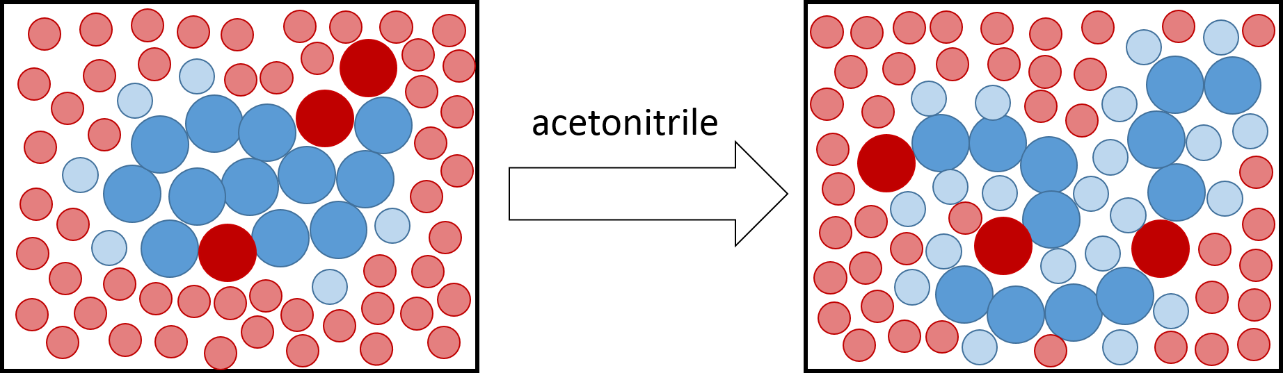
We simulate the behavior of the sequenced polysarcosine/poly (N-(2-carboxyethyl) glycine) diblock peptoid in a water-acetonitrile mixture for different acetonitrile concentrations. The sequenced polysarcosine/poly (N-(2-carboxyethyl) glycine) diblock peptoid chain includes 100 CG beads and the repeat unit is one (N-(2-carboxyethyl) glycine) bead and four sarcosine beads. In the experiment,⁶⁵ the polypeptoid chain were found to be coiled at low concentrations of acetonitrile and swell and form a globule at higher concentrations, as schematically shown in Figure 13. Our CG model predicts the $R_{g}$ in the coil state of $2.15\pm 0.19$nm, which is close to the $R_{g}$ values of 2.2 nm observed in the experiment⁶⁵. In the globule state, our model predicts $R_{g}=3.4\pm 0.25$nm, which is close the experimental value of $3.5$.

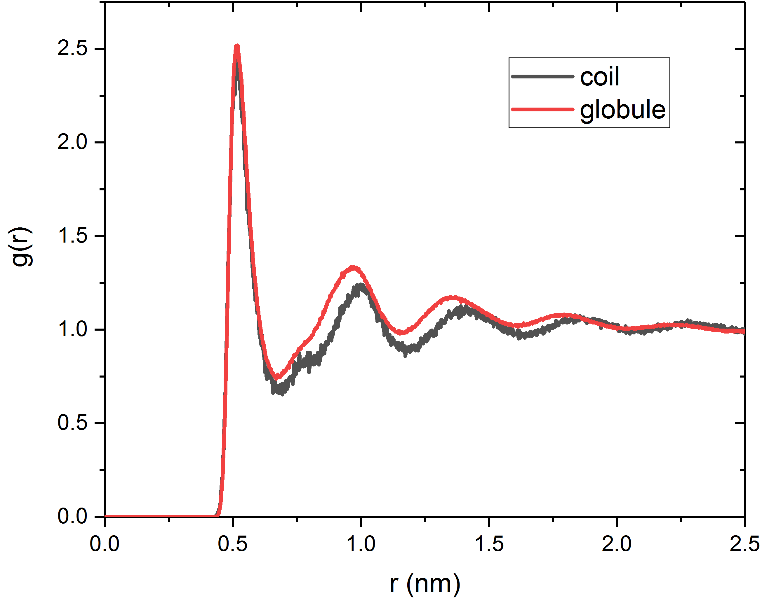
Figure 14 shows the peptoid RDF for the lowest and highest considered acetonitrile concentrations. The RDF peaks in the higher concentration mixture are higher than those in the lower concentration mixture. The increase in both RDF peaks and $R_{g}$ with the acetonitrile concentrations indicates that peptoids is swollen as the acetonitrile concentration increases.

4 Conclusion

In this paper, we proposed a new CG model for poly ($\alpha$-peptoid)s. We built the CG model for the poly ($\alpha$-peptoid) backbone (polysarcosine) in various solvents, including water, hexane, 1-octanol, and acetonitrile, and extended it to other peptoids. In our CG polypeptoid solution, we had three types of beads, including backbone, sidechain, and solvent beads, and the same degree of coarse-graining at in the MARTINI FF. This makes our model compatible with the MARTINI FF. All interactions between beads were divided into bonded interaction and nonbonded interaction. The bonded interactions between CG beads were parameterized to reproduce local and global structural properties including PDFs of bond length, bond angle, and dihedral angle and gyration radius obtained from atomic simulations of polypeptoids. Nonbonded potentials for water, hexane, and 1-octanol as well as potential for the interaction between hydrophilic or hydrophobic side chains and these solvents were taken from the MARTINI FF. The potential for acetonitrile and potentials between solvents and the backbone which are not given in MARTINI FF were parameterized by matching not only the transfer free energy but also the absolute solvation free energy. Our parameterization approach is expected to be more accurate than the approach in MARTINI FF where the target property is only the transfer free energy. The CG parameters of the backbone were extended to other peptoids with hydrophobic or hydrophilic side chains to examine transferability of the proposed CG model. We found that the hydration free energy of poly (N-(2-carboxyethyl) glycine) and poly (N-pentyl glycine) peptoids, computed from atomic simulations, is well reproduced by our CG model combining the proposed bonded potentials and nonbonded potentials with MARTINI FF. These results suggest that a CG model of any poly ($\alpha$-peptoid) can be constructed by adding side chains to our polysarcosine CG model with the nonbonded potentials given by MARTINI FF.

We evaluated the transferability of the bonded interaction parameters (bond, angle and torsion potentials) in the CG polysarcosine model by comparison of the local conformational PDFs of polysarcosine in various solvents. The previous CG models ^{68, 60} found that the bond and angle potentials to be transferable and torsion potential to be non-transferable in solution. In our CG model, the bond and angle potentials for polysarcosine are transferable for all considered solvents and the torsion potential is only transferable for good solvent. We demonstrated the transferability of torsion potential in good solvent with respect to the chain length by comparing the Rg of polysarcosine in a good solvent at modestly high molecular weight in atomic and CG simulations. We also found good transferability of the CG backbone parameter to poly (N-(2-carboxyethyl) glycine) in good solvent with respect to the chain length. Next, we demonstrated that the nonbonded potentials are transferable with respect to the solvation free energy for peptoids oligomers with the backbone made of five or less repeat units. We calculated the solvation free energy of two different polypeptoids, polysarcosine in acetonitrile and poly (N-(2-carboxyethyl) glycine) in water. The difference between the free energy in CG and atomic predictions for polysarcosine in acetonitrile is less than 6% for all considered chain lengths. The error in the solvation free energy of poly (N-(2-carboxyethyl) glycine) in water is less than 6% for chain length less than four repeat units and increases to about 16% for the five-unit-long peptoid chain. Note that the hydrogen bonding between side chains makes water like a poor solvent for poly (N-(2-carboxyethyl) glycine) in the atomic simulation here. Given that the torsion potential is not used for poly ($\alpha$-peptoid) backbone length less than four CG beads, the relatively large error for the peptoid with backbone larger than four beads indicate that the torsion potential has weak transferable in poor solvents. On the other hand, the simulations of polysarcosine in acetonitrile confirmed that the torsion potential is transferable in good solvents. Finally, we demonstrated that our CG model can describe the coil-to-globule transition of diblock polypeptoid chain in water-acetonitrile mixture and accurately predict the radius of gyration at both coil and globule states.

In this work, we demonstrated transferability of the CG potentials with respect to solvation free energy and conformation state. However, transferability of CG polymer model in solution with respect to other thermodynamic conditions remains an open question. For example, most of existing CG FF, including MARTINI FF, cannot describe phase transition (e.g., crystallization⁶⁹) of biopolymer because of the fixed backbone structure and complex interactions of the side chains. More advanced methods (e.g., machine learning) may be needed to generate adaptive CG potentials to describe the phase transition of polypeptoid solutions.

This work was supported by the U.S. Department of Energy (DOE), Office of Science, Office of Advanced Scientific Computing Research. Pacific Northwest National Laboratory is operated by Battelle for DOE under Contract DE-AC05-76RL01830.

The Supporting Information is available free of charge on the ACS Publications website.

References

- Robertson et al. 2016 Robertson, E. J.; Battigelli, A.; Proulx, C.; Mannige, R. V.; Haxton, T. K.; Yun, L.; Whitelam, S.; Zuckermann, R. N. Design, Synthesis, Assembly, and Engineering of Peptoid Nanosheets. Acc. Chem. Res. 2016, 49, 379–389
- Knight et al. 2017 Knight, A. S.; Kulkarni, R. U.; Zhou, E. Y.; Franke, J. M.; Miller, E. W.; Francis, M. B. A modular platform to develop peptoid-based selective fluorescent metal sensors. Chem. Commun. 2017, 53, 3477–3480
- Lau 2014 Lau, K. H. A. Peptoids for biomaterials science. Biomater. Sci. 2014, 2, 627–633
- Jun et al. 2015 Jun, J. M. V.; Altoe, M. V. P.; Aloni, S.; Zuckermann, R. N. Peptoid nanosheets as soluble, two-dimensional templates for calcium carbonate mineralization. Chem. Commun. 2015, 51, 10218–10221
- Merrill et al. 2018 Merrill, N. A.; Yan, F.; Jin, H.; Mu, P.; Chen, C.-L.; Knecht, M. R. Tunable assembly of biomimetic peptoids as templates to control nanostructure catalytic activity. Nanoscale 2018, 10, 12445–12452
- Patterson et al. 2017 Patterson, A. L.; Wenning, B.; Rizis, G.; Calabrese, D. R.; Finlay, J. A.; Franco, S. C.; Zuckermann, R. N.; Clare, A. S.; Kramer, E. J.; Ober, C. K. et al. Role of Backbone Chemistry and Monomer Sequence in Amphiphilic Oligopeptide- and Oligopeptoid-Functionalized PDMS- and PEO-Based Block Copolymers for Marine Antifouling and Fouling Release Coatings. Macromolecules 2017, 50, 2656–2667
- Reyes et al. 2014 Reyes, F. T.; Guo, L.; Hedgepeth, J. W.; Zhang, D.; Kelland, M. A. First Investigation of the Kinetic Hydrate Inhibitor Performance of Poly(N-alkylglycine)s. Energy and Fuels 2014, 28, 6889–6896
- Knight et al. 2015 Knight, A. S.; Zhou, E. Y.; Francis, M. B.; Zuckermann, R. N. Sequence Programmable Peptoid Polymers for Diverse Materials Applications. Adv. Mater. 2015, 27, 5665–5691
- Weber et al. 2018 Weber, B.; Birke, A.; Fischer, K.; Schmidt, M.; Barz, M. Solution Properties of Polysarcosine: From Absolute and Relative Molar Mass Determinations to Complement Activation. Macromolecules 2018, 51, 2653–2661
- Hara et al. 2014 Hara, E.; Ueda, M.; Makino, A.; Hara, I.; Ozeki, E.; Kimura, S. Factors Influencing in Vivo Disposition of Polymeric Micelles on Multiple Administrations. ACS Med. Chem. Lett. 2014, 5, 873–877
- Ueda et al. 2011 Ueda, M.; Makino, A.; Imai, T.; Sugiyama, J.; Kimura, S. Temperature-Triggered Fusion of Vesicles Composed of Right-Handed and Left-Handed Amphiphilic Helical Peptides. Langmuir 2011, 27, 4300–4304
- Sano et al. 2017 Sano, K.; Ohashi, M.; Kanazaki, K.; Makino, A.; Ding, N.; Deguchi, J.; Kanada, Y.; Ono, M.; Saji, H. Indocyanine Green-Labeled Polysarcosine for in Vivo Photoacoustic Tumor Imaging. Bioconjug. Chem. 2017, 28, 1024–1030
- Zhu et al. 2017 Zhu, H.; Chen, Y.; Yan, F.-J.; Chen, J.; Tao, X.-F.; Ling, J.; Yang, B.; He, Q.-J.; Mao, Z.-W. Polysarcosine brush stabilized gold nanorods for in vivo near-infrared photothermal tumor therapy. Acta Biomater. 2017, 50, 534–545
- Luxenhofer et al. 2013 Luxenhofer, R.; Fetsch, C.; Grossmann, A. Polypeptoids: A perfect match for molecular definition and macromolecular engineering? J. Polym. Sci., Part A: Polym. Chem. 2013, 51, 2731–2752
- Douy and Gallot 1987 Douy, A.; Gallot, B. Amphipathic block copolymers with two polypeptide blocks: Synthesis and structural study of poly(N-trifluoroacetyl-l-lysine)-polysarcosine copolymers. Polymer 1987, 28, 147–154
- Kimura and Imanishi 1983 Kimura, S.; Imanishi, Y. Synthesis and conformation of the cyclic octapeptides cyclo(Phe-Pro)4, cyclo(Leu-Pro)4, and cyclo[Lys(Z)-Pro]4. Biopolymers 1983, 22, 2191–2206
- Fokina et al. 2016 Fokina, A.; Klinker, K.; Braun, L.; Jeong, B. G.; Bae, W. K.; Barz, M.; Zentel, R. Multidentate Polysarcosine-Based Ligands for Water-Soluble Quantum Dots. Macromolecules 2016, 49, 3663–3671
- Klinker and Barz 2015 Klinker, K.; Barz, M. Polypept(o)ides: Hybrid Systems Based on Polypeptides and Polypeptoids. Macromol. Rapid Commun. 2015, 36, 1943–1957
- Hortz et al. 2015 Hortz, C.; Birke, A.; Kaps, L.; Decker, S.; Wächtersbach, E.; Fischer, K.; Schuppan, D.; Barz, M.; Schmidt, M. Cylindrical Brush Polymers with Polysarcosine Side Chains: A Novel Biocompatible Carrier for Biomedical Applications. Macromolecules 2015, 48, 2074–2086
- Birke et al. 2014 Birke, A.; Huesmann, D.; Kelsch, A.; Weilbächer, M.; Xie, J.; Bros, M.; Bopp, T.; Becker, C.; Landfester, K.; Barz, M. Polypeptoid-block-polypeptide Copolymers: Synthesis, Characterization, and Application of Amphiphilic Block Copolypept(o)ides in Drug Formulations and Miniemulsion Techniques. Biomacromolecules 2014, 15, 548–557
- Park and Szleifer 2011 Park, S. H.; Szleifer, I. Structural and Dynamical Characteristics of Peptoid Oligomers with Achiral Aliphatic Side Chains Studied by Molecular Dynamics Simulation. J. Phys. Chem. B 2011, 115, 10967–10975
- Mannige et al. 2015 Mannige, R. V.; Haxton, T. K.; Proulx, C.; Robertson, E. J.; Battigelli, A.; Butterfoss, G. L.; Zuckermann, R. N.; Whitelam, S. Peptoid nanosheets exhibit a new secondary-structure motif. Nature 2015, 526, 415–420
- Daily et al. 2016 Daily, M. D.; Baer, M. D.; Mundy, C. J. Divalent Ion Parameterization Strongly Affects Conformation and Interactions of an Anionic Biomimetic Polymer. J. Phys. Chem. B 2016, 120, 2198–2208
- Darré et al. 2015 Darré, L.; Machado, M. R.; Brandner, A. F.; González, H. C.; Ferreira, S.; Pantano, S. SIRAH: A Structurally Unbiased Coarse-Grained Force Field for Proteins with Aqueous Solvation and Long-Range Electrostatics. J. Chem. Theory Comput. 2015, 11, 723–739
- Mukherji et al. 2014 Mukherji, D.; Marques, C. M.; Kremer, K. Polymer collapse in miscible good solvents is a generic phenomenon driven by preferential adsorption. Nat. Commun. 2014, 5, 4882
- Agrawal et al. 2014 Agrawal, A.; Aryal, D.; Perahia, D.; Ge, T.; Grest, G. S. Coarse-Graining Atactic Polystyrene and Its Analogues. Macromolecules 2014, 47, 3210–3218
- Mantha and Yethiraj 2015 Mantha, S.; Yethiraj, A. Conformational Properties of Sodium Polystyrenesulfonate in Water: Insights from a Coarse-Grained Model with Explicit Solvent. J. Phys. Chem. B 2015, 119, 11010–11018
- Ozgur and Sayar 2016 Ozgur, B.; Sayar, M. Assembly of Triblock Amphiphilic Peptides into One-Dimensional Aggregates and Network Formation. J. Phys. Chem. B 2016, 120, 10243–10257
- de Oliveira et al. 2016 de Oliveira, T. E.; Netz, P. A.; Kremer, K.; Junghans, C.; Mukherji, D. C-IBI: Targeting cumulative coordination within an iterative protocol to derive coarse-grained models of (multi-component) complex fluids. J. Chem. Phys. 2016, 144, 174106
- Zhang and Guo 2014 Zhang, J.; Guo, H. Transferability of Coarse-Grained Force Field for nCB Liquid Crystal Systems. J. Phys. Chem. B 2014, 118, 4647–4660
- Gao and Guo 2015 Gao, P.; Guo, H. Developing coarse-grained potentials for the prediction of multi-properties of trans-1,4-polybutadiene melt. Polymer 2015, 69, 25–38
- Sauter and Grafmüller 2017 Sauter, J.; Grafmüller, A. Procedure for Transferable Coarse-Grained Models of Aqueous Polysaccharides. J. Chem. Theory Comput. 2017, 13, 223–236
- Abbott and Stevens 2015 Abbott, L. J.; Stevens, M. J. A temperature-dependent coarse-grained model for the thermoresponsive polymer poly(N-isopropylacrylamide). J. Chem. Phys. 2015, 143
- Kmiecik et al. 2016 Kmiecik, S.; Gront, D.; Kolinski, M.; Wieteska, L.; Dawid, A. E.; Kolinski, A. Coarse-Grained Protein Models and Their Applications. Chem. Rev. 2016,
- Poma et al. 2017 Poma, A. B.; Cieplak, M.; Theodorakis, P. E. Combining the MARTINI and Structure-Based Coarse-Grained Approaches for the Molecular Dynamics Studies of Conformational Transitions in Proteins. J. Chem. Theory Comput. 2017, 13, 1366–1374
- Cheon et al. 2010 Cheon, M.; Chang, I.; Hall, C. K. Extending the PRIME model for protein aggregation to all 20 amino acids. Proteins: Struct., Funct., Bioinf. 2010, 78, 2950–2960
- Gopal Srinivasa et al. 2009 Gopal Srinivasa, M.; Mukherjee, S.; Cheng, Y.; Feig, M. PRIMO/PRIMONA: A coarse‐grained model for proteins and nucleic acids that preserves near‐atomistic accuracy. Proteins: Struct., Funct., Bioinf. 2009, 78, 1266–1281
- Bereau and Deserno 2009 Bereau, T.; Deserno, M. Generic coarse-grained model for protein folding and aggregation. J. Chem. Phys. 2009, 130, 235106
- Haxton et al. 2015 Haxton, T. K.; Mannige, R. V.; Zuckermann, R. N.; Whitelam, S. Modeling Sequence-Specific Polymers Using Anisotropic Coarse-Grained Sites Allows Quantitative Comparison with Experiment. J. Chem. Theory Comput. 2015, 11, 303–315
- Marrink et al. 2007 Marrink, S. J.; Risselada, H. J.; Yefimov, S.; Tieleman, D. P.; de Vries, A. H. The MARTINI Force Field: Coarse Grained Model for Biomolecular Simulations. J. Phys. Chem. B 2007, 111, 7812–7824
- Cornell et al. 1995 Cornell, W. D.; Cieplak, P.; Bayly, C. I.; Gould, I. R.; Merz, K. M.; Ferguson, D. M.; Spellmeyer, D. C.; Fox, T.; Caldwell, J. W.; Kollman, P. A. A Second Generation Force Field for the Simulation of Proteins, Nucleic Acids, and Organic Molecules. J. Am. Chem. Soc. 1995, 117, 5179–5197
- Jorgensen et al. 1996 Jorgensen, W. L.; Maxwell, D. S.; Tirado-Rives, J. Development and Testing of the OPLS All-Atom Force Field on Conformational Energetics and Properties of Organic Liquids. J. Am. Chem. Soc. 1996, 118, 11225–11236
- Prakash et al. 2018 Prakash, A.; Baer, M. D.; Mundy, C. J.; Pfaendtner, J. Peptoid Backbone Flexibilility Dictates Its Interaction with Water and Surfaces: A Molecular Dynamics Investigation. Biomacromolecules 2018, 19, 1006–1015
- Wolfgang et al. 2011 Wolfgang, B.; Thomas, H.; Ludger, W. Systematic conformational investigations of peptoids and peptoid–peptide chimeras. J. Pept. Sci. 2011, 96, 651–668
- Mirijanian et al. 2014 Mirijanian, D. T.; Mannige, R. V.; Zuckermann, R. N.; Whitelam, S. Development and use of an atomistic CHARMM-based forcefield for peptoid simulation. J Comput. Chem. 2014, 35, 360–70
- MacKerell et al. 1998 MacKerell, A. D.; Bashford, D.; Bellott, M.; Dunbrack, R. L.; Evanseck, J. D.; Field, M. J.; Fischer, S.; Gao, J.; Guo, H.; Ha, S. et al. All-Atom Empirical Potential for Molecular Modeling and Dynamics Studies of Proteins. J. Phys. Chem. B 1998, 102, 3586–3616
- Jorgensen et al. 1983 Jorgensen, W. L.; Chandrasekhar, J.; Madura, J. D.; Impey, R. W.; Klein, M. L. Comparison of simple potential functions for simulating liquid water. J. Chem. Phys. 1983, 79, 926–935
- Hess et al. 1997 Hess, B.; Bekker, H.; Berendsen, H. J. C.; Fraaije, J. G. E. M. LINCS: A linear constraint solver for molecular simulations. J. Comput. Chem. 1997, 18, 1463–1472
- Essmann et al. 1995 Essmann, U.; Perera, L.; Berkowitz, M. L.; Darden, T.; Lee, H.; Pedersen, L. G. A smooth particle mesh Ewald method. J. Chem. Phys. 1995, 103, 8577–8593
- Bussi et al. 2007 Bussi, G.; Donadio, D.; Parrinello, M. Canonical sampling through velocity rescaling. J. Chem. Phys. 2007, 126, 014101
- Berendsen et al. 1984 Berendsen, H. J. C.; Postma, J. P. M.; van Gunsteren, W. F.; DiNola, A.; Haak, J. R. Molecular dynamics with coupling to an external bath. J. Chem. Phys. 1984, 81, 3684–3690
- Evans and Holian 1985 Evans, D. J.; Holian, B. L. The Nose–Hoover thermostat. J. Chem. Phys. 1985, 83, 4069–4074
- Parrinello and Rahman 1980 Parrinello, M.; Rahman, A. Crystal Structure and Pair Potentials: A Molecular-Dynamics Study. Phys. Rev. Lett. 1980, 45, 1196–1199
- Abraham et al. 2015 Abraham, M. J.; Murtola, T.; Schulz, R.; Páll, S.; Smith, J. C.; Hess, B.; Lindahl, E. GROMACS: High performance molecular simulations through multi-level parallelism from laptops to supercomputers. SoftwareX 2015, 1-2, 19–25
- Humphrey et al. 1996 Humphrey, W.; Dalke, A.; Schulten, K. VMD: Visual molecular dynamics. J. Mol. Graph. 1996, 14, 33–38
- Bennett 1976 Bennett, C. H. Efficient estimation of free energy differences from Monte Carlo data. J. Comput. Phys. 1976, 22, 245 – 268
- Kumar et al. 1992 Kumar, S.; Rosenberg, J. M.; Bouzida, D.; Swendsen, R. H.; Kollman, P. A. THE weighted histogram analysis method for free-energy calculations on biomolecules. I. The method. J. Comput. Chem. 1992, 13, 1011–1021
- Jorge et al. 2010 Jorge, M.; Garrido, N. M.; Queimada, A. J.; Economou, I. G.; Macedo, E. A. Effect of the Integration Method on the Accuracy and Computational Efficiency of Free Energy Calculations Using Thermodynamic Integration. J. Chem. Theory Comput. 2010, 6, 1018–1027
- Taddese and Carbone 2017 Taddese, T.; Carbone, P. Effect of Chain Length on the Partition Properties of Poly(ethylene oxide): Comparison between MARTINI Coarse-Grained and Atomistic Models. J. Phys. Chem. B 2017, 121, 1601–1609
- Dalgicdir et al. 2013 Dalgicdir, C.; Sensoy, O.; Peter, C.; Sayar, M. A transferable coarse-grained model for diphenylalanine: how to represent an environment driven conformational transition. J. Chem. Phys. 2013, 139, 234115
- Ryckaert and Bellemans 1978 Ryckaert, J.-P.; Bellemans, A. Molecular dynamics of liquid alkanes. Faraday Discuss. Chem. Soc. 1978, 66, 95–106
- Uttarwar et al. 2013 Uttarwar, R. G.; Potoff, J.; Huang, Y. Study on Interfacial Interaction between Polymer and Nanoparticle in a Nanocoating Matrix: A MARTINI Coarse-Graining Method. Ind. Eng. Chem. Res. 2013, 52, 73–82
- Bordner et al. 2002 Bordner, A. J.; Cavasotto, C. N.; Abagyan, R. A. Accurate Transferable Model for Water, n-Octanol, and n-Hexadecane Solvation Free Energies. J. Phys. Chem. B 2002, 106, 11009–11015
- Monticelli et al. 2008 Monticelli, L.; Kandasamy, S. K.; Periole, X.; Larson, R. G.; Tieleman, D. P.; Marrink, S. J. The MARTINI coarse-grained force field: Extension to proteins. J. Chem. Theory Comput. 2008, 4, 819–834
- Murnen et al. 2012 Murnen, H. K.; Khokhlov, A. R.; Khalatur, P. G.; Segalman, R. A.; Zuckermann, R. N. Impact of Hydrophobic Sequence Patterning on the Coil-to-Globule Transition of Protein-like Polymers. Macromolecules 2012, 45, 5229–5236
- Rubinstein and Colby 2003 Rubinstein, M.; Colby, R. H. Polymer Physics; Oxford University Press, 2003
- Tukhvatullin et al. 1999 Tukhvatullin, F. K.; Tashkenbaev, U. N.; Zhumaboev, A.; Mamatov, Z. Intermolecular hydrogen bonds in acetic acid and its solutions. J. Appl. Spectrosc. 1999, 66, 501–505
- Dalgicdir et al. 2016 Dalgicdir, C.; Globisch, C.; Sayar, M.; Peter, C. Representing environment-induced helix-coil transitions in a coarse grained peptide model. Eur. Phys. J. Spec. Top. 2016, 225, 1463–1481
- Shi et al. 2018 Shi, Z.; Wei, Y.; Zhu, C.; Sun, J.; Li, Z. Crystallization-Driven Two-Dimensional Nanosheet from Hierarchical Self-Assembly of Polypeptoid-Based Diblock Copolymers. Macromolecules 2018, 51, 6344–6351